chapter 4. electric stresses on cable insulation under standard and...
TRANSCRIPT
Chapter 4. Electric Stresses on Cable Insulation under Standard and Non-Standard Impulse Voltages
- 52 -
Chapter 4
Electric Stresses on Cable Insulation under Standard and Non-
standard Impulse Voltages
4.1 Cable Design
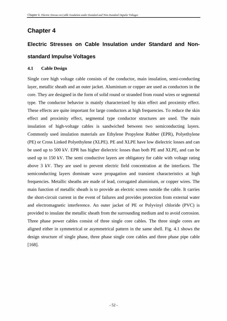
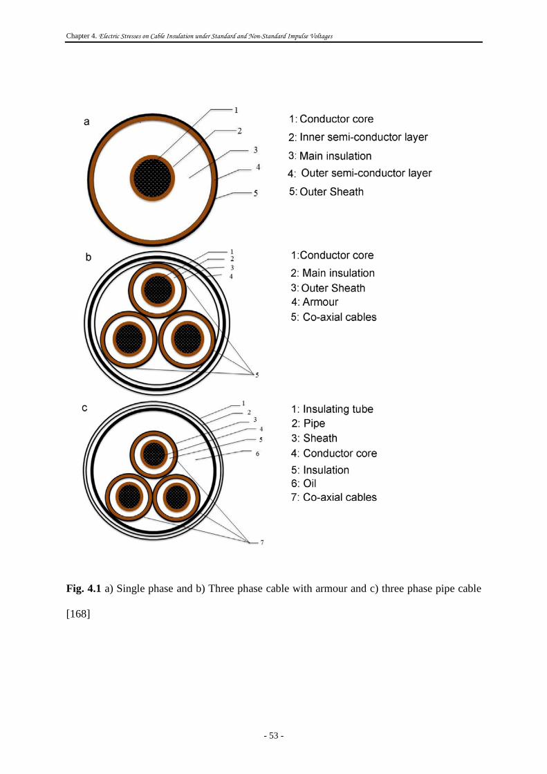
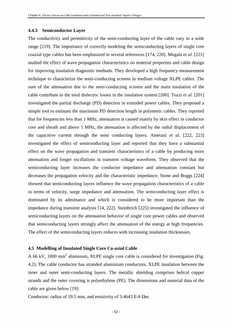
Single core high voltage cable consists of the conductor, main insulation, semi-conducting
layer, metallic sheath and an outer jacket. Aluminium or copper are used as conductors in the
core. They are designed in the form of solid round or stranded from round wires or segmental
type. The conductor behavior is mainly characterized by skin effect and proximity effect.
These effects are quite important for large conductors at high frequencies. To reduce the skin
effect and proximity effect, segmental type conductor structures are used. The main
insulation of high-voltage cables is sandwiched between two semiconducting layers.
Commonly used insulation materials are Ethylene Propylene Rubber (EPR), Polyethylene
(PE) or Cross Linked Polyethylene (XLPE). PE and XLPE have low dielectric losses and can
be used up to 500 kV. EPR has higher dielectric losses than both PE and XLPE, and can be
used up to 150 kV. The semi conductive layers are obligatory for cable with voltage rating
above 3 kV. They are used to prevent electric field concentration at the interfaces. The
semiconducting layers dominate wave propagation and transient characteristics at high
frequencies. Metallic sheaths are made of lead, corrugated aluminium, or copper wires. The
main function of metallic sheath is to provide an electric screen outside the cable. It carries
the short-circuit current in the event of failures and provides protection from external water
and electromagnetic interference. An outer jacket of PE or Polyvinyl chloride (PVC) is
provided to insulate the metallic sheath from the surrounding medium and to avoid corrosion.
Three phase power cables consist of three single core cables. The three single cores are
aligned either in symmetrical or asymmetrical pattern in the same shell. Fig. 4.1 shows the
design structure of single phase, three phase single core cables and three phase pipe cable
[168].
Chapter 4. Electric Stresses on Cable Insulation under Standard and Non-Standard Impulse Voltages
- 53 -
4.1 Investigation Approach
Fig. 4.1 a) Single phase and b) Three phase cable with armour and c) three phase pipe cable
[168]
Chapter 4. Electric Stresses on Cable Insulation under Standard and Non-Standard Impulse Voltages
- 54 -
4.2 Investigation Approach
A cable model developed in MATLAB©-Simulink based on design data of a 66 kV single
core cable system are used for transient analysis. The maximum permissible sheath armour
voltage for this cable is 33 kV and rated lightning withstand voltage is 325 kVp [169]. Four
different types of impulses were applied to the cable model at 325 kVp namely the standard
lightning impulse (1.2/50 µs), chopped impulse (3 µs), chopped impulse (15 µs) and non-
standard single pulse and damped oscillating impulse waveform. The non-standard impulse
waveforms are used in order to denote some more realistic waveforms than the typical
standard waveform. Important standards used for cable impulse testing are IEEE Std. 82-
2002 [80], IEEE Std. 1243 [170], IEC 60141-1 [109], IEC 60840 [111], IEC 60229 [113],
IEC 62067 [118]. To investigate the overvoltage stress in the cable against impulse
waveforms, the maximum sheath potential to ground for 1 m, 7 m, 14 m, 21 m, 28 m and 35
m of cable is observed.
4.3 Cable Modelling Approaches
The underground cable models are generally based on transmission line theory [14].
Transient response analysis requires accurate mathematical representation of power cable
parameters over a wide range of frequencies. The analysis of various electromagnetic
phenomena that take place in the conductor, semi-conductor and insulation of the cable,
distributed nature of transmission line parameters, asymmetrical arrangement of coupled
conductors with ground return etc. are required to be considered to achieve better accuracy in
modeling [15]. The commonly used approaches for insulated cable modeling are lumped
parameter and the distributed travelling wave models. A lumped model of overhead
transmission line or cable consists of arrangement of R, L, and C parameters in the form of pi
(π). The shunt losses associated with the model and voltages at the cross bonding of sheaths
are ignored. This model is suitable only for steady state analysis with limited range of
frequencies. Nagaoka and Ametani [16] proposed a cross bonded uniform pi cable model. In
this model, the sheath voltage at the cross bonding points could be measured at major
sections of the cable length. This makes it inadequate for predicting frequency response for a
wide range of frequency. Budner [17] developed an exact pi-model which could predict well
the frequency response but it requires high computation time [18]. The distributed parameter
travelling wave model includes the frequency dependent approach and is therefore preferred
over the lumped parameter model. J. R. Marti [19] proposed the frequency dependent
Chapter 4. Electric Stresses on Cable Insulation under Standard and Non-Standard Impulse Voltages
- 55 -
travelling wave models of overhead lines and cables which included line losses and
frequency dependence of line parameters. However, this model had limitations due to use of
real and constant transformation matrix between the actual phase and the modal domain
variables. Real and constant transformation matrices provide inaccurate results for un-
transposed or asymmetrically arranged conductors in poly-phase cables due to the frequency
dependence of internal resistances, inductances and ground return impedances. With this, the
need for frequency dependent line or cable parameters and modal transformation matrices
was felt. L. Marti [20] proposed a new model which carried out the transformation as a real
time convolution taking into account the frequency dependence of transmission matrix.
However, it requires determination of a suitable frequency for approximation of the modal
transformation matrices. It worked well in both low and high frequency ranges for
underground cables. Dommel [21] was the first to develop transmission line model in
EMTPTM based on distributed parameter model. The frequency response of this model was
found to be satisfactory in the vicinity of the frequency at which the parameters are evaluated.
Ali Abur et al. [22] used wavelet-transform based method for taking into account the
frequency dependence of modal transformation matrices. This method offered the advantage
of transient modeling and simulations using frequency dependent parameters in the time
domain. Another method of taking the frequency dependence of the transformation matrix
into account was proposed by Nakanishi et al. [23] and Mahmutcehajic et al. [24]. They
obtained transmission line parameters in the actual phase domain using frequency-transform
technique (Laplace transform and Hartley transform method respectively) and used the
method of the superposition law for calculating transmission line transients. Semlyen et al.
[25] developed a model in EMTPTM type suite. They obtained frequency dependent
parameters suitable for a wide range of frequencies using recursive calculations by expressing
step responses with exponential functions. Using recursive convolutions resulted in reduced
computational time [25]. Lee and Poon [26] used constant parameter representation to model
un-transposed transmission lines in EMTPTM. It had the limitation that the modal
transformation matrices have to be calculated manually. Moreover, the frequency dependent
nature of cables is not represented properly by this model. Gustavsen et al. [27] also
presented frequency dependent modeling using the recursive convolutions in phase domain.
They obtained recursive convolutions by fitting the tail portion of the time step responses
with piecewise linear functions. Further, to achieve computational efficiency, they proposed a
robust vector fitting technique for transformation matrix and the modal characteristic
admittance [28]. This fitting process used modal decomposition and frequency dependent

Chapter 4. Electric Stresses on Cable Insulation under Standard and Non-Standard Impulse Voltages
- 56 -
transformation matrices. Phase-domain computations are done based on Two Sided
Recursions (TSR) or short convolutions performed on both input and output variables [29].
Another phase domain approach using an ARMA (Auto-Regressive Moving Average) model
was presented by Noda et al.[30]. ARMA model has advantages of reduced computational
time, increased stability, linear optimizations etc. over the modal domain based models.
Another advantage is that the modeling is directly performed in the phase domain which
avoids the use of frequency dependent transformation matrices. A new development in
electromagnetic transient analysis of multi-conductor power transmission lines was the use of
Z-transform. The disadvantage associated with this approach is that Z-transform inhibits the
model’s application in arbitrary time step [31]. Humpage et al. [32] used Z-transform
formulation to obtain transient analysis solutions in time domain from the frequency domain.
Huang and Semlyen [33] developed a three phase transmission line model and emphasized
upon considering effects of corona along with frequency dependence of line parameters.
Castellanos and Marti [34] and Yu and Marti [35] followed the work of Huang and Semlyen
[33] but the frequency dependence of the modal transformation matrix was taken into account
by carrying out the calculations in the actual phase domain. This approach provided
numerically stable functions over a wide range of frequencies.
4.4 Parameter Sensitivity
4.4.1 Earth Return Impedances
In transient simulations, the cable parameters are strongly influenced by the resistive earth
return path impedances [171]. The modeling of earth return impedances is important to take
into account the resistive losses due to the imperfectly conducting ground and in the
calculations of lightning induced currents and voltages on buried cables above 1 MHz [14,
172-175]. Carson [176] was the first to investigate earth return impedance in overhead lines
and Pollaczek [177] investigated for both underground and the combinations of underground
and overhead conductors. Both of them assumed earth to be homogeneous and semi-infinite
and expressed the earth return impedance by infinite integral involving complex Bessel
functions [171]. Carson [176] and Pollaczek [177] did not consider the effect of displacement
current in calculations of earth return impedance formulas which are important for high
frequency studies [178]. Pollaczek’s [177] integral for the ground impedance is expressed as
equation (4.1). The accurate evaluation of the Bessel functions and infinite integrals is
obtained using approximate expressions or numerical integration algorithms [14].
Chapter 4. Electric Stresses on Cable Insulation under Standard and Non-Standard Impulse Voltages
- 57 -
Z′g = 𝑗𝑗ω2πµ0 [K0 (
𝑏𝑏𝑝𝑝) – K0 (
2𝑑𝑑𝑝𝑝
) + J] (4.1)
where
𝐽𝐽 = ∫exp[−2d𝛽𝛽2+ 1
𝑝𝑝2 ]
β+𝛽𝛽2+ 1𝑝𝑝2
exp(jωb) dβ∞−∞ (4.2)
j is the imaginary unit,
K0 is the modified Bessel function of second class and zero order,
p is the complex depth of skin effect layer, and
d is the depth of the cable.
Sunde [179] improved Pollaczek’s formulas for using it at higher frequencies by including
the displacement current and influence of earth permittivity on the earth return impedances of
a single buried cable. Wise [180] added earth admittance correction terms in Carson’s
formula to calculate accurately the propagation characteristics of overhead transmission lines
at higher frequencies. Vance [181] proposed a simplified expression for the ground
admittance of a single conductor cable using Hankel functions. Petrache et al. [175] pointed
out that ground admittance plays an important role for the buried cables at high frequencies
(1 MHz or so) and showed the analogy between Pollaczek’s [177] and Sunde’s [179] earth
return impedance calculation formulas. Further, they investigated applicability of Pollaczek
[177], Sunde [179], Vance [181], Semlyen and Wedepohl [182], Saad–Gaba–Giroux [183]
and Bridges [184] formula for the ground impedance and reported that within the frequency
range of 1 kHz–30 MHz all the considered expressions provided similar results. However,
they proposed a simple logarithmic approximation for the ground impedance as given by
equation (4.3)
𝑍𝑍𝑔𝑔𝑙𝑙𝑙𝑙𝑔𝑔 = 𝑗𝑗𝑗𝑗
2𝜋𝜋µ0 ln (1+ 𝛾𝛾𝑔𝑔 . 𝑏𝑏
𝛾𝛾𝑔𝑔 . 𝑏𝑏 ) (4.3)
where γg is the propagation constant in the ground, b is radius of the cable.
Chapter 4. Electric Stresses on Cable Insulation under Standard and Non-Standard Impulse Voltages
- 58 -
This logarithmic expression is similar to Sunde’s expression except that it is independent of
the burial depth. It’s implementation is very simple and does not require any numerical
treatment. Also, it shows an asymptotic behaviour at high frequencies [175].
Ametani et al. [185] investigated numerical instability issues in the mutual impedance
formula proposed by Pollaczek [177]. Their investigation reported that numerical instability
of the infinite integral is caused by incorrect integrand in high-frequency region. Wedepohl
and Wilcox [39] calculated the frequency dependent earth return impedances of buried
cables. The following expression (4) for the ground impedance was reported in [182]:
Z’g = 𝑗𝑗𝑗𝑗2𝜋𝜋µ0 ln (b + 1
𝑚𝑚𝑏𝑏) (4.4)
where m = √(𝑗𝑗ωµ0σg)
’m’ is the propagation constant of the ground, neglecting the displacement current, σg is the
ground conductivity, µ0 is the free space permeability.
Uribe and Ramirez [186] further extended the calculations of ground return impedances of
buried cables by numerical analysis combining Wedepohl and Wilcox series and the
trapezoidal rule of integration. Jun et al. [187] proposed an efficient and generalized
algorithm to calculate the earth return impedance using the moment technique. They
approximated the non oscillatory part of the integrand without the cosine function using
piecewise quadratic functions, and expressed the Pollaczek integral [177] in a closed form
with the help of the moment functions. Recently, Theodoulidis [188] presented three exact
solutions of pollaczek's integral using mathematical packages or available routines. The three
solutions are in the form of converging series expressed in terms of Bessel functions of half
an odd integer order or in terms of the confluent hypergeometric function. Papagiannis et al.
[171] proposed a direct numerical integration scheme for the evaluation of oscillating infinite
integral during the calculation of the earth return impedances for the case of homogeneous
earth. Their method did not use approximations and showed remarkable numerical stability
and efficiency. Legrand et al. [189] computed Pollaczek’s integral based on a quasi-Monte
Carlo method with Van Der Corput series. Their proposed method presented a fast
convergence rate, error bound, and most importantly, the computing time was independent of
the integral function. Expressions for the earth return impedance in power cables buried in a
two-layer earth was proposed by Tsiamitros et al. [190]. They ignored the influence of the
Chapter 4. Electric Stresses on Cable Insulation under Standard and Non-Standard Impulse Voltages
- 59 -
non-homogeneous earth on the shunt admittances and studied only the influence of two-layer
earth structure on the series impedances of underground power cables. Their formula is valid
for few kHz frequency range only. The influences of the imperfect earth on cable admittances
for fast transient simulations have been studied in detail by several researchers [191-195].
Theethayi et al. [192] investigated the applicability of some closed form expressions for the
ground impedance and ground admittance of buried bare and insulated horizontal wires based
on transmission line (TL) theory for a wide frequency range (up to 10 MHz). They used
Vance’s ground admittance formula to study the transient responses of underground cables.
Investigation results showed that the low frequency approximation of the ground impedance
for cases of high resistivity soils leads to inaccurate results [192, 196]. They observed that the
ground impedance is more sensitive whereas the ground admittance is less sensitive to
ground conductivity. Ametani [178] formulated the impedances and admittances of single-
core coaxial cables and pipe-type cables. He also developed EMTP support routines for the
calculation of the series and shunt impedances of single core coaxial cables and high voltage
pipe type cables. Ferkal et al. [197] proposed to calculate the current distribution in the core
and the layer of a single-core cable using Maxwell equations. Accurate earth models for the
homogeneous and the two-layer earth case have been proposed recently in [194, 196]
Papadopoulos et al. [196] obtained the expressions for the shunt admittances and the series
impedances of underground multi-conductor single-core power cables in arbitrary
arrangements. They used electromagnetic field theory assuming quasi-TEM-field propagation
for the calculations. This means that this approach can be valid up to the MHz frequency
range in conjunction with earth resistivity not exceeding 1000 Ω m. Papadopoulos et al. [194]
investigated the influence of a two-layer earth structure in the shunt admittances of an
underground power cable over a wide frequency range. They calculated the shunt
admittances of an underground power cable for various two-layer earth configurations by EM
field equations using the Hertzian vector approach and improved the series impedance
calculation formulas of previous contributions by including a propagation term. The resulting
expressions are used in transient calculations to include a more accurate model in the
simulation of underground cable transients [47].
4.4.2 Skin and Proximity Effect
The series impedance, Z is characterized by both skin and proximity effect [198]. Skin and
proximity effects cause non uniform current distributions in the conductors. Xu et al. [199]
investigated for the first time the mechanisms of high frequency loss in shielded power cables
Chapter 4. Electric Stresses on Cable Insulation under Standard and Non-Standard Impulse Voltages
- 60 -
and reported that skin effect losses in the conductor increases as the square root of frequency.
The main cause of attenuation in power cables at frequencies below 1 MHz is due to skin
effect losses in core and sheath [199-201]. The wave propagation characteristic on cables
considering the proximity effect was investigated by Kawamura et al. [202]. Investigation
results showed that proximity effect increases the attenuation and decreases the characteristic
impedance of the cable. The effect is more noticeable at very high frequencies (>100 MHz)
when cables are placed together [203]. Gustavsen et al. [198] calculated the sheath voltages
for three single core coaxial cable systems. They reported that the sheath voltages depend on
the proximity effect and the helical winding of the sheath wires. Finite element techniques
(FEM) have been used for calculating cable parameters taking into account skin and
proximity effects in several published works [204-208]. This technique allows analysis of
extremely complex geometric configurations and also diverse insulating materials with
different dielectric characteristics. Gustavsen et al. [209] introduced two dimensional (2-D)
finite element computations for the calculation of series impedance and the shunt capacitance
of umbilical cables. Three dimensional (3-D) finite element analysis of skin effect in current-
carrying conductors was used by Kim et al.[210]. Comellini et al. [211] and Paloma [212]
used the partial sub-conductors method to estimate skin and proximity effects of stranded and
sector shaped conductors based on subdivision of conductors. The main advantage of this
method over the finite element methods is that the earth return path does not need to be
subdivided. Lukas and Talukdar [204] applied the sub-conductors technique to the calculation
of the frequency dependent parameters of co axial cables. They divided the conductors into
arc shaped sub conductors and named them elementals. These elementals are implemented in
the inductance formulae to include necessary arbitrary shapes. Weiss and Csendes [213]
developed a one-step procedure to solve the skin effect problem in multi conductor bus bars.
They calculated impedances as part of the solution vector. Papagiannis [214] also used one-
step finite element formulation but for the modeling of single and double-circuit transmission
lines of arbitrary geometry. Rivas and Marti [215] presented a new algorithm using digital
images for the calculation of the frequency-dependent parameters of arbitrarily shaped power
cable arrangements. The algorithm discretized the cable geometry and partial sub conductor
equivalent circuit method to estimate the cable parameters. Pagnetti et al. [216] proposed a
semi-analytical method including proximity effect for the evaluation of internal impedances
of solid and hollow conductors. Bormann and Tavakoli [217] used reluctance network
method for calculating the series impedance matrix of multi-conductor transmission lines. An
equivalent surface current approach was proposed for inclusion of skin and proximity effects

Chapter 4. Electric Stresses on Cable Insulation under Standard and Non-Standard Impulse Voltages
- 61 -
by Patel et al. [218]. The method was based on a surface admittance operator in combination
with the method of moments.
Chapter 4. Electric Stresses on Cable Insulation under Standard and Non-Standard Impulse Voltages
- 62 -
4.4.3 Semiconductor Layer
The conductivity and permittivity of the semi-conducting layer of the cable vary in a wide
range [219]. The importance of correctly modeling the semiconducting layers of single core
coaxial type cables has been emphasized in several references [174, 220]. Mugala et al. [221]
studied the effect of wave propagation characteristics on material properties and cable design
for improving insulation diagnostic methods. They developed a high frequency measurement
technique to characterize the semi-conducting screens in medium voltage XLPE cables. The
sum of the attenuation due to the semi-conducting screens and the main insulation of the
cable contribute to the total dielectric losses in the insulation system [200]. Tozzi et al. [201]
investigated the partial discharge (PD) detection in extruded power cables. They proposed a
simple tool to estimate the maximum PD detection length in polymeric cables. They reported
that for frequencies less than 1 MHz, attenuation is caused mainly by skin effect in conductor
core and sheath and above 1 MHz, the attenuation is affected by the radial displacement of
the capacitive current through the semi conducting layers. Ametani et al. [222, 223]
investigated the effect of semiconducting layer and reported that they have a substantial
effect on the wave propagation and transient characteristics of a cable by producing more
attenuation and longer oscillations in transient voltage waveform. They observed that the
semiconducting layer increases the conductor impedance and attenuation constant but
decreases the propagation velocity and the characteristic impedance. Stone and Boggs [224]
showed that semiconducting layers influence the wave propagation characteristics of a cable
in terms of velocity, surge impedance and attenuation. The semiconducting layer effect is
dominated by its admittance and which is considered to be more important than the
impedance during transient analysis [14, 222]. Steinbrich [225] investigated the influence of
semiconducting layers on the attenuation behavior of single core power cables and observed
that semiconducting layers strongly affect the attenuation of the energy at high frequencies.
The effect of the semiconducting layers reduces with increasing insulation thicknesses.
4.5 Modelling of Insulated Single Core Co-axial Cable
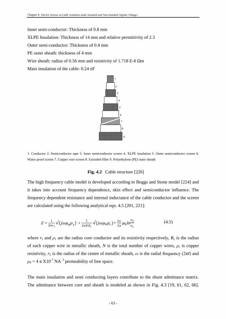
A 66 kV, 1000 mm2 aluminum, XLPE single core cable is considered for investigation (Fig.
4.2). The cable conductor has stranded aluminium conductors, XLPE insulation between the
inner and outer semi-conducting layers. The metallic shielding comprises helical copper
strands and the outer covering is polyethylene (PE). The dimensions and material data of the
cable are given below [19]:
Conductor: radius of 19.5 mm, and resistivity of 3.4643 E-8 Ωm
Chapter 4. Electric Stresses on Cable Insulation under Standard and Non-Standard Impulse Voltages
- 63 -
Inner semi-conductor: Thickness of 0.8 mm
XLPE Insulation: Thickness of 14 mm and relative permittivity of 2.3
Outer semi-conductor: Thickness of 0.4 mm
PE outer sheath: thickness of 4 mm
Wire sheath: radius of 0.56 mm and resistivity of 1.718 E-8 Ωm
Main insulation of the cable: 0.24 nF
1. Conductor 2. Semiconductor tape 3. Inner semiconductor screen 4. XLPE insulation 5. Outer semiconductor screen 6.
Water proof screen 7. Copper wire screen 8. Extruded filler 9. Polyethylene (PE) outer sheath
Fig. 4.2 Cable structure [226]
The high frequency cable model is developed according to Boggs and Stone model [224] and
it takes into account frequency dependence, skin effect and semiconductor influence. The
frequency dependent resistance and internal inductance of the cable conductor and the screen
are calculated using the following analytical eqn. 4.5 [201, 221]:
Z = 12𝜋𝜋𝑟𝑟1
√(𝑗𝑗𝑗𝑗𝜇𝜇0𝜌𝜌1) + 12𝜋𝜋𝜋𝜋𝑅𝑅𝑐𝑐
√(𝑗𝑗𝑗𝑗𝜇𝜇0𝜌𝜌𝑐𝑐)+ 𝑗𝑗𝑗𝑗2𝜋𝜋𝜇𝜇0ln
𝑟𝑟2𝑟𝑟1
where r1 and ρ1 are the radius core conductor and its resistivity respectively, Rc is the radius
of each copper wire in metallic sheath, N is the total number of copper wires, ρc is copper
resistivity, r2 is the radius of the centre of metallic sheath, ω is the radial frequency (2πf) and
μ0 = 4 π X10-7 NA−2 permeability of free space.
The main insulation and semi conducting layers contribute to the shunt admittance matrix.
The admittance between core and sheath is modeled as shown in Fig. 4.3 [19, 61, 62, 66].
(4.5)
Chapter 4. Electric Stresses on Cable Insulation under Standard and Non-Standard Impulse Voltages
- 64 -
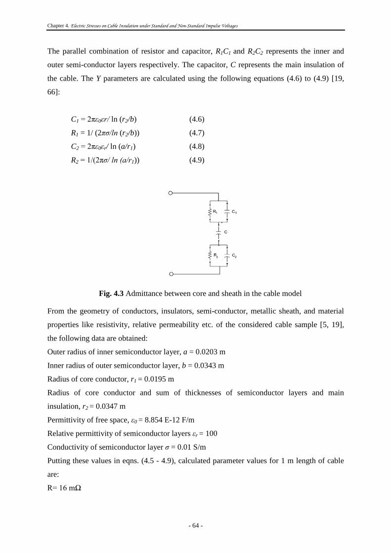
The parallel combination of resistor and capacitor, R1C1 and R2C2 represents the inner and
outer semi-conductor layers respectively. The capacitor, C represents the main insulation of
the cable. The Y parameters are calculated using the following equations (4.6) to (4.9) [19,
66]:
C1 = 2πε0εr/ ln (r2/b) (4.6)
R1 = 1/ (2πσ/ln (r2/b)) (4.7)
C2 = 2πε0εr/ ln (a/r1) (4.8)
R2 = 1/(2πσ/ ln (a/r1)) (4.9)
Fig. 4.3 Admittance between core and sheath in the cable model
From the geometry of conductors, insulators, semi-conductor, metallic sheath, and material
properties like resistivity, relative permeability etc. of the considered cable sample [5, 19],
the following data are obtained:
Outer radius of inner semiconductor layer, a = 0.0203 m
Inner radius of outer semiconductor layer, b = 0.0343 m
Radius of core conductor, r1 = 0.0195 m
Radius of core conductor and sum of thicknesses of semiconductor layers and main
insulation, r2 = 0.0347 m
Permittivity of free space, ε0 = 8.854 E-12 F/m
Relative permittivity of semiconductor layers εr = 100
Conductivity of semiconductor layer σ = 0.01 S/m
Putting these values in eqns. (4.5 - 4.9), calculated parameter values for 1 m length of cable
are:
R= 16 mΩ
Chapter 4. Electric Stresses on Cable Insulation under Standard and Non-Standard Impulse Voltages
- 65 -
L= 0.28 µH
C1= 0.479 µH
C2= 0.138 µH
C= 0.24 nF
R1= 1.848 Ω and
R2= 6.41 Ω.
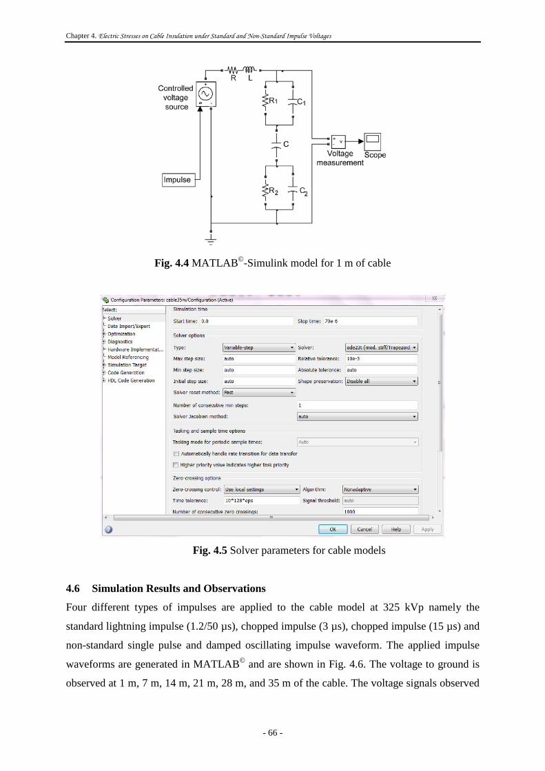
The per unit length (1 m) parameters used to represent electromagnetic field effects and
losses of the single core coaxial cable are deduced using the approaches presented in [5, 19,
61, 62, 66]. The per unit length (1 m) circuit of the cable model is shown in Fig. 4.4. The
developed cable model consists of the following blocks:
a. The controlled voltage source block converts the Simulink input signal into an equivalent
voltage source. The input signal to this block is an impulse voltage (standard and non-
standard impulse) generated in MATLAB©.
b. Series combination of resistor and inductor R and L, representing the core conductor of the
cable.
c. Parallel combination of resistor and capacitor, R1C1 and R2C2 representing the semi-
conductor screens.
d. Single capacitor, C representing the main insulation.
e. The voltage measurement block measures the instantaneous voltage between two nodes.
f. Scope displays the output signal. The displayed waveforms are then used to measure time
and voltage values.
Chapter 4. Electric Stresses on Cable Insulation under Standard and Non-Standard Impulse Voltages
- 66 -
Fig. 4.4 MATLAB©-Simulink model for 1 m of cable
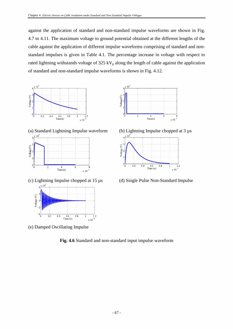
Fig. 4.5 Solver parameters for cable models
4.6 Simulation Results and Observations
Four different types of impulses are applied to the cable model at 325 kVp namely the
standard lightning impulse (1.2/50 µs), chopped impulse (3 µs), chopped impulse (15 µs) and
non-standard single pulse and damped oscillating impulse waveform. The applied impulse
waveforms are generated in MATLAB© and are shown in Fig. 4.6. The voltage to ground is
observed at 1 m, 7 m, 14 m, 21 m, 28 m, and 35 m of the cable. The voltage signals observed
Chapter 4. Electric Stresses on Cable Insulation under Standard and Non-Standard Impulse Voltages
- 67 -
against the application of standard and non-standard impulse waveforms are shown in Fig.
4.7 to 4.11. The maximum voltage to ground potential obtained at the different lengths of the
cable against the application of different impulse waveforms comprising of standard and non-
standard impulses is given in Table 4.1. The percentage increase in voltage with respect to
rated lightning withstands voltage of 325 kVp along the length of cable against the application
of standard and non-standard impulse waveforms is shown in Fig. 4.12.
(a) Standard Lightning Impulse waveform (b) Lightning Impulse chopped at 3 µs
(c) Lightning Impulse chopped at 15 µs (d) Single Pulse Non-Standard Impulse
(e) Damped Oscillating Impulse
Fig. 4.6 Standard and non-standard input impulse waveform

Chapter 4. Electric Stresses on Cable Insulation under Standard and Non-Standard Impulse Voltages
- 68 -
(a) Voltage to ground observed in 1 m (b) Voltage to ground observed in 7 m
(c) Voltage to ground observed in 14 m (d) Voltage to ground observed in 21 m
(e) Voltage to ground observed in 28 m (f) Voltage to ground observed in 35 m
Fig. 4.7 Voltage to ground observed in 1 m, 7 m, 14 m, 21 m, 28 m, and 35 m of the 66 kV
cable against the application of full lightning impulse.

Chapter 4. Electric Stresses on Cable Insulation under Standard and Non-Standard Impulse Voltages
- 69 -
(a) Voltage to ground observed in 1 m (b) Voltage to ground observed in 7 m
(c) Voltage to ground observed in 14m (d) Voltage to ground observed in 21m
(e) Voltage to ground observed in 28 m (f) Voltage to ground observed in 35 m
Fig. 4.8 Voltage to ground observed in 1 m, 7 m, 14 m, 21 m, 28 m, and 35 m of 66 kV cable
against the application of chopped (3 µs) impulse.
Chapter 4. Electric Stresses on Cable Insulation under Standard and Non-Standard Impulse Voltages
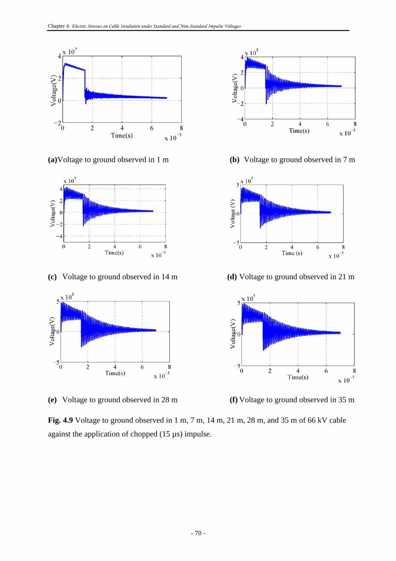
- 70 -
(a) Voltage to ground observed in 1 m (b) Voltage to ground observed in 7 m
(c) Voltage to ground observed in 14 m (d) Voltage to ground observed in 21 m
(e) Voltage to ground observed in 28 m (f) Voltage to ground observed in 35 m
Fig. 4.9 Voltage to ground observed in 1 m, 7 m, 14 m, 21 m, 28 m, and 35 m of 66 kV cable
against the application of chopped (15 µs) impulse.

Chapter 4. Electric Stresses on Cable Insulation under Standard and Non-Standard Impulse Voltages
- 71 -
(a) Voltage to ground observed in 1 m (b) Voltage to ground observed in 7 m
(c) Voltage to ground observed in 14 m (d) Voltage to ground observed in 21 m
(e) Voltage to ground observed in 28 m (f) Voltage to ground observed in 35 m
Fig. 4.10 Voltage to ground observed in 1 m, 7 m, 14 m, 21 m, 28 m, and 35 m of 66 kV
cable against the application of single pulsed impulse.
Chapter 4. Electric Stresses on Cable Insulation under Standard and Non-Standard Impulse Voltages
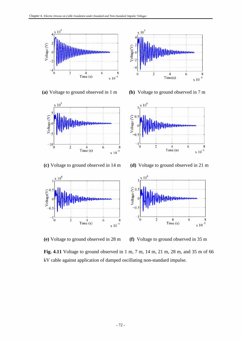
- 72 -
(a) Voltage to ground observed in 1 m (b) Voltage to ground observed in 7 m
(c) Voltage to ground observed in 14 m (d) Voltage to ground observed in 21 m
(e) Voltage to ground observed in 28 m (f) Voltage to ground observed in 35 m
Fig. 4.11 Voltage to ground observed in 1 m, 7 m, 14 m, 21 m, 28 m, and 35 m of 66
kV cable against application of damped oscillating non-standard impulse.

Chapter 4. Electric Stresses on Cable Insulation under Standard and Non-Standard Impulse Voltages
- 73 -
Table 4.1 Maximum voltage obtained against the application of standard and non-standard
impulse waveforms
Applied Impulses Maximum voltage to ground (kV) observed at cable length (s) 1 m 7 m 14 m 21 m 28 m 35 m
Full standard lightning 334.5 377.5 421 455.6 481.2 488.4
Impulse chopped at 3 µs 334.8 377.9 423 456 481 490 Impulse chopped at 15 µs 334.5 378 420 456 480 488.2 Non-standard single pulsed 335 405 475 527 562 574
Non-standard Damped oscillating 334.5 377.7 420 456 481 490
(a)
(b)
Fig. 4.12 Variation of voltage increase along the cable against the application of different
impulse waveforms.

Chapter 4. Electric Stresses on Cable Insulation under Standard and Non-Standard Impulse Voltages
- 74 -
4.7 Conclusions
In this chapter, a 66 kV underground single core cable has been used to study the effect of
standard and non-standard lightning impulse waveforms. Transient response is studied
against the variation of four different types of impulse voltage waveshapes comprising of
standard full waveform, chopped and non-standard, oscillating and non-oscillating impulses
along different lengths of the cable. A preliminary comparative study on the obtained
voltages indicated that non-standard single pulse impulse waveform developed higher voltage
stress in the cable. The results provide the basis for detailed experimental test and thereby
make necessary correction in the standards. The main observations are summarized below:
I. For the same applied transient peak voltage, the voltage crest across the cable keeps on
increasing with increasing cable length.
II. The general trends of voltage increase except that of the 1 m length is same for all cable
lengths. It is thus evident that cable length and impinging voltage shapes strongly
influence the overvoltage attenuation in the cable.
III. The maximum voltage profile is obtained for the non-standard single pulsed waveform
compared to the standard full lightning impulse waveform for 35 m length of the cable
(increase by 17.53%).