chapter 4 materials and methods -...

36

CHAPTER 4

MATERIALS AND METHODS

4.1 GENERAL

Our earth has almost three-fourth of its surface covered by water.

Water pumped is being used for various purposes. For the past twenty years,

many industries and factories are set up due to the dynamic growth of

globalization and strong financial support of the government. When water

gets mingled with the garbage and effluents through industries, it loses its

originality. Water which gets contaminated due to the threat of environments

is cause for spread of epidemic diseases. The polluted water affects health of

all beings. It is felt that water analysis has to be carried out for critical water

quality parameters.

Regarding the water quality monitoring, scientists and technical

experts do their research. Investigations go on to identify the polluted areas.

Therefore, necessity of monitoring on the water quality has arisen. This

chapter deals with materials used and methods adopted to probe quality of

water. Water springs from natural sources and so it is duty of everyone to

keep water from deterioration. The study area gives a clear picture about

impure water quality which is available on account of effluents treated by

traditional sectors of industry such as textiles, chemical industries and

engineering goods. To be free from hazardous health, water quality is to be

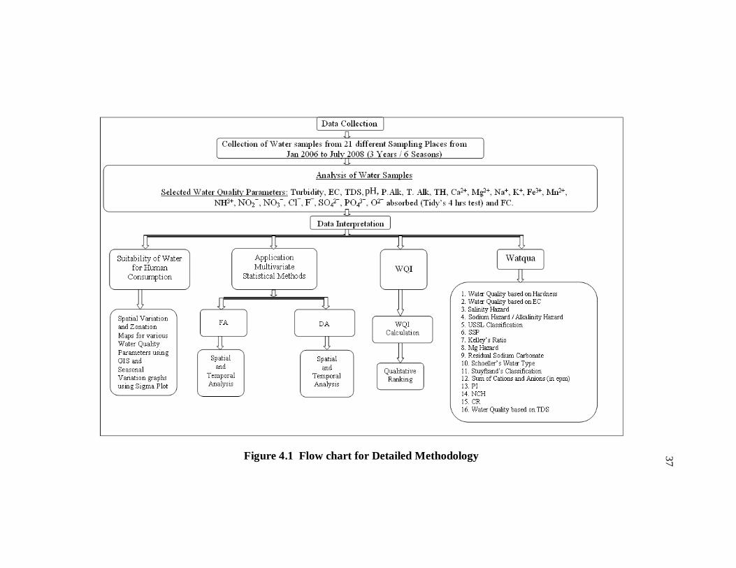
analyzed. The flow chart for detailed methodology is illustrated in

Figure 4.1.

37

Figure 4.1 Flow chart for Detailed Methodology

pH,

38

4.2 WATER QUALITY

Water quality refers to the chemical, physical and biological

characteristics of water. Water quality readings for rural areas which are in

and around SIPCOT industrial zone, Perundurai, Erode district were recorded.

The selected water quality parameters were (1) Turbidity (2) EC (3) TDS (4)

pH (5) P.Alk (6) T.Alk (7) TH (8) Ca2+ (9) Mg2+ (10) Na+ (11) K+ (12) Fe3+

(13) Mn2+ (14) NH3+ (15) NO2ˉ (16) NO3ˉ (17) Cl¯ (18) F¯

(19) SO42ˉ (20) PO4

3ˉ (21) O2ˉ absorbed (Tidy’s 4 hrs test) and (22) FC.

Sampling and water analysis were carried out as per APHA (1995), TWAD –

Lab manual (2000) and Trivedy and Goel (1986). The accuracy of the

chemical analysis was verified by calculating ion-balance errors which might

be around 10%. All the water quality parameters are expressed in mg/L,

except, pH, Turbidity (NTU), EC (S/cm) and FC (colonies/100 ml). These

parameters were specifically recorded to identify possible differences in the

water quality of this region.

4.3 SAMPLING PLACES

There is data for 21 water quality monitoring sites which are

situated in and around SIPCOT industrial zone, Perundurai, Erode district

having 22 water quality parameters over a period of 3 years (6 seasons – Jan

2006, July 2006, Jan 2007, July 2007, Jan 2008 and July 2008) were studied.

The details of sampling places are shown in Figure 4.2 and Table 4.1.

39

Figure 4.2 Details of Sampling Places

Table 4.1 Details of Sampling Places

Zone

Radial distance

from centre in Km

Sampling Code

Sample taken from

Depth (m)

Name of the

Village

I 1 D1 Dug Well 30.50 Elithingalpatti B1 Bore Well 106.70 Kuttam Palayam D2 Dug Well 18.30 Vettukattu Valasu

II 1.5 B2 Bore Well 91.50 Palaiya Kattur D3 Dug Well 27.50 Kuttap Palayam B3 Bore Well 122.00 Sengulam

III 2 B4 Bore Well 73.15 Kasilingam Palayam B5 Bore Well 183.00 Komara Palayam D4 Dug Well 24.40 Nelli Valasu

IV 3

B6 Bore Well 112.80 Kadappamadi B7 Bore Well 137.16 Saralai D5 Dug Well 21.34 Kambaliyam Patti D6 Dug Well 13.72 Varap Palayam S1 Surface Water - Odai Kattur S2 Surface Water - Ottandinayakkanpudur B8 Bore Well 183.00 Ingur

V Above 3

D7 Dug Well 25.90 Palap Palayam B9 Bore Well 76.20 Velliyam Palayam

B10 Bore Well 91.44 Koorai Palayam B11 Bore Well 21.34 Periyavettu Palayam S3 Surface Water - Palatholuvu

40

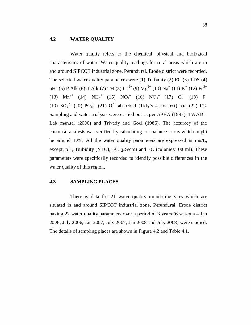
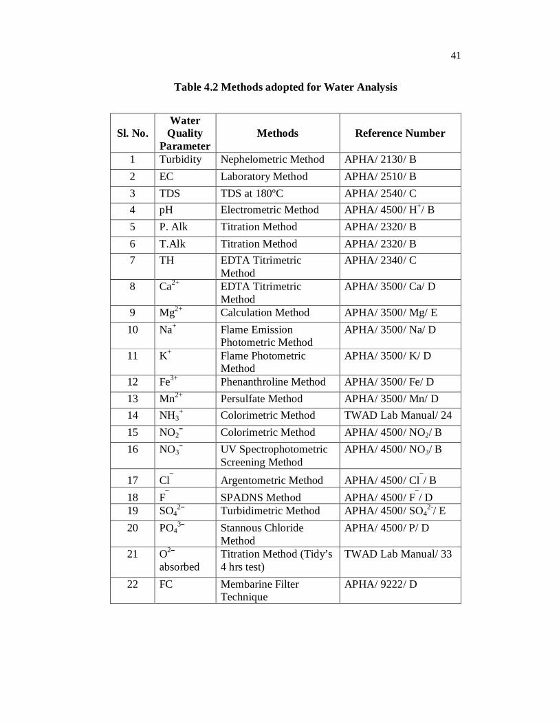
4.4 METHODS ADOPTED FOR WATER ANALYSIS

As the collected water samples are analyzed to determine the

concentrations of various water quality parameters, the adopted methods are

listed out in Table 4.2.

4.5 DATA ANALYSIS USING GIS

It may be advisable if one wants to map the water quality

parameters, the decision support like GIS can be used. GIS is an information

system which is generally designed for handling spatial data particularly.

Unlike manual cartographic analysis, GIS has advantage of handling attribute

data in conjunction with spatial features. To develop the study area map using

GIS, Survey of India topo-sheets (58 E/11 and 58 E/12) were used. Spatial

variation and zonation maps of various water quality parameters have been

developed by means of using GIS Package of Geomedia Professional 6.0.

They focus the pollution level of the study area related with water.

4.6 WATER QUALITY ASSESSMENT USING MULTIVARIATE

STATISTICAL METHODS

The water quality is mostly characterized by many variables

(parameters) which represent a water composition in specific localities and

time. Real hydrological data are mostly noisy. They are not normally

distributed, often co-linear or autocorrelated, containing outliers or errors etc.

These data sets create an n-dimensional space from which information about

the water composition has to be extracted. For this purpose, Multivariate

Methods such as FA and DA are used.

41

Table 4.2 Methods adopted for Water Analysis

Sl. No. Water

Quality Parameter

Methods Reference Number

1 Turbidity Nephelometric Method APHA/ 2130/ B 2 EC Laboratory Method APHA/ 2510/ B 3 TDS TDS at 180ºC APHA/ 2540/ C 4 pH Electrometric Method APHA/ 4500/ H+/ B 5 P. Alk Titration Method APHA/ 2320/ B 6 T.Alk Titration Method APHA/ 2320/ B 7 TH EDTA Titrimetric

Method APHA/ 2340/ C

8 Ca2+ EDTA Titrimetric Method

APHA/ 3500/ Ca/ D

9 Mg2+ Calculation Method APHA/ 3500/ Mg/ E 10 Na+ Flame Emission

Photometric Method APHA/ 3500/ Na/ D

11 K+ Flame Photometric Method

APHA/ 3500/ K/ D

12 Fe3+ Phenanthroline Method APHA/ 3500/ Fe/ D 13 Mn2+ Persulfate Method APHA/ 3500/ Mn/ D 14 NH3

+ Colorimetric Method TWAD Lab Manual/ 24 15 NO2ˉ Colorimetric Method APHA/ 4500/ NO2/ B 16 NO3ˉ UV Spectrophotometric

Screening Method APHA/ 4500/ NO3/ B

17 Cl¯ Argentometric Method APHA/ 4500/ Cl¯/ B 18 F¯ SPADNS Method APHA/ 4500/ F¯/ D 19 SO4

2ˉ Turbidimetric Method APHA/ 4500/ SO42-/ E

20 PO43ˉ Stannous Chloride

Method APHA/ 4500/ P/ D

21 O2ˉ absorbed

Titration Method (Tidy’s 4 hrs test)

TWAD Lab Manual/ 33

22 FC Membarine Filter Technique

APHA/ 9222/ D

42

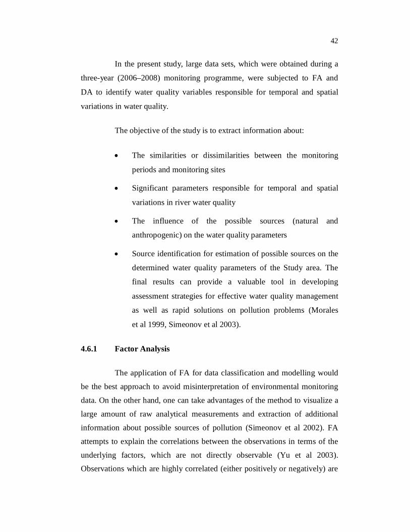
In the present study, large data sets, which were obtained during a

three-year (2006–2008) monitoring programme, were subjected to FA and

DA to identify water quality variables responsible for temporal and spatial

variations in water quality.

The objective of the study is to extract information about:

The similarities or dissimilarities between the monitoring

periods and monitoring sites

Significant parameters responsible for temporal and spatial

variations in river water quality

The influence of the possible sources (natural and

anthropogenic) on the water quality parameters

Source identification for estimation of possible sources on the

determined water quality parameters of the Study area. The

final results can provide a valuable tool in developing

assessment strategies for effective water quality management

as well as rapid solutions on pollution problems (Morales

et al 1999, Simeonov et al 2003).

4.6.1 Factor Analysis

The application of FA for data classification and modelling would

be the best approach to avoid misinterpretation of environmental monitoring

data. On the other hand, one can take advantages of the method to visualize a

large amount of raw analytical measurements and extraction of additional

information about possible sources of pollution (Simeonov et al 2002). FA

attempts to explain the correlations between the observations in terms of the

underlying factors, which are not directly observable (Yu et al 2003).

Observations which are highly correlated (either positively or negatively) are

43

influenced by the same factors, while those which are relatively uncorrelated,

are influenced by different factors. Environmetric methods including FA have

been used successfully in hydrochemistry for many years. If these techniques

are handled, it will be better to produce good result regarding surface water,

groundwater water quality assessment and environmental research. They

allow deriving hidden information from the data set about the possible

influences of the environment on water quality and offer greater possibilities

to managers in terms of aiding the decision making process (Lopez et al 2004,

Kotti et al 2005). The main objective of the method tells about determining:

The number of common factors influencing a set of

observations.

The strength of the relationship between each factor and each

observation (DeCoster 1998).

There are three stages in FA (Gupta et al 2005):

For all the variables, a correlation matrix is generated.

Initial set of factors are extracted. The factors are extracted

based on the fundamental theorem of FA, which says, that

every observed value can be written as a linear combination of

hypothetical factors. There are a number of different

extraction methods, including centroid, maximum likelihood,

principal component and principal axis extraction.

To maximize the relationship between some of the factors and

variables, the factors are rotated. By rotating, it is attempted to

find a factor solution that is equal to that obtained in the initial

extraction. Anyhow it has the simplest interpretation. The best

rotation method is widely believed to be Varimax. After a

Varimax rotation, each original variable tends to be associated

with one (or a small number) of factors and each factor

represents only a small number of variables.

44

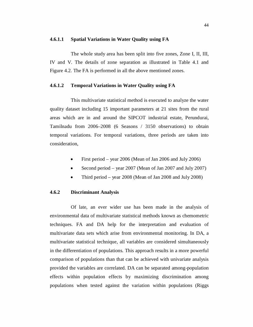
4.6.1.1 Spatial Variations in Water Quality using FA

The whole study area has been split into five zones, Zone I, II, III,

IV and V. The details of zone separation as illustrated in Table 4.1 and

Figure 4.2. The FA is performed in all the above mentioned zones.

4.6.1.2 Temporal Variations in Water Quality using FA

This multivariate statistical method is executed to analyze the water

quality dataset including 15 important parameters at 21 sites from the rural

areas which are in and around the SIPCOT industrial estate, Perundurai,

Tamilnadu from 2006–2008 (6 Seasons / 3150 observations) to obtain

temporal variations. For temporal variations, three periods are taken into

consideration,

First period – year 2006 (Mean of Jan 2006 and July 2006)

Second period – year 2007 (Mean of Jan 2007 and July 2007)

Third period – year 2008 (Mean of Jan 2008 and July 2008)

4.6.2 Discriminant Analysis

Of late, an ever wider use has been made in the analysis of

environmental data of multivariate statistical methods known as chemometric

techniques. FA and DA help for the interpretation and evaluation of

multivariate data sets which arise from environmental monitoring. In DA, a

multivariate statistical technique, all variables are considered simultaneously

in the differentiation of populations. This approach results in a more powerful

comparison of populations than that can be achieved with univariate analysis

provided the variables are correlated. DA can be separated among-population

effects within population effects by maximizing discrimination among

populations when tested against the variation within populations (Riggs

45

1973). Chemometric techniques are said to be useful to characterize the

quality of water and its “temporal and spatial variability caused by natural and

manmade factors” (Singh et al 2004). There are several methods available to

measure variations. With univariate analyses, each variable is analyzed

individually allowing for substantial overlapping of results to occur. DA was

applied to the raw dataset by using the standard and stepwise modes to

construct DFs to evaluate spatial and temporal variations in water quality. The

site (spatial) and season (temporal) were classified into the grouping

(dependent) variables, while the measured parameters constituted the

independent variables.

4.6.2.1 Spatial Variations in Water Quality using DA

For spatial analysis, there are two groups: (1) observations with low

TDS (Group I) and (2) observations with high TDS (Group II) were

categorized for Zone I, II, III, IV and V. The details of grouping for DA are

shown in Table 4.3. The selected parameters for the estimation of water

quality characteristics were: pH, T.Alk, TH, Ca2+, Mg2+, Na+, K+, Fe3+, NO3ˉ,

Cl¯, F¯, SO42ˉ, O2ˉ absorbed and FC.

4.6.2.2 Temporal Variations in Water Quality using DA

For temporal analysis, there are two groups: (1) observations with

low TDS (Group I) and (2) observations with high TDS (Group II) were

categorized for period I, II and III. The details of grouping for DA are shown

in Table 4.4. The selected parameters for the estimation of water quality

characteristics were: pH, total alkalinity, total hardness, calcium, magnesium,

sodium, potassium, iron, nitrate, chloride, fluoride, sulphate, oxygen absorbed

and faecal coliforms.

46

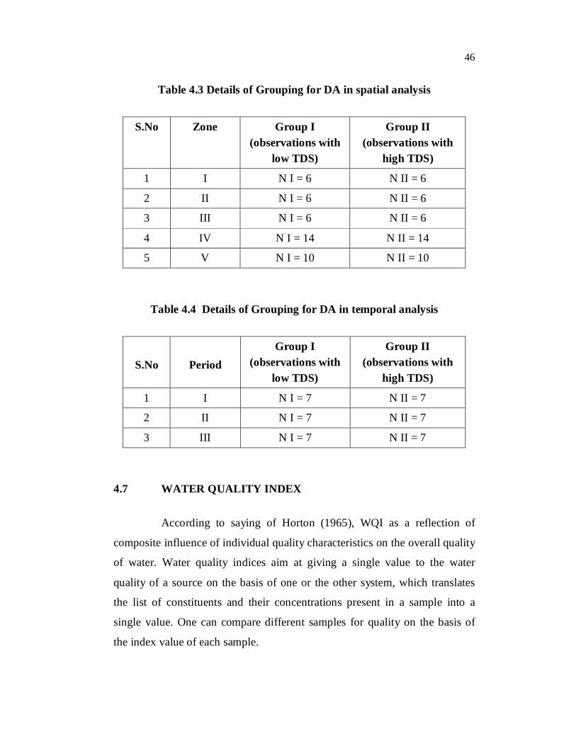
Table 4.3 Details of Grouping for DA in spatial analysis

S.No Zone Group I (observations with

low TDS)

Group II (observations with

high TDS)

1 I N I = 6 N II = 6

2 II N I = 6 N II = 6

3 III N I = 6 N II = 6

4 IV N I = 14 N II = 14

5 V N I = 10 N II = 10

Table 4.4 Details of Grouping for DA in temporal analysis

S.No

Period

Group I (observations with

low TDS)

Group II (observations with

high TDS)

1 I N I = 7 N II = 7

2 II N I = 7 N II = 7

3 III N I = 7 N II = 7

4.7 WATER QUALITY INDEX

According to saying of Horton (1965), WQI as a reflection of

composite influence of individual quality characteristics on the overall quality

of water. Water quality indices aim at giving a single value to the water

quality of a source on the basis of one or the other system, which translates

the list of constituents and their concentrations present in a sample into a

single value. One can compare different samples for quality on the basis of

the index value of each sample.

47

Water Quality Indices can be formulated in two ways: (1) Index

numbers increase with the degree of pollution (increasing scale indices) and

(2) index numbers decrease with the degree of pollution (decreasing scale

indices). One may classify the former as ‘water pollution indices’ and the

latter as ‘water quality indices’. But this difference appears as an essential

cosmetic: water quality is a general term, of which ‘water pollution’ that

indicates ‘undesirable water quality’ is a special case. In this study, water

quality indices with increasing scale indices were considered. Figure 4.3

illustrates how index values are calculated.

Figure 4.3 Process of WQI Calculation

48

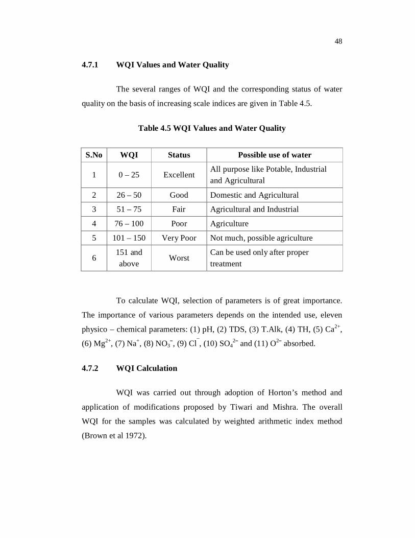
4.7.1 WQI Values and Water Quality

The several ranges of WQI and the corresponding status of water

quality on the basis of increasing scale indices are given in Table 4.5.

Table 4.5 WQI Values and Water Quality

S.No WQI Status Possible use of water

1 0 – 25 Excellent All purpose like Potable, Industrial and Agricultural

2 26 – 50 Good Domestic and Agricultural

3 51 – 75 Fair Agricultural and Industrial

4 76 – 100 Poor Agriculture

5 101 – 150 Very Poor Not much, possible agriculture

6 151 and above

Worst Can be used only after proper treatment

To calculate WQI, selection of parameters is of great importance.

The importance of various parameters depends on the intended use, eleven

physico – chemical parameters: (1) pH, (2) TDS, (3) T.Alk, (4) TH, (5) Ca2+,

(6) Mg2+, (7) Na+, (8) NO3ˉ, (9) Cl¯, (10) SO42ˉ and (11) O2ˉ absorbed.

4.7.2 WQI Calculation

WQI was carried out through adoption of Horton’s method and

application of modifications proposed by Tiwari and Mishra. The overall

WQI for the samples was calculated by weighted arithmetic index method

(Brown et al 1972).

49

4.7.2.1 Calculation of Unit Weight

Unit weight was calculated by a value inversely proportional to the

recommended Sn of the corresponding parameter.

kWnSn

(4.1)

where Wn - Unit weight for the nth parameters

Sn - Standard value of the nth parameter

k - Constant for proportionality

The water quality parameters and their unit weights (Wn) are

depicted in Table 4.6. The value of ‘k’ in each case is ‘0.823586’.

Table 4.6 Water quality parameters, their standard values, ideal

values and unit weights

S.No Parameters Standard

Value (Sn) Sn from

Ideal Value (Vid)

Unit Weight

1 TDS 500 IS 0 0.001647

2 pH 8.5 IS 7 0.096892

3 TAlk 120 ICMR 0 0.006863

4 TH 300 ICMR 0 0.002745

5 Ca2+ 75 IS 0 0.010981

6 Mg2+ 30 IS 0 0.027453

7 Na+ 200 WHO 0 0.004118

8 NO3ˉ 45 IS 0 0.018302

9 Cl¯ 250 ICMR 0 0.003294

10 SO42ˉ 200 IS 0 0.004118

11 O2ˉ

absorbed 1 IS 0 0.823586

50

4.7.2.2 Calculation of Quality Rating (qn)

Let there be n water quality parameters and qn corresponding to the

nth parameter is a number reflecting the relative value of this parameter in the

polluted water with respect to its standard permissible value. The qn is

calculated using the following expression.

nVn Vidq 100Sn Vid

(4.2)

where qn - Quality rating for the nth water quality parameter

Vn - Estimated value of the nth parameter at a given sampling

station

Sn - Standard permissible value of the nth parameter

Vid - Ideal value of nth parameter in pure water

(i.e. 7.0 for pH and 0 for all other parameters)

4.7.2.3 Calculation of WQI

The overall WQI was calculated by aggregating the qn with the unit

weight linearly.

nq WnWQI

Wn

(4.3)

4.8 WATQUA

In the age of modern technology, technical experts are ambitious of

inventing new things. Computer helps us in many ways to reduce our work-

burden while it gives perfect analysis. Similarly, “Watqua” is a new package

developed for this thesis using Visual Basic. This package about water quality

assessment can be performed at the fastest rate without applying tedious

51

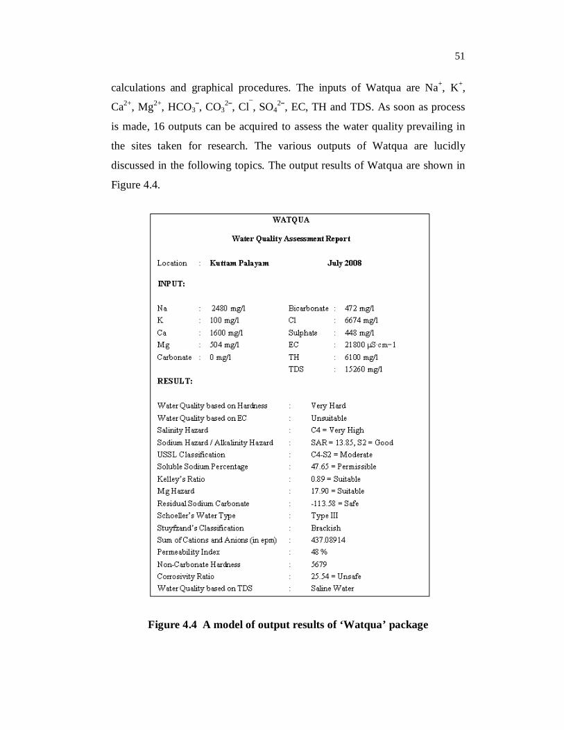
calculations and graphical procedures. The inputs of Watqua are Na+, K+,

Ca2+, Mg2+, HCO3ˉ, CO32ˉ, Cl¯, SO4

2ˉ, EC, TH and TDS. As soon as process

is made, 16 outputs can be acquired to assess the water quality prevailing in

the sites taken for research. The various outputs of Watqua are lucidly

discussed in the following topics. The output results of Watqua are shown in

Figure 4.4.

Figure 4.4 A model of output results of ‘Watqua’ package

52

4.8.1 First Output

Water quality based on hardness is the first output. Hardness is an

important criterion for determining the usability of water for domestic and

industrial purposes.

Classification of water based on the same is presented in Table 4.7

(Sawyer et al 1967).

Table 4.7 Water Quality based on Hardness

Sl. No TH (mg/L) Water Class

1 0 - 75 Soft

2 76 - 150 Moderately Hard

3 151 - 300 Hard

4 Above 300 Very Hard

4.8.2 Second Output

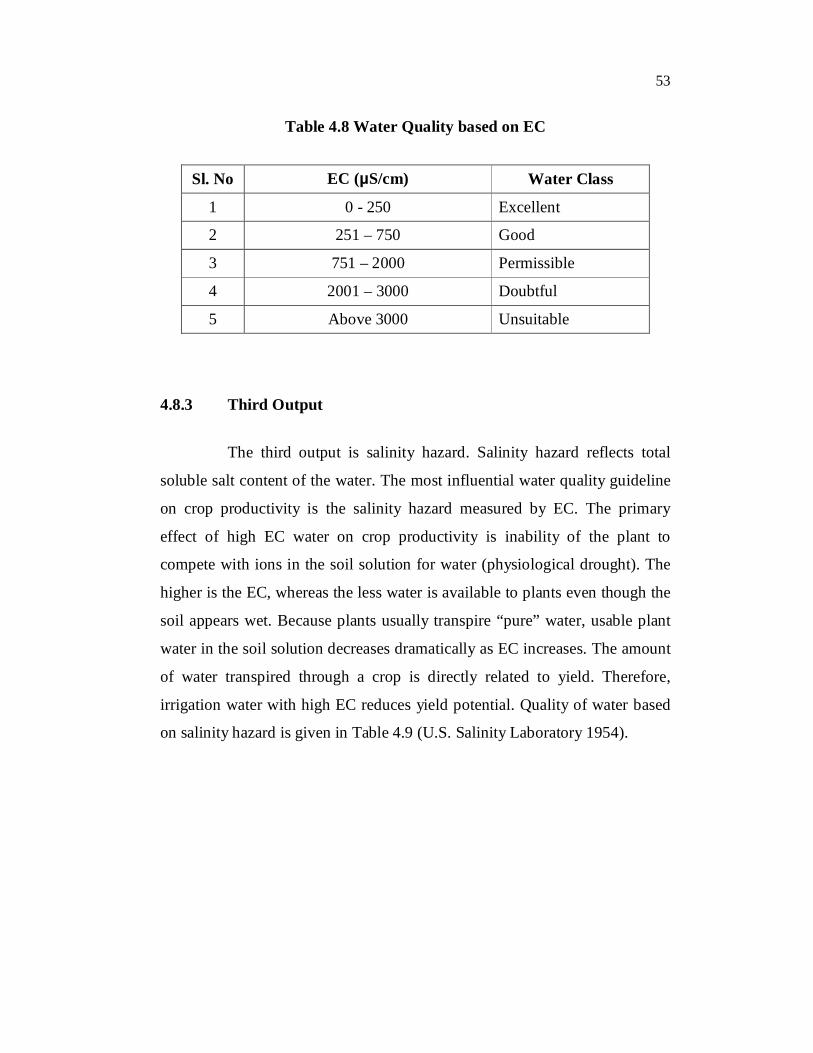
The Second output is nothing but water quality based on EC. The

total concentration of salts in irrigation water is measured by the electrical

current conducted by the ions in solution. EC is a good measure of salinity

hazard to crops as it reflects the TDS in groundwater. Quality of water based

on EC is given in Table 4.8 (Ragunath 1987).

53

Table 4.8 Water Quality based on EC

Sl. No EC (µS/cm) Water Class

1 0 - 250 Excellent

2 251 – 750 Good

3 751 – 2000 Permissible

4 2001 – 3000 Doubtful

5 Above 3000 Unsuitable

4.8.3 Third Output

The third output is salinity hazard. Salinity hazard reflects total

soluble salt content of the water. The most influential water quality guideline

on crop productivity is the salinity hazard measured by EC. The primary

effect of high EC water on crop productivity is inability of the plant to

compete with ions in the soil solution for water (physiological drought). The

higher is the EC, whereas the less water is available to plants even though the

soil appears wet. Because plants usually transpire “pure” water, usable plant

water in the soil solution decreases dramatically as EC increases. The amount

of water transpired through a crop is directly related to yield. Therefore,

irrigation water with high EC reduces yield potential. Quality of water based

on salinity hazard is given in Table 4.9 (U.S. Salinity Laboratory 1954).

54

Table 4.9 Water Quality based on Salinity Hazard

Sl. No. Symbol EC (µS/cm) Water Class Usage

1 C1 0 - 250 Low

Can be used for irrigation on most crops in most soils with little likelihood that soil salinity will develop.

2 C2 251 - 750 Medium Can be used if a moderate amount of leaching occurs.

3 C3 751 - 2250 High Cannot be used on soils with restricted drainage.

4 C4 Above 2250 Very High

Not suitable for irrigation under ordinary conditions, but it may be used occasionally under very special circumstances.

4.8.4 Fourth Output

The fourth output is sodium / alkalinity hazard. The sodium hazard

is typically expressed as the SAR. The formula for calculating SAR is shown

in equation (4.4).

SAR =2 2

NaCa Mg

2

(4.4)

where all ionic concentrations are expressed in meq/L.

55

This index quantifies the proportion of Na+ to Ca2+ and Mg2+ ions in

a sample. Ca2+ will flocculate (hold together), while Na+ disperses (pushes

apart) soil particles. This dispersed soil becomes crust and produces water

infiltration and permeability problems. General classifications of irrigation

water based upon SAR values are presented in Table 4.10 (Ragunath 1987).

Table 4.10 Water Quality based on Sodium / Alkalinity Hazard

Sl. No. Symbol SAR Water Class Usage

1 S1 0 - 10 Excellent

Can be used for irrigation on almost all soils with little danger of developing harmful levels of sodium.

2 S2 11 - 18 Good

May cause an alkalinity problem in fine-textured soils under low leaching conditions. It can be used on coarse textured soils with good permeability.

3 S3 19 - 26 Doubtful

May produce an alkalinity problem. This water requires special soil management such as good drainage, heavy leaching, and possibly the use of chemical amendments such as gypsum.

4 S4 Above 26 Unsuitable Usually unsatisfactory for irrigation purposes.

56

4.8.5 Fifth Output

The fifth output is USSL classification. In order to study the

suitability of water for irrigational uses, the values of EC and SAR are

compared and plotted on U.S. Salinity Laboratory diagram, which gives direct

indication of the salinity and alkali hazards. Classifications of irrigation water

based upon USSL are presented in Table 4.11 (U.S.Salinity Laboratory 1954).

Table 4.11 USSL Classification

Sl. No USSL Classification Water Class

1

C1 – S1 C2 – S2 C3 – S1 C4 – S1

Good

2

C1 – S2 C2 – S2 C3 – S2 C4 – S2

Moderate

3

C1 – S3 C2 – S3 C3 – S3 C4 – S3

Bad

4

C1 – S4 C2 – S4 C3 – S4 C4 – S4

Bad

57

4.8.6 Sixth Output

The sixth output is SSP. Wilcox (1955) has recommended

classification for rating irrigation water on the basis of soluble sodium

percentage. It is expressed in the equation (4.5).

SSP = 2 2

(Na K )Ca Mg Na K

× 100 (4.5)


Classifications of irrigation water based upon SSP are presented in

Table 4.12.

Table 4.12 Water Quality based on SSP

Sl. No SSP Water Class

1 0 - 20 Excellent

2 21 - 40 Good

3 41 - 60 Permissible

4 61 - 80 Doubtful


4.8.7 Seventh Output

The seventh output is Kelly’s Ratio. The formula used in the

estimation of this ratio is expressed in equation (4.6) (Kelly et al 1940).

Kelly’s Ratio = 2 2

NaCa Mg

(4.6)


58

Classifications of irrigation water based upon Kelly’s Ratio are

presented in Table 4.13.

Table 4.13 Water Quality based on Kelly’s Ratio

Sl. No Kelly’s Ratio Water Class

1 0 - 1 Suitable

2 1 – 2 Marginal


4.8.8 Eighth Output

The eighth output is magnesium hazard. Paliwal (1972) used the

ratio as an index of magnesium hazards for irrigation water. Table 4.14 shows

the range of Mg Hazards in water samples. The formula used in the estimation

of this ratio is expressed in equation (4.7).

Mg Hazards =2

2 2

Mg 100Ca Mg Na K

(4.7)


Table 4.14 Water Quality based on Magnesium Hazard

Sl. No Magnesium Hazard (%) Water Class

1 0 - 50 Suitable

2 51 - 65 Marginal


59

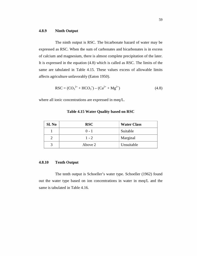
4.8.9 Ninth Output

The ninth output is RSC. The bicarbonate hazard of water may be

expressed as RSC. When the sum of carbonates and bicarbonates is in excess

of calcium and magnesium, there is almost complete precipitation of the later.

It is expressed in the equation (4.8) which is called as RSC. The limits of the

same are tabulated in Table 4.15. These values excess of allowable limits

affects agriculture unfavorably (Eaton 1950).

RSC = (CO32ˉ + HCO3ˉ) – (Ca2+ + Mg2+) (4.8)


Table 4.15 Water Quality based on RSC

Sl. No RSC Water Class

1 0 - 1 Suitable

2 1 - 2 Marginal


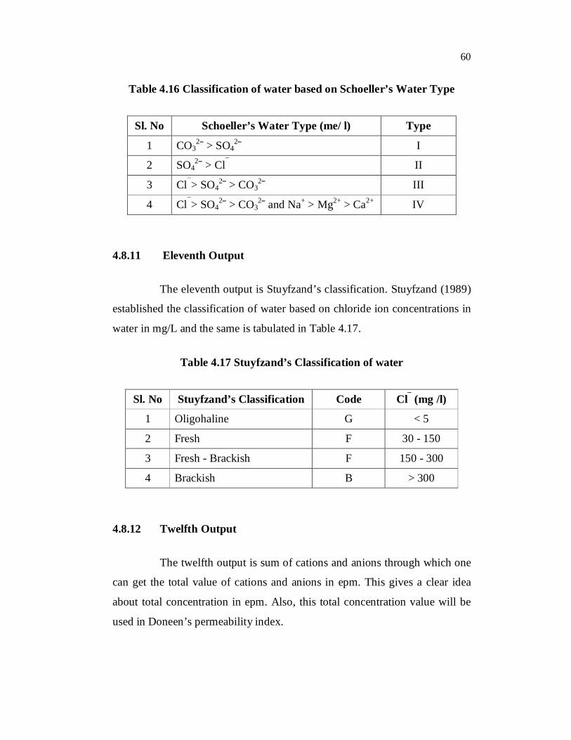
4.8.10 Tenth Output

The tenth output is Schoeller’s water type. Schoeller (1962) found

out the water type based on ion concentrations in water in meq/L and the

same is tabulated in Table 4.16.

60

Table 4.16 Classification of water based on Schoeller’s Water Type

Sl. No Schoeller’s Water Type (me/ l) Type

1 CO32ˉ > SO4

2ˉ I

2 SO42ˉ > Cl¯ II

3 Cl¯> SO42ˉ > CO3

2ˉ III

4 Cl¯> SO42ˉ > CO3

2ˉ and Na+ > Mg2+ > Ca2+ IV

4.8.11 Eleventh Output

The eleventh output is Stuyfzand’s classification. Stuyfzand (1989)

established the classification of water based on chloride ion concentrations in

water in mg/L and the same is tabulated in Table 4.17.

Table 4.17 Stuyfzand’s Classification of water

Sl. No Stuyfzand’s Classification Code Cl¯ (mg /l)

1 Oligohaline G < 5

2 Fresh F 30 - 150

3 Fresh - Brackish F 150 - 300

4 Brackish B > 300

4.8.12 Twelfth Output

The twelfth output is sum of cations and anions through which one

can get the total value of cations and anions in epm. This gives a clear idea

about total concentration in epm. Also, this total concentration value will be

used in Doneen’s permeability index.

61

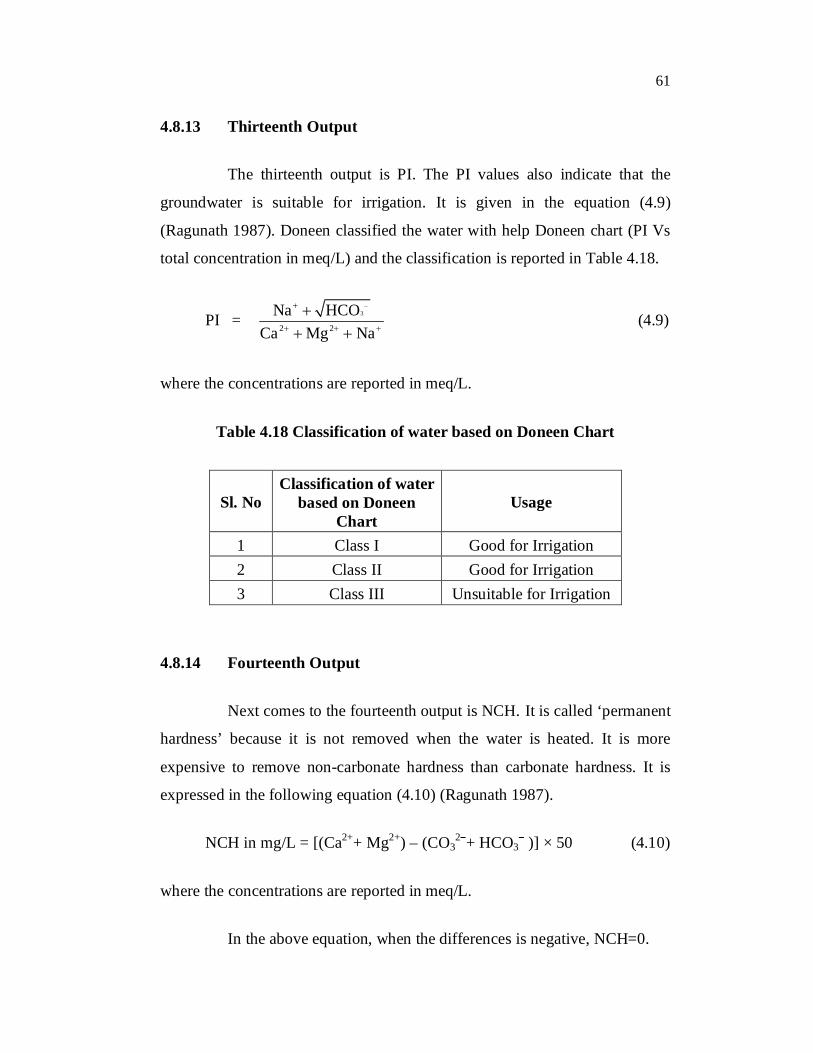
4.8.13 Thirteenth Output

The thirteenth output is PI. The PI values also indicate that the

groundwater is suitable for irrigation. It is given in the equation (4.9)

(Ragunath 1987). Doneen classified the water with help Doneen chart (PI Vs

total concentration in meq/L) and the classification is reported in Table 4.18.

PI = 3

2 2

Na HCOCa Mg Na

(4.9)

where the concentrations are reported in meq/L.

Table 4.18 Classification of water based on Doneen Chart

Sl. No Classification of water

based on Doneen Chart

Usage

1 Class I Good for Irrigation 2 Class II Good for Irrigation 3 Class III Unsuitable for Irrigation

4.8.14 Fourteenth Output

Next comes to the fourteenth output is NCH. It is called ‘permanent

hardness’ because it is not removed when the water is heated. It is more

expensive to remove non-carbonate hardness than carbonate hardness. It is

expressed in the following equation (4.10) (Ragunath 1987).

NCH in mg/L = [(Ca2++ Mg2+) – (CO32ˉ+ HCO3ˉ )] × 50 (4.10)


In the above equation, when the differences is negative, NCH=0.

62

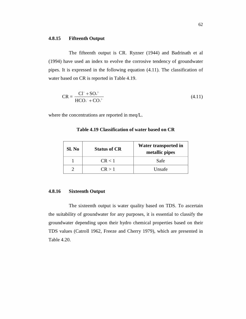
4.8.15 Fifteenth Output

The fifteenth output is CR. Ryzner (1944) and Badrinath et al

(1994) have used an index to evolve the corrosive tendency of groundwater

pipes. It is expressed in the following equation (4.11). The classification of

water based on CR is reported in Table 4.19.

CR = 2

4

23 3

Cl SOHCO CO

(4.11)


Table 4.19 Classification of water based on CR

Sl. No Status of CR Water transported in

metallic pipes

1 CR < 1 Safe

2 CR > 1 Unsafe

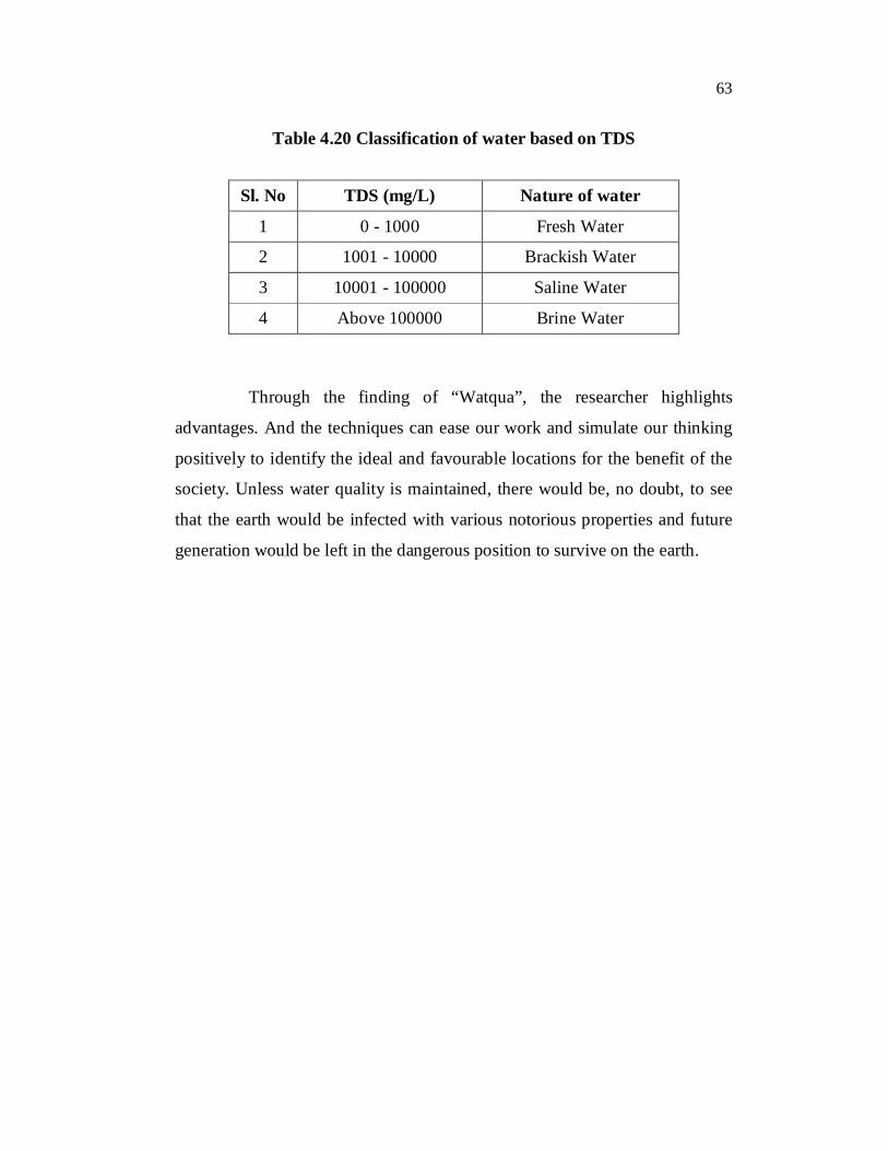
4.8.16 Sixteenth Output

The sixteenth output is water quality based on TDS. To ascertain

the suitability of groundwater for any purposes, it is essential to classify the

groundwater depending upon their hydro chemical properties based on their

TDS values (Catroll 1962, Freeze and Cherry 1979), which are presented in

Table 4.20.

63

Table 4.20 Classification of water based on TDS

Sl. No TDS (mg/L) Nature of water

1 0 - 1000 Fresh Water

2 1001 - 10000 Brackish Water

3 10001 - 100000 Saline Water

4 Above 100000 Brine Water

Through the finding of “Watqua”, the researcher highlights

advantages. And the techniques can ease our work and simulate our thinking

positively to identify the ideal and favourable locations for the benefit of the

society. Unless water quality is maintained, there would be, no doubt, to see

that the earth would be infected with various notorious properties and future

generation would be left in the dangerous position to survive on the earth.

chapter 4 materials and methods -...

Documents