Chapter 4 - Solution of

Nonlinear Equations

4.1 The Bisection Method

In this chapter, we will be interested in solvingequations of the form

f(x) = 0.

Because f(x) is not assumed to be linear, it could haveany number of solutions, from 0 to ∞.

In one dimension, if f(x) is continuous, we canmake use of the Intermediate Value Theorem (IVT)to bracket a root; i.e., we can find numbers a and bsuch that f(a) and f(b) have different signs.

Then the IVT tells us that there is at least one magicalvalue x∗ ∈ (a, b) such that f(x∗) = 0.

The number x∗ is called a root or zero of f(x).

Solving nonlinear equations is also called root-finding.

1

To “bisect” means to divide in half.

Once we have an interval (a, b) in which we know x∗lies, a systematic way to proceed is to sample f(a+b2 ).

If f(a+b2 ) = 0, then x∗ =a+b2 , and we are done!

Otherwise, the sign of f(a+b2 ) will either agree withthe sign of f(a), or it will agree with the sign of f(b).

Suppose the signs of f(a+b2 ) and f(a) agree.

Then we are no longer guaranteed that x∗ ∈ (a, a+b2 ),

but we are still guaranteed that x∗ ∈ (a+b2 , b).

So we have narrowed down the region where x∗ lies.

Moreover, we can repeat the process by setting a+b2 to

a (or to b, as applicable) until the interval containingx∗ is small enough.

See bisectionDemo.m

Interval bisection is a slow-but-sure algorithm forfinding a zero of f(x), where f(x) is a real-valuedfunction of a single real variable.

2

We assume that we know an interval [a, b] on which acontinuous function f(x) changes sign.

However, there is likely no floating-point number (oreven rational number!) where f(x) is exactly 0.

So our goal is:

Find a (small) interval (perhaps as small as 2 successivefloating-point numbers) on which f(x) changes sign.

Sadly, bisection is slow !

It can be shown that bisection only adds 1 bit ofprecision per iteration.

Starting from 0 bits of accuracy, it always takes 52steps to narrow the interval in which x∗ lies down to 2adjacent floating-point numbers.

However, bisection is completely foolproof .

If f(x) is continuous and we have a starting interval onwhich f(x) changes sign, then bisection is guaranteedto reduce that interval to two successive floating-pointnumbers that bracket x∗.

3

4.2 Newton’s Method

Newton’s method for solving f(x) = 0 works in thefollowing fashion.

Suppose you have a guess xn for a root x∗.

Find the tangent line to y = f(x) at x = xn andfollow it down until it crosses the x-axis; call thecrossing point xn+1.

This leads to the iteration

xn+1 = xn −f(xn)

f ′(xn).

Often xn+1 will be closer to x∗ than xn was.

Repeat the process until we are close enough to x∗.

See newtonDemo.m

When Newton’s method works, it is really great!

4

In fact, the generalization of the above description ofNewton’s method is the only viable general-purposemethod to solve systems of nonlinear equations.

But, as a general-purpose algorithm for finding zerosof functions, it has 3 serious drawbacks.

1. The function f(x) must be smooth.

2. The derivative f ′(x) must be computed.

3. The starting guess must be “sufficiently accurate”.

• If f(x) is not smooth, then f ′(x) does not exist, andNewton’s method is not defined.

Estimating or approximating derivative values at pointsof non-smoothness can be hazardous.

• Computing f ′(x) may be problematic.

Nowadays, the computation of f ′(x) can (in principle)be done using automatic differentiation:

5

Suppose we have a function f(x) and some computercode (in any programming language) to evaluate it.

By combining modern computer science parsingtechniques with the rules of calculus (in particular thechain rule), it is theoretically possible to automaticallygenerate the code for another function, fprime(x),that computes f ′(x).

You may be able to use software that estimates f ′(x)by means of finite differences; e.g.,

f ′(x) ≈ f(x+ ε)− f(x− ε)2ε

.

If we could take limε→0 of the right-hand side, thenwe would precisely have f ′(x). (Why can’t we?)

But it still may be expensive or inconvenient dependingon your computing environment.

• If x0 is not sufficiently accurate, Newton’s methodwill diverge (often catastrophically!).

6

The local convergence properties of Newton’s methodare its strongest features.

Let x∗ be a zero of f(x), and let en = x∗ − xn be theerror in the nth iterate.

Assume

• f ′(x) and f ′′(x) exist and are continuous.

• x0 is sufficiently close to x∗.

Then it is possible to prove that

en+1 =1

2

f ′′(ξ)

f ′(xn)e2n,

where ξ is some point between xn and x∗.

In other words, the new error is roughly the size of thesquare of the old error.

(In this case we say en+1 = O(e2n).)

7

This is called quadratic convergence:

For nice,1 smooth functions, once xn is close enoughto x∗, the error goes down roughly by its square witheach iteration.

=⇒ The number of correct digits approximatelydoubles with each iteration!

(This is much faster than bisection, which only haslinear convergence.)

The behaviour we saw for computing√x is typical.

Beware! When the assumptions underlying the localconvergence theory are not satisfied, Newton’s methodmight not work.

If f ′(x) and f ′′(x) are not continuous and bounded, orif x0 is not “close enough” to x∗, then the local theorydoes not apply!

→ We might get slow convergence, or even noconvergence at all.

1By “nice”, here we mean f(x) such that f ′′(x) is bounded andf ′(x∗) 6= 0.

8

4.3 Bad Behaviour of Newton’s Method

As we have indicated, Newton’s method does notalways work.

Potentially bad behaviour of Newton’s method includes

• convergence to an undesired root,

• periodic cycling,

• catastrophic failure.

9

• It is easy to see geometrically how Newton’s methodcan converge to a root that you were not expecting.

Let f(x) = x2 − 1.

This function has 2 roots: x = −1 and x = 1.

From the graph of f(x) and the geometricinterpretation of Newton’s method, we see that wewill get convergence to x = −1 for any x0 < 0 and tox = 1 for any x0 > 0.

(Newton’s method is undefined in this case for x0 = 0.)

10

• To see how Newton’s method can cycle periodically,we have to cook up the right problem.

Suppose we want to see Newton’s method cycle abouta point a.

Then the iteration will satisfy

xn+1 − a = a− xn.

Therefore, we write

x− f(x)

f ′(x)− a = a− x,

and solve this equation for the evil f(x):

df

f=

dx

2(x− a).

11

Integrating both sides,

ln |f(x)| = 1

2ln |x− a|+ C,

where C is an arbitrary constant, or

|f(x)| = A√|x− a|,

where A = eC. Noting

f(x) = ±A√|x− a|,

we can choose A = sgn(x− a).

12

Here is a plot of the f(x) and the cyclic behaviour fora = 2 and x0 = 3 or −1.

0 0.5 1 1.5 2 2.5 3 3.5 4

−1.5

−1

−0.5

0

0.5

1

1.5

x

sign(x−2) sqrt(abs(x−2))

Of course, x∗ = a.

What goes wrong?

The local convergence theory for Newton’s methodfails for this problem because f ′(x) is unbounded asx→ a.

13

• Newton’s method can fail completely.

When it does, it is usually in a catastrophic fashion;i.e., the iterates xn become numerically unbounded inonly a few iterations.

(And if you are watching the iterates as they arecomputed, it becomes clear within an iteration or twothat things aren’t going to work.)

This bad behaviour is much more common whensolving systems of nonlinear equations, so we defermore discussion until the end of this chapter.

What this tells us however is that having a goodguess is even more important when solving a system ofnonlinear equations.

(Unfortunately, it is also much harder to obtain one!)

For scalar equations, the problem of catastrophic failuregenerally stems from having f ′(xn) “point in the wrongdirection”.

14

In practice, to enhance the global convergenceproperties of Newton’s method, only part of theNewton “step” is taken when xn is “far” from x∗:

The iteration is modified to

xn+1 = xn−λnf(xn)

f ′(xn).

A computation is performed to compute a scalingfactor λn ∈ (0, 1] that tells us what fraction of theNewton correction to take.

As xn → x∗, λn → 1;

i.e., as we approach the solution, we tend to take thewhole Newton step (and get quadratic convergence).

This is called the damped Newton method.

The idea is that far from the root, you would not takethe whole Newton step if it is bad (and hence avoidcatastrophic failure).

15

Some other safeguards that are also added to softwarein practice to allow for graceful termination of thealgorithm:

• Specify a maximum number of iterations allowed.

• Check that the Newton correction f(xn)/f′(xn) is

not too large (or alternatively λn is not too small).

16

4.4 The Secant Method

One of the greatest shortcomings of Newton’s methodis that it requires the derivative f ′(x) of the functionf(x) whose root we are trying to find.

The secant method replaces the derivative evaluation inNewton’s method with a finite difference approximationbased on the two most recent iterates.

Geometrically, instead of drawing a tangent to f(x)at the current iterate xn, you draw a straight line(secant) through the two points (xn, f(xn)) and(xn−1, f(xn−1)).

The next iterate xn+1 is again the intersection of thissecant with the x-axis.

The iteration requires two starting values, x0 and x1.

17

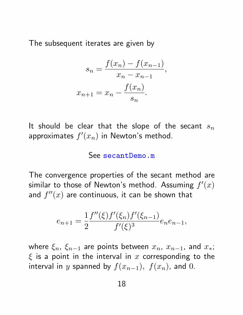
The subsequent iterates are given by

sn =f(xn)− f(xn−1)

xn − xn−1,

xn+1 = xn −f(xn)

sn.

It should be clear that the slope of the secant snapproximates f ′(xn) in Newton’s method.

See secantDemo.m

The convergence properties of the secant method aresimilar to those of Newton’s method. Assuming f ′(x)and f ′′(x) are continuous, it can be shown that

en+1 =1

2

f ′′(ξ)f ′(ξn)f′(ξn−1)

f ′(ξ)3enen−1,

where ξn, ξn−1 are points between xn, xn−1, and x∗;ξ is a point in the interval in x corresponding to theinterval in y spanned by f(xn−1), f(xn), and 0.

18

This is not quadratic convergence, but it is superlinearconvergence.

It can be shown that

en+1 = O(eφn),

where φ = (1 +√5)/2 ≈ 1.6 is the golden ratio.

In other words, when xn gets close to x∗, the numberof correct digits is multiplied by φ with each iteration.

That’s almost as fast as Newton’s method!

It is a great deal faster than bisection.

Typically, the secant method is very popular becausealthough the convergence rate is not as fast as thatof Newton’s method (and so you need a few moreiterations to reach a given accuracy), a secant iterationis usually much cheaper than a Newton iteration.

This means that ultimately the secant method isactually faster than Newton’s method to find a rootto a given accuracy.

19

4.5 Inverse Quadratic Interpolation

A typical train of thought in numerical analysis is thefollowing.

We notice that the secant method uses 2 previouspoints xn, xn−1 in determining the next one, xn+1.

So we begin to wonder: is there anything to be gainedby using 3 points?

Suppose we have 3 values, xn, xn−1, and xn−2, andtheir corresponding function values, f(xn), f(xn−1),and f(xn−2).

We could interpolate these values by a parabola andtake xn+1 to be the point where the parabola intersectsthe x-axis.

Problem: The parabola might not intersect the x-axis!

(This is because a quadratic function does notnecessarily have real roots.)

20

Note: This could be regarded as an advantage!

In fact an algorithm known as Muller’s methoduses the complex roots of the quadratic to produceapproximations to complex zeros of f(x).

Unfortunately, we have to avoid complex arithmetic.

So instead of a quadratic in x, we interpolate the 3points with a quadratic function in y!

This leads to a sideways parabola, P (y), determinedby the interpolation conditions

xn = P (f(xn)), xn−1 = P (f(xn−1)), xn−2 = P (f(xn−2)).

Note: We are reversing the traditional roles of thedata x and y in this process!

A sideways parabola always hits the x-axis (y = 0).

So, xn+1 = P (0) is the next iterate.

21

This method is known as inverse quadraticinterpolation (IQI).

The biggest problem with this “pure” IQI algorithm isthat polynomial interpolation assumes the x data (alsocalled the abscissae), which in this case are f(xn),f(xn−1), and f(xn−2), to be distinct.

Doing things as we propose, we have no guarantee thatthey will be!

For example, suppose we want to compute√2 using

f(x) = x2 − 2.

If our initial guesses are x0 = −2, x1 = 0, x2 = 2,then f(x0) = f(x2) and x3 is undefined!

Even if we start near this singular situation, e.g., withx0 = −2.001, x1 = 0, x2 = 1.999, then x3 ≈ 500.

Cleve likens IQI to an immature race horse: It movesvery quickly when it is near the finish line, but itsoverall behavior can be erratic.

→ It needs a good trainer to keep it under control.

22

4.6 The Zero-in Algorithm

The zero-in algorithm is a hybrid algorithm thatcombines the reliability of bisection with the speedof secant and IQI.

The algorithm was first proposed by Dekker in the1960s. It was later refined by Brent (1973).

The steps of the algorithm are as follows.

23

• Start with points a, b so that f(a), f(b) haveopposite signs, |f(b)| ≤ |f(a)|, and c = a.

• Use a secant step to give b+ between a and b.

• Repeat the following steps until |b−a| < εmachine|b|or f(b) = 0.

– Set a or b to b+ in such a way that∗ f(a) and f(b) have opposite signs;∗ |f(b)| ≤ |f(a)|;∗ Set c to the old b if b = b+; else set c = a.

– If c 6= a, consider an IQI step.– If c = a, consider a secant step.– If the result of the IQI or secant step is in the

interval [a, b], take it as the new b+.– If the step is not in the interval, use bisection to

get the new b+.

24

This algorithm is foolproof: It maintains in a shrinkinginterval that brackets the root.

It uses rapidly convergent methods when they arereliable; but it uses a slow-but-sure method whennecessary to maintain a bracket for the root andguarantee convergence.

This is the algorithm implemented in Matlab’s fzerofunction.

See fzeroDemo.m and fzerogui.m

25

Solving Systems of Nonlinear Equations

We now consider systems of nonlinear equations.

We are now looking for a solution vector x =(x1, x2, . . . , xm)

T that satisfies a set of m nonlinearequations f(x) = 0, where

f(x) =

f1(x1, x2, . . . , xm)f2(x1, x2, . . . , xm)

...fm(x1, x2, . . . , xm)

.

26

This case is much more difficult than the scalar casefor a number of reasons; e.g.,

• Much more complicated behaviour is possible,making analysis of existence and number of solutionsmuch harder or even impossible.

• There is no concept of bracketing in higherdimensions, so foolproof methods that areguaranteed to converge to the correct solution donot exist.

• Computational costs increase exponentially withincreasing dimension.

Consider the following system of 2 equations:

x21 − x2 + γ = 0,

−x1 + x22 + γ = 0,

where γ is a parameter.

27

Each equation defines a parabola, and the solutions (ifany) are the intersection points of these parabolas.

Depending on γ, this system can have 0, 1, 2, or 4solutions.

x

y

γ = 0.5

−2 −1 0 1 2−2

−1

0

1

2

x

y

γ = 0.25

−2 −1 0 1 2−2

−1

0

1

2

x

y

γ = −0.5

−2 −1 0 1 2−2

−1

0

1

2

x

y

γ = −1

−2 −1 0 1 2−2

−1

0

1

2

28

Newton’s Method

Many methods for finding roots in one dimension donot generalize directly to m dimensions.

Fortunately, Newton’s method can generalize to higherdimensions quite easily.

It is arguably the most popular and powerful methodfor solving systems of nonlinear equations.

Before discussing it, we will first need to introduce theconcept of the Jacobian matrix (also known as thematrix of first partial derivatives).

Let

f(x) =

f1(x1, x2, . . . , xm)f2(x1, x2, . . . , xm)

...fm(x1, x2, . . . , xm)

.

29

Then the Jacobian matrix Jf(x) =∂f(x)∂x is an m ×m

matrix whose (i, j) element is given by

[Jf(x)]ij =∂fi∂xj

.

e.g., when m = 2,

Jf(x) =

[∂f1∂x1

∂f1∂x2

∂f2∂x1

∂f2∂x2

].

Let

f(x) =

(x21 − x2 + γ−x1 + x22 + γ

).

Then,

Jf(x) =

[2x1 −1−1 2x2

].

30

The Newton iteration for systems of nonlinearequations takes the form

xn+1 = xn − Jf−1(xn)f(xn).

Of course, in practice we never actually form Jf−1(xn)!

Instead we solve the linear system

Jf(xn)sn = −f(xn),

then updatexn+1 = xn + sn.

→ Newton’s method reduces the solution of a nonlinearsystem to the solution of a sequence of linear equations.

31

Example

Solve the nonlinear system

f(x) =

[x1 + 2x2 − 2x21 + 4x22 − 4

]= 0.

First compute the Jacobian:

Jf(x) =

[1 22x1 8x2

].

Start with initial guess x0 = [1, 2]T .

Then,

f(x0) =

[313

], Jf(x0) =

[1 22 16

].

32

Solve for the correction s0 from[1 22 16

]s0 = −

[313

]=⇒ s0 =

[−1.83−0.58

].

So

x1 =

[12

]+

[−1.83−0.58

]=

[−0.831.42

],

etc.

If the process converges, we iterate until we havesatisfied some stopping criterion.

As a compromise between checking for absolute andrelative change in the iterates, we use a stoppingcriterion like

e = ‖xn+1 − xn‖+ 4εmachine‖xn+1‖,

and stop when e is less than some tolerance (say 10−8).

See systemDemo.m

33

Notes:

1. Newton’s method is quadratically convergent is mdimensions, but the proof is beyond the scope ofthis course.

2. The computational expense of solving a system ofm nonlinear equations can be substantial!→ computing Jf(x) requires m2 functionevaluations→ solving the linear systems by Gaussian eliminationcosts O(m3) operations

These statements assume that the Jacobian is dense.

If it is sparse or has some special structure or properties,some savings can usually be had.

34

Quasi-Newton Methods

These are also called secant-updating methods.

The main computational cost of Newton’s method inhigher dimensions is in evaluating the Jacobian andsolving the linear system

Jf(xn)sn = −f(xn).

There are 2 main ways to reduce this cost:

1. only update the Jacobian every few iterationsThis is known as freezing the Jacobian.If you store the LU factors from the first linearsystem solve, the cost of solving subsequent systemswith the frozen Jacobian is much less than theoriginal cost (O(m2) vs. O(m3)).If you only ever use Jf(x0), this is known as thechord method.It is the analogue of the secant method in higherdimensions.

35

2. build up an approximation to the Jacobian usingsuccessive iterates and function valuesThe most well-known of these methods is calledBroyden’s method.Unfortunately its description is beyond the scope ofthis course.

Again, more iterations are generally required of a quasi-Newton method compared to Newton’s method.

However, the cost of these extra iterations is usuallymore than made up for with savings in costs periteration.

Hence, there is often a net savings in using suchmethods over Newton’s method.

36