chapter 4 transportation environment surveys
TRANSCRIPT

Chap 4 Transportation Environment Surveys
4 - 1
Chapter 4 Transportation Environment Surveys
4.1 The Selection of the Cooperative Companies
During the first Site Survey of the first year, the cooperating companies have been pre-selected through the recommendations of the counterpart institutes of each Member Country. Based on this, the JICA Study Team decided to contact again the companies in order to explain the guidelines and details of the Study and to select the routes for surveys related to the products to be analyzed. Also, regarding to the Transportation Environment surveys, the details were given about the measuring devices to be used during the surveys (sensors and Global Positioning System GPS), the dummy cargoes for collecting impacts data and the work schedule as well.
The selected companies on each country are as follows: Argentina: Nucete e Hijos (Agro-aceitunera), Herederos de A. Williner SA, Frimetal SA Brazil: Multibras SA, BSH (Bosch und Siemens Hausgeräte), Klabin SA Paraguay: Cooperativa Chortitzer Komittee Uruguay: CONAPROLE (Cooperativa Nacional de Productores de Leche)
4.2 The Selection of the Distribution Routes for the Study
A series of meetings have been held between the JICA Study Team and the cooperating companies of the 4 countries, in order to discuss the details of the routes for surveys of the Study, and the work schedule as well.
For the first field surveys, it was defined the organization to be leaded by the JICA Study Team and with the participation of the members of the counterpart. The working groups have been divided to one per each country.
The target products for the surveys, classified by countries, are as follows: Argentina: Olive products, dairy products, refrigerators, edible oil Brazil: Refrigerators, air conditioning equipment (outdoor type) Paraguay: Dairy products Uruguay: Dairy products
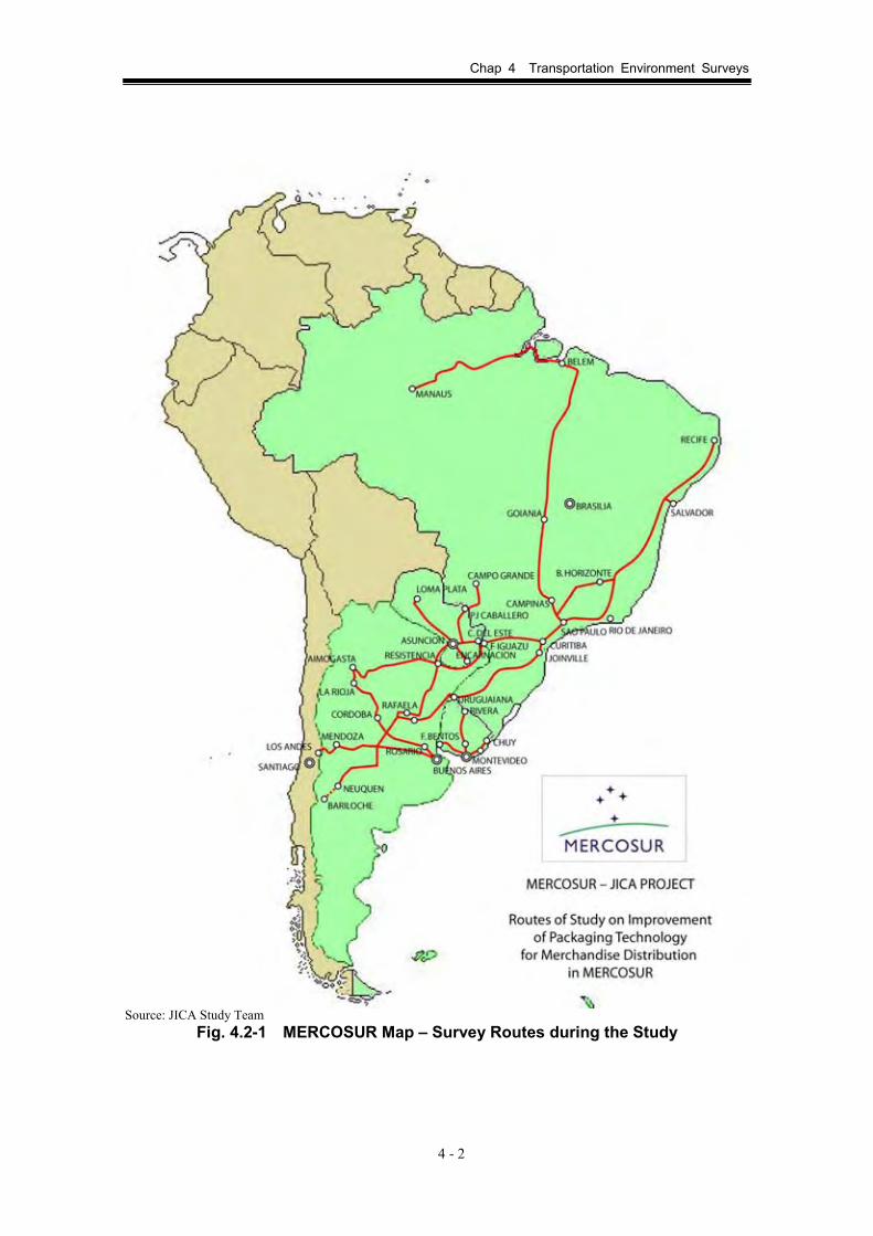
The routes studied during the Transportation Environment Surveys are indicated in the
following map and summary table (See Fig 4.2-1 and Table 4.2-1).
Chap 4 Transportation Environment Surveys
4 - 2
Source: JICA Study Team
Fig. 4.2-1 MERCOSUR Map – Survey Routes during the Study

Chap 4 Transportation Environment Surveys
4 - 3
Table 4.2-1 Transportation Environment Surveys, Routes and Itinerary
Original Plan Actual Plan Distance County Route Target
Product One way
Company Route Target Product Distance Company Date
Bs.As. - Aimogasuta
Processed Olive 1,200km NUCETE Bs.As. -
Aimogasta Processed Olive
2,500km (Round trip)
NUCETE 2/9 - 2/12 '05
Rafaela - Asunción
Powdered Milk 800km Willner Rafaela -
Asunción Powdered Milk
1,600km (Round trip)
Willner 7/3 - 7/7 '05
Aimogasta - Curitiba
Olive Product 2,500km NUCETE Aimogasta -
Curitiba Olive Product 2,500km NUCETE 7/19 - 7/23 '05
Rafaela - Neuquen
Dairy Product 1,300km Willner Rafaela -
Neuquen Dairy Product 1,800km Willner 7/8 - 7/12 '05
Neuquen-Santa Rosa
Only measurement 500km Williner 7/11 '05
Neuquen - Bariloche
Dummy Cargo Handling Survey
Willner Neuquen - Bariloche
Dummy Cargo Handling Survey
Willner
Dummy was improved for impact test after 3 months past
Aimogasta-Iguazú Olive Product 1,600km NUCETE 11/20-21 '05
Rosario - Mendoza - Santiago
Refrigerator, Showcase 1,500km FRIMETAL Cancelled because of Chile boarder closing due to heavy snow (’05)
Uruguaiana - Medoza - Los Andes
Refrigerator 1,700km Multibras Uruguaiana - Mendoza - Los Andes
Refrigerator 1,700km Multibras 10/11-20 '05
Rosario - Mendoza - Santiago
Refrigerator, Showcase 1,500km FRIMETAL Cancelled because of Chile boarder closing due to heavy snow (’06)
Bs.As. - Mendoza
Vegetable Oil 1,000km MOLINOS Bs.As. - Mendoza Vegetable Oil 1,000km MOLINOS 5/26 ‘06
Arge
ntina
Bs.As. - Rosario Refrigerator 300km FRIMETAL Bs.As. - Rosario Refrigerator 300km FRIMETAL
Several times including model projects in 2006
São Paulo - Recife Refrigerator 3,000km Multibras Joinville -
Salvador Refrigerator 2,500km Multibras 9/8 - 9/12 '05
Sã Paulo - Recife Refrigerator 3,000km BSH Campinas -
Recife Refrigerator 2,650km BSH 10/21 - 26 '05
Manaus - Belem - São Paulo
Refrigerator, Other Home Appliances
4,700km Multibras Manaus - Belem - São Paulo
Air Conditioner 4,700km Multibras 9/14 -
9/23
Braz
il
São Paulo - Uruguaiana - BsAs
Refrigerator 2,500km Multibras Joinville - Uruguaiana - Santiago
Refrigerator 2,700km Multibras 10/11 - 20 '05

Chap 4 Transportation Environment Surveys
4 - 4
Original Plan Actual Plan Distance County Route Target
Product One way
Company Route Target Product Distance Company Date
Loma Plata - P.J. Caballero
Dairy Product 800km Choritizer
Asunción - PJ Caballero - Campo Grande
Dairy Product 1,000km Chortizer 12-‘06
Asunción - Cd. del Este
Dairy Product 340km Choritizer
Loma Plata - Asunción - Cd. del Este
Dairy Product 860km Choritizer 9/27 - 28
'05
Asunción - Encarnación
Dairy Product 400km Choritizer
Loma Plata - Asunción Encarnación
Dairy Product 900km Choritizer 10/4 -
10/5
Gran Asunción Delivery
Dairy Product Choritizer 9/30 '05
Para
guay
Asunción City Delivery
Dairy Product Choritizer 10/14 '05
Florida - Montevideo
Butter, Powered Milk
100km Conaprole Rivera - Florida - Montevideo
Long Life Milk 4,800km Conaprole 9/8 - 9 '05
Montevideo - Chuy
Butter, Powered Milk
250km Conaprole Montevideo - Rocha
Long Life Milk 200km Conaprole
Several times in LATU Ur
ugua
y
Montevideo - Fray Bentos
Butter, Powered Milk
300km Conaprole Montevideo - Fray Bentos
Long Life Milk, Yoghurt, Cheese
400km Conaprole 9/5 ’05
Source: JICA Study Team Note): In Paraguay, the transportation environment surveys were implemented by INTN and Chortitzer during the
absence of the Study Team. 1. Loma Plata – Asunción; 550km (one-way)×6 times=3,300km 2. Loma Plata – Encarnación; 1,100km (one-way)×1 time 3. Asunción - Campo Grande (BRA); 1,000km(one-way)×1 time 4. Loma - Plata Ciudad del Este; 800km(one-way)×1 time

Chap 4 Transportation Environment Surveys
4 - 5
4.3 Data collection on the Transportation Environment Surveys
The Transportation Environment Surveys have been carried out in two stages. The first stage was developed as a Demonstration Test, using at this time DER-SMART sensors, and studying the return way of Buenos Aires - Aimogasta (La Rioja Province) in Argentina, separated 1,200km each other. On this survey, the products transported were packed with olives.
After that, in July 2005, it was carried out the first effective route survey with Williner company products (dairy products) and using the same type of sensors (DER-SMART).
The studied routes for this company are as follows: (1) Rafaela (Santa Fe Province) – Clorinda (Formosa Prov.) – Asuncion (Paraguay) (2) Rafaela (Santa Fe Province) – Neuquen (Neuquen Prov.) After that, in August 2005, a new training program was held in Asuncion (Paraguay) due to
incorporation of new type of sensors for the Study (SAVER 3X90), in order to allow the counterpart members of the 4 countries to be familiar with the handling and operation of the new devices.
On this stage of the Project, all the counterpart of the 4 Member Countries finally received the total lot of the measuring devices, so that the field survey activities started with full capacity from September 2005. This is the timing of starting the 2nd Stage of the Transportation Environment Surveys on routes. As result of the activities on this stage of the Study, in the case of Brazil, the surveys covered the following routes:
1) Joinville – Salvador (Bahia) 2) Manaus – Belem – San Pablo 3) Joinville – (through Argentina) - Santiago (Chile) 4) Hortlandia – Recife
In the case of Paraguay, the surveyed routes are 6: 1) Loma Plata - Asuncion 2) Loma Plata – Asuncion - Encarnacion 3) Loma Plata – Asuncion – Ciudad del Este 4) Gran Asuncion (Urban area) 5) Zona del Asuncion (suburban area) 6) Asuncion – Campo Grande
For the case of Uruguay, the studied routes are 5: 1) Montevideo – Rivera (2 surveys) 2) Montevideo – Rocha (2 surveys) 3) Montevideo – Fray Bentos

Chap 4 Transportation Environment Surveys
4 - 6
As result of all these surveys, a series of data have been collected by each country. These data have been processed for data analysis and it was obtained a group database.
The JICA Study Team compiled all the collected information into a common database. One copy of this database have been transferred to each counterpart institute during May-June 2006, by sending one unit of Hard Disk Drive (HDD) for each party.

Chap 4 Transportation Environment Surveys
4 - 7
4.4 Data Analysis of Collected Data
The analysis of collected data in the surveyed routes has been developed by the Study members, by applying the procedures recommended by the sensor’s manufacturers. For this purpose, it was necessary to standardize the data analysis procedures, so that it was prepared the “Data Analysis Procedure” both in Japanese and English, applicable for DER SMART sensors and SAVER3x90 separately.
4.4.1 Data Analysis Procedure for DER-SMART Sensors
The main topics of the data analysis procedure for DER-SMART sensors are described below. This procedure has been developed based on the survey of Rafaela (Santa Fe Prov.) – Asuncion (Paraguay) carried out on July 2005, where the surveyed product was dairy products of Williner company.
(1) Truck stopping point identification Procedure 1) By checking the G-S table, the truck stop points are identified and those events are
taken out. 2) By the table in which the stopping points are eliminated, the Grms – Speed curves are
plotted (Fig. 4.4-1).
Source: JICA Study Team
Fig. 4.4-1 a) Grms – Time curves, b) Truck speed – Time curves

Chap 4 Transportation Environment Surveys
4 - 8
(2) Calculation of Average and Standard Deviation of Grms Procedure 1) The average and standard deviation of Grms are calculated. 2) Having truck speed on x axis, it is plotted the Grms values. This is the correlation of
Grms according to the truck speed (Fig. 4.4-2).
Source: JICA Study Team
Fig. 4.4-2 Grms vs. Truck speed graphic
(3) Truck speed analysis Procedure 1) Based on the truck speed data, a histogram was prepared in order to study the type of
route. 2) Probability density function was prepared with the calculation of the event occurrence
of histogram divided by total number of data. 3) Based on the occurrence frequency of a speed within a route segment, the running
speed is calculated for this speed, the running distance and the total distance as well. 4) By dividing the run distance at certain speed by the total distance, the percentage for
each speed against the total distance is calculated. 5) In the same graphic, it is shown the speed distribution, the distribution of the running
distances and cumulated values. This procedure allows graphic information about the type of route, the traffic status, and the vehicle driving status (Fig. 4.4-3).

Chap 4 Transportation Environment Surveys
4 - 9
Source: JICA Study Team
Fig. 4.4-3 Cumulative value on running distance distribution 6) The Grms values are analyzed graphically, along all the route and they are compared
against the range of 80-100 km/h. (Fig. 4.4-4)
Source: JICA Study Team
Fig. 4.4-4 Grms comparison for Total Route and 80-100km/h Level
Histogram of occurrence vs truck speed Speed distribution vs average speed Running distance percentage vs average speed
Chap 4 Transportation Environment Surveys
4 - 10
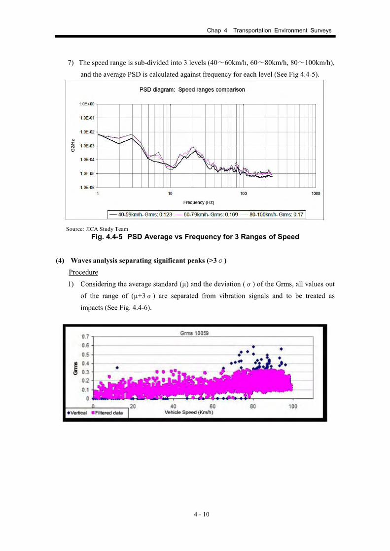
7) The speed range is sub-divided into 3 levels (40~60km/h, 60~80km/h, 80~100km/h), and the average PSD is calculated against frequency for each level (See Fig 4.4-5).
Source: JICA Study Team
Fig. 4.4-5 PSD Average vs Frequency for 3 Ranges of Speed
(4) Waves analysis separating significant peaks (>3σ) Procedure 1) Considering the average standard (µ) and the deviation (σ) of the Grms, all values out
of the range of (µ+3σ) are separated from vibration signals and to be treated as impacts (See Fig. 4.4-6).

Chap 4 Transportation Environment Surveys
4 - 11
Source: JICA Study Team
Fig. 4.4-6 Grms Values Discarding Extreme Events 2) The separated data are analyzed. The wave forms of each point are studied, analyzing
if they are isolated cases or repetitive cases within a route segment. The characteristics of each wave are observed. (See Fig. 4.4-7)
Source: JICA Study Team Fig. 4.4-7 PSD peaks vs frequency for two Grms values
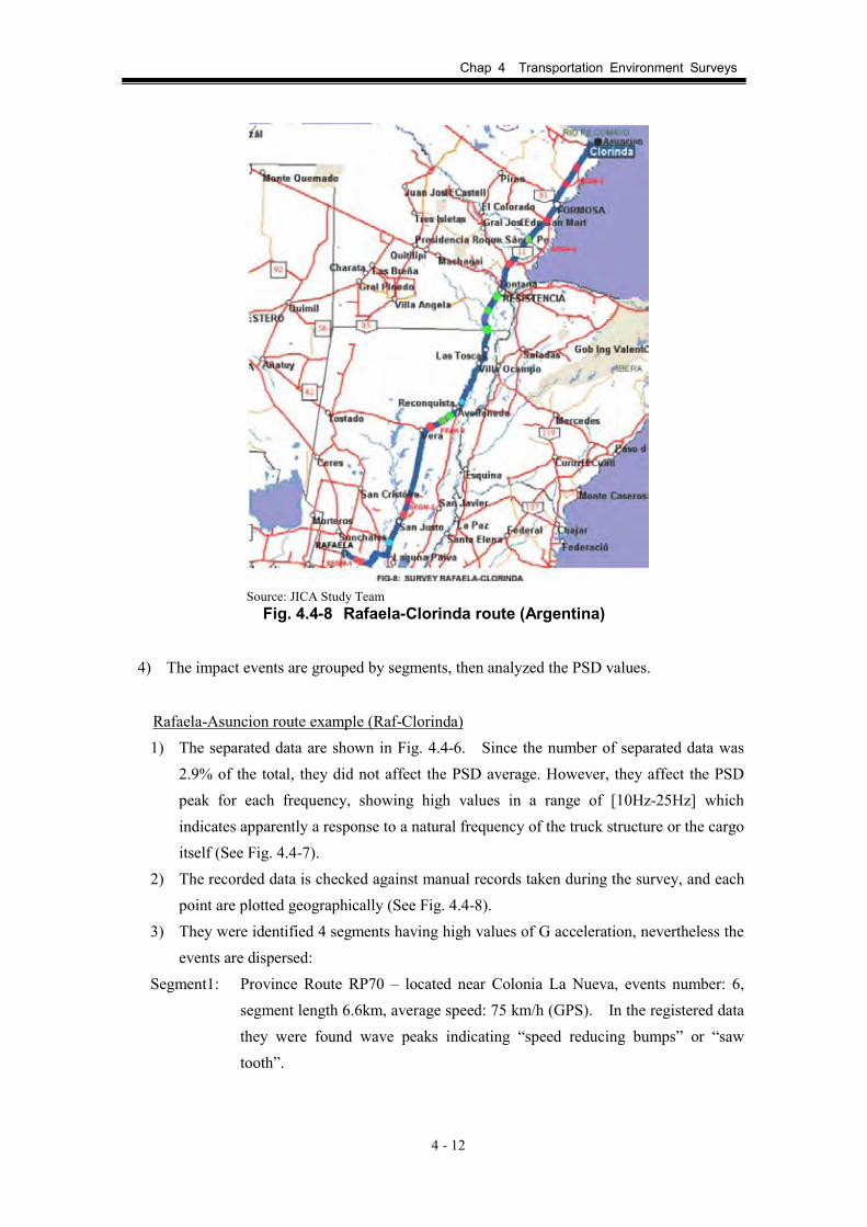
3) Map plotting of the events
For plotting of events into a map, the following color codes are applied (Fig. 4.4-8). - Spot events, segment limits: RED, - Steps on bridge edge: GREEN, - Overpass of other vehicles and others spots: BLUE.
Chap 4 Transportation Environment Surveys
4 - 12
Source: JICA Study Team
Fig. 4.4-8 Rafaela-Clorinda route (Argentina)
4) The impact events are grouped by segments, then analyzed the PSD values.
Rafaela-Asuncion route example (Raf-Clorinda) 1) The separated data are shown in Fig. 4.4-6. Since the number of separated data was
2.9% of the total, they did not affect the PSD average. However, they affect the PSD peak for each frequency, showing high values in a range of [10Hz-25Hz] which indicates apparently a response to a natural frequency of the truck structure or the cargo itself (See Fig. 4.4-7).
2) The recorded data is checked against manual records taken during the survey, and each point are plotted geographically (See Fig. 4.4-8).
3) They were identified 4 segments having high values of G acceleration, nevertheless the events are dispersed:
Segment1: Province Route RP70 – located near Colonia La Nueva, events number: 6, segment length 6.6km, average speed: 75 km/h (GPS). In the registered data they were found wave peaks indicating “speed reducing bumps” or “saw tooth”.

Chap 4 Transportation Environment Surveys
4 - 13
Segment 2: National Route RN11-San Justo city, events number:4, segment length 29km, average speed: 79 km/h (GPS), paving: repaired, route status: medium.
Segment 3: National Route RN11- Resistencia City-, events number:14; 95km, average speed: 73 km/h, “Eva Perón” port is bridge area and having slope.
Segment 4: National Route RN11–Mercedes River-, events number: 5, segment length 36.8km, average speed 79 km/h, surface: irregular, bridges and holes in the route.
4) The PSD curves were plotted: Segment 1, 2 in Fig 4.4-9 and Segment 3, 4 in Fig. 4.4-10. The Fig. 4.4-9 indicates “speed reducing bumps” and “saw tooth”, and the Fig. 4.4-10 is a segment having bridges. In both cases, the peaks are in frequencies of [2Hz , 4hz] and [15Hz], [30Hz].
Source: JICA Study Team Fig. 4.4-9 PSD average and peak vs frequency for Segment 1 and 2.

Chap 4 Transportation Environment Surveys
4 - 14
Source: JICA Study Team
Fig. 4.4-10 PSD average and peak vs frequency for Segment 3 and 4.
(5) Site observations Speed: From the data analysis, it is possible to infer that the route is suitable for running at high
speed during long spans (See Fig. 4.4-3). According to the survey, the 75% of the route was run at speed between 80 km/h and 100km/h. The PSD graphic suffer modifications and the Grms value is increasing along the increasing of speed.
Peak waves analysis, having extremely significant jumps (> 3σ): From the total of data collected, this category covers the 2.9 % of the total. This percentage does not affect the average PSD value, but it affects the peak value of PSD
(curve composed by all the peaks for each frequency), having a remarkable peak on the range of [10Hz-25Hz].
According to the analysis, they were identified 4 segments with a variety of numbers of events and having high accelerations G and dispersedly distributed.
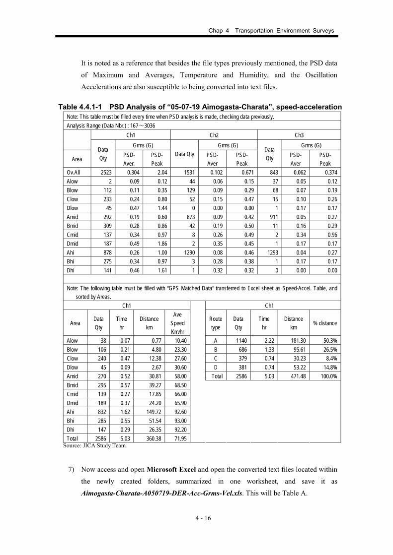
(6) DER Correction Software; Sample Analysis using GPSMap for JPI The preliminary condition is to have GPSMap for JPI installed. This software will be used to analyze the data Aimogasta-Charata-A050719-DER-10059 contained in the database. 1) First of all, the Table 4.4.1-1 needs to be prepared using Microsoft Excel. From here on
out, whenever the necessary data appears, insert them into the appropriate column.

Chap 4 Transportation Environment Surveys
4 - 15
2) Then, initiate the program to run the vibration analysis and will maintain opened the
analyzed file, 19-07-05-Aimogasta-Charata-10059.DRS. This will prompt open the Table of Acceleration Grade. Besides the DRS file, there will also be files with extension .ppv, .Svd, .THM. It will also contain the DATA.DAT file, as raw data. Not withstanding, it will include the PSD Total.Svd file.
The text files ---itp, ---.ptr, ---.utu will be located here as well. If they are not there, these can be elaborated through a text conversion that will be presented below. It must be noted, itp are title/headers, ptr are Grms, and utu are acceleration grade values.
3) The corresponding GPS data are within the 19-07-05-Aimogasta-Iguazu-PGS as Aimogasta-Charata-A050719-sn-16-HVS.cnt. These data is then matched using the
GPSMap-JPI, which will present the Table of Acceleration Grades with the velocity data. Here, click on the Text button and leave a prepared text file of the Table of Acceleration Grades. This will create a new file with the extension ---.Txt.
The above described steps reflect the preparation process.
4) First, using the current vibration analysis program, open the Table of Acceleration Grade choosing the conditions (preferences) in which the most amounts of data is available, and proceed to the PSD analysis. As a result, the Grms of the entire analyzed object’s data is created. To do this, one must first exclude the unnecessary portions of the data.
5) These results will be saved as text files. To do this, one must click and choose the option icon that appears on the top of the
screen. This will access a pull-down menu, from where one can select the option to convert to text format. At this moment, a measurement unit icon will be presented for confirmation; make sure that the acceleration grade is measured in G units.
Once the text conversion is selected, the titles that can be converted will be presented, then choose the option of Acceleration Grade and Grms, and select outputs as data. The output location can be deliberately chosen, but most commonly, these are placed in folders (directories) containing DRS files.
6) Once the processing is complete, one must confirm that the files identifiable as ---.itp, ---.ptr, ---.utu were created within the assigned output folders.
Chap 4 Transportation Environment Surveys
4 - 16
It is noted as a reference that besides the file types previously mentioned, the PSD data of Maximum and Averages, Temperature and Humidity, and the Oscillation Accelerations are also susceptible to being converted into text files.
Table 4.4.1-1 PSD Analysis of “05-07-19 Aimogasta-Charata”, speed-acceleration
Note: This table must be filled every time when PSD analysis is made, checking data previously. Analysis Range (Data Nbr.) : 167~3036
Ch1 Ch2 Ch3
Grms (G) Grms (G) Grms (G)
Area Data Qty PSD-
Aver. PSD- Peak
Data Qty PSD- Aver
PSD- Peak
Data Qty PSD-
Aver PSD- Peak
Ov.All 2523 0.304 2.04 1531 0.102 0.671 843 0.062 0.374Alow 2 0.09 0.12 44 0.06 0.15 37 0.05 0.12 Blow 112 0.11 0.35 129 0.09 0.29 68 0.07 0.19 Clow 233 0.24 0.80 52 0.15 0.47 15 0.10 0.26 Dlow 45 0.47 1.44 0 0.00 0.00 1 0.17 0.17 Amid 292 0.19 0.60 873 0.09 0.42 911 0.05 0.27 Bmid 309 0.28 0.86 42 0.19 0.50 11 0.16 0.29 Cmid 137 0.34 0.97 8 0.26 0.49 2 0.34 0.96 Dmid 187 0.49 1.86 2 0.35 0.45 1 0.17 0.17 Ahi 878 0.26 1.00 1290 0.08 0.46 1293 0.04 0.27 Bhi 275 0.34 0.97 3 0.28 0.38 1 0.17 0.17 Dhi 141 0.46 1.61 1 0.32 0.32 0 0.00 0.00
Note: The following table must be filled with “GPS Matched Data” transferred to Excel sheet as Speed-Accel. Table, and sorted by Areas.
Ch1 Ch1
Area Data Qty
Time hr
Distance km
Ave Speed Km/hr
Route type
Data Qty
Time hr
Distance km
% distance
Alow 38 0.07 0.77 10.40 A 1140 2.22 181.30 50.3%Blow 106 0.21 4.80 23.30 B 686 1.33 95.61 26.5%Clow 240 0.47 12.38 27.60 C 379 0.74 30.23 8.4%Dlow 45 0.09 2.67 30.60 D 381 0.74 53.22 14.8%Amid 270 0.52 30.81 58.00 Total 2586 5.03 471.48 100.0%Bmid 295 0.57 39.27 68.50 Cmid 139 0.27 17.85 66.00 Dmid 189 0.37 24.20 65.90 Ahi 832 1.62 149.72 92.60 Bhi 285 0.55 51.54 93.00 Dhi 147 0.29 26.35 92.20 Total 2586 5.03 360.38 71.95
Source: JICA Study Team
7) Now access and open Microsoft Excel and open the converted text files located within the newly created folders, summarized in one worksheet, and save it as
Aimogasta-Charata-A050719-DER-Acc-Grms-Vel.xls. This will be Table A.

Chap 4 Transportation Environment Surveys
4 - 17
This file will contain the information regarding the Row Number, Time and Date, Acceleration Rates in three directions and Grms, Velocity, and Location based on GPS.
Now, the measuring units of the Acceleration Rate and Grms need to be confirmed. If the units are in m/sec2, divide the values by 9.8 m/sec2, which is the Acceleration
Rate of the Gravity, and convert the measuring unit to G. As it will be necessary later, the correlation between the absolute values of the
acceleration rates and the Grms need to be determined, and should be placed on the column adjacent to the one containing the acceleration rates.
Table 4.4.1-2 Reference values by area, based on vibrations and according to
speed and route type (for plain route) Grms (G)
Acceleration (G)
Grms (m/sec2)
Acceleration (m/sec2) Area
Speed Range
Min(<) Max(≦) Min(<) Max(≦) Min(<) Max(≦) Min(<) Max(≦) Alow 0.00 0.06 0.00 0.22 0.0 0.6 0.0 2.2 Blow 0.06 0.12 0.22 0.43 0.6 1.2 2.2 4.3 Clow 0.12 0.33 0.43 1.20 1.2 3.3 4.3 12.0 Dlow
0< Vel ≦40 km/hr 0.33 - 1.20 - 3.3 - 12.0 -
Amed 0.00 0.19 0.00 0.69 0.0 1.9 0.0 6.9 Bmed 0.19 0.265 0.69 0.96 1.9 2.65 6.9 9.6 Cmed 0.265 0.33 0.96 1.20 2.65 3.3 9.6 12.0 Dmed
40< Vel ≦80 km/hr 0.33 - 1.20 - 3.3 - 12.0 -
Ahi 0.00 0.265 0.00 0.96 0.0 2.65 0.0 9.6 Bhi 0.265 0.33 0.96 1.20 2.65 3.3 9.6 12.0 Chi - - - - - - - - Dhi
80< Vel km/hr 0.33 - 1.20 - 3.3 - 12.0 -
Note: The relationship between acceleration and Grms is as follows: Acc=3.6241×Grms Source: JICA Study Team
8) After this, the PSD Analysis needs to be run based on Table 4.4.1-2, which is done by
returning to the Acceleration Rates with Velocities Table (Acc. Table) and pressing the
Auto button.
9) Subsequently, the data selection screen will be displayed. Proceed by making the necessary selections.
1. First, input the conditions for Alow
• In Adoption Level, select the Acc. to 0.0m/s2 and 0.
• In Analysis interval appointment select Entire interval appointment, and choose
Analysis start Num and Analysis end Num coinciding with the range selected in 3) above.
• Select Speed Specifications and insert the velocity range for Alow based on Table 4.4.1-2.

Chap 4 Transportation Environment Surveys
4 - 18
• Similarly, select Acc Specification and establish the range for the acceleration rate based on Table 4.4.1-2. Close attention must be paid to the measuring units and choose the corresponding one.
• Once the setups are complete, press the Execute button and process the selected data.
• When the processing is complete, return to the Acceleration Table. Here, one must confirm that the appropriate selection was processed, simply by scrolling up and down observing the worksheet.
• To save these conditions, click the Save button. Insert the name for the file where the data will be stored. To do this, a new folder for Alow needs to be created and used to save file as Alow.Svd.
2. PSD Analysis for Alow
• To do this, one must return to the DER-SMART vibration analysis program, and open the file 19-07-05-Aimogasta-Charata-10059.DRS.
• Open the list of Acceleration Rates on the screen, press the open button, and in the select file window, select the Alow.Svd that was saved during step 1 in part 9) and press the save button.
• In the next screen, press the Initiate (Start) button.
• At this point, the data will be set based on the selection conditions of Alow. Press the PSD analysis button. The calculation process for the PSD will be performed in waves, and the measuring unit will be in G2/Hz. Press the OK button to begin the analysis.
• Once the results from the analysis are displayed, confirm the number of data, Grms, etc., and if no problems can be detected, press the options button once the necessary data was copied into Table 4.4.1-1, and proceed to converting all the items except for the oscillations of the acceleration rates into text.
• Create a new Alow folder and save the files there. An Alow.itp file will be created.
• Open this file using Excel. If all files are selected to be displayed, there will be other files besides the Alow.itp, including Alow.otd, Alow.ptp, Alow.ptr and Alow.utu. As previously mentioned, the .itp are title and headers, ptr are Grms, .utu are acceleration rates, .otd are temperature and humidity, and .ptp are PSD.
• This is the last step for the Alow vibration software analysis.
• Therefore, to return to the GPSMAP for JPI, open the Acceleration Table. In other words, return to step 7).
• To perform the Blow analysis, repeat this process from step 8). 3. The storing of all the text files need to be completed, including all the PSD files up to
Dhigh. From here on forward, all the processing and editing will be performed in
Excel, and therefore all other windows and running programs can be closed.

Chap 4 Transportation Environment Surveys
4 - 19
10) Roadway Type, Data Quantity based on the Classification of Circulation Velocities, Traveled Distance, Traveling Time, PSD. 1. Finish the Excel worksheet 4.4.1-1. The number of data values, maximum and average
PSD can be inserted after each PSD analysis for the different classes are displayed.
2. Perform the analysis solely in the Ch 1 (vertical) direction; the other directions will be
performed depending on necessity.
3. Confirm the measuring intervals based on the time data. The current study has an
established measuring interval of 7 seconds, and therefore the actual travel time can
be obtained by multiplying the number of data by 7 (seconds).
4. To determine the traveling distance for each class, a new table needs to be created by
copying the data from Table A. This table will be named “Worksheet based on
Velocity – Grms.” All the unnecessary data will be eliminated in the new table. The
data to be deleted consists of that recorded before the start of the actual measurement,
and the data between Num1-166 and Num3037-10000 where there was no variation
in the velocity set at 50km/hr because no GPS data was available.
5. Change the order of the columns so that the absolute values of the acceleration rates
Ch1 are next to the Speeds.
6. Next to the Speed column, place the formula to calculate the traveled distance by
multiplying velocity by 7 seconds=0.001944hr, so that with every velocity, a traveled
distance can be calculated.
7. Then, rearrange the table values based on the Speeds data. Based on the reorganized
table, classify the velocities in zones of low, medium and high velocities. It is
convenient to leave three empty colored rows.
8. Rearrange the values under the low velocity zone based on the acceleration rate, and
classify the zones A, B, C, D, in conformity with Table 4.4.1-2. Insert 3 blank rows
with distinctive colors for each zone.
9. Repeat the previous step for the zones of medium and high velocities.
10. Use the blank separation rows to insert the summarized data for each zone, which
include average velocity and traveled distance in each zone. Insert these resulting
values into Table 4.4.1-1. These values will be similar to those obtained during the
PSD analysis. There can be variations between the data, but there should be no major
differences.
With the information gathered, Table 4.4.1-1 can be filled, and the composition ratio
based on roadway types can now be calculated.

Chap 4 Transportation Environment Surveys
4 - 20
11) Processing PSD waves in each zone. 1. The PSD waves for each zone will now be summarized and the testing parameters will
be determined.
2. First, the PSD data which is saved as a text file is summarized into one Excel file. At
this point, create a file named “PSD by Zones.”
3. Open the ---.ptp files created in step 9) using Excel, orderly from Alow to Dhigh.
Copy these files in the “PSD by Zones.”
4. Use the first worksheet as the general page, and starting on the second worksheet, past
the data regarding each zone in all three directions, one sheet per each zone. Identify
each created sheet by inserting the name of each zone within the header of each page.
5. Once all the data is copied and pasted, copy the data for the upward and downward
directions and those on the Frequency column. Order them by frequency and paste
them on the first page (general worksheet). Before, the first worksheet needs to be
renamed “General Worksheet Ch1.”
6. Once the copy/paste is completed, rearrange the appropriate columns and the
following PSD curves will be created.
a. Four (4) linear PSD graphs summarized by roadway, A (low, medium, high), B (low,
medium, high), C (low, medium), and D (low, medium).
b. Three (3) linear PSD graphs summarized by velocity sections, Low (A, B, C, D),
Medium (A, B, C, D), and High (A, B, D).
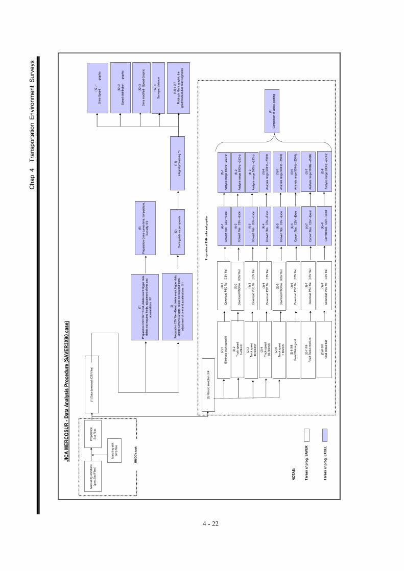
4.4.2 Data Analysis Procedure for SAVER3X90 Sensors
For data analysis process of collected data during the Transportation Environment Surveys,
by using SAVER3X90 sensors, it is explained on next pages the procedure according to JICA
MERCOSUR process.

Cha
p 4
Tra
nspo
rtatio
n En
viro
nmen
t Su
rvey
s
4 - 21
JICA
MER
COSU
R - D
ata
Anal
ysis
Pro
cedu
re (S
AVER
3X90
cas
e)
The
follo
win
g is
the
proc
edur
e fo
r Dat
a An
alys
is o
f vib
ratio
ns re
cord
ed d
urin
g th
e Tr
ansp
orta
tion
Envi
ronm
ent S
urve
y by
usi
ngth
e SA
VER
sens
ors.
1) A
pplie
d te
rmin
olog
y S
xd fi
les
"Rau
gh D
ata"
file
s, re
cord
ed b
y th
e SA
VER
sens
ors.
Sxe
files
Mod
ified
dat
a fil
es fr
om S
xd d
ata
by S
AVER
's p
rogr
am, u
nder
MS
Acce
ss fo
rmat
.
GPS
file
sG
PS d
ata
reco
rded
by
GPS
sys
tem
, ind
icat
ing
the
truck
pos
ition
, tim
e.
2) D
ata
Anal
ysis
wor
ks fl
ow d
iagr
am
For i
ssui
ng th
e re
ques
t of D
ata
Anal
ysis
to K
obe
Univ
ersi
ty, b
asic
ally
a S
xe fi
le is
tran
sfer
red,
in w
hich
they
are
incl
uded
th
e po
sitio
ning
dat
a af
ter c
ompl
ete
the
data
mat
chin
g of
vib
ratio
n da
ta w
ith G
PS d
ata.
Rega
rdin
g to
the
data
ana
lysi
s w
orks
, the
y ar
e di
vide
d in
to 2
mai
n ac
tiviti
es.
a) W
orks
by
usin
g SA
VER
prog
ram
s (m
ainl
y to
obt
ain
PSD
data
) and
exp
ort t
o an
EXC
EL fi
le.
b) D
ata
Anal
ysis
wor
ks b
y us
ing
EXCE
L fu
nctio
ns.
Cha
p 4
Tra
nspo
rtatio
n En
viro
nmen
t Su
rvey
s
4 - 22
JICA
MER
COSU
R - D
ata
Anal
ysis
Pro
cedu
re (S
AVER
3X90
cas
e)
NOTA
S:
Tare
as c
/ pro
g. S
AVER
Tare
as c
/ pro
g. E
XCEL
Mea
surin
g vib
ratio
ns(
prep
.Sxd
File
s)
(2)-1
Elim
inat
e tru
ck s
peed
0
(2) R
ecor
d se
lect
ion ※
4
(1) D
ata
down
load
(CSV
file
s)Pr
epar
atio
nSx
e Fi
les
Mat
chin
g wi
thG
PS fi
les
(2)-2
Truc
k sp
eed
0-40
km/h
(2)-3
Truc
k sp
eed
40-6
0km
/h
(2)-4
Truc
k sp
eed
60-8
0km
/h
(2)-5
Truc
k sp
eed
> 80
km/h
(3)-1
Down
load
PSD
file
(CS
V fil
e)
(3)-2
Down
load
PSD
file
(C
SV fi
le)
(3)-3
Down
load
PSD
file
(CS
V fil
e)
(3)-4
Down
load
PSD
file
(CS
V fil
e)
(3)-5
Down
load
PSD
file
(C
SV fi
le)
(5)-1
Anal
ysis
rang
e 50
0Hz→
250H
z
(5)-2
Anal
ysis
rang
e 50
0Hz→
250H
z
(5)-3
Anal
ysis
rang
e 50
0Hz→
250H
z
(5)-4
Anal
ysis
rang
e 50
0Hz→
250H
z
(5)-5
Anal
ysis
rang
e 50
0Hz→
250H
z
(6)
Com
plet
ion
of ta
bles
, plo
tting
(10)
Sorti
ng d
ata
as p
er s
peed
s(1
1)In
tegr
al p
roce
ssin
g *3
(12)
-1G
rms-
Spee
d
gra
phic
UNIC
O's
task
Prep
arat
ion
of P
SD ta
bles
and
gra
phics
(4)-1
Conv
ert f
iles
CSV
→Ex
cel
(4)-2
Conv
ert f
iles
CSV
→Ex
cel
(4)-3
Conv
ert f
iles
CSV
→Ex
cel
(4)-4
Con
vert
files
CSV
→Ex
cel
(4)-5
Con
vert
files
CSV
→Ex
cel
(2)-6
※6
Road
Sta
tus:
good
(2)-7
※6
Roa
d St
atus
:med
ium
(2)-8
※6
Road
Sta
tus:
bad
(3)-6
Down
load
PSD
file
(CS
V fil
e)(5
)-6An
alys
is ra
nge
500H
z→25
0Hz
(4)-6
Conv
ert f
iles
CSV
→Ex
cel
(3)-7
Down
load
PSD
file
(C
SV fi
le)
(5)-7
Anal
ysis
rang
e 50
0Hz→
250H
z(4
)-7C
onve
rt file
s C
SV→
Exce
l
(3)-8
Down
load
PSD
file
(CS
V fil
e)(5
)-8An
alys
is ra
nge
500H
z→25
0Hz
(4)--
8Co
nver
t file
s C
SV→
Exce
l
(12)
-2Sp
eed
dist
ribut
ion
g
raph
ic
(12)
-3G
rms
mod
ified
- Sp
eed
Gra
phic
(12)
-4Su
rvey
ed d
ista
nce
(7)
Prep
arat
ion
CSV
file→
Exce
l, de
lete
eve
nt tr
igge
r dat
a,de
lete
not
requ
ired
field
s, a
djus
tmen
t of t
ime
and
acce
lera
tions
※1
(8)
Prep
arat
ion
Grm
s cu
rves
-tim
e, te
mpe
ratu
re,
hum
idity
※2
(9)
Prep
arat
ion
CSV
file→
Exce
l, de
lete
eve
nt tr
igge
r dat
a,de
lete
Grm
s<0,
02 d
ata,
del
ete
not r
equi
red
field
s,ad
just
men
t of t
ime
and
acce
lera
tions
※1
(12)
-5 ※
7Pl
ottin
g in
Grm
s gr
aphi
c th
ego
od/m
ediu
m/b
ad ro
ad s
egm
ents

Cha
p 4
Tra
nspo
rtatio
n En
viro
nmen
t Su
rvey
s
4 - 23
JICA
MER
COSU
R -
Data
Ana
lysi
s Pr
oced
ure
( SA
VER3
X90
sens
or c
ase)
NOTE
S:
※1:
※2:
※3:
※4:
※5:
※6:
※7:
In th
e ca
se o
f sam
plin
g tim
e of
1m
s, th
e SA
VER
prog
ram
cal
cula
tes
auto
mat
ical
ly th
e PS
D va
lues
with
in a
rang
e up
to 5
00Hz
. In
this
cas
e, it
is re
quire
d to
mak
e a
re-c
alcu
latio
n of
PSD
with
in a
rang
e up
to 2
50Hz
, in
orde
r to
mat
ch w
ith D
ER-S
MAR
T sy
stem
.
The
PSD
valu
es a
re m
anua
lly c
alcu
late
d fo
r eac
h ro
ute
cond
ition
(goo
d, m
ediu
m, b
ad),
base
d on
a p
revi
ous
sele
ctio
n of
rela
ted
rout
e se
gmen
ts a
nd re
ferr
ed to
"t
ime
reco
rds"
regi
ster
ed m
anua
lly d
urin
g th
e su
rvey
s.
Sinc
e th
e se
lect
ion
of ro
ute
segm
ents
is m
ade
man
ually
, thi
s pr
oces
s re
quire
s tim
e.
For
this
reas
on, t
his
proc
ess
will
be
deve
lope
d on
ly fo
r the
rout
e of
Bra
sil (
Bele
m-S
an P
ablo
, Sep
21-2
2) ;
Join
ville
-San
tiago
rout
e an
d Ca
mpi
nas-
Reci
fe ro
ute.
The
plot
ting
proc
ess
for i
dent
ify th
e ro
ute
stat
us o
f "go
od",
"med
ium
" and
"bad
", is
mad
e m
anua
lly, s
o th
at it
requ
ires
time.
The
dat
a to
be
proc
esse
d m
anua
lly
are
thos
e in
dica
ted
in ※
6.
At th
e st
age
of "e
xpor
ting"
dat
a fro
m S
AVER
's p
rogr
am to
an
EXCE
L fil
e, th
e tim
e is
indi
cate
d by
GM
T an
d th
e sp
eeds
by
mile
s/ho
ur.
The
se d
ata
mus
t be
conv
erte
d in
to "l
ocal
tim
e" a
nd "k
m/h
".
See
plea
se E
XCEL
sam
ple
file.
See
plea
se E
XCEL
sam
ple
file.
The
SAVE
R pr
ogra
m is
sui
tabl
e fo
r a fa
st s
elec
tion
of d
ata,
bas
ed o
n re
quire
d sp
eed
valu
es.
H
owev
er, f
or th
e de
letio
n of
zer
o sp
eed
data
, it i
s ca
rrie
d ou
t bu
Grm
s <
0.02
con
ditio
n.
So
urce
: JIC
A S
tudy
Tea
m

Chap 4 Transportation Environment Surveys
4 - 24
4.4.3 General Aspects of the Transportation Environment and the Measuring Data
The data that was summarized with the aim to define standard reference values to evaluate the packaging tests. The following is a summary of the observed characteristics.
(1) Differences on road transportation between Japan and MERCOSUR There still are many damage accidents even though the JIS standards are satisfied. The
situation of MERCOSUR is compared with Japanese case as below.
1) Different Vehicle Type Firstly, from a visual comparison perspective, approximately 80% of the freight
transportation means utilized in the MERCOSUR region consist of trailers, whereas it is estimated that in Japan, slightly over 80% of the distribution is done with trucks.
A certain Japanese company tried changing their trucks by trailers, which allow a larger volume of freight transfer per trip, to improve the transportation efficiency, but this lead to an increased number of damaged goods. A study was conducted to determine the causes, and it was discovered that there was a high difference in the emitted vibrations between the two means. At that time, the problem was resolved by changing the suspension types on the trailers, adopting an air suspension.
The vehicular inspection system in Japan is such that it incurs high maintenance costs to older vehicle models to satisfy the regulations in place. On the other hand, newer vehicle models abiding by the low gas emission regulations enjoy tax exemption advantages.
During the execution of the transportation tests, performed under the scope of the project at hand for the JICA development study, there were situations that arose impeding the gathering of data due to breakdowns and repairs on the vehicles utilized for the testing.
2) Freight’s (Cargo’s) Conditions
From what was observed, with the exception of large freight such as those with electrical household appliances, the small and medium ones, which represent the majority of the transported freight volume, were placed on pallets and set in place with elastic film to avoid their displacement and disarrangement. The handling during the loading and unloading of the freight is primarily done with forklift trucks.
The dimensions of the pallets employed by the companies that participated in this study correlate to the size of the loading bed of the trailers and have practically no unoccupied space. Maybe due to this geometry, the van type transports do not require stabilizers to

Chap 4 Transportation Environment Surveys
4 - 25
avoid the disarrangement of the cargo. When loading refrigerators onto the loading bed, these are tied with ropes and covered with cloths.
Even in Japan, there has been an increase in the use of pallets to reduce the cargo loading and unloading time, but the trends are still low. The system of cargo transfer on pallets provides stability to avoid disarrangement and improve the loading ratio, although it has its disadvantages when it comes to impacts during their handling.
The loading ratio for those products of high specific weight, such as foods, is almost at the maximum levels, leaving minimal space on the upper parts of the transport. The products with low specific weights, such as refrigerators, are loaded to the maximum volume capacity, but it is estimated that their specific weight does not reach 60%. This is similar to Japan.
In general, the lower the loading ratio, the higher the vibrations felt on the loading bed.
3) Traveling Distance and Transportation Conditions (Circulation) In Japan, the distance between the large consumptions centers such as Tokyo, Nagoya
and Osaka is between 600km to 700km, and therefore most of the time, the transportation distance for each trip is less than 1,000km. Even the longest trips are considered to be around 2,000km, whereas in the MERCOSUR, the international transportation distance can be greater than 3,000km. In Argentina and Brazil, even some domestic trips exceed 3,000km in distance.
Given this situation, most of the traveling is done on highways for long periods of time, and therefore the majority of the recorded average speeds surpass 80km/hr. Given that the kinetic energy of the entire transport increases proportionally to the velocity squared (v2), given constant conditions to the roadway, the vibration produced on the transport’s loading bed also increases proportionally to the vehicle’s velocity. From this, it can be assumed that the vibration levels in the MERCOSUR are greater than those experienced in Japan.
Nevertheless, the transported distances is equal to those conducted in the United States or Europe, and therefore the causes that produces higher stress levels than those contemplated in the ISO and ASTM testing norms must be determined.
4) Driver’s Skill and personal character
In practically, all trips performed as part of this study, there has been an assigned chasing vehicle with members from the study team to make observations of both the roadway conditions as well as the traveling itself. All vehicles were carefully operated by expert drivers, all excellent people and proud of their profession. Certainly, there are registries of driving speeds exceeding the ones verified during a normal trip once the participants took separate directions, and the drivers went to spend the night in the trucks in the parking lot,

Chap 4 Transportation Environment Surveys
4 - 26
and the remaining of the team spent the nights at hotels; but it should be noted that there has also been parts where the truck and the chasing car had to travel in very low speed, forming a single file.
Based on the collected data regarding the relation between the traveling velocity and the magnitude of the generated vibrations, it is observed that there are various sections of the trip where the traveling velocity surpasses 100km/hr, but the levels of vibrations are significantly lower compared to other sections traveled at lower velocities. It can be assumed that the drivers will travel at high velocities only in sections where the roadway conditions present a certain level of security to allow the higher speeds without causing major impacts or vibrations.
5) Roadway Surface Conditions and Curves
Currently in Japan, with the exception of mountainous regions without human settlements, practically all roads are regularly maintained and repaired, and there are no roads with poor surface conditions.
In the MERCOSUR region, probably due to its extensive territory, there are large sections of roadway where the maintenance work is not reached, and when traveling these sections, the vehicle produces high levels of vibrations.
Even so, it is considered that the maximum level of vibration produced during roadway transportation in Japan is comparable to those observed in the MERCOSUR. The problem consists on the frequency in which these high vibrations are observed.
If the same trailer were to be utilized in Japan and the MERCOSUR, the maximum observed vibration levels will be the same in both, but it is estimated that the number of occurrences of such maximum values will be very different.
The main reason causing these differences are the roadway’s surface conditions and the traveling velocities.
The curves of the roadway also affect the traveling velocity. In Japan’s case, the traveling velocities are obviously limited to the roadways with short tangent sections and their high number of continuous curves.
On the other hand, given the vast territory of the MERCOSUR region, its roadways have straight tangents for hundreds of kilometers, incomparable to the tangent sections that may be found in Japan. As such, and with the low traffic volumes, there is a satisfactory situation to travel at high velocities. Even with the poor roadway surface conditions, if the wheel is in safe hands, it seems that high velocity travel can be done without problems.
Chap 4 Transportation Environment Surveys
4 - 27
4.5 Damages on Target Products and Damage Index
Damages on target products and packaging have been studied on transported cargoes from Brazil to Chile, during the Transportation Environment Survey. They were home refrigerators (capacity: 310L, truck loading capacity: 142 units). The route stretch and conditions have been indicated in the study content described above, so that on this section it is described the results of the cargo visual inspection on the arrival warehouse at Chile side.
(1) Product Inspection: Since the packaging was not allowed to be opened, the full evaluation could not be done.
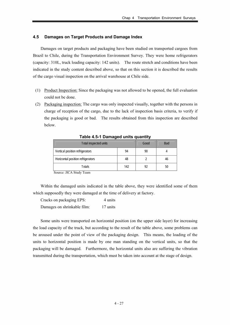
(2) Packaging inspection: The cargo was only inspected visually, together with the persons in charge of reception of the cargo, due to the lack of inspection basis criteria, to verify if the packaging is good or bad. The results obtained from this inspection are described below.
Table 4.5-1 Damaged units quantity
Total inspected units Good Bad
Vertical position refrigerators 94 90 4
Horizontal position refrigerators 48 2 46
Totals 142 92 50 Source: JICA Study Team
Within the damaged units indicated in the table above, they were identified some of them
which supposedly they were damaged at the time of delivery at factory. Cracks on packaging EPS: 4 units Damages on shrinkable film: 17 units Some units were transported on horizontal position (on the upper side layer) for increasing
the load capacity of the truck, but according to the result of the table above, some problems can be aroused under the point of view of the packaging design. This means, the loading of the units to horizontal position is made by one man standing on the vertical units, so that the packaging will be damaged. Furthermore, the horizontal units also are suffering the vibration transmitted during the transportation, which must be taken into account at the stage of design.

Chap 4 Transportation Environment Surveys
4 - 28
Corner support moved at the back side of truck. EPS edges are slightly damaged.
Horizontal position units loading. Cargo and personnel under dangerous procedures.
Cargo moved during transportation. EPS slightly deformed due to cargo displacement for 8cm.
Shrinkable film meltdown. Film touching a portion of refrigerator.
Source: JICA Study Team Fig. 4.5-1 Cargo arrived at destination and damages observed
4.5.1 Status of Damages of Packaging
For the analysis of the damages of packaging based on collected information during this Study, it was observed some difficulties as follows:
(1) The information is coming from several sources, but there are no systematic data gathering for statistical analysis.
(2) In case of products to be sold commercially, it is not possible to carry out an exhaustive study since it is not possible to open the packaging one by one.
(3) The information can not be published, due to commercial confidentiality rules, even working with cooperating companies.
Chap 4 Transportation Environment Surveys
4 - 29
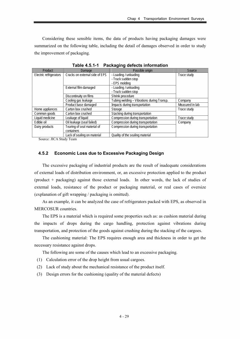
Considering these sensible items, the data of products having packaging damages were summarized on the following table, including the detail of damages observed in order to study the improvement of packaging.
Table 4.5.1-1 Packaging defects information
Product Damage Possible origin Source Cracks on external side of EPS - Loading / unloading
- Truck sudden stop - EPS molding
External film damaged - Loading / unloading - Truck sudden stop
Discontinuity on films Shrink procedure
Trace study
Cooling gas leakage Tubing welding – Vibrations during Transp. Company
Electric refrigerators
Product base damaged Impacts during transportation Measured in lab Home appliances Carton box crushed Storage Common goods Carton box crushed Stacking during transportation
Trace study
Liquid medicine Leakage of liquid Compression during transportation Trace study Edible oil Oil leakage (seal failed) Compression during transportation
Tearing of seal material of containers
Compression during transportation Dairy products
Lack of sealing on material Quality of the sealing material
Company
Source: JICA Study Team
4.5.2 Economic Loss due to Excessive Packaging Design
The excessive packaging of industrial products are the result of inadequate considerations of external loads of distribution environment, or, an excessive protection applied to the product (product + packaging) against those external loads. In other words, the lack of studies of external loads, resistance of the product or packaging material, or real cases of oversize (explanation of gift wrapping / packaging is omitted).
As an example, it can be analyzed the case of refrigerators packed with EPS, as observed in MERCOSUR countries.
The EPS is a material which is required some properties such as: as cushion material during the impacts of drops during the cargo handling, protection against vibrations during transportation, and protection of the goods against crushing during the stacking of the cargoes.
The cushioning material: The EPS requires enough area and thickness in order to get the necessary resistance against drops.
The following are some of the causes which lead to an excessive packaging. (1) Calculation error of the drop height from usual cargoes. (2) Lack of study about the mechanical resistance of the product itself. (3) Design errors for the cushioning (quality of the material defects)

Chap 4 Transportation Environment Surveys
4 - 30
Protection against vibrations: The vibration characteristics of the packaged cargo, which is determined by the thickness
and area of EPS material – supporting and fixing the product – and the weight of the product, could be amplified during the transportation process transmitting the vibrations to the product, so that it can exceed the allowable vibration level of the product and then producing damages. In this case, the causes of excessive packaging could be centered in the following items.
(1) Lack of evaluation of vibrations, originated by the excessive thickness and area of EPS material.
(2) Lack of study of the vibration resistance of the product. (3) Calculation error of vibrations aroused during the transportation.
Crushing: The EPS must be sized (thickness and area) in such way that it can resist the weight of the
cargo during the time of storage. In this case, the cause of excessive packaging is an incomplete evaluation for EPS Creep characteristics.
As described above, due to an non adequate values of thickness and area of EPS material,
the package results on a oversized design with an increased external dimensions. Furthermore, it is added the problem of lack of precise data of the transportation
environment. As result of all of these, the cost is increased due to materials, processing, transportation up to the end of user, loading / unloading, so that even in the case that the material and processing costs are relatively low, the total distribution cost as a whole will be completely “in red”.
4.5.3 Economic Losses due to Damages on Products
As an example, on the following Table, it is shown the case of damages observed on transported goods, i.e. refrigerators, analyzed during the study of home appliances.
Table 4.5.3-1 Break down of defects on product (refrigerator)
Failure Percentage (%) Failure on door adjustment 0.46 Failure on electrical wires 0.42 Failure on door right angle 0.28 Failure on drain system 0.27 Failure on doors due to impacts 0.13 Failure on packaging 0.03 Others 0.33
Total 1.92 * The percentage is an incidence rate of defects out of 17,000 inspected units.
Source: JICA Study Team
Chap 4 Transportation Environment Surveys
4 - 31
The total 1.92% defects observed at the end of the distribution represent a high value from production point of view. Looking the details of type of defects, it can be seen that the 25% are related to the doors problems. It can be guessed that this is due to the displacement of the door originated by the impacts produced by vibrations.
From this information, it can be related to the loss of profit due to reduction of value due to replacement of parts, spending for non-charged repair works, reduction of commercial value and loss of quality of the product. It must be remarked that the author could not obtain the exact quantity of damaged products during the Study.
Regarding to the damages prevention measures, it must be analyzed the type of damages, and the system of validation of the product / packaging for the design of packaging as well.
We are sure that, all the measurements, data analysis, and determination of the Reference Guideline for Packaging Tests etc developed during this Study, will have a practical application.

CChhaapptteerr 55 DDaattaa CCoolllleeccttiioonn aanndd DDaattaa AAnnaallyyssiiss ooff TTrraannssppoorrttaattiioonn EEnnvviirroonnmmeenntt SSttuuddyy

Chap 5 Data Collection and Analysis of the Transportation Environment Study
5 - 1
Chapter 5 Data Collection and Data Analysis of Transportation Environment Study
As a part of the current JICA Study, the Demonstration Test of Transportation Environment Study was performed in February 2005 in Argentina. After that, the collected data related to the transportation conditions, intensively executed by each member country of MERCOSUR, were stored as “raw” data, following the classification method agreed between the JICA Study Team and the members of their counterpart institutions, at the time of the presentation of the Progress Report. Following this stage, the analytical work was conducted in compliance with the JICA MERCOSUR (SAVER3) analysis methodology, to establish reference values as standards to evaluate packaging through tests. This task was undertaken by the JICA Study Team and their counterparts, coordinated by INTI Argentina as the MERCOSUR Coordinator. As a result of this coordinated effort, the JICA Study Team finalized on setting the "Reference Value for Evaluation of Packaging Tests” (preliminary version).
5.1 Construction of the MERCOSUR Database
Introduction
Regarding to the construction of the MERCOSUR database, a data classification method has been issued and agreed upon at the stage of the Progress Report, at the meeting of the four (4) countries on February 16th 2006 (see Fig. 5.1-1). However, it is considered that there is the difficulty of directly taking upon the construction of this database, because of insufficient capacity of the existing counterparts’ computer systems on both hardware and software, and the lack of human resources for the task. For that reasons, it was decided to explain the general guideline in this chapter, which will be complemented in detail in the Chapter 10.
The database, containing information about collected data, result of data analysis,
numerical information and graphics (hereinafter “informative resources”) developed by the “Study of Improvement of Packaging Technology for Merchandise Distribution in MERCOSUR” integrated by Argentina, Brazil, Paraguay and Uruguay, will become an important source of information regarding improvement techniques for transporting and packaging of products within the region once it is placed on the Internet Website for public access.

Chap 5 Data Collection and Analysis of the Transportation Environment Study
5 - 2
5.1.1 Use of the Database
As the final users of the database, two main types of users have been defined, and to be considered for the construction of the database for Web site.
1) Passive users, whose main objective is the sole acquisition of information, for example,
for the study of specialized knowledge. 2) Active users, seeking information and graphics for managerial, educational or
investigative purposes that are provided to the public via the Internet Website. The use case 1) is similar to any Internet Web Page, whereas the data corresponding to 2)
will require characteristic properties of a database. In this case, the provider of the information must prepare high quality data and validate to be used as a reliable source. Also, in the use case 2), the informative resources open to the public use may be utilized as secondary sources, in other words, the information may be downloaded and used as presentational material in seminars and conferences as visual aides in form of films, posters or prints, CD-ROM, and even link to other websites. The database may be a non-profit source of information for investigative or educational purposes, or, it can be commercialized. Regardless of the case, the copyright must be properly referenced throughout its use.
5.1.2 Group of Users and Correspondence Needs
The informative resource database for the field of packaging technology can be used on several ways, and the type of users would be diversified also. The published information on the web can be accessed by a wide variety of users. These users may also issue questions, comments and requests regarding the provided information, and therefore a mean to respond to such demand must be defined.
5.1.3 Useful Database
The important thing is to “construct something that is truly useful.” A mean or vehicle is required, to transmit the information, and the user will acquire the information through the mean deemed most user-friendly. Placing the information in Web format for public access only makes sense if the provided information could not be given through the currently conventional means of communication. It is obvious that a database will not be completed before its construction is finished. In order to maintain the usefulness of a database, it is required a constant work, not only to update and correct the data, but also working to address the solicitation and comments of its users.

Chap 5 Data Collection and Analysis of the Transportation Environment Study
5 - 3
5.2 Aspects to Be Considered for the Database Development
5.2.1 Database Structure
(1) Information Administration for Non-Specialized and General Public Users The database can be accessed by the general public, therefore their structure cannot account
solely on the specialized sector. Wherever possible, the organizational design, menu and content, must be oriented for both types of users. It would be beneficial to design separate menus for those “Specialized” and “General Public” users. The important aspect is to consider the accessibility from the eyes of the users of the database.
(2) Database as a Secondary Source Anyone may access and download the information placed on the Web. To accomplish this,
the users must indefectibly obtain the authorization from the author of the work to be able to access and utilize the information.
(3) Naming and Location of the Files
While elaborating the database, close attention must be paid to the file naming criteria and their location. In general, any Website, once uploaded and opened to the public, it must be continuously updated which makes it essential to have a consistent file name and location from the conception of the database. Once placed on the Web, it is not convenient to change the location of the files because the html files are used by the Internet search engines to browse its contents, and most users will access the site through them. Changing file names and location may not only cause erroneous links, but it may also complicate the search engines browsing capabilities, therefore reducing accessibility and functionality of the Web Site.
Special attention must be paid for a database with large volume of information, such as the one at hand for packaging technologies for transportation, but this holds true for any Web Page in general. Regarding the location of the files, it is convenient to place the informative resources collected from the survey field, such as the images (maps, photographs of road conditions, etc.) and the numerical and text information, including the results of the analysis, to be stored in different directories (or folders). If a directory (or folder) contains hundreds or thousands of files, it makes their handling quite difficult. Therefore, it is convenient to have a previously agreed maximum number of files per each directory, and once that limit is reached, a new directory shall be created.

Chap 5 Data Collection and Analysis of the Transportation Environment Study
5 - 4
5.2.2 Navigators and Search Engines
(1) WWW Browser as Database Browsing Software There are some databases available through the internet which requires a particular
web-browser, but in general, most of these sites can be viewed through mainstream WWW browsers, such as Netscape, Internet Explorer, etc. It is convenient that the database published on the web will be accessible with any mainstream browser and not limited to a particular version or program.
(2) WWW Browsers, HTML Files, and Search Engines A database that can be accessed through WWW browsers means that the final output
format (layout) is controlled by the HTML (hypertext markup language) files. However, there are two types of data published on the web:
(a) The main database in controlled through a specific program, and in order to cover the
needs of each user accessing through the web, the program will automatically create a HTML file with the inquired information.
(b) All the data is located from the beginning on the server in the form of HTML files. In this case, all the files need to be connected and unified to allow the search engines to
gather the necessary information for its searches.
5.2.3 HTML File Design
(1) Avoid Potential Browsing Software Errors in Perception HTML is a simplified language based on the SGML (Standard Generalized Markup
Language) adopted as a standard by the ISO 8879. The SGML in itself an extremely complicated language, and therefore for practical reason, a simpler version known as HTML is used.
To avoid functionality issues, it is preferable to elaborate a web site using generalized HTML format, practices that have been in place and have been tested for several years, and preclude the use of newer and more complex functions that may generate confusion among the users.
(2) Needs for Metadata Looking the large number of published information on the web over the last few years,
sometimes it is complicated to obtain matching search results by an Internet even using reliable search engines. To address this issue, presently on the Internet world it is recommended to insert

Chap 5 Data Collection and Analysis of the Transportation Environment Study
5 - 5
a key-word (metadata) which allows the identification of the content within each HTML file. Metadata is defined as a data of the data, in other words, information regarding each piece of data.
5.2.4 Information Quality Maintenance on Laboratory Test and the Roadway and Transportation Conditions
The most important aspect is the level of utility of the information that will be made available to the public.
(1) Providing High Quality Images There are large numbers of pages containing images (photographs, etc.) that are placed with
the sole purpose to be displayed on the screen. These images can be amplified only to a 2x2 to 4x4 ratio. Also, the images’ resolution is low and not adequate for printing. This occurs because the printed image’s resolution is very high (greater than 600 dpi) compared to the screen’s resolution of 72 dpi. To obtain printable images, the file needs to be accommodated for at least 8x8 to 16x16 ratios to the resolution on the screen. To obtain such resolution, the photographs or image sources must be passed through a scanner and set its resolution to a setting equal to or higher than the printed source, in other words, at least 600 dpi.
(2) Image’s Objectivity If the images are going to be published on a website for general use, they must be visually
attractive. To obtain this, in most cases, even in photographs of nature, retouching may be required.
(3) Clarity and Color There are cases in which the photographs need to be altered in its appearance from the
moment the photograph is taken until the film is developed and digitized, and in some cases manipulation of the colors, as in microscopic images.
Chap 5 Data Collection and Analysis of the Transportation Environment Study
5 - 6
5.3 Elaboration through the Publication of the Database
5.3.1 Checking Grammar and Links
Once the web page is set up, an exhaustive checking process must be undertaken reviewing the content of each HTML file before they are published on the web. In other words, the precision of each link to texts and images, internal and external to the page, and as well as the logistic grammar of the HTML text need to be reviewed.
5.3.2 Correcting Search Engine’s Perception Errors
In many cases, the output layout (presentation on the screen) of the HTML files could be viewed differently, depending on the Web browser used. This aspect must be carefully considered while creating the HTML files, but these must be revised once the varying displays are checked on the different browsers and make the necessary adjustments to obtain the most homogeneous layout possible.
5.3.3 Advantages and Disadvantages of the DNS (Domain Name Server)
Reference Function
Users would logically prefer obtaining the queried information as soon as possible from the accessed web server. The website server administrator desires to acquire the location and the number of users from where the user accesses to gain a better understanding of the types of utilizations of the server. The DNS has the function to control the information regarding the Websites connected to the Internet system. The reply may be delayed depending on the use of these reference functions. The selection depends on the reference or the DNS from which the web server is created. That is the reason why it is necessary to confirm the level of delay in the response when accessed from outside.

Chap 5 Data Collection and Analysis of the Transportation Environment Study
5 - 7
5.4 After the Publication of the Database
5.4.1 Methods to register the Website
It is necessary to reach a level in which any person from around the world knows where this type of information can be obtained by putting to use any computer web browser connected to the internet. The two most common ways to universally promote a website’s existence on the internet are:
(a) Request the search engines to collect information on the database. (For example,
Google, Alta Vista, Infoseek, etc.) (b) Register the database to directory services (For example, Yahoo)
Another method is requesting the research institutions with websites already in place to
insert links to the newly site to be published from their homepage.
5.4.2 Control and Maintenance of the Source Server
(1) Preparations for Control and Maintenance: Short Term Issues Once the server is set up, it must be attended to and coordinated in several aspects to allow
a continuous administration of the information. In the short term, the server must be functional 24 hours a day throughout the entire year. For websites with specialized focus, its’ contents need to be aimed, whenever possible, not at a national level only, but an international one. In this case, it is desired and possible to have enough demand for 24 hours a day throughout the whole year. It is recommended to have an automatic recovery system to obtain a quick recovery in the case of electrical power troubles, and also to have a back-up machine for up-to-date back up of the server in case of any source server malfunction.
(2) Preparation for Control and Maintenance: Long Term Issues 1) Ensuring the permanence
The permanence of the control and maintenance of the information on specialized fields such as the packaging technologies is permanent.
2) Data Recollection Reply to the Search Engines
When a database (a website) is opened to the general public, it is registered with the search engines to promote its’ existence around the world. These engines start accessing the server to collect data. In this case, the search only requires textual data (html files), and therefore the search engines do not access image files and limit themselves to downloading

Chap 5 Data Collection and Analysis of the Transportation Environment Study
5 - 8
only html files. This allows to easily distinguishing searches pertaining to “search engines” and those from the other people (users).
Still, this data collection is not only performed by the mainstream search engines such as Google or Alta Vista, etc. In the last few years, research institutions and private companies started creating search engines to gather data with different objectives. These search engines access and collect the information of different sites without having registered with the site’s server, through links created at other sites or from the information collected from other general search engines.
While the search engines are collecting the data, the reply signal to other access points become extremely slow, and sometimes even the connection might get lost. While this is rarely the case, if these circumstances arise, access to the search engines will be denied using server program’s function, or simply contact the search engine’s administrator to interrupt the data collection.
5.4.3 Issues to attend to during Data updating
One method of constructing a web server is to start only with simple files, then add and update the data gradually. In the matter at hand, the data and analysis pertaining to the Transportation Environmental Study conducted as part of the Packaging Technologies Improvement Plan already has a considerable volume, and will increase and accumulate even more in the future.
(1) Avoid File Relocation and Renaming It is convenient having the files categorized in different directories based on type and
content, and also on sub-directories, in order to make easier the data searching. After the launching of the database to the public, the data from the site is collected by search engines, and most of the users will access the server based on the information captured by these search engines. If the files to be found by these search engines are then unnecessarily moved or renamed, there is a risk of fail, wasting an opportunity to promote the site’s existence given that there will be inaccessible to the user. Because of this, it is necessary to study carefully the placement of the files during the initial stage of the site’s construction, in such way to allow the creation of new directories and sub-directories when the number of files increases, by avoiding the relocation and renaming of the existing files.
(2) Avoid Changing the Server’s Address The Domain Name Server (DNS) should never be changed. If an unavoidable
circumstances arise, such as changing the server’s administrator or institutional reorganization,

Chap 5 Data Collection and Analysis of the Transportation Environment Study
5 - 9
and the change is necessary, the central information must be accessed to implement a transition mode (old domain – new domain) to allow the access to the previous domain as well.
5.4.4 User Interaction
The most important characteristic of the information on the web, what makes it different from the other known means of mass communication, is the bilateral flow. This means that at the moment a database is going to be published, it does not only provide information, but it also requires a system to receive opinions, comments and solicitations from its users. This interaction will serve to improve the database and turn it into a more practical and useful tool.
(1) Reply to Solicitation of the Users The basic objective of a database publishing these informative resources is to allow its
public use, and therefore the main request from its users can be assumed to be requesting permission to use the published data and images as secondary sources of information.
In this case, it is not convenient to allow the visual images to be utilized without the author’s consent, even to investigative and educational institutions. Everyone must request the author’s consent prior to its use. To do this, it would be convenient to have a web page within the site explaining the author’s rights (copyright) process to request the information use.
It is necessary to verify such permission even stricter for solicitations from private companies with commercial objectives. Different from educational or investigative institutions, the consent agreement must be made on written paper, not limiting itself to electronic communication.
(2) Use of Internet Discussion Board As the number of users increases, it is also possible to receive consultations and opinions
regarding similar contents. In this case, replying to each of these individually will become unmanageable, which makes it convenient to open a Frequently Asked Question page, where all the received consultation from the users is summarized, or even have a page set up in an open Internet discussion board, where all the received consultation will be published along with each individual response. This will eliminate the need to reply various times to the same questions.

Chap 5 Data Collection and Analysis of the Transportation Environment Study
5 - 10
5.5 Regarding the Author’s Rights (copyright)
The objective of the informative resources database is to have information useful in the fields of packaging technologies, transportation of packaged freight and related fields. If the number of active users of the database increases over time, it can be said that the objective of the database has been achieved, and that it has become an indispensable tool in this field of study.
Still, the worrisome issue is regarding the author’s rights. It is satisfactory to have the site used, but it is not convenient to have its contents used without the consent of the author. Unless it is explicitly stated on the material to be published that it may be freely utilized without previous authorization, the user must always solicit the author’s authorization for its use.
Also, even if the material explicitly states its free use without previous authorization as mentioned above, that does not imply that the author’s rights are voided, and therefore if the user intends to use such material for conferences, documents, presentations or other public sites, the user must clearly state the source of the information.
5.5.1 Clarification for the Author’s Rights/ Utilization Guide
While considering the users, it is beneficial to explain the author’s rights. Even if the user intends on using images or data presented at the site, if the procedure to obtain authorization for its use is not clearly stated, the user might desist its use. In other words, it is convenient to have a reference explaining the author’s rights (terms of use, forms for solicitation for authorization, etc.) also to motivate the active use of the informative resources administered at the site.
Also, as previously stated, most of the users will access the site through search engines, and therefore they will not always access the site through its homepage, and rather go directly to the page where the searched key word appears. Because of this, it would be illogical to place the terms of use only on the main menu (portal homepage) but it will also have to be presented in all the pages containing data and images that may be utilized as secondary sources (This does not mean that the terms of use need to be displayed in detail in all the pages, but would rather have a separate copyright page that may be accessed from all the pertinent locations.).
This will greatly reduce the illicit use of the database’s content.
5.5.2 Free-of-charge or with charge
In general, when someone wishes to utilize something, a tariff must be paid to the person or entity to which the resource’s copyright is registered to. But in the case for database information from public investigative institutions, where the registered information was obtained and processed with public financial resources, its use should be strictly free-of-charge. In the case

Chap 5 Data Collection and Analysis of the Transportation Environment Study
5 - 11
where its use will be charged (especially for commercial usage), it is necessary to obtain the pertaining authorization from the supervising governmental entity.

Cha
p 5
Dat
a co
llect
ion
and
anal
ysis
of
the
Tran
spor
tatio
n En
viro
nmen
t S
tudy
5 - 12
disc
usse
d by
Nor
ma-
san
andH
irose
Rel
atio
nal D
atab
ase
Dat
abas
e w
ill b
e m
anag
ed b
y ea
ch C
/P.
Util
izat
ion
by In
tern
et w
ill b
e do
ne a
t the
dis
retio
nof
C/P
JIC
A M
ER
CO
SUR
/ D
atab
ase
Stru
ctur
e (D
raft
)
Rou
te
1. R
oute
Nam
e2.
Car
goes
3. S
hipp
er N
ame
4. T
rans
porte
r Nam
e5.
Mea
sure
men
t Per
iod
6. T
ype
of R
ecor
der
7. N
o. o
f Vib
ratio
n D
ata
File
s8.
Tim
e D
iffer
ence
from
GM
T9.
Nam
e of
Sur
vey
Rep
ort
10. G
ener
al C
oncl
usio
n11
. Con
tact
Per
son
Vib
ratio
n M
aste
r
1. R
oute
Nam
e2.
Vib
ratio
n D
ada
File
Nam
e-1
3. V
ibra
tion
Dat
a Fi
le N
ame-
24.
Vib
ratio
n D
ata
File
Nam
e-3
5. 6.
Vib
ratio
n D
ata
1. V
ibra
tion
Dat
a Fi
le N
ame
2. M
easu
rem
ent D
ate
3. T
ype
of R
ecor
der
4. L
ocat
ion
of R
ecor
der
5. M
easu
rem
ent C
ondi
tion
Nam
e6.
Raw
Dat
a Fi
le N
ame
(Sxd
or D
at fi
le)
7. P
roce
ssed
Dat
a Fi
le N
ame
(Sxe
, Drs
File
)8.
GPS
File
Nam
e9.
Veh
icle
Nam
e10
. No.
of D
ata
11. A
vera
ge S
peed
12 .
Spee
d Ti
me
His
tory
Dis
tribu
tion
(Gra
ph)
13. S
peed
His
togr
am (G
raph
)14
. Tem
pera
ture
/Hum
idity
Tim
e H
isto
ry D
istri
butio
n (G
raph
)15
. Tru
ck T
race
- Grm
s B
ase
(Map
)16
. Tra
ck T
race
- Spe
ed B
ase
(Map
)17
. Tra
ck T
race
- Tem
pera
ture
(Map
)18
. Tra
ck T
race
-Hum
idity
(Map
)19
. Grm
s Ta
ble
Nam
e20
. Alti
tude
Tra
ce
GPS
Dat
a
1. G
PS F
ile N
ame
2. M
easu
rem
ent I
nter
val(s
ec.)
3. M
easu
rem
ent S
tart
Tim
e (G
MT)
4. M
easu
rem
ent S
top
Tim
e (G
MT)
5. N
o. o
f Dat
a
Veh
icle
Dat
a
1. V
ehic
le N
ame
2. T
ype
of V
ehic
le3.
Typ
e of
Sus
pens
ion
4. K
ind
of C
argo
es5.
Car
go W
eigh
t6.
Typ
e of
Loa
ding
7. Q
uest
ionn
aire
Dat
a
Mea
suri
ng C
ondi
tion
1. M
easu
ring
Con
ditio
n N
ame
2. T
ime
Trig
ger-
Sam
plin
g R
ate
3. T
ime
Trig
ger-
Fra
me
Leng
th4.
Tim
e Tr
igge
r -M
easu
ring
Tim
e In
terv
al5.
Tim
e Tr
igge
r-M
easu
rabl
le T
ime
6. S
igna
l Trig
ger-
Sam
plin
g R
ate
7. S
igna
l Trig
ger-
Fra
me
Leng
th8.
Sig
nal T
rigge
r- M
easu
ring
Tim
e In
terv
al9.
Sig
nal T
rigge
r- T
rigge
r Lev
el10
. Sig
nal T
rigge
r- P
retri
gger
11. S
igna
l Trig
ger-
Mea
sura
ble
Wav
e N
o.12
. Ful
l Mea
surin
g Sc
ale
13. T
emp/
Hum
idity
Mea
surin
g Ti
me
Inte
rval
14. I
mag
e (P
ictu
re)
Acc
eler
atio
n D
ata-
Lon
gitu
dina
l Dir
ectio
n
1. V
ibra
tion
Dat
a Fi
le N
ame
2. A
vera
ge G
rms
3. S
tand
ard
Dev
iatio
n of
Grm
s4.
Grm
s-Ti
me
His
tory
Dis
tribu
tion
(Gra
gh)
5. G
rms-
Spe
ed D
istri
butio
n (G
raph
)6.
Grm
s H
isto
gram
7. M
od. G
rms-
Spee
d D
istri
butio
n (G
raph
)8.
Mod
. Grm
s H
isto
gram
9. P
SD C
urve
(Gra
ph)
Acc
eler
atio
n D
ata-
Ver
tical
Dir
ectio
n
1. V
ibra
tion
Dat
a Fi
le N
ame
2. A
vera
ge G
rms
3. S
tand
ard
Dev
iatio
n of
Grm
s4.
Grm
s-Ti
me
His
tory
Dis
tribu
tion
(Gra
gh)
5. G
rms-
Spe
ed D
istri
butio
n (G
raph
)6.
Grm
s H
isto
gram
7. M
od. G
rms-
Spee
d D
istri
butio
n (G
raph
)8.
Mod
. Grm
s H
isto
gram
9. P
SD C
urve
(Gra
ph)
Acc
eler
atio
n D
ata-
Tra
nsve
rse
Dir
ectio
n
1. V
ibra
tion
Dat
a Fi
le N
ame
2. A
vera
ge G
rms
3. S
tand
ard
Dev
iatio
n of
Grm
s4.
Grm
s-Ti
me
His
tory
Dis
tribu
tion
(Gra
gh)
5. G
rms-
Spe
ed D
istri
butio
n (G
raph
)6.
Grm
s H
isto
gram
7. M
od. G
rms-
Spee
d D
istri
butio
n (G
raph
)8.
Mod
. Grm
s H
isto
gram
9. P
SD C
urve
(Gra
ph)
Dat
abas
e25
0GB
Har
d D
isk
Arg
entin
e
Dat
abas
e25
0GB
Har
d D
isk
Bra
zil
Dat
abas
e25
0GB
Har
d D
isk
Para
guay
Dat
abas
e25
0GB
Har
d D
isk
Uru
guay
Dat
abas
e w
ill b
e lo
aded
to th
e H
ard
Dis
k di
strib
uted
to
each
C/P
.
So
urce
: JIC
A S
tudy
Tea
m
Fig.
5.1
-1
Dat
abas
e St
ruct
ure
(Dra
ft)

CChhaapptteerr 66 EEssttaabblliisshhmmeenntt ooff tthhee ""RReeffeerreennccee GGuuiiddeelliinneess ffoorr PPaacckkaaggiinngg TTeessttss""

Chap 6 Establishment of the "Reference Guidelines for Packaging Tests"
6 - 1
Chapter 6 Establishment of the "Reference Guidelines for Packaging Tests"
The details of the methodology to determine the Reference Guidelines for Packaging Tests were discussed at the Joint Meeting of the 4 Countries held on February 16, 2006 (in Campinas, Brazil). There, it was agreed that said “Reference Guidelines for the Evaluation of Packaging Tests” would be applied by classifying routes into different “grades” based on their conditions. The establishment of reference guidelines is a pending activity that will be performed based on the results of the analysis of the data collected during the Transportation Environment Surveys, depending on the applicable techniques and methodology.
Table 6-1 Reference Guidelines for the Evaluation of Packaging Tests (Example)
Type of route corresponding to each Grade Grade A (good) B (medium) C (bad) D
Grade 1 100% Grade 2 80% 10% 10% Grade 3 60% 20% 20% Grade 4 40% 30% 30% Grade 5 20% 40% 40%
Source: JICA Study Team
6.1 Procedures for the determination of the reference guidelines for the evaluation of packaging tests
Regarding the activities performed during the 3rd year of the Study, the JICA Study Team proposed a draft of the procedures for the determination of the “Reference Guidelines applicable within the MERCOSUR” – as described below – based on the results of the analysis of the collected data and as mutually agreed at meetings held with the Counterpart institutes and for the presentation of the Progress Report. Besides, when planning the activities to be carried out during the 3rd year of the Study during the training course held in Japan on March 29, 2006, the Coordinator of the Counterpart institutes (INTI of Argentina) proposed a route classification method based on the combination of PSD curves per route category and comparative curves pursuant surveys carried out by the National Traffic Department (Dirección Nacional de Vialidad) of the Argentine Ministry of Transport. This methodology is compatible with the route evaluation procedure for the determination of reference values proposed by the JICA Study Team. Therefore, the mentioned proposal was accepted and implemented as part of the general procedure in order to proceed with the study.

Chap 6 Establishment of the "Reference Guidelines for Packaging Tests"
6 - 2
Procedures for determining the Reference Values for the MERCOSUR
In the Progress Report (March 2006), the JICA Study Team proposed the following classification of routes in order to define the reference values for the evaluation of packaging tests.
Classification for the evaluation of packaging tests (Example)
Type of route and % composition Grade A (Good) B (Medium) C (Bad) D Grade 1 100% Grade 2 80% 10% 10% Grade 3 60% 20% 20% Grade 4 40% 30% 30% Grade 5 20% 40% 40%
However, the percentages for each column, A, B, C, should be fixed based on the actual conditions of the MERCOSUR routes, so the values shown in the table are not mandatory. This issue should be analyzed in the future. Similarly, grades 1 to 5 indicated in the table are not final, but will be determined upon a detailed analysis between the Counterpart institutes, aiming at finding an adequate classification.
The main issue is to determine the approach to define the classification of routes into A (good), B (medium), C (bad) how to link such classification to the condition of the routes so as to later define the “Model PSD”.
The following is a brief overview of the procedure applicable to determine the reference values for Packaging Tests.
First a reference report on the condition of the routes (good, medium, bad) is prepared based, for example, on photographs, avoiding, if possible, the application of subjective criteria. Based on such report, 2 or 3 surveys are performed in each of the MERCOSUR countries to determine the PSD curves, pursuant to the A, B, C classification. The aim would be to obtain similar PSD curves even based on measurements and conditions corresponding to different countries. Then, the PSD curves per country are evaluated (with 2 PSD curves per country, 8 would be obtained in total). Based on said curves, the Model PSD is defined. Simplification may be needed. The PSD corresponding to each Grade are determined based on the weighted average of the percentages of A, B, C.
The following is the determination of each A, B and C category.
Evaluation and approval of the classification of the routes into
A, B, C
Preparation of the PSD curves in each country based on
A, B, C
Preparation of the PSD corresponding to Grades 1 to 5 based
on the elements of A, B, C.
Design of the Model PSD based on A, B, C.

Chap 6 Establishment of the "Reference Guidelines for Packaging Tests"
6 - 3
The following energy scatter diagram represents the Grms curve vs. speed where σ is the standard deviation. A hypothesis is established considering the following:
Average value + σ = A (good)
Average value + 2σ = B (medium)
Average value + 3σ = C (bad)
From these figures, the (Average values + σ) are taken and the pertinent PSD curve is
calculated. The same applies to obtain the +2σ and +3σ averages, calculating the respective
PSD curves. Then, these PSD curves can be compared against the “Model PSD” indicated above.
If both PSD are similar, it can be said that reference values can be calculated based on the Grms
curves.
Source: JICA Study Team

Chap 6 Establishment of the "Reference Guidelines for Packaging Tests"
6 - 4
Then, the surveys continued through Workshops, based on a concept mutually agreed
between the counterpart institutes of the 4 countries.
(1) Route classification based on their conditions • Determine the classification of route segment as A, B, C, D based on photographs
• Evaluation based on manual records made during the Transportation Environment Surveys
• Evaluation based on existing standards issued by Transportation Ministries or Traffic Departments
• Evaluation based on public reports on the condition of the routes, transitabilidad, reports on traffic conditions from the Traffic Department
(2) Preparation of energy scatter diagrams (Grms vs. Speed) Based on the results of the Transportation Environment Surveys, a diagram is designed
with A, B, C and D lines as indicated in the figure below.
Note: Some difficulties in the classification of routes were identified during the surveys of Brazilian routes carried out by Brazil (CETEA). I.e. a fourth category, “D”, was established (subject to stricter conditions) after filtering the data indicating energy values over Grms = 0.33. After several discussions, the addition of the D category was mutually agreed.
Grms
Speed (Km/hr.)
C
D
B
A
y=C1Xy=C2Xy=C3X
y=a1Xy=a2Xy=a3X
Source: JICA Study Team
Each route was analyzed based on this graph so as to determine the percentage values
corresponding to A, B, C, and D.

Chap 6 Establishment of the "Reference Guidelines for Packaging Tests"
6 - 5
(3) Preparation of the PSD vs. truck speed diagram with speed ranges
Grms.
0.33
0.22
0.21
Low (L) Mideum (M) High (H)40 80 120 Speed (Km/hr.)
C
D
B
AA
B
C
D
D
C
B
A
Source: JICA Study Team
The area of the Grms vs. Speed energy scatter diagram is divided into 12 sectors, based on
speed ranges (L: low, M: medium, H: high) and the trapezoidal sub-areas resulting from the straight lines that define the A, B, C, and D sectors are determined. Based on this criteria, surveys were designed to be carried out through Workshops. As result, the Counterpart institutes prepared a technical proposal as described in the graphs of clause 6.2. Then, the JICA Study Team performed an analysis and evaluation. Based on the results of such analysis, a draft of the “Reference Values for the Evaluation of Packaging Tests" was issued. Besides, further studies were carried out by the counterparts from each country analyzing, among other things, the collected data and the classification of the routes, etc.
(4) Data gathering, data analysis, verification procedures – Example #1 Until now, to determine the “Reference Guidelines for Vibration Tests for packaging
evaluation”, during site surveys, several route stretches, each representing a “route condition” were taken as a reference, data was taken from said stretches and then processed and analyzed to prepare the base PSD curve for each type of route.
Afterwards, an estimation of each type of route was made for the route under study, and based on that information, the base data were combined and determinations were made.
However, in the Transportation environment survey carried out in this JICA Study, the data was collected in prefixed and uniform time periods to determine the bases to establish the reference values for testing. This allowed the collection of more data than that obtained under conventional methods. To take maximum advantage of the information that may be obtained from this, new methods for the determination of reference values had to be developed.

Chap 6 Establishment of the "Reference Guidelines for Packaging Tests"
6 - 6
1) Field data collection [1] Data is collected using field sensors for transportation environment surveys equipped
with high capacity memories which record vibrations, impacts, temperature, and moisture in fixed time frames. To such end a “timer” was installed beforehand.
Besides, to know the time, the geographic position and speed of the truck a GPS was connected. The geographic information and the information from the sensors were synchronized.
As to the registration of other information related to the survey, data is taken at the point of departure and destination, the type of vehicle, the origin, the type of cargo, the volume of the cargo, information related to the driver, such as years experience, etc., recording all this information in forms specially designed to this end.
The sensor records data recording in short periods of time (“beeps”) approximately 1 second apart, each time the devise triggers. Within these periods, the devise reads specific information per millisecond, for a total of 1024 milliseconds, creating an information package that is stored in the memory as a “frame”. This process is carried out to then allow a frequency analysis of the triggers. This process is repeated in prefixed time periods as indicated above “triggering at fixed times”.
[2] Once the field data is collected, the sensor and GPS information is also entered in a PC. Afterwards, the data is matched using the time schedule parameter.
2) Data analysis
[1] As to the total distance covered by the surveyed routes, a general verification of the stretches is made (using the matched data) and the times and general conditions of transport through: GPS data mapping, speed variations analysis, accelerations and Grms acceleration (and information collected manually during the study).
[2] Also, quantity determinations are made applying statistic calculations, determining the frequencies of speed change and the distribution of Grms values according to speed.
[3] Based on the foregoing, the data of the database is exported to an Excel sheet and with the graph function, the Grms acceleration energy scatter graph is prepared based on truck speed (Grms versus speed).
[4] From this Grms distribution graph, the PSD curve representing values is determined, and the best PSD percentage combination to cover the different route conditions can be estimated.
At this point, the following hypotheses are made and certain rules are fixed. a. For route stretches in the same conditions, the greater the vehicle speed, the greater
the Grms values.

Chap 6 Establishment of the "Reference Guidelines for Packaging Tests"
6 - 7
The dynamic energy of the vehicles is proportional to the square of the vehicle speed.
If these aspects are taken into account, the increases should appear in the graph as quadratic curves. However, in this study, the increases are linear, due to the following reasons.
・ As regards high speed route stretches, the oscillation frequencies shifted to the high frequency band, and within the components of each oscillation, those of a high frequency increased.
・ Due to the development of vehicle suspension, the high frequency components of oscillations are mitigated.
・ Based on these multiplying effects, it can be assured that increases would be almost linear.
・ Nonetheless, all these aspects are main points that have to be verified. b. Routes are classified into 4 different types (according to their condition): A good, B
medium, C bad, and D extremely bad. In the case of “extremely bad” routes, the oscillations are not those usually called
Random oscillations, but more likely “impact” oscillations. In this case, upon an statistic analysis and multiplying values times 3, 1 the possibility of having accelerations exceeding the 1G value within the frames gathered is almost 1. This is why, the information above and below Grms 0.33 has been subdivided.
However, this should be furthered reviewed, given its limited relevance to the analysis.
In other words, type D routes include vibratory waves, therefore the form of the wave in the PSD curve would be very different if compared to types A, B or C.
Actually, this limit value should be determined upon a more detailed analysis, to find out the actual value where such a limit occurs (between vibrations and impacts).
c. Here the Grms graph areas are determined, corresponding to routes type A, B and C. Determination of area A: Within the covered route, the stretches classified as good were selected. From the
data collected and taking the time schedule as a reference, the applicable data was selected and taken as the basis of a “good route”.
1 Note: Obtained by applying the standard deviation concept and the formula: x ± 3σ

Chap 6 Establishment of the "Reference Guidelines for Packaging Tests"
6 - 8
This information is exported to an Excel sheet and by using the data processing; a dividing line is drawn passing through the origin of the graph, showing the slope of the line.
However, there is the possibility that, even being a “good route”, data corresponding B, C or D routes could be found. On the contrary, in “medium” routes or “bad” routes, A type conditions could be found. Therefore, the area of the graph below the straight line drawn up is “Area A”.
Determination of area C: Afterwards, the stretches classified as “bad” are selected, and the same procedure is
applied. A straight line passing through the origin of the graph is drawn up, with its applicable formulae, showing the slope of the line.
Here, the area above the straight line is area C.
Determination of area B: Based on the above, the distribution graph will have 2 straight lines and 1 horizontal
line, defining 4 areas. Three areas have been already named D, A and C. The remaining area will be called area B.
d. Division into speed ranges From the distribution graph, it may be observed that in the routes with too many
irregularities vehicles cannot move at a speed exceeding 40km/h. Besides, if the route is good, trucks tend to move at their maximum speed (except for a specific cause), so, if the speed is reduced, there must be a reason.
Therefore, a hypothesis has been established that these aspects would be somehow shown in the applicable PSD curves.
This is why speeds are divided into 3 groups: low speed (V<40 km/hr), medium speed (40 < V < 80km/hr), and high speed (V > 80 km/hr).
As a result, the graph is divided in a total of 10 to 12 areas. Each of them have the following denominations. A-low, A-med, A-high, B-low, B-med, B-high, C-low, C-med. C-high, D-low,
D-med, D-high.
3) Determination of the PSD graph for each area and calculation of distances covered. [1] Data from the SAVER sensor
SAVER sensor data maybe collected and processed using the ACCESS program. Therefore, if the program is available, the above mentioned data is collected and, the whole

Chap 6 Establishment of the "Reference Guidelines for Packaging Tests"
6 - 9
information is classified according to the different areas, based on the parameters of the straight lines limiting the areas:
(A-low, A-mid, …… D-mid, D-high ) The information grouped by area is processed and set as an Sxd file. Putting these
files through the SAVER sensor program, with the conventional method and successively, the followings are obtained: the Summary PSD for each area, the average speeds and the equivalent total distances covered.
[2] DER SMART sensor In the case of the DER sensors, the division into areas within the Grms field is quite
difficult due to the configuration of its programs. Besides, the collection of data following a straight function is also difficult. Consequently, in order to achieve a processing similar to the one above described, the following would be necessary:
・ Once the matching of data with the GPS information and the following data analysis is concluded, said data is exported to an Excel sheet, the Grms versus speed energy scatter graph is showed and the division in areas A, B, C, and D is made.
・ Afterwards, following the hypothesis that the maximum acceleration values within the frames may reach values close to (Grms x 3), the Grms of the graph are multiplied by 3, and these values are considered accelerations (maximum values per frame).
・ Additionally, this data is converted to a similar rectangle. The vehicle speed and acceleration values are recorded on this rectangle.
In this step, the whole distance covered and the average speeds are calculated using an Excel sheet, and based on the data of groups A, B, C and D previously recorded.
・ Going back to the steps for data analysis, the acceleration sheet containing the vehicle speed is open.
・ Here, the data selection screen appears and the vehicle acceleration and speed data recorded before are separated. With this data the PSD analysis is carried out. At this point, the number of samplings is verified and recorded.
・ Based on the above described steps, the total distances per area and the PSD by approximation may be calculated.
Chap 6 Establishment of the "Reference Guidelines for Packaging Tests"
6 - 10
Proposal of the JICA Study Team All the data and the applicable data analysis gathered during the transportation
environment surveys carried out in the 4 countries were entered in hard drive disk (HDD), delivered to each of the 4 countries in May, 2006, so that each counterpart would have a common database. On this occasion, meetings were held to explain to each country the work schedule for 2006. Since this database includes all the data for the 4 countries, and is integrated into a single data system, including the analysis carried out, Grms versus Speed energy scatter graph will be prepared to cover the whole MERCOSUR so as to analyze it and make the first conclusions. This Grms-Speed energy scatter graph will include the data corresponding to the selected routes of the 4 countries, totalizing 30,000km, as a result of the transportation environment survey. The graph will also show the main routes used at present to carry the target products selected in each country. The advantage of this survey is that it will show the general situation of the MERCOSUR in this area. In a later stage of this Study, the counterpart institutes of each country may continue their own route surveys, carrying out the applicable analysis and then, by means of these graphs, drawing up the respective comparisons to the main graph of the MERCOSUR, so as to be able to directly assess the trends and position of its country in respect to the MERCOSUR.
Regarding to this proposal, the INTI of Argentina, INTN of Paraguay, and LATU of Uruguay have been developed activities on this line, on each institutes.
(5) Collection of data, analysis and verification method (mainly considering Brazilian routes) - Example #2
Taking the vibration data of the truck loading platform in Brazil obtained in this Study, the vibration spectrums for random vibration surveys were calculated. This will be used in the household fridge packaging evaluation surveys.
As a result of these calculations, a general overview of the representative routes for distribution between Brazil and Argentina could be visualized, obtaining the spectrums of the Random vibration surveys applicable to these routes.
The calculation results of a representative route are shown below.
1) Measurements The impact digital sensor is connected to the GPS. It permits the collection of a great
quantity of data for very long routes. If the devise is set to take 1 frame per second every 7 seconds between takes, the whole
data for 1 day can be collected.
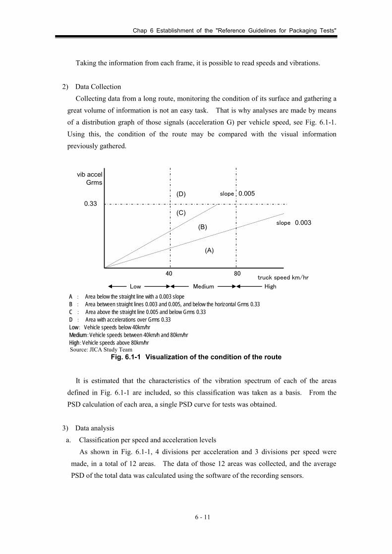
Chap 6 Establishment of the "Reference Guidelines for Packaging Tests"
6 - 11
Taking the information from each frame, it is possible to read speeds and vibrations.
2) Data Collection Collecting data from a long route, monitoring the condition of its surface and gathering a
great volume of information is not an easy task. That is why analyses are made by means of a distribution graph of those signals (acceleration G) per vehicle speed, see Fig. 6.1-1. Using this, the condition of the route may be compared with the visual information previously gathered.
vib accelGrms
0.33(D)
(C)
(B)
(A)
slope 0.005
slope 0.003
truck speed km/hr8040
Low Medium High A : Area below the straight line with a 0.003 slope B : Area between straight lines 0.003 and 0.005, and below the horizontal Grms 0.33 C : Area above the straight line 0.005 and below Grms 0.33 D : Area with accelerations over Grms 0.33 Low: Vehicle speeds below 40km/hr Medium:Vehicle speeds between 40km/h and 80km/hr High:Vehicle speeds above 80km/hr Source: JICA Study Team
Fig. 6.1-1 Visualization of the condition of the route
It is estimated that the characteristics of the vibration spectrum of each of the areas defined in Fig. 6.1-1 are included, so this classification was taken as a basis. From the PSD calculation of each area, a single PSD curve for tests was obtained.
3) Data analysis a. Classification per speed and acceleration levels
As shown in Fig. 6.1-1, 4 divisions per acceleration and 3 divisions per speed were made, in a total of 12 areas. The data of those 12 areas was collected, and the average PSD of the total data was calculated using the software of the recording sensors.
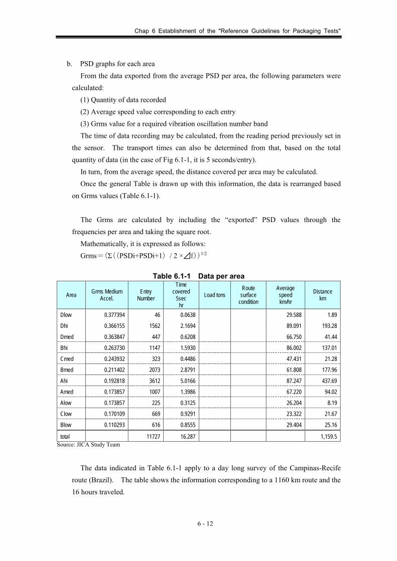
Chap 6 Establishment of the "Reference Guidelines for Packaging Tests"
6 - 12
b. PSD graphs for each area From the data exported from the average PSD per area, the following parameters were
calculated: (1) Quantity of data recorded (2) Average speed value corresponding to each entry (3) Grms value for a required vibration oscillation number band The time of data recording may be calculated, from the reading period previously set in
the sensor. The transport times can also be determined from that, based on the total quantity of data (in the case of Fig 6.1-1, it is 5 seconds/entry).
In turn, from the average speed, the distance covered per area may be calculated. Once the general Table is drawn up with this information, the data is rearranged based
on Grms values (Table 6.1-1). The Grms are calculated by including the “exported” PSD values through the
frequencies per area and taking the square root. Mathematically, it is expressed as follows: Grms=(Σ((PSDi+PSDi+1) / 2 ×⊿f))1/2
Table 6.1-1 Data per area
Area Grms Medium Accel.
Entry Number
Time covered
5sec hr
Load tonsRoute
surface condition
Average speed km/hr
Distance km
Dlow 0.377394 46 0.0638 29.588 1.89
Dhi 0.366155 1562 2.1694 89.091 193.28
Dmed 0.363847 447 0.6208 66.750 41.44
Bhi 0.263730 1147 1.5930 86.002 137.01
Cmed 0.243932 323 0.4486 47.431 21.28
Bmed 0.211402 2073 2.8791 61.808 177.96
Ahi 0.192818 3612 5.0166 87.247 437.69
Amed 0.173857 1007 1.3986 67.220 94.02
Alow 0.173857 225 0.3125 26.204 8.19
Clow 0.170109 669 0.9291 23.322 21.67
Blow 0.110293 616 0.8555 29.404 25.16
total 11727 16.287 1,159.5 Source: JICA Study Team
The data indicated in Table 6.1-1 apply to a day long survey of the Campinas-Recife route (Brazil). The table shows the information corresponding to a 1160 km route and the 16 hours traveled.

Chap 6 Establishment of the "Reference Guidelines for Packaging Tests"
6 - 13
The Grms and distances covered in each of the areas vary. If the vibration levels representing all the stretches could be transformed into hours, the
testing conditions of that stretch could be obtained. As regards criteria, the traditional MIL2 standard was used, the MILSTD-810 was taken
as a reference and data was processed as follows:
c. Calculation method for PSD with compressed time as from the validated average PSD. First, the process will be explained based on the fatigue curve (S-N curve) of materials,
to ease calculation processes. In the fatigue curve, if loads are replaced by “vibration accelerations”, and the number of repetitive oscillations are replaced by the hours covered-testing hours, the relation showed by the curve is maintained, such as it is shown in Fig. 6.1-2. Mathematically, it is expressed as follows:
(W1/W0)M = T0/T1 (1)
W : Level of tests
T : Time elapsed – Testing time
M : Material constant (usually 4)
Here, the following ratio is considered W1/W0=α , amplification factor,
And the ratio T1/T0=λ , is:
αM=1/ λ (1)
Extrapolating to Grms constant.Move the transp.time according to thefatigue characteristics. Calculating
the sum of 4 points
◇
◇
◇◇
× fatigue point
Fatigue characteristic N×σM =constant
(Transp Time per area x Grms)
Factor: Repetitions N-->Transp time
Factor:Stress σ-->Grms
Source: JICA Study Team
Fig. 6.1-2 Validation Criterion
2 Note: Standards of the USA Ministry of Defense usually called MIL Standards. They can also be applied to
civilian uses.
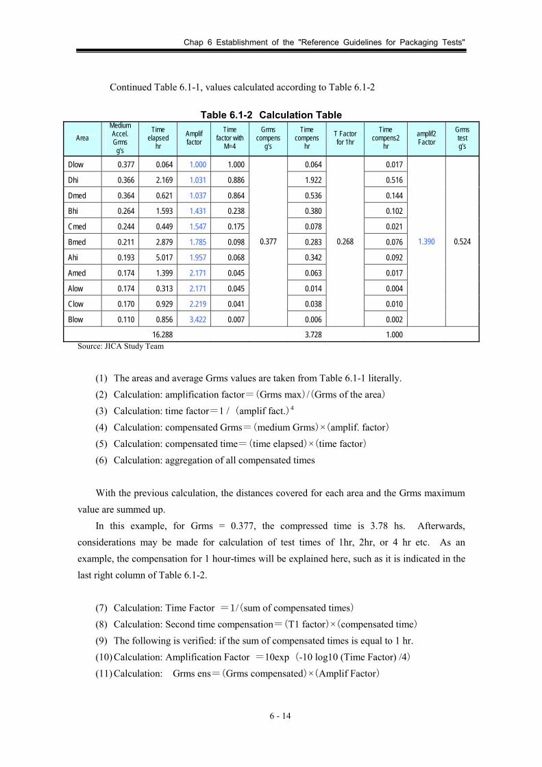
Chap 6 Establishment of the "Reference Guidelines for Packaging Tests"
6 - 14
Continued Table 6.1-1, values calculated according to Table 6.1-2
Table 6.1-2 Calculation Table
Area Medium Accel. Grms
g’s
Time elapsed
hr Amplif factor
Time factor with
M=4
Grms compens
g’s
Time compens
hr T Factor for 1hr
Time compens2
hr amplif2 Factor
Grms test g’s
Dlow 0.377 0.064 1.000 1.000 0.064 0.017
Dhi 0.366 2.169 1.031 0.886 1.922 0.516
Dmed 0.364 0.621 1.037 0.864 0.536 0.144
Bhi 0.264 1.593 1.431 0.238 0.380 0.102
Cmed 0.244 0.449 1.547 0.175 0.078 0.021
Bmed 0.211 2.879 1.785 0.098 0.283 0.076
Ahi 0.193 5.017 1.957 0.068 0.342 0.092
Amed 0.174 1.399 2.171 0.045 0.063 0.017
Alow 0.174 0.313 2.171 0.045 0.014 0.004
Clow 0.170 0.929 2.219 0.041 0.038 0.010
Blow 0.110 0.856 3.422 0.007
0.377
0.006
0.268
0.002
1.390 0.524
16.288 3.728 1.000 Source: JICA Study Team
(1) The areas and average Grms values are taken from Table 6.1-1 literally. (2) Calculation: amplification factor=(Grms max)/(Grms of the area) (3) Calculation: time factor=1 / (amplif fact.)4 (4) Calculation: compensated Grms=(medium Grms)×(amplif. factor) (5) Calculation: compensated time=(time elapsed)×(time factor) (6) Calculation: aggregation of all compensated times
With the previous calculation, the distances covered for each area and the Grms maximum value are summed up.
In this example, for Grms = 0.377, the compressed time is 3.78 hs. Afterwards, considerations may be made for calculation of test times of 1hr, 2hr, or 4 hr etc. As an example, the compensation for 1 hour-times will be explained here, such as it is indicated in the last right column of Table 6.1-2.
(7) Calculation: Time Factor =1/(sum of compensated times) (8) Calculation: Second time compensation=(T1 factor)×(compensated time) (9) The following is verified: if the sum of compensated times is equal to 1 hr. (10) Calculation: Amplification Factor =10exp (-10 log10 (Time Factor) /4) (11) Calculation: Grms ens=(Grms compensated)×(Amplif Factor)
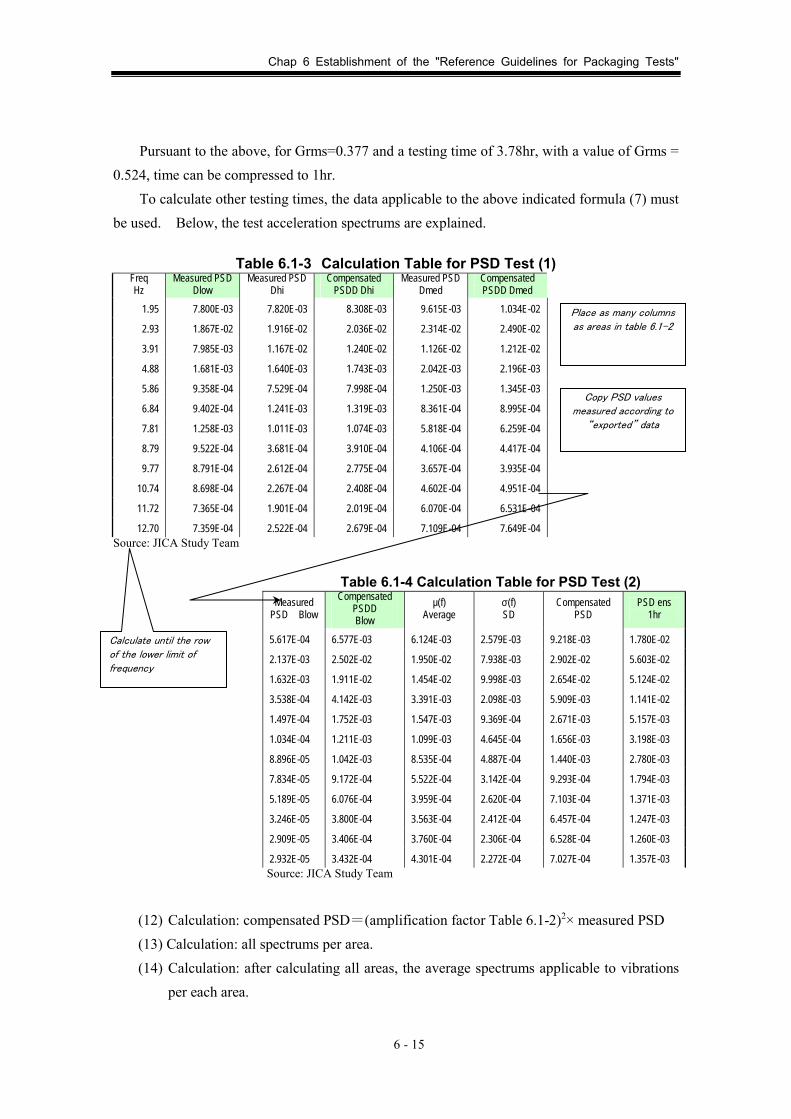
Chap 6 Establishment of the "Reference Guidelines for Packaging Tests"
6 - 15
Pursuant to the above, for Grms=0.377 and a testing time of 3.78hr, with a value of Grms = 0.524, time can be compressed to 1hr.
To calculate other testing times, the data applicable to the above indicated formula (7) must be used. Below, the test acceleration spectrums are explained.
Table 6.1-3 Calculation Table for PSD Test (1)
Freq Hz
Measured PSD Dlow
Measured PSD Dhi
Compensated PSDD Dhi
Measured PSD Dmed
Compensated PSDD Dmed
1.95 7.800E-03 7.820E-03 8.308E-03 9.615E-03 1.034E-02
2.93 1.867E-02 1.916E-02 2.036E-02 2.314E-02 2.490E-02
3.91 7.985E-03 1.167E-02 1.240E-02 1.126E-02 1.212E-02
4.88 1.681E-03 1.640E-03 1.743E-03 2.042E-03 2.196E-03
5.86 9.358E-04 7.529E-04 7.998E-04 1.250E-03 1.345E-03
6.84 9.402E-04 1.241E-03 1.319E-03 8.361E-04 8.995E-04
7.81 1.258E-03 1.011E-03 1.074E-03 5.818E-04 6.259E-04
8.79 9.522E-04 3.681E-04 3.910E-04 4.106E-04 4.417E-04
9.77 8.791E-04 2.612E-04 2.775E-04 3.657E-04 3.935E-04
10.74 8.698E-04 2.267E-04 2.408E-04 4.602E-04 4.951E-04
11.72 7.365E-04 1.901E-04 2.019E-04 6.070E-04 6.531E-04
12.70 7.359E-04 2.522E-04 2.679E-04 7.109E-04 7.649E-04Source: JICA Study Team
Table 6.1-4 Calculation Table for PSD Test (2)
Measured PSD Blow
Compensated PSDD Blow
µ(f) Average
σ(f) SD
Compensated PSD
PSD ens 1hr
5.617E-04 6.577E-03 6.124E-03 2.579E-03 9.218E-03 1.780E-02
2.137E-03 2.502E-02 1.950E-02 7.938E-03 2.902E-02 5.603E-02
1.632E-03 1.911E-02 1.454E-02 9.998E-03 2.654E-02 5.124E-02
3.538E-04 4.142E-03 3.391E-03 2.098E-03 5.909E-03 1.141E-02
1.497E-04 1.752E-03 1.547E-03 9.369E-04 2.671E-03 5.157E-03
1.034E-04 1.211E-03 1.099E-03 4.645E-04 1.656E-03 3.198E-03
8.896E-05 1.042E-03 8.535E-04 4.887E-04 1.440E-03 2.780E-03
7.834E-05 9.172E-04 5.522E-04 3.142E-04 9.293E-04 1.794E-03
5.189E-05 6.076E-04 3.959E-04 2.620E-04 7.103E-04 1.371E-03
3.246E-05 3.800E-04 3.563E-04 2.412E-04 6.457E-04 1.247E-03
2.909E-05 3.406E-04 3.760E-04 2.306E-04 6.528E-04 1.260E-03
2.932E-05 3.432E-04 4.301E-04 2.272E-04 7.027E-04 1.357E-03 Source: JICA Study Team
(12) Calculation: compensated PSD=(amplification factor Table 6.1-2)2× measured PSD (13) Calculation: all spectrums per area. (14) Calculation: after calculating all areas, the average spectrums applicable to vibrations
per each area.
Copy PSD values measured according to
“exported” data
Place as many columns as areas in table 6.1-2
Calculate until the row of the lower limit of frequency

Chap 6 Establishment of the "Reference Guidelines for Packaging Tests"
6 - 16
(15) Calculation: the Standard deviation, such as item (14) above. (16) Calculation: compensated PSD=(Spectrum prom)×1.2 (spectrum standard deviation) This is how the test spectrum is calculated for the whole track. Besides, for the PSD Test
of 1hr we have: (17) Calculation: 1 hr PSD Test =(1hr amplification factor of Table 6.1-2)2×(compensated
PSD item16) (18) Taking the data from the frequency column, the compensated PSD and the 1hr PSD
may be plotted to draw up the spectrum graph.
d. Method to create the PSD Transportation environment surveys in Brazil were carried out in 4 routes using
household appliances supplied by 2 companies. Considering the data collected, the PSD intensities will only be known after comparing the vibration levels, once calculated the testing times and distances. As a first approach, calculations were made by temporarily setting the vibration levels and testing times, as follows:
(1) Define the PSD taking into consideration for 4 days stretch, representing the route. (2) Take 500km-stretches and determine 1hr tests with average vibration values.
e. PSD evolvent curve To show the PSD curve in the vibration test equipment, based on the calculations
showed above, a broken-line graph should be drawn up considering the characteristics of the resulting curve. To this end, the following aspects should be taken into account: (1) The PSD evolvent curve should be drawn up by making the pertinent calculation
verifications, so that the Grms resulting from the calculation based on the PSD evolvent curve would be similar to the original Grms.
(2) At the same time, the displacement and speed levels calculated with the envelope curve should be lower than those admitted by the test devise, based on the usual curves.
(3) Besides, the values cannot exceed the F maximum force of the vibration load of the vibration equipment.
F=1/3(Grms)×(weight of the sample + equipment dynamic load) In case the above mentioned 3 conditions are not fulfilled, the testing time should be
extended and the calculation repeated so that the Grms value would not exceed the indicated value.

Chap 6 Establishment of the "Reference Guidelines for Packaging Tests"
6 - 17
4) Points to be considered in the future Up to now, we have explained one of the ways to create the Reference Guidelines for
Random Vibration Tests of vehicle on the road. Other points should be analyzed, such as treatment of the data collected etc., but the
above is only limited to the reproduction of vibrations in the testing equipment. As regards the administration of the information collected, the procedures for the
planning and verification of tests should be implemented. For example, an effective data control system should be developed, as well as a tool for the determination of effective reference values, based on the size of the different products, the capacities of the testing equipment, the size and type of the vehicles used to transport the goods.
5) Calculation procedures – Examples
The PSD curves calculated based on the data obtained in the 4 Brazilian routes, are the following:
Source: JICA Study Team
Fig. 6.1-3 Case A: Comparison of PSD curves in Brazilian representative 4 routes (reference: 500km distance, testing time 1 hr)
Details of Case-A: (1) The PSD corresponding to a 500km stretch, representative of each of the routes, is
calculated, and in turn, it is converted into the test curve for a 1 hr period. (2) The ASTM curve shows the truck curve, according to the data of the field study.

Chap 6 Establishment of the "Reference Guidelines for Packaging Tests"
6 - 18
In the case of CETEA, this PSD curve is the one frequently used in tests using household fridges, and applied in 6-hour vibration tests.
(3) The red continuous and pointed line is the evolvent line. Both lines show the differences among the 4 routes.
In order to calculate the duration of the test, the 500km may be taken as a reference, and then the proportional value of the route to be analyzed can be calculated.
For example, if for a 3000 km track, the test lasts 6 hours, it can be compared with a 6-hour long ASTM test.
Observations: • The area below 5Hz, if the ASTM curve is considered, does not cover the required level.
In the area between 5 and 20Hz, the situation is reverted.
• In two of the Brazilian routes, high PSD values are observed in the area between 40Hz and higher.
Based on the above description, it may be inferred that with the conventional curve used so far, the test below 5Hz and above 40Hz could not be neither covered not tested.
Source: JICA Study Team
Fig. 6.1-4 Case-B: Comparison of PSD curves in Brazilian representative routes (converted to ref.: distance 500km)
Details of Case -B:

Chap 6 Establishment of the "Reference Guidelines for Packaging Tests"
6 - 19
(1) This is a 2800km route and it was covered in 4 days. The 4 curves corresponded to each day, and they were drawn up by converting the data from an equivalent 500km-route.
(2) The thick black line indicates the total PSD representing the 4 days. (3) In turn, the red line shows the PSD curve for the whole 4 days and converts the 500km
into a 1 hour test.
Distance (km) Time (hr) Day 1 899 13.3 Day 2 863 15.2 Day 3 812 14.0 Day 4 229 5.1
Source: JICA Study Team
Fig. 6.1-5 Case-C: Comparison of PSD curves in Brazilian representative routes (PSD Test Curve)
Details of Case -C: (1) The PSD applicable to the first day is shown. (2) The PSD Test Curves for 1, 2 and 4 hour tests are shown.

Chap 6 Establishment of the "Reference Guidelines for Packaging Tests"
6 - 20
Source: JICA Study Team
Fig. 6.1-6 Case-D: Comparison of PSD curves in Brazilian representative routes (PSD curves pursuant to speed range)
Details of Case-D: (1) As a result of dividing the (Grms) graph in areas, the PSD curves representing each
area are shown here. (2) Each curve of each of the areas is processed for its compensation and the PSD Test
Curve representing all the areas is obtained.
6.1.1 Dropping Tests
Most cargo impact stress during the transport process occur during handling whether by impact o dropping, therefore impacts due to transportation are minimum. That is to say that the human factor is the main cause of impact.
Therefore, load impact ratio will vary to a great extent according to weight, concluding that loads between 5 to 15kgs tend to suffer the hardest impacts.
On the other hand, impacts and droppings may also vary pursuant to other factors, such as the length/width of the cargo, the center of gravity, etc.
If compared to the external weight effort in respect of the product, damages due to impact are considerably higher, and more frequent. This is why drop tests are so important, within the series of tests carried out on packed cargos.
The drop test regulations applied in Japan are two:
• JIS Z0200: General Rules for Evaluation Tests on packed cargo

Chap 6 Establishment of the "Reference Guidelines for Packaging Tests"
6 - 21
• JIS Z0202: Methodology for drop Tests on packed cargos JIS Z0200 standard defines the parameters for tests such as dropping heights, sequences
and number of tests. Standard JIS Z0202 defines the conditions of the equipment to be used in the tests.
For example, in method B of JIS Z0202 standard, in case a packed cargo is subject to impact tests, the equipment required as is specified in JIS Z0119 standard “Methodology for Impact Tests, for the design of Packaging”.
To perform the drop tests, there are available 3 methods:
• Free fall: Products are dropped in the air.
• Fall on corners: The cargo is placed on a platform leaned on one of the corners and dropped to fall on the other corners.
• Impact Method: Using the impact test equipment. (In this Study, the tests are carried out based on the conditions described in Chapter 7 of
this report, using the equipment from the labs of the counterpart institutions and taking samples of the 2 types of “target” products previously selected. )
Regarding to the determination of the Reference Values, they are described in the Chapter 3, clause 3.2.6.5, so that it can be used as reference. However, regarding to the actual data gathering, is necessary a well coordination between all the participants and specially the criteria and the thinking of the managing personnel of the group working for the survey, about how to use the data.
Regarding to the survey of cargo handling, the following aspects must be considered: if the survey will be done openly or confidentially, if both, how to solve the differences aroused in gathered data between one or other method, if data can be used for the determination of the reference value, can the data be useful for the development of the operation environment, the selection of mechanical devices of the works and their maintenance, etc. Depending on the deep comprehension of all these factors, the information emerging from surveyed data could change drastically.
6.1.2 Vibration Tests
Vibration tests are used to assess if the packaging or product is duly protected against damages that may be suffered by oscillations during transport, that may be caused by the means of transport itself (truck, van, vessels, aircrafts, etc.). To that end, vibrations are applied to the cargo under certain conditions and the behavior of such cargo (or product) is then analyzed. As regards the damages due to vibration, they may vary due to the following: the fatigue of materials due to component resonance phenomena, damages due to internal impact between components, lack of adjustment of linking elements such as screws, damages or scratches due to

Chap 6 Establishment of the "Reference Guidelines for Packaging Tests"
6 - 22
friction with the packaging or the product, flattening of the boxes due to the effort made by dynamic phenomena due to vibration. These are the reasons why the damages and the causes of such damages do not always coincide if compared to those observed in the drop tests.
The aim of vibration tests is to basically reproduce the real transportation environment, with the purpose of establishing testing conditions equal the real ones.
New trends in packaging design help to adjust the packaging to protect the cargo against impacts at the minimum required limit, reducing the margin of protection of the cargo against vibration. For this reason, it’s becoming more necessary to further study the levels of protection against vibration, based on the applicable tests to verify packaging under these conditions.
Within the dynamic efforts the cargos are subject to during transportation, handling impacts are low, in the order of 1 digit percentage on the total cargo. This is why, in case the load is barely protected against vibration, the possibility of damage during transportation is high, being necessary to perform thorough vibration tests.
Standards for vibration tests in Japan are 2:
• JIS Z0200: General Rules for Evaluation Tests on packed cargos.
• JIS Z0232: Methodology for vibration tests on packed cargos. The first standard specifies the vibration levels the cargo is subject to, and the duration of
the test. The second standard sets forth the specifications of the equipment used in the test. (In this Study, the testing conditions were set based on the results of the analysis of data
collected in the transportation environment surveys, using the previously selected “target” products, performed in the labs of the counterpart institutions)
Until now, the reference values for transportation vibration tests were normally determined following this procedure: 1) Routes were classified in several categories. 2) Some route stretches of each category were selected. The surveys of these stretches were
prepared. 4) The typical PSD for each type of route was defined. 5) As regards a new route to be studied, a weighted average calculation of each type of route
was made to evaluate the whole route (% for each type). 6) Taking into account these percentages and the level of possible damages due to accumulated
fatigue in materials during transport, the PSD per type of route were combined and the standard curve was determined (But, the PSD curve patterns should be similar. If there are significant differences, new testing conditions should be defined, as many as different patterns).

Chap 6 Establishment of the "Reference Guidelines for Packaging Tests"
6 - 23
In the past, the procedure applied to define the standard PSD consisted in discussing the criteria on how the routes would be divided, classifying them by photographs and exchanging information among the study teams and counterpart institutions.
However, the transportation conditions in each country are different, and it has been difficult to establish a basic common criterion for the classification of routes.
On the other hand, memories have more capacity so data can be collected over a uniform percentage (20%) of the total.
I.e., the information on type of route, structure, etc, that until now was only hypothetical, can now – thanks to all the information collected – be directly evaluated, being highly reliable.
Besides, for the reference PSD per type of route all the information gathered from similar stretches classified into the same category can be used not considering the first one as a “model”. Therefore, the data is now more accurate.
The application of GPS data has permitted the monitoring of routes and the analysis of data with an unprecedented accuracy. Nevertheless, new procedures had to be designed to process all this data. One of these procedures is the one used to classify the data collected according to the type of route. Another important aspect is the availability of the data analysis function within the programs provided by sensor manufacturers.

Chap 6 Establishment of the "Reference Guidelines for Packaging Tests"
6 - 24
6.2 Reference Guideline for Packaging Tests, for Evaluation
6.2.1 Validations up to the date of the Interim Report
Based on the mutual agreement about the methodology for the determination of the "Reference Guideline for Packaging Tests, for Evaluation", reached during the Joint Meeting of 4 member countries, in the occasion of issuing the Progress Report of this Study, (as stated in the Work Plan for the 3rd year of the Study), a series of discussion meetings have been developed. As result of the activities of the Study, through Work Shops, they were obtained energy scatter diagrams i.e. “Grms vs Speed” and “PSD” diagrams for each transportation survey made on routes of each country. The information are ordered sequentially as: Argentina, Brazil, Paraguay and Uruguay.
(1) Diagram of Grms vs truck speed – Argentina
Buenos Aires-Mendoza-1000km
0
0.2
0.4
0.6
0.8
1
1.2
0 20 40 60 80 100
C C-low C-med B-low B-med B-high A-med A-high A-low C-med
Source: JICA Study Team

Chap 6 Establishment of the "Reference Guidelines for Packaging Tests"
6 - 25
(2) Diagram of Grms vs truck speed – Brazil (Campinas-Recife)
Campinas - Recife 24/10/2005
0.00
0.20
0.40
0.60
0.80
1.00
1.20
0 20 40 60 80 100 120
Speed (km/h)
Grm
s
Area 1 Area 2 Area 4 Area 5 Area 6 Area 7 Area 8 Area 9 Area 10 Area 11 Area 12
Source: JICA Study Team
(3) Diagram of Grms vs truck speed – Paraguay
0
0.1
0.2
0.3
0.4
0.5
0.6
0 20 40 60 80 100 120 140
KM/H
GR
MS
AREA1 AREA2 AREA3 AREA4AREA5 AREA6 AREA7 AREA8AREA9 AREA10 AREA12 LIMITE A-BLIMITE B-C
Source: JICA Study Team

Chap 6 Establishment of the "Reference Guidelines for Packaging Tests"
6 - 26
(4) Diagram of Grms vs truck speed – Uruguay (Montevideo Rocha)
Source: JICA Study Team
Based on the above Grms distribution diagrams, the associated PSD diagrams have been
prepared, for each country.
(1) Argentina: Buenos Aires – Mendoza
1.00000E-08
1.00000E-07
1.00000E-06
1.00000E-05
1.00000E-04
1.00000E-03
1.00000E-02
1.00000E-01
1.00000E+00
1 10 100 1000
Psd_A-med Psd_A-high
Source: JICA Study Team

Cha
p 6
Esta
blis
hmen
t of
the
"R
efer
ence
Gui
delin
es f
or P
acka
ging
Tes
ts"
6 - 27
(2)
Bra
zil :
Cam
pina
s – R
ecife
Sour
ce: J
ICA
Stu
dy T
eam
0-0
,11g
's a
nd
0-4
0km
/h
1.0
0E
-07
1.0
0E
-06
1.0
0E
-05
1.0
0E
-04
1.0
0E
-03
1.0
0E
-02
1.0
0E
-01
1.0
0E
-01
1.0
0E
+0
01
.00
E+
01
1.0
0E
+0
21
.00
E+
03
Fre
qu
en
cy
(Hz)
PSD
Grm
s =
0,0
78
g's
0-0
,11g
's a
nd
40-
80k
m/h
1.0
0E
-07
1.0
0E
-06
1.0
0E
-05
1.0
0E
-04
1.0
0E
-03
1.0
0E
-02
1.0
0E
-01
1.0
0E
-01
1.0
0E
+0
01
.00
E+
01
1.0
0E
+0
21
.00
E+
03
Fre
qu
en
cy
(Hz)
PSD
Grm
s =
0,2
62
g's
0,11
-0,2
2g
's a
nd
0-4
0km
/h
1.0
0E
-07
1.0
0E
-06
1.0
0E
-05
1.0
0E
-04
1.0
0E
-03
1.0
0E
-02
1.0
0E
-01
1.0
0E
-01
1.0
0E
+0
01
.00
E+
01
1.0
0E
+0
21
.00
E+
03
Fre
qu
en
cy
(Hz)
PSD
Grm
s =
0,1
56
g's
0,11
-0,2
2g
's a
nd
40
-80k
m/h
1.0
0E
-07
1.0
0E
-06
1.0
0E
-05
1.0
0E
-04
1.0
0E
-03
1.0
0E
-02
1.0
0E
-01
1.0
0E
-01
1.0
0E
+0
01
.00
E+
01
1.0
0E
+0
21
.00
E+
03
Fre
qu
en
cy
(Hz)
PSD
Grm
s =
0,1
79
g's
0,11
-0,2
2g
's a
nd
40
-80k
m/h
1.0
0E
-07
1.0
0E
-06
1.0
0E
-05
1.0
0E
-04
1.0
0E
-03
1.0
0E
-02
1.0
0E
-01
1.0
0E
-01
1.0
0E
+0
01
.00
E+
01
1.0
0E
+0
21
.00
E+
03
Fre
qu
en
cy
(Hz)
PSD
Grm
s =
0,2
15
g's
0,22
-0,3
3g
's a
nd
0-4
0km
/h
1.0
0E
-07
1.0
0E
-06
1.0
0E
-05
1.0
0E
-04
1.0
0E
-03
1.0
0E
-02
1.0
0E
-01
1.0
0E
-01
1.0
0E
+0
01
.00
E+
01
1.0
0E
+0
21
.00
E+
03
Fre
qu
en
cy
(Hz)
PSD
Grm
s =
0,2
44
g's
0,22
-0,3
3g
's a
nd
40
-80k
m/h
1.0
0E
-07
1.0
0E
-06
1.0
0E
-05
1.0
0E
-04
1.0
0E
-03
1.0
0E
-02
1.0
0E
-01
1.0
0E
-01
1.0
0E
+0
01
.00
E+
01
1.0
0E
+0
21
.00
E+
03
Fre
qu
en
cy
(Hz)
PSD
Grm
s =
0,2
39
g's
0,2
2-0
,33g
's a
nd
80-
120
km
/h
1.0
0E
-07
1.0
0E
-06
1.0
0E
-05
1.0
0E
-04
1.0
0E
-03
1.0
0E
-02
1.0
0E
-01
1.0
0E
-01
1.0
0E
+0
01
.00
E+
01
1.0
0E
+0
21
.00
E+
03
Fre
qu
en
cy
(Hz)
PSD
Grm
s =
0,2
56
g's
Ov
er 0
,33
g's
an
d 0
-40k
m/h
1.0
0E
-07
1.0
0E
-06
1.0
0E
-05
1.0
0E
-04
1.0
0E
-03
1.0
0E
-02
1.0
0E
-01
1.0
0E
-01
1.0
0E
+0
01
.00
E+
01
1.0
0E
+0
21
.00
E+
03
Fre
qu
en
cy
(Hz)
PSD
Grm
s =
0,3
52
g's
Ov
er
0,33
g's
an
d 4
0-8
0km
/h
1.00
E-0
7
1.00
E-0
6
1.00
E-0
5
1.00
E-0
4
1.00
E-0
3
1.00
E-0
2
1.00
E-0
1
1.00
E-0
11.
00E
+00
1.00
E+
011.
00E
+02
1.00
E+
03
Fre
qu
en
cy (
Hz)
PSD
Grm
s =
0,3
77g
's
Ove
r 0,
33g
's a
nd
80-
120
km/h
1.0
0E
-07
1.0
0E
-06
1.0
0E
-05
1.0
0E
-04
1.0
0E
-03
1.0
0E
-02
1.0
0E
-01
1.0
0E
-01
1.0
0E
+0
01
.00
E+
01
1.0
0E
+0
21
.00
E+
03
Fre
qu
en
cy
(Hz)
PSD
Grm
s =
0,3
67
g's
40k
80k
120k
0.11
0.22
0.33
Grm
s
S pee
d

Chap 6 Establishment of the "Reference Guidelines for Packaging Tests"
6 - 28
(3) Paraguay: Diagram of PSD for the twelve areas
1,00E-07
1,00E-06
1,00E-05
1,00E-04
1,00E-03
1,00E-02
1,00E-01
1 10 100 1000
FRECUENCIA HZ
PSD1 PSD2 PSD3 PSD4
PSD5 PSD6 PSD7 PSD8
PSD9 PSD10 PSD12
Source: JICA Study Team
(4) Uruguay: PSD Diagram route: Rocha C – Area 1
Source: JICA Study Team
Also, others studies have been developed for the preparation of the "Reference Guideline
for Packaging Tests, for Evaluation" at MERCOSUR level, by using the route classification by Grades, according to route status.
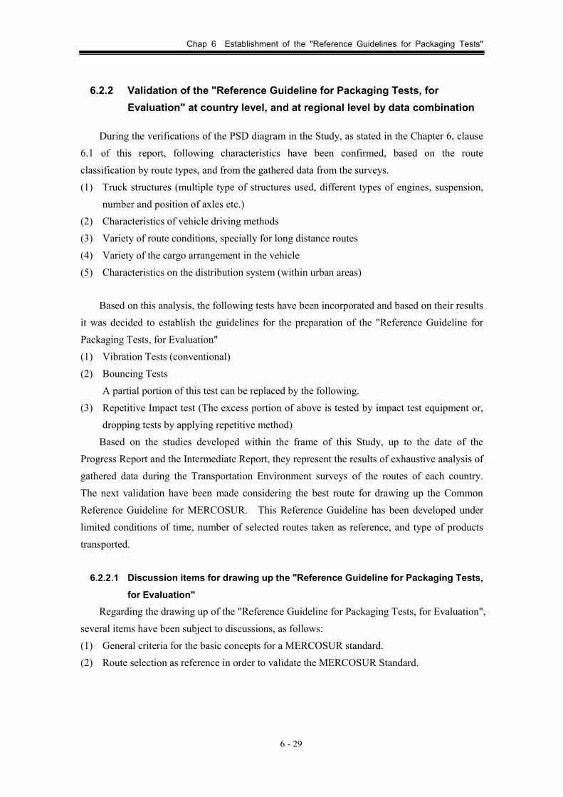
Chap 6 Establishment of the "Reference Guidelines for Packaging Tests"
6 - 29
6.2.2 Validation of the "Reference Guideline for Packaging Tests, for Evaluation" at country level, and at regional level by data combination
During the verifications of the PSD diagram in the Study, as stated in the Chapter 6, clause 6.1 of this report, following characteristics have been confirmed, based on the route classification by route types, and from the gathered data from the surveys. (1) Truck structures (multiple type of structures used, different types of engines, suspension,
number and position of axles etc.) (2) Characteristics of vehicle driving methods (3) Variety of route conditions, specially for long distance routes (4) Variety of the cargo arrangement in the vehicle (5) Characteristics on the distribution system (within urban areas)
Based on this analysis, the following tests have been incorporated and based on their results it was decided to establish the guidelines for the preparation of the "Reference Guideline for Packaging Tests, for Evaluation" (1) Vibration Tests (conventional) (2) Bouncing Tests A partial portion of this test can be replaced by the following. (3) Repetitive Impact test (The excess portion of above is tested by impact test equipment or,
dropping tests by applying repetitive method) Based on the studies developed within the frame of this Study, up to the date of the
Progress Report and the Intermediate Report, they represent the results of exhaustive analysis of gathered data during the Transportation Environment surveys of the routes of each country. The next validation have been made considering the best route for drawing up the Common Reference Guideline for MERCOSUR. This Reference Guideline has been developed under limited conditions of time, number of selected routes taken as reference, and type of products transported.
6.2.2.1 Discussion items for drawing up the "Reference Guideline for Packaging Tests,
for Evaluation"
Regarding the drawing up of the "Reference Guideline for Packaging Tests, for Evaluation", several items have been subject to discussions, as follows: (1) General criteria for the basic concepts for a MERCOSUR standard. (2) Route selection as reference in order to validate the MERCOSUR Standard.

Chap 6 Establishment of the "Reference Guidelines for Packaging Tests"
6 - 30
(3) The combination of data gathered in the 4 member countries, and their analysis.1 Their advantages and calculations development.
(4) Definition of PSD curves for packaging tests, and the conditions for the tests according to the selected cases.
6.2.2.2 Detail discussions and conclusions
(1) General criteria and basic concepts for a MERCOSUR standard 1) The MERCOSUR standard will consider as reference the most recent data gathered from
the developed Transportation Environment Surveys. However, each MERCOSUR standard can be continued in their own development through future revisions of the document, based on new route surveys in each country.
2) This MERCOSUR standard will have as area of application, the member countries of the MERCOSUR. The data to be taken as reference have been divided into two groups – above and below 0.33 Grms- taking into account the results of data analysis of data having very high acceleration values, such as the case of some data gathered in Brazil.
a. The data equal or below 0.33 Grms are evaluated by Vibration Tests. b. The data above 0.33 Grms are evaluated by the Bouncing Tests. (A portion of this test can be replaced by repetitive impact tests)
3) For vibration tests, this standard will consider two types of products for the tests, depending on the characteristics of the product.
Pattern-A: Products subject to damages due to fatigue of the materials (mainly industrial products).
Pattern-B: Products subject to damages due to friction (mainly food products) 4) The frequency ranges for each pattern are defined as follows: Pattern-A: 5 to 100Hz Pattern-B: 3 to 50Hz 5) The overall “PSD Curve for Tests” 2 of packaging is defined as the resultant of
applying all the “PSD Summary curves” 3 of all the 4 member countries. 6) The PSD Curve for Tests for Pattern-A must be drawn so that the lines are closer as
possible to the peaks of PSD Summary curve. The reason of this is because, the products subject to damages due to fatigue are under tests, they can be subject to vibrational stress larger than the actual transportation conditions, due to the application of that simplified PSD curve. Consequently, if the test conditions are different from the physical
1 NdT: From data combination, it is obtained the so called “PSD Summary” curves.
2 NT: PSD Curve for Tests: A broken line in PSD diagram, applicable for laboratory test.
3 NT: PSD Summary curve: The PSD Curve resulting from combining a group of PSD curves.

Chap 6 Establishment of the "Reference Guidelines for Packaging Tests"
6 - 31
requirements of the actual transportation, the results to be obtained in the test also would be very different from those under actual transportation.
On the contrary, the tests for Pattern-B are centered in reproducing the abnormal conditions. Since the friction is associated to vibrations, the important point is that the Curve for Tests must be drawn close to the Summary Curve in the zone of low frequencies. But for the high frequencies, there are no major difficulties to apply a simplied curve, instead.
7) The final PSD Curve for Test will have a margin of ±3dB, so that the expected PSD Curve of actual test must be plotted within this band. It is planned to carry out the verification if the lab test equipment (vibration Test machine) can generate the test conditions according to this PSD curve for Test, by INTI (Argentina).
(2) Reference route selection from surveys, for MERCOSUR common standard The selection of the reference route for MERCOSUR standard is based on the following
criteria. 1) All the surveyed routes up today have been verified (Transportation Environment Surveys)
and a combination of pair of routes from different countries have been set. The verifications have been done for a total of 52 combinations (pairs).
2) Once analyzed the characteristics of all pairs of routes, they were selected the most representative of each category, this means, “good”, “medium”, “bad” routes. The selected pairs of routes are as follows:
Good: BsAs-Rosario(AR)+Montevideo-Rivera(UY) Medium: BsAs-Mendoza(AR)+Loma Plata-Asuncion(PY) Bad: Aimogasta-Iguazu(AR)+Belem-Sao Paulo(BR) Note: The route combinations (pairs) indicated above, does not necessarily represent the actual route for
transportation. These combinations are representative ones for each route category.
(3) Data combination and analysis of gathered data at 4 member countries 1) The data of a pair of route is analyzed. Then, all data above 0.33 Grms are eliminated. 2) The value of Grms is determined and also the test duration based on the data analysis of
remaining data. 3) The Grms values of each route constituent of the pair have a variety. For calculating the
test duration, it is necessary condition that all Grms must be uniform, so that Grms levels of each route must be properly adjusted. That is the reason to make compensation, taking as reference value the Grms maximum.
A Time Factor M is applied, which has defined values depending of type of products: M=4 for industrial products, and M=2 for food products.

Chap 6 Establishment of the "Reference Guidelines for Packaging Tests"
6 - 32
4) Furthermore, the duration related to these data are adjusted by means of another Grms compensation, so that the time of test is compressed. The test duration can be selected from the following values: 1hr, 1.5 hrs, 2 hrs. For this purpose, it was determined that the test must be conditioned so that the accelerations must not be beyond 0.9 G.
5) All the Grms data beyond 0.33 Grms can be analyzed by calculating the number of events for the entire route, based on “time trigger” setting and number of signals gathered. From here, it was determined that precisely this number will be the number of impact to be applied to the sample. This means, the number of jumps on the Bouncing Test. The conditions for the Bouncing Test are 10Hz frequency, 1.1 G acceleration.
6) By calculating the time of test, if this is below 5 minutes, the related time will be a continuous test of 5 minutes.
7) In the case that the test time is above 5 minutes, the excess value can be tested by repetitive shock test by using the impact test apparatus, or the drop test equipment. These repetitive shock tests will be carried out under the following method: in case of applying the impact test apparatus, the speed on the sample is 1.4 m/sec; or in case of free drop test, the drop height will be 10cm. Also, the number of impacts for the repetitive shock test will be 1 impact for each calculated period of 10 minutes.
(4) Definition of PSD Curve for Tests (Standard Curve) 1) Next, it is determined the PSD Curves for Tests. 2) In the case of industrial products, they are suffering the accelerations. In the case of food
products, the containers are subject to the effects depending on the frequency band. Consequently, it is necessary to determine the PSD Curve for Tests, taking into account the type of products to be tested.
3) Therefore, for the PSD curve for tests, the following two curves are defined: Pattern-A: 5 to 100Hz (mainly for industrial products) Pattern-B: 3 to 50Hz (mainly for food products) 4) The Final PSD Curve for Test is determined by compensated Grms curves for the time
compression, considering the container-packaging of each type of product and the frequency ranges.
6.2.3 Results of validation of the Reference Guideline for Packaging Tests, for Evaluation
The general summary of the "Reference Guideline for Packaging Tests, for Evaluation" are described in the Clause 6.3.3 of this report. The guideline and logic process applied in the Clause 6.2.2 are indicated by the following figures. Furthermore, the validation was conducted

Chap 6 Establishment of the "Reference Guidelines for Packaging Tests"
6 - 33
by reanalysis of classified 52 combination data from the Transportation Environment Surveys. The sample calculation and route data figures are shown as follows, and described the leading procedure to the "Reference Guideline for Packaging Tests, for Evaluation" of the MERCOSUR.
Example: Testing Method for a bad conditions route
Source: JICA Study Team
Fig. 6.2.3-1 Grms diagram of a transportation survey, divided into 3 sections

Cha
p 6
Esta
blis
hmen
t of
the
"R
efer
ence
Gui
delin
es f
or P
acka
ging
Tes
ts"
6 - 34
Tabl
e 6.
2.3-
1 R
oute
con
ditio
ns a
nd P
SD C
urve
for T
est
(Exa
mpl
e :
L
oma
Plat
a -A
sunc
ion
rout
e (
PY)
So
urce
: JIC
A S
tudy
Tea
m
Trav
el
Dis
tanc
e Lo
ad
Cap
acity
R
oad
Surf
ace
Con
ditio
n
Mea
n Sp
eed
Trav
elTi
me
Rem
arks
Mea
n ac
cele
ratio
n rms
Trav
el T
ime
Expa
nsio
n C
oeffi
cien
t Ti
me
Coe
ffici
ent
M=4
Col
lect
ion
Valu
e Ti
me
Adju
stm
ent
Tim
eC
oeffi
cien
t Ti
me
Coe
ffici
ent
Tim
eC
oeffi
cien
t R
etim
eAd
just
men
t h
r Ex
pans
ion
Coe
ffici
ent
Ret
ime
Adju
stm
ent
hr
Expa
nsio
n C
oeffi
cien
t Ex
pans
ion
Coe
ffici
ent
Ret
ime
Adju
stm
ent
hr
Test
rms
g's
Test
rms
g's
Test
rms
g's
1-ho
ur a
djus
tmen
t2-
hour
adj
ustm
ent
4-ho
ur a
djus
tmen
t
Actu
al
Mea
sure
men
t PS
D
Actu
al
Mea
sure
men
t PS
DD
Actu
al
Mea
sure
men
t PS
D
Actu
al
Mea
sure
men
t PS
D
Actu
al
Mea
sure
men
t PS
D
Actu
al
Mea
sure
men
t PS
D
Actu
al
Mea
sure
men
t PS
D
Actu
al
Mea
sure
men
t PS
D
Adju
stm
ent
PSD
Ad
just
men
t PS
DD
Ad
just
men
t PS
DD
Ad
just
men
t PS
DD
Ad
just
men
t PS
DD
Ad
just
men
t PS
DD
Ad
just
men
t PS
DD
PS
D
Adju
sted
Va
lue
Test
PS
D4-
hour
Te
st P
SD
2-ho
ur
Test
PS
D1-
hour

Cha
p 6
Esta
blis
hmen
t of
the
"R
efer
ence
Gui
delin
es f
or P
acka
ging
Tes
ts"
6 - 35
Tabl
e 6.
2.3-
2 C
ompa
rison
cal
cula
tion
data
of s
urve
yed
rout
es (e
xam
ple)
So
urce
: JIC
A S
tudy
Tea
m
Com
paris
on o
f Ta
rget
Rou
tes
Rou
tes
Rou
te
Sect
ion
Num
ber
of
Dat
a M
ean
Spee
d km
/hr
Trav
el T
ime
hr
Dat
a Ti
me
hr
Trav
el
Dis
tanc
e
km
Dat
a D
ista
nce
km
Ave.
Grm
s g'
s C
alcu
late
d Ef
fect
ive
Valu
e

Chap 6 Establishment of the "Reference Guidelines for Packaging Tests"
6 - 36
Source: JICA Study Team
Fig. 6.2.3-2 PSD curves for Argentina’s routes
Source: JICA Study Team Fig. 6.2.3-3 PSD curves-comparison of routes : 2 hrs test time

Chap 6 Establishment of the "Reference Guidelines for Packaging Tests"
6 - 37
Source: JICA Study Team
Fig. 6.2.3-4 Measured PSD and Compensated PSD curves (BsAs-Mendoza route, AR)
Test PSD: BsAs - Mendoza
Actual PSD and Normalized: BsAs - Mendoza
Frequency Hz
Frequency Hz
Test PSD 1hr
Test PSD 2hrs
Test PSD 4 hrs
PSD Correction
Normalized

Chap 6 Establishment of the "Reference Guidelines for Packaging Tests"
6 - 38
Source: JICA Study Team Fig. 6.2.3-5 Measured PSD and Compensated PSD curves (PY)
Actual PSD and Normalized PSD: Paraguay
Test PSD: Paraguay
Frequency Hz
Frequency Hz
Test PSD 1hr
Test PSD 2hrs
Test PSD 4 hrs
PSD Correction

Chap 6 Establishment of the "Reference Guidelines for Packaging Tests"
6 - 39
Source: JICA Study Team
Fig. 6.2.3-6 Measured PSD and Compensated PSD curves (Montevideo-Rivera, UY)
Frequency Hz
Frequency Hz
Test PSD: Paraguay: BsAs - Mendoza
Actual PSD and Normalized PSD: BsAs - Mendoza
Test PSD 1hr
Test PSD 2hrs
Test PSD 4 hrs
PSD Correction
Normalized
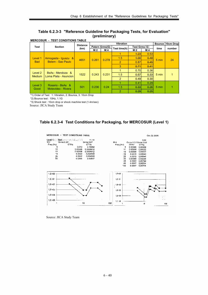
Chap 6 Establishment of the "Reference Guidelines for Packaging Tests"
6 - 40
Table 6.2.3-3 "Reference Guideline for Packaging Tests, for Evaluation" (preliminary)
MERCOSUR - TEST CONDITIONS TABLE Bounce 10cm Drop
M:2 M:4 M:2 M:41 1.23 0.53
1.5 1.00 0.482 0.87 0.453 0.71 0.411 0.70 0.36
1.5 0.57 0.332 0.49 0.301 0.41 0.29
1.5 0.33 0.262 0.29 0.25
*1) Order of Test 1: Vibration, 2: Bounce, 3: 10cm Drop*2) Bounce test : 10Hz, 1.1G*3) Shock test : 10cm drop or shock machine test (1.4m/sec)
Test Section Distance(km) Test time(h)
VibrationTest Grms(G)
BsAs - Mendoza &Loma Plata - Asuncion 1522 5 min
Aimogasta - Iguazu &Belem - Sao Paulo 4651 5 min
0.236 0.24 15 min
1
24
time number
Level 1Bad
Level 2Medium
Level 3Good
Patern Grms(G)
0.261 0.278
0.243 0.231
Rosario - BsAs &Motevideo - Rivera 501
Source: JICA Study Team
Table 6.2.3-4 Test Conditions for Packaging, for MERCOSUR (Level 1)
Source: JICA Study Team
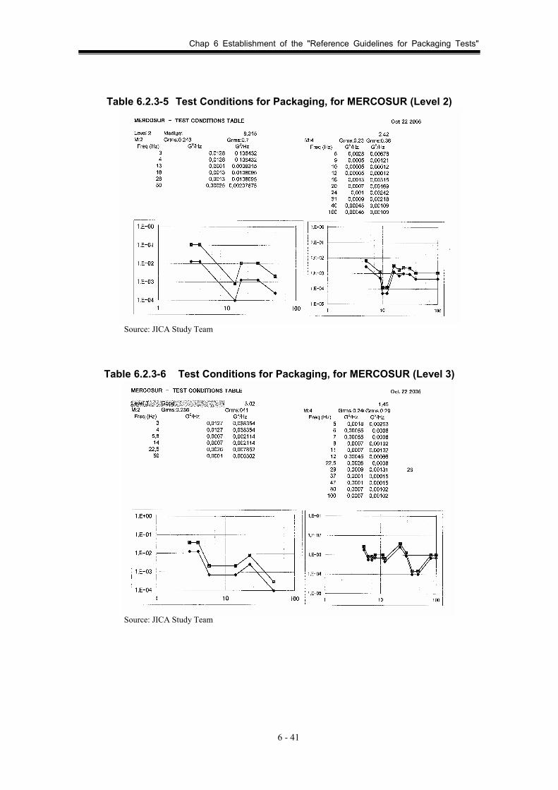
Chap 6 Establishment of the "Reference Guidelines for Packaging Tests"
6 - 41
Table 6.2.3-5 Test Conditions for Packaging, for MERCOSUR (Level 2)
Source: JICA Study Team
Table 6.2.3-6 Test Conditions for Packaging, for MERCOSUR (Level 3)
Source: JICA Study Team