chapter 4.1 - scatter plots and...
TRANSCRIPT

Introduction
Chapter 4.1Scatter plots and correlation
Julian Chan
Department of MathematicsWeber State University
September 15, 2011

Introduction
Intro
1 In statistics we are ultimately interested in collecting data for one of tworeasons:
2 To predict an out come of an event
3 To determine which set of response variables affects to response variable.
Introduction
Intro
1 In statistics we are ultimately interested in collecting data for one of tworeasons:
2 To predict an out come of an event
3 To determine which set of response variables affects to response variable.
Introduction
Intro
1 In statistics we are ultimately interested in collecting data for one of tworeasons:
2 To predict an out come of an event
3 To determine which set of response variables affects to response variable.
Introduction
Intro
1 What is a natural starting point to determine if a relationship existsbetween two variables?
2 Draw a picture!
3 In particular we will draw a scatter diagram. Each individual is representedby a point on the scatter diagram. The explanatory variable is plotted onthe horizontal axis and the response varialbe on the vertical axis.

Introduction
intro
1 A doctor wanted to determine whether a relation exists between a male’sage and his HDL cholesterol. From a simple random sample he obtainedthe following data.

Introduction
Examples
Table: Age and HDL
Age HDL
38 57
42 54
46 34
32 56
55 35
52 40
61 42
61 38
26 47
38 44
66 62
52 48

Introduction
Examples
1 We now provide a scatter plot of the data:

Introduction
Examples
1 We now provide a scatter plot of the data:

Introduction
Example
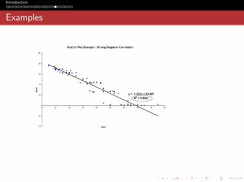
1 The correlation coefficient for the scatter plot above is r = −.2.

Introduction
Example
1 The American black bear is one of eight bear species in the world. It isthe smallest North American bear and the most common bear species. In1969 Dr. Pelton initated a long term study of the population. One aspectof the study was to develop a model that could be used to predict a bearsweight. One variable thought to be related to the bears weight is thelength of the bear.
2 What is the response and explanatory variable?
3 we collect the following data.

Introduction
Examples
Table: Age and HDL
Length(cm) Weigth(Kg)
139 60
138 65
139 68
120.5 50
148 85
141 100
141 90
150 120
166 155
151.5 144
129.5 72
150 148

Introduction
Examples
1 We now provide a scatter plot of the data:

Introduction
Examples
1 We now provide a scatter plot of the data:

Introduction
Example
1 The correlation coefficient for the scatter plot above is r = .85.

Introduction
Examples
1 There are two fundamental differences in the two scatter plots of thedata!
2 One has a slight downward trend and the other has a general upwardtrend!

Introduction
Examples
1 There are two fundamental differences in the two scatter plots of thedata!
2 One has a slight downward trend and the other has a general upwardtrend!

Introduction
Examples
1 A downward trend is what statisticans call a negative association.
2 Two variables that are linearly related are said to be negatively associatedwhen above below average values of one variable are associated to aboveaverage values of the other variable.

Introduction
Examples
1 A downward trend is what statisticans call a negative association.
2 Two variables that are linearly related are said to be negatively associatedwhen above below average values of one variable are associated to aboveaverage values of the other variable.
Introduction
Examples
1 A upward trend is what statisticans call a positive association.
2 Two variables that are linearly related are said to be positively associatedwhen above average values of one variable are associated to aboveaverage values of the other variable.

Introduction
Examples
1 A upward trend is what statisticans call a positive association.
2 Two variables that are linearly related are said to be positively associatedwhen above average values of one variable are associated to aboveaverage values of the other variable.

Introduction
Examples
1 What did you notice about r in the first example?
2 It was negative!
3 What does this reflect?
4 Negative correlation!

Introduction
Examples
1 What did you notice about r in the first example?
2 It was negative!
3 What does this reflect?
4 Negative correlation!

Introduction
Examples
1 What did you notice about r in the first example?
2 It was negative!
3 What does this reflect?
4 Negative correlation!

Introduction
Examples
1 What did you notice about r in the first example?
2 It was negative!
3 What does this reflect?
4 Negative correlation!

Introduction
Examples
1 What did you notice about r in the second example?
2 It was positive!
3 What does this reflect?
4 Positive correlation!

Introduction
Examples
1 What did you notice about r in the second example?
2 It was positive!
3 What does this reflect?
4 Positive correlation!

Introduction
Examples
1 What did you notice about r in the second example?
2 It was positive!
3 What does this reflect?
4 Positive correlation!

Introduction
Examples
1 What did you notice about r in the second example?
2 It was positive!
3 What does this reflect?
4 Positive correlation!

Introduction
Examples
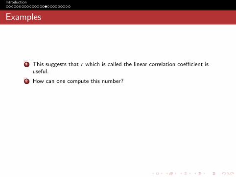
1 This suggests that r which is called the linear correlation coefficient isuseful.
2 How can one compute this number?
r =∑ (xi − x)
Sx
(yi − y)
Sy/(n − 1)
Introduction
Examples
1 This suggests that r which is called the linear correlation coefficient isuseful.
2 How can one compute this number?
r =∑ (xi − x)
Sx
(yi − y)
Sy/(n − 1)

Introduction
Examples
1 This suggests that r which is called the linear correlation coefficient isuseful.
2 How can one compute this number?
r =∑ (xi − x)
Sx
(yi − y)
Sy/(n − 1)

Introduction
Examples
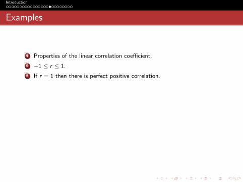
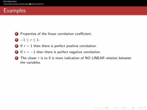
1 Properties of the linear correlation coefficient.
2 −1 ≤ r ≤ 1.
3 If r = 1 then there is perfect positive correlation.
4 If r = −1 then there is perfect negative correlation.
5 The closer r is to 0 is more indication of NO LINEAR relation betweenthe variables.
6 r is not resistant meaning that an observation which does not follow thegeneral pattern of the data can change the value of r !

Introduction
Examples
1 Properties of the linear correlation coefficient.
2 −1 ≤ r ≤ 1.
3 If r = 1 then there is perfect positive correlation.
4 If r = −1 then there is perfect negative correlation.
5 The closer r is to 0 is more indication of NO LINEAR relation betweenthe variables.
6 r is not resistant meaning that an observation which does not follow thegeneral pattern of the data can change the value of r !

Introduction
Examples
1 You tell me. Positive, negative, or no association.
Introduction
Examples

Introduction
Examples

Introduction
examples
1 We practice computing the linear correlation coefficient with the databelow.

Introduction
computation
Table: Age and HDL
Length(cm) Weigth(Kg)
139 60
138 65
139 68
120.5 50
Introduction
example
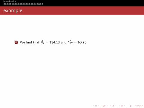
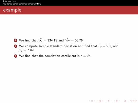
1 We find that XL = 134.13 and YW = 60.75
2 We compute sample standard deviation and find that Sx = 9.1, andSy = 7.89.
3 We find that the correlation coefficient is r = .9.

Introduction
example
1 We find that XL = 134.13 and YW = 60.75
2 We compute sample standard deviation and find that Sx = 9.1, andSy = 7.89.
3 We find that the correlation coefficient is r = .9.
Introduction
example
1 We find that XL = 134.13 and YW = 60.75
2 We compute sample standard deviation and find that Sx = 9.1, andSy = 7.89.
3 We find that the correlation coefficient is r = .9.

Introduction
Example
1 To determine if linear correlation exists between an explanatory variableand a response variable. We compute the abosolute value of r and see ifit is greater than the appropiate value in apendix A table 2.
2 For the length and weight of bears we found above using a smaller dataset that r = .9

Introduction
Example
1 Lurking variables can cause a higher or lower correlation coefficient!
2 A researcher wants to know if drinking cola decreases Bone density inwomen. The data shows that there is negative correlation suggestionevidence for this claim. However, there are a number of lurking variablessuch as other consumption or health factors! This data was also collectedover time therefore it could be the case that naturally these womens donedensity has decreased with age!