chapter 5 high-frequency electromagnetic ﬁ eld coupling to

CHAPTER 5

High-frequency electromagnetic fi eld coupling to long loaded non-uniform lines: an asymptotic approach

S.V. Tkachenko1, F. Rachidi2 & J.B. Nitsch1

1Otto-von-Guericke-University Magdeburg, Magdeburg, Germany.2Ecole Polytechnique Federale de Lausanne, Lausanne, Switzerland.

Abstract

In this chapter, we present and validate an effi cient hybrid method to compute high-frequency electromagnetic fi eld coupling to long loaded lines, when the transmission line approximation is not applicable. The line can contain additional discontinuities (either a lumped impedance or a lumped source) in the central region. In the proposed method, the induced current along the line can be expressed using closed form analytical equations. These expressions involve current waves scattering coeffi cients at the line non-uniformities, which can be determined using either approximate analytical solutions, numerical methods (for the scattering in the line near-end regions), or exact analytical solutions (for the scattering at the lumped impedance in the central region). The proposed approach is compared with numerical simulations and excellent agreement is found.

1 Introduction

The present study considers the important electromagnetic compatibility (EMC) problem of high-frequency electromagnetic fi eld coupling to long transmission lines (TLs). We assume that the frequency spectrum of the exciting fi eld and the transverse dimensions of the line are such that the TL approximation is not applicable. To solve such a problem, one generally resorts to the use of numerical methods (e.g. method of moments) based on the antenna theory. However, a pure numerical method allows to have a general physical picture of the phenomena, only after large series of calcula-tions. Moreover, a systematic use of such methods usually needs prohibitive computer time and storage requirements, especially when analyzing long transmission lines.

www.witpress.com, ISSN 1755-8336 (on-line) WIT Transactions on State of the Art in Science and Engineering, Vol 29, © 2008 WIT Press

doi:10.2495/978-1-84564-063-7/05

160 Electromagnetic Field Interaction with Transmission Lines

Exact analytical expressions of induced current have been developed for the case of infi nite overhead lines [1, 2]. Using those expressions, it has been shown that corrections to TL approximation can be considerable under certain circumstances.

In [3, 4] (see also Chapter 4), a system of equations is derived under the thin-wire approximation describing the electromagnetic fi eld coupling to a horizontal wire of fi nite arbitrary length above the ground plane. The derived equations are in the form of telegrapher’s equations in which the electrodynamics corrections to the TL approximation appear as additional voltage and current source terms. Based on perturbation theory, an effi cient iterative procedure has been proposed to solve the derived coupling equations, where the zeroth iteration term is determined by using the TL approximation (see Chapter 4). However, this method (as formulated in [3, 4]) does not take into account the vertical elements and loads of the wire. Another disadvantage of the method is the divergence of the perturbation series for high-quality-factor systems (e.g. a horizontal open-circuited wire) near the reso-nant frequencies.

In this chapter, we consider the case of a long line, excited by a plane electro-magnetic wave. The line can be terminated at each end by arbitrary impedances (with vertical elements), a confi guration that requires taking into account the inter-actions between wire sections with different directions. The line can contain an additional discontinuity (in the form of a lumped impedance or a lumped source) in the central region.

The proposed hybrid method to compute high-frequency electromagnetic fi eld coupling with a long line will be based on the specifi c features of wave propaga-tion along long wires, as described next. An exciting plane wave generates fast current waves (i.e. with phase velocities larger than the speed of light) along an infi nite straight wire parallel to a perfectly conducting ground. This current wave radiates uniformly along the line [5–10]. When the homogeneity of the line is disturbed by a discontinuity (lumped impedance or lumped source, vertical ele-ments of the line, bend, etc.), the current distribution near the discontinuity becomes more complex, involving different propagation modes, namely trans-verse electromagnetic (TEM) modes, leaky modes (which are attenuated expo-nentially with the distance), and radiation modes (which are attenuated as 1/r n, r being the distance). The exact analytical solution of this problem is known only for the case of a lumped source (lumped impedance) in an infi nite wire (see, e.g. [11–13]), or for the case of a semi-infi nite open-circuited wire [14]. At distances large enough from the discontinuity, in the so-called ‘asymptotic region’, only TEM modes ‘survive’, which propagate along the line without producing any radiation [8, 15, 16]. The amplitude associated with the TEM modes can be expressed in terms of scattering coeffi cients. These TEM modes, in turn, will scatter when reaching line discontinuities, near which, again different type of modes will be present; however, enough distant from the discontinuities in the line asymptotic region, the only ‘surviving’ mode is TEM, and the scattering pro-cess can be described by the refl ection and transmission coeffi cients. To obtain the global solution, we have to consider the scattering associated with each line


High-Frequency Electromagnetic Field Coupling 161

discontinuity and join the solutions in the asymptotic region(s). As a result, we will obtain a closed form analytical expressions for the induced current along the line [5, 6, 17, 18]. These expressions involve scattering coeffi cients for different types of current waves on the line discontinuities, which can be determined using either approximate analytical solutions, numerical methods (for the scattering in the line near–end regions), or exact analytical solutions (for the scattering near a lumped impedance in the central region [18]). The proposed approach will be compared with numerical simulations.

2 High-frequency electromagnetic fi eld coupling to a long loaded line

2.1 Asymptotic approach

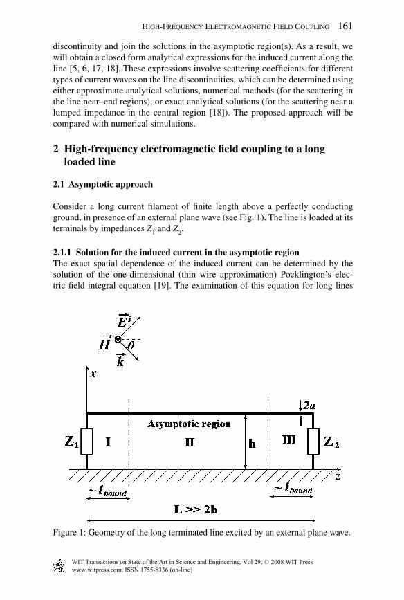
Consider a long current fi lament of fi nite length above a perfectly conducting ground, in presence of an external plane wave (see Fig. 1). The line is loaded at its terminals by impedances Z1 and Z2.

2.1.1 Solution for the induced current in the asymptotic regionThe exact spatial dependence of the induced current can be determined by the solution of the one-dimensional (thin wire approximation) Pocklington’s elec-tric fi eld integral equation [19]. The examination of this equation for long lines

Figure 1: Geometry of the long terminated line excited by an external plane wave.



(L >> 2h) has shown that the current distribution along the line may be divided into three regions as illustrated in Fig. 1 [5]. Regions I and III are located near the terminal loads. The main region II is constituted by portions of the wire suf-fi ciently far from the terminations, i.e. lbound << z << L-lbound. In this central region, called hereafter the asymptotic region, the infl uence of electromagnetic fi elds aris-ing from the load currents may be neglected in comparison with the fi elds gener-ated by the currents along the wire [5]. The value lbound depends rigorously upon the modes generated near the line discontinuities, i.e. lumped loads and vertical elements. However, for most cases of practical interest when kh <≅ 1, a value lbound equal to about 2h can be adopted.

Therefore, we postulate that the general solution for the current along the asymptotic region can expressed as a sum of three distinct terms

0 1 1 2( ) = exp( ) + exp( ) + exp( )I z I jk z I jkz I jkz− − (1)

where k = w/c, and k1 = k cos q, where q is the elevation angle of the incident fi eld (the azimuth angle j = 0).

The fi rst term is a forced response wave, which corresponds to the induced cur-rent on an infi nitely long wire. The second and the third terms are positive and negative travelling waves and the coeffi cients I1 and I2 depend upon the respective geometric wire confi guration and loads at the two line terminals.

The coeffi cient I0 of the forced response wave is determined from the solution of the Pocklilngton’s equation for the case of an infi nitely long wire [19]

2 2 2 e0(d / d + ) ( ) ( )d = 4 ( , ), 1zz k g z z I z z j E h z kae w

∞

−∞

− − π <<′ ′ ′∫

(2)

in which I(z) is the induced current, and g(z) is the scalar Green’s function given by

2 2 2 2+ +4

2 2 2 2

e e( ) =

+ + 4

jk z a jk z h

g zz a z h

− −−

(3)

The term E z e (h,z) is the tangential exciting E-fi eld at the line height, which, for the

case of a vertically polarized plane wave is given by

1 1e 2 sin e( , ) = e (1 e )sin = ( , )ejk z jk zi jkh

z zE h z E E h jq q w− −−−

(4)

The analytical solution for the coeffi cient of the forced wave for the case of a verti-cally polarized exciting fi eld is given by [20] (see also Section 4.2.3)

( )e

0 2 (2)0 0

4 ( , )1= , 1

sin 2 ln sin + 2 sinzcE h j

I kaj ka j j H kh

wwh q g q q

π <<

(2/ ) − π π

(5)

In order to determine the coeffi cients I1 and I2 of the positive and negative travel-ling waves for an arbitrary frequency of the exciting fi eld, it is necessary to know the exact solutions for the induced current in regions I and III, which may be



obtained by solving Pocklington’s equations in these regions using a numerical method (e.g. method of moments). It is worth nothing that Pocklington’s equation uses as source term the tangential component of the exciting electric fi eld along the wire and along the conductors of the load impedances.

To obtain the coeffi cients from the numerical solutions near the line ends, it is necessary to consider an intermediary step, which consists of defi ning two semi-infi nite lines as shown in Fig. 2. (The semi-infi nite line confi gurations will also

Figure 2: Geometry for the original line (a), the right semi-infi nite line (b), and the left semi-infi nite line (c).



allow us to obtain analytical expressions for the induced current near and at the two extremities of the long line, as we shall see in Section 2.1.2.) The right semi-infi nite line extends from the line left-end to +∞ (Fig. 2b), and the left semi-infi nite line extends from −∞ to the line right-end (Fig. 2c). The general solution to this problem can be expressed as a linear combination of the solutions for non-homo-geneous (with external fi eld excitation) and homogeneous (no external excitation) problems.

The non-homogeneous solution for the right semi-infi nite line (0 ≤ z < ∞) and for left semi-infi nite line (–∞ ≤ z ≤ 0) can be expressed respectively as

e e

0( ) = ( )I z I z+ +Ψ (6)

e e

0( ) = ( )I z I z− −Ψ (7)

in which

bounde

1 bound

exact solution in the region, 0( ) =

exp( ) + exp( ),

z lz

jk z C jkz z l++

≤ ≤Ψ − − >>

(8)

and

bounde

1 bound


exp( ) + exp( ),

l zz

jk z C jkz z l−−

− ≤ ≤Ψ − << −

(9)

In eqns (8) and (9), C+ and C– are scattering coeffi cients, which depend on the frequency and the angle of incidence of the exciting electromagnetic fi eld C+ = C+(k,q), C– = C–(k,q).

The homogeneous solution (no external excitation) is given by

0 0( ) = ( )I z z+ +Ψ (10)

0 0( ) = ( )I z z− −Ψ (11)

in which

bound0

bound


exp( ) + exp( ),

z lz

jk z R jkz z l++

≤ ≤Ψ − >>

(12)

and

bound0

bound


exp( ) + exp( ),

l zz

jk z R jkz z l−−

− ≤ ≤Ψ − << −

(13)

In eqns (12) and (13), R+ and R– are the refl ection coeffi cients, which depend on the frequency (R+ = R+(k), R– = R–(k)). It is important to note that both refl ection coeffi cients and scattering coeffi cients are independent of the line length.

Coeffi cients I1 and I2 can be expressed as a function of the coeffi cients C+, C–, R+, and R– by considering that the induced current in the asymptotic region of the



initial line is identical to the current in the asymptotic region for the semi-infi nite lines (see Fig. 2). The general solution for the current in the right semi-infi nite line is given by the sum of homogeneous and non-homogeneous solution

e 0

0 1( ) = ( ) + ( )I z I z I z+ + +Ψ Ψ (14)

in which I0 and I1 are constant coeffi cients.In the asymptotic region of the line, using eqns (8) and (12), the above solution

can be written as

bound 0 1 0 1 1

0 1 1 0 1

( ) = exp( ) + exp( ) + exp( ) + exp( )

= exp( ) + exp( ) +[ + ]exp( )

I z l I jk z I C jkz I jkz I R jkz

I jk z I jkz I C I R jkz

+ + +

+ +

>> − − −

− −

(15)

Similarly, the general solution for the current in the left semi-infi nite line can be written as the sum of non-homogeneous and homogeneous solutions, but consid-ering appropriate argument shifts caused by the new coordinate origin which is shifted by a length L (see Fig. 2c)

e 0

0 1 2( ) = exp( ) ( ) + ( )I z I jk L z L I z L− − −− Ψ − Ψ − (16)

Also in the asymptotic region, we have

bound 0 1 0 1

2 2

0 1 0 1 2

2

( ) = exp( ) + exp( )

+ exp( + ) + exp( )

= exp( )+ exp( ) + exp( )

exp( ) + exp( + )

I z l I jk z I C jkz jkL jk L

I jk z jkL I R jk z jkL

I jk z I C jkL jk L I R jkL

jk z I jk z jkL

− −

−

− −

<< − − − −

− −

− − − − × −

(17)

As it can be seen by eqns (15) and (17), the solution in the asymptotic region is given in the form of the proposed three-term approximation (1). By imposing that the coeffi cients for the terms exp(jkz) and exp(–jkz) are identical in eqns (15) and (17), we obtain a linear system for the unknown coeffi cients I1 and I2, which yields the following solutions:

11 0

exp( ) + exp( 2 )=

1 exp( 2 )

C jkL jk L C R jkLI I

R R jkL− + −

+ −

− − −− −

(18)

12 0

exp( ) + exp( 2 )=

1 exp( 2 )

C jkL C R jkL jk LI I

R R jkL+ − +

+ −

− − −− −

(19)

And, therefore, the coeffi cients I1 and I2 in eqn (1) are given by

11 1 0

exp( ) + exp( 2 )= =

1 exp( 2 )

C jkL jk L C R jkLI I I

R R jkL− + −

+ −

− − −− −

(20)



12 2 0

+ exp( )= exp( ) =

1 exp( 2 )

C C R jkL jk LI I jkL I

R R jkL+ − +

+ −

− −− −

(21)

In this way, the induced current in the asymptotic region II is expressed analytically by eqn (1), in which the coeffi cients, I0, I1, and I2 are given by eqns (5), (20), and (21). The coeffi cients I1 and I2 are expressed in terms of the asymptotic coeffi cients C+, C–, R+, and R–, which are independent of the line length (for a line length larger than a few times its height) and are characterized only by the current scattering near the loads.

For simple line terminal confi gurations such as an open-circuit without vertical elements, these coeffi cients may be obtained analytically using the iteration method presented in Chapter 4. For the general case of arbitrary terminal loads, these coeffi -cients have to be determined numerically (using the method of moments, for instance). Since the asymptotic coeffi cients are independent of the line length, they can be eval-uated using the numerical solutions for signifi cantly shorter lines. In this way, the proposed method makes it possible to compute the response of TL to exciting electro-magnetic fi eld with a reasonable computation time, regardless of the line length.

In order to determine the scattering coeffi cients, it is indispensable to consider two lines because we have to determine four unknowns (C+, C–, R+, and R–), and for each line we have a set of two eqns (20) and (21). Starting from eqns (20) and (21), written for two lines with similar confi gurations (by which we mean the same wire radius, height above ground, terminal impedances, and exciting electromagnetic fi eld), but with signifi cantly shorter lengths L1 and L2, the following expressions for the scattering coeffi cients C+, C–, R+, and R– and can be derived (see Appendix 1)

2 2 2 1

1 2 1 1

( ) ( )=

( ) ( )

I L I LR

I L I L+−−

(22)

2 1 1 2 2 2 1 1

0 1 2 1 1

( ) ( ) ( ) ( )1=

( ) ( )

I L I L I L I LC

I I L I L+−−

(23)

1 2 1 2 1 1 1 1

2 2 1 2 2 1 1 1

( ) exp[ ( ) ] ( ) exp[ ( ) ]=

( )exp[ ( ) ] ( ) exp[ ( ) ]

I L j k k L I L j k k LR

I L j k k L I L j k k L−+ − +− − −

(24)

1 1 2 2 1 1 2 2 1 2

0 2 2 1 1 2 1 1 2

( ) ( ) exp(2 ) ( ) ( ) exp(2 )1=

( )exp[ ( ) ] ( ) exp[ ( ) ]

I L I L jkL I L I L jkLC

I I L j k k L I L j k k L−−

− − −

(25)

2.1.2 Expression for the induced current at the line terminals (regions I and III)

Starting from numerical solutions for the two short line confi gurations I(z,L1) and I(z,L2), it is also possible to derive analytical expressions for the current at the terminals of the original line. The solution in the left-end region (region I in Fig. 1) for the two short lines can be expressed as (from eqn (14))

e 0

1 0 + 1 1( , ) = ( ) ( ) ( )I z L I z I L z+ +Ψ + Ψ (26)



e 0

2 0 1 2( , ) = ( ) + ( ) ( )I z L I z I L z+ + +Ψ Ψ (27)

Note that in the above two equations, the length dependence is contained only in the coeffi cients I1(L1) and I1(L2), which can be calculated by eqn (18). From these two equations, it is possible to infer the functions Ψ + e (z) and Ψ + 0 (z). After some straightforward mathematical manipulations, we get

0 2 1

1 2 1 1

( , ) ( , )( ) =

( ) ( )

I z L I z Lz

I L I L+−

Ψ−

(28)

e 1 1 2 2 1 1

0 1 2 1 1

( , ) ( ) ( , ) ( )1( ) =

( ) ( )

I z L I L I z L I Lz

I I L I L+−

Ψ−

(29)

Inserting the relations (28) and (29) into eqn (14) and considering that I1 = I1, we get the solution for the induced current in the left-end region

1 1 2 2 1 1 2 1left end 1

1 2 1 1 1 2 1 1

( , ) ( ) ( , ) ( ) ( , ) ( , )( , ) | = + ( )

( ) ( ) ( ) ( )

I z L I L I z L I L I z L I z LI z L I L

I L I L I L I L+− −− −

(30)

Similarly, in the right-end region (region III in Fig. 1), the solution for the two short confi gurations can be expressed as (from eqn (16))

e 0

1 0 1 1 1 2 1 1( , ) = exp( ) ( ) + ( ) ( )I z L I jk L z L I L z L− − −− Ψ − Ψ −

(31)

e 0

2 0 1 2 2 2 2 2( , ) = exp( ) ( ) + ( ) ( )I z L I jk L z L I L z L− − −− Ψ − Ψ − (32)

Again in the above two equations, the length-dependence is contained only in coeffi cients I2(L1) and I2(L2), which can be calculated by eqn (19). After some mathematical manipulations, it is possible to inter from these two equations the functions Ψ –

e (z) and Ψ – 0 (z)

0 1 1 1 1 1 2 2 2

1 1 2 1 1 2 2 2

exp( ) ( + , ) exp( ) ( + , )( ) =

exp( ) ( ) exp( ) ( )

jk L I z L L jk L I z L Lz

jk L I L jk L I L−−

Ψ−

(33)

e 1 1 2 2 2 2 2 1

0 1 1 2 2 1 2 2 1

( + , ) ( ) ( + , ) ( )1( ) =

exp( ) ( ) exp( ) ( )

I z L L I L I z L L I Lz

I jk L I L jk L I L−−

Ψ− − −

(34)

Inserting the expressions (33) and (34) into eqn (16) and taking into account that I2 = I2 exp(jkL), we get the solution for the induced current in the right-end region

2 2 2 1 1 1 2 1 2 21

2 2 1 1 2 2 1 1 2 1

1 1 1 1 1 2 2 22

1

|( , ) right end

exp( ) ( ) ( + , ) exp( ) ( ) ( + , )= exp( )

( ) exp( ) ( ) exp( )

exp( ) ( + , ) exp( ) ( + , )+ ( ) exp( )

exp ( )(

I z L

jkL I L I z L L L jkL I L I z L L Ljk L

I L jk L jkL I L jk L jkL

jk L I z L L L jk L I z L L LI L jkL

j k k

−

− − − − −−

− − − − −

− − −−

− 1 2 1 1 2 2 2( ) exp( ( ) ) ( ))L I L j k k L I L− − (35)



2.1.3 Summary of the proposed procedure to determine the induced current along the line and at the line terminals

The procedure for the determination of the coeffi cients of the analytical expres-sions for the induced current along a long line (Fig. 2a) can be summarized as follows:

Apply a numerical method (e.g. method of moments) to compute the response 1. of two equivalent lines having the same confi guration as the initial line, but with shorter lengths L1 << L and L2 << L. Typically, it is enough to consider L1 equal to about 5h and in order to avoid numerical instability, it is desirable to take L2 frequency dependent, for example L2 = L1 + λ/2.

Starting from the numerical solutions for the induced current on the two above-mentioned lines, we determine the coeffi cients I1(L1), I2(L1), I1(L2), I2(L2) using the least-square method.The scattering coeffi cients 2. C+, C–, R+, R– are then computed using eqns (22)–(25).The coeffi cients 3. C+, C–, R+, R–, which are independent of the line length, are used to compute the coeffi cients I1(L), I2(L), for any length L using (20) and (21). The analytical expressions for the induced current along the asymptotic region of the line (1) and at the line ends (30), (35) can be applied for the any line length.

Note that only the fi rst step of the above procedure requires numerical computa-tions, which is to be performed not for the whole line structure but on two signifi -cantly shorter lines. Therefore, the computation time can be drastically reduced for long lines. Additionally, once the numerical solutions for the two short line con-fi gurations are known, it is possible to compute analytically the solution for any similar line confi guration, but with any different line length.

2.2 Accuracy of the proposed three-term expression for the induced current along the asymptotic region of the line

In order to validate our assumption on the analytical form of the induced cur-rent in the asymptotic central region II, we have developed a code for the deter-mination of the coeffi cients I0, I1, I2 in expression (1), starting from numerical solutions obtained using Numerical Electromagnetics Code (NEC) [21]. The real and imaginary parts of coeffi cients I0, I1, I2 were determined separately using the least-square method. It has been shown, considering several load conditions, that the proposed expression (1) approximates very well the spatial dependence of the induced current [6]. An example of comparison between the numerical solutions obtained using NEC with the proposed approximate expression (1) is presented in Fig. 3. The line is characterized by a length L = 16 m, a conductor radius a = 10 mm, and a height above ground h = 0.5 m, and is short-circuited at both ends (Z1 = 0, Z2 = 0). The exciting fi eld is a plane wave with f = 358 MHz (λ = 0.84 m), q = 45°, E0 = 50 kV/m. Note that, the TL approximation is not applicable to this case because the wavelength of the exciting fi eld is practically equal to the height of the conductor above ground. In this fi gure, the abscissa l represents the coordinate



along the whole wire length including the vertical risers, l = 0 corresponding to the point where the vertical conductor touches the ground and l = h to the begin-ning of the horizontal part of the line. The total number of segments along the line considered in the NEC code was Nseg = 245.

It can be seen that an excellent approximation is found in the asymptotic region of the line.

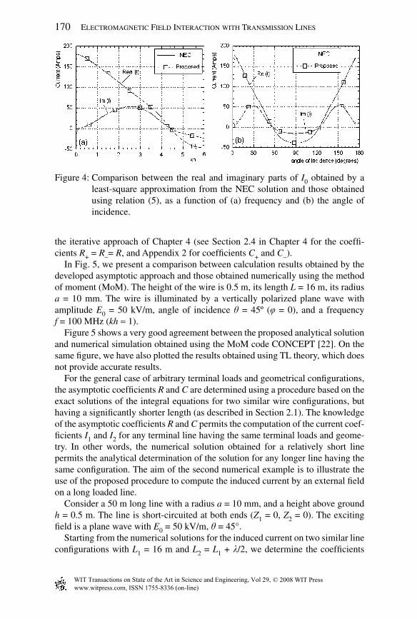
According to our hypothesis, the coeffi cient I0 in the three-term spatial depen-dence (1) should be equal to the expression (5), corresponding to the current induced by an external plane wave for the case of an infi nitely long line. Com-parisons between the real and imaginary parts of I0 obtained from a least-square approximation from the NEC solution and those obtained using relation (5) have also shown an excellent agreement [6]. The results of comparison for the same case of a horizontal wire short-circuited at its both ends are presented in Fig. 4 as a function of the frequency and angle of incidence of the exciting fi eld. Note that the results are practically identical within the resolution accuracy of the drawings.

Other successful tests of the proposed theory were presented in [6] by compar-ing the results to analytical solutions for the case of simple line confi gurations, such as an open-circuit semi-infi nite line.

2.3 Application: response of a long terminated line to an external plane wave

The solution of the coupling equations for long terminated lines using the pro-posed asymptotic theory is illustrated here by two examples.

First, let us consider an open-circuited wire of fi nite length above a perfectly conducting ground (see Fig. 1 in Chapter 4). In this case the exact expressions for the asymptotic coeffi cients can be obtained analytically using the Wiener–Hopf solution [14] (for the coeffi cients R+ = R–= R). They can also be determined using

Figure 3: Comparison of the induced current fl owing along the line using the NEC solution and the proposed approximate formula (1), with coeffi cients determined using the least-square method. Angle of incidence θ = 45°. (a) Real part and (b) imaginary part of the current.



the iterative approach of Chapter 4 (see Section 2.4 in Chapter 4 for the coeffi -cients R+ = R–= R, and Appendix 2 for coeffi cients C+ and C–).

In Fig. 5, we present a comparison between calculation results obtained by the developed asymptotic approach and those obtained numerically using the method of moment (MoM). The height of the wire is 0.5 m, its length L = 16 m, its radius a = 10 mm. The wire is illuminated by a vertically polarized plane wave with amplitude E0 = 50 kV/m, angle of incidence q = 45º (j = 0), and a frequency f = 100 MHz (kh ≈ 1).

Figure 5 shows a very good agreement between the proposed analytical solution and numerical simulation obtained using the MoM code CONCEPT [22]. On the same fi gure, we have also plotted the results obtained using TL theory, which does not provide accurate results.

For the general case of arbitrary terminal loads and geometrical confi gurations, the asymptotic coeffi cients R and C are determined using a procedure based on the exact solutions of the integral equations for two similar wire confi gurations, but having a signifi cantly shorter length (as described in Section 2.1). The knowledge of the asymptotic coeffi cients R and C permits the computation of the current coef-fi cients I1 and I2 for any terminal line having the same terminal loads and geome-try. In other words, the numerical solution obtained for a relatively short line permits the analytical determination of the solution for any longer line having the same confi guration. The aim of the second numerical example is to illustrate the use of the proposed procedure to compute the induced current by an external fi eld on a long loaded line.

Consider a 50 m long line with a radius a = 10 mm, and a height above ground h = 0.5 m. The line is short-circuited at both ends (Z1 = 0, Z2 = 0). The exciting fi eld is a plane wave with E0 = 50 kV/m, q = 45°.

Starting from the numerical solutions for the induced current on two similar line confi gurations with L1 = 16 m and L2 = L1 + l/2, we determine the coeffi cients

Figure 4: Comparison between the real and imaginary parts of I0 obtained by a least-square approximation from the NEC solution and those obtained using relation (5), as a function of (a) frequency and (b) the angle of incidence.



I1(L1), I2(L1), I1(L2), I2(L2) using the least square method. The scattering coeffi -cients C+(jw), C–(jw), R+(jw), R–(jw), are then computed using eqns (22)–(25) as a function frequency. The results are shown in Fig. 6.

It can be seen that for low frequencies (kh << 1), the refl ection coeffi cients R+ and R– tend to 1, which is the TL current refl ection coeffi cient associated with a short-circuit termination. Additionally the scattering coeffi cients C+ and C– tend to zero at low frequencies.

Let us now defi ne the current distribution, for example, for the frequency f ≅ 358 MHz (l = 0.84 m, kh = 3.75). Note that at the considered frequency, the TL approximation is not valid since the wavelength has the same order of magnitude as the line height.

The scattering coeffi cients C+, C–, R+, R– for this frequency are as follows:

= = 0.292 0.327R R j+ − − (36a)

= 1.250 0.291C j+ − (36b)

= 1.004 + 0.402C j− − (36c)

Using eqns (20) and (21) the coeffi cients I1 and I2 for a 50 m long line can be determined as

1( 50m) 65.91 16.1I L j= = − + (37a)

2 ( 50m) 26.25 24.28I L j= = + (37b)

On the other hand, the coeffi cient I0 calculated using eqn (5) is given by

0 = 48.43 4.72I j− − (38)

Figure 5: Current induced along an open-circuited line.



The current along the 50 m long line is simply given by eqn (1) with numeri-cal values for the coeffi cients given by eqns (37) and (38). The results for the induced current in the near end and in the central regions of the line are pre-sented in Fig. 7.

It can be seen that the agreement between the proposed approach and the exact numerical solutions obtained using NEC is very satisfactory. Note that in this fi g-ure, as in Figs 3 and 4, the abscissa l corresponds to the coordinate along the whole wire systems, including the vertical risers.

3 Asymptotic approach for a non-uniform transmission line

The asymptotic approach presented in Section 2.4 can be generalized to calculate the current induced by an incident plane wave along a long line, which has a local discontinuity represented by a series lumped impedance ZL at some intermediate point (see Fig. 8). This problem can describe, for example, a cable with a damaged shield or a shield discontinuity [23].

Figure 6: Variation of the coeffi cients R+, R–, C+, C–, for the horizontal wire short-circuited by vertical risers, as function of frequency.

-1

-0.5

0

0.5

1

1.5

0 0.5 1 1.5 2 2.5 3 3.5 4

Coe

ffic

ient

C-

kh

(d)

(a)

-1

-0.5

0

0.5

1

0 0.5 1 1.5 2 2.5 3 3.5 4

Coe

ffic

ient

R+

kh

Re(R+)Im(R+)

(b)

-1

-0.5

0

0.5

1

1.5

0 0.5 1 1.5 2 2.5 3 3.5 4

Coe

ffic

ient

R-

kh

Re(R-)Im(R-)

(c)

4-1.5

-1

-0.5

0

0.5

1

1.5

0 0.5 1 1.5 2 2.5 3 3.5

Coe

ffic

ient

C+

kh

Re (C+)Im (C+)

Re (C-)Im (C-)



Let us fi rst consider an auxiliary problem represented by Fig. 9, where the line is infi nitely long. The Pocklington’s integral equation, assuming the lumped imped-ance is placed at the coordinate origin z = 0, is given by

22 e

20

1 d+ ( ) ( )d = ( , ) + (0) ( )

4 dz Lk g z z I z z E h z Z I z

j zd

e w

∞

−∞

− −′ ′ ′ π ∫

(39)

Figure 7: Current spatial distribution along a short-circuited horizontal wire (L = 50 m). Comparison between NEC solutions (solid line) and the proposed asymptotic approach (dashed line): (a and b) current in the left-end re-gion; (c and d) current in the central region; (e and f) current in the right-end region. Left columns: real part; right columns: imaginary part.

-200

-100

0

100

200

300

20 22 24 26 28 30

NECProposed

Im(I

) (

Am

ps)

l (m)

-100

-50

0

50

100

150

45 46 47 48 49 50

NECProposed

Re(

I)

(Am

ps)

l (m)

-200

-100

0

100

200

300

45 46 47 48 49 50

NECProposed

Im(I

) (

Am

ps)

l (m)

l (m)

-200

-100

0

100

200

300

0 1 2 3 4 5

Im(I

) (

Am

ps)

NECProposed

-100

-50

0

50

100

0 1 2 3 4 5

NECProposed

Re(

I)

(Am

ps)

l (m)

(a)

(c)

(e)

(b)

(d)

(f)

-100

-50

0

50

100

150

20 22 24 26 28 30

NECProposed

Re(

I)

(Am

ps)

l (m)



where g(z) is the scalar Green’s function given by eqn (3). The lumped impedance, which is usually considered through a boundary condition, is taken into account in eqn (39) as an additional term in the total exiting tangential fi eld E z

t , accounting for the discontinuity at z = 0 [24]

t ez z L= (0) ( )E E Z I zd− (40)

where I(0) is the current in the impedance.Considering that the integration in eqn (39) is carried out over an infi nite inter-

val and that the kernel of the integral-differential equation (39) depends on the difference of arguments z – z', it is possible to fi nd a solution using the spatial Fou-rier transform.

The general solution for an incident plane wave can be written in the form I m e

(z) = I0 y m e (z). The subscript m indicates that the scatterer is placed in the main

Figure 8: Geometry of the long terminated line with an addition lumped impedance.

Figure 9: Infi nitely long line with additional lumped impedance.



central region of the line. y m e (z) is the solution of the non-homogeneous scattering

problem in the main central region of the line. Let us also defi ne:

• y m,+ 0 (z) as the solution in the central region of the homogeneous (no exciting

fi eld) scattering problem for a current (TEM) wave exp(jkz) incident to the load from ∞; and • y m,–

0 (z) as the solution in the central region of the homogeneous scattering prob-

lem for a current (TEM) wave exp(jkz) incident to the load from –∞.

Using the spatial Fourier transform and after mathematical manipulations, it can be shown that

em 1 2( ) = exp( ) + ( )z jk z F zy − (41)

0m, 2( ) = exp( ) + ( )z jkz F zy + (42)

0m, 2( ) = exp( ) + ( )z jkz F zy − −

(43)

in which, the function F2 (z) is

| |L 1

2C L 1

[e + ( /2 ,2 , /2 )]( ) =

2 + [1+ ( /2 ,2 ,0)]

jk zZ F a h kh z hF z

Z Z F a h kh

−−

(44)

and Zc = √_____

m0/e0 (1/2π)ln(2h/a) is the characteristic impedance of the line, and the function F1 is

( )

max20

1 0 2 22 200 0

2 2 ln(1/ ) cos( )( , , ) = 1 d

,

k hy y

F y yj y yG y y

a xa x

a

− π −−

∫

(45)

and

( )( ) ( )

( ) ( )

(2) 2 2 (2) 2 20 0 0 0 0

2 20 0

(2) 2 2 (2) 2 20 0 0 0 0

,

, 2 ln(1/ ),

2 ,

j H y y H y y y y

G y y y y

K y y K y y y y

p a

a a

a

− − − − < − = = − − − >

(46)

It is important to note that the delta-function in eqns (39) and (40) is a mathemati-cal idealization. In reality, the resistive region along the wire has a fi nite length ∆(∆ ≥ a). As far as we are not interested here in the detailed structure of this region, it is possible to limit the integration at the corresponding wave number kmax ≈ π/2∆. In this way, the integration convergence is ensured.



The z-dependence of the second term in eqns (41)–(43) is similar to that of the current induced by a point voltage source in an infi nite wire above a perfectly conducting ground. The corresponding solution can also be easily obtained by the spatial Fourier transform. This problem is a special case of the well-known prob-lem of an infi nite wire above a ground of fi nite conductivity. In [11], a number of papers on this topic were reviewed. Using methods of complex variable functions, it was shown that F2(z) can be represented as the sum of three terms: a main TEM mode, the sum of eigen modes (or leaky modes), and the so-called radiation mode (the anti-symmetrical current modes in the two wire system are presented and investigated in [12, 13]). An investigation of the z-dependence for the function F2(z) shows that for distances from the load larger than about 2h(for kh <~ 1), the transmission line TEM mode exp(–jk|z|) predominates. Other modes decay with the distance from the scattering load as an inverse power of z (radiation mode) or exponentially (eigen modes), i.e. F1(a/2h, 2kh, z/2h)

| |0

z →∞→ .

As a consequence, we can write

em 1 m( ) = exp( ) + exp( | |)z jk z R jk zy − −

(47)

0m, m( ) = exp( ) + exp( | |)z jkz R jk zy + −

(48)

0m, m( ) = exp( ) + exp( | |)z jkz R jk zy − − −

(49)

where Rm is the refl ection coeffi cient given by

Lm

C L 1

=2 + [1+ ( /2 ,2 ,0)]

ZR

Z Z F a h kh−

(50)

In the low-frequency limit, when kh << 1, F1(a/2h, 2kh, 0) Æ 0 (see Fig. 10) and the refl ection coeffi cient reduces to the well-known TL approximation, that is Rm = –ZL/(2ZC + ZL).

Figure 11 shows the variation of the refl ection coeffi cient as a function of kh. It can be seen that at low frequencies (kh << 1), it reduces to the TL value.

Coming back to the fi nite system of Fig. 8, and according to the asymptotic approach, we will search for a solution for the induced current in the following form.

In regions I and II:

e 0

0 1( ) = ( ) + ( )I z I z I zy y+ +

(51)

In regions II–IV:

1 1 e 0 0

0 m 1 2 m, 1 3 m, 1( ) = e ( ) + ( ) + ( )jk LI z I z L I z L I z Ly y y−− +− − −

(52)

where L1 is the distance from the line left-end to the impedance ZL.Also, in regions IV and V:

1 e 0

0 4( ) = e ( ) + ( )jk LI z I z L I z Ly y−− −− −

(53)



Coeffi cients I1, I2, I3, I4 in the above equations can be determined considering an asymptotic view of these solutions in regions II, IV by formulas (8), (9), (12), (13), and (47)–(49) and taking into account that in these regions, the solution can be written using the three-term form (eqn (1)). In this way, approximate analytical solutions for the problem of Fig. 8 can be obtained (see Appendix 3).

Figure 10: Frequency dependence of the function F1 (a/2h, 2kh, 0) for h = 0.5 m, a = 0.01 m, ∆ = 0.04 m.

Figure 11: Frequency dependence of the refl ection coeffi cient Rm (kh), eqn (50), for a/2h = 0.01, ∆ = 4a, ZL = ZC.



To illustrate the proposed asymptotic method, let us consider a simple model of an open-end straight wire above a perfectly conducting ground. The height of the wire is h = 0.5, its length L = 16 m, its radius a = 10 mm. The wire is illuminated by a vertically polarized plane wave with an amplitude E0 = 50 kV/m, angle of incidence q = 45° (j = 0), and a frequency f = 358 MHz. The wire contains an impedance at its centre equal to the characteristic impedance of the line, ZL = ZC. The length of the impedance region is ∆ = 40 mm. In Fig. 12, we show a compari-son between the proposed asymptotic method (eqns (51)–(53) with asymptotic formulas (8), (9), (12), (13), and (47)–(49)) and numerical results obtained using the MoM code CONCEPT [22], for the real and imaginary parts of the induced current.

The refl ection coeffi cients for the current wave at the ends of the line R+ = R– = R, C+, and C_ are obtained using an iterative approach (see Chapter 4 and Appendix 2).

It can be seen that the results obtained using the proposed approach are in excel-lent agreement with ‘exact’ numerical results.

4 Conclusion

We presented in this chapter an effi cient hybrid method to compute electromag-netic fi eld coupling to a long terminated line. The line can also have a discontinuity in the form of a lumped impedance in its central region. The method is applicable for high-frequency excitation for which the TL approximation is not valid.

In the proposed method, the induced current along the line can be expressed using closed form analytical expressions. These expressions involve scattering coeffi cients at the line non-uniformities, which can be determined using either approximate analytical solutions, numerical methods (for the scattering in the line near–end regions), or exact analytical solutions (for the scattering at the lumped

Figure 12: Real and imaginary parts of the induced current along the line. Com-parison between the proposed approach and numerical results obtained using MoM.

160 2 4 6 8 10 12 14-150

-100

-50

0

50

100

150R

e(I(

l)),

A

l, m

CONCEPTAsympt. methodfor line with non-uniformity

CONCEPTAsympt. methodfor line with non-uniformity

-2 0 2 4 6 8 10 12 14 16 18-150

-100

-50

0

50

100

150

Im(I

(l))

, A

l, m



impedance in the central region). The proposed approach has been compared with numerical simulations and excellent agreement is found.

Appendix 1: Determination of coeffi cients R+, R–, C+, C– as a function of coeffi cients I1 and I2

We start from eqns (20) and (21) re-written below

11 0

exp( ) + exp( 2 )( ) =

1 exp( 2 )

C jkL jk L C R jkLI L I

R R jkL− + −

+ −

− − −− −

(A1.1)

12 0

+ exp( )( ) =

1 exp( 2 )

C C R jkL jk LI L I

R R jkL+ − +

+ −

− −− −

(A1.2)

We will fi rst ‘decouple’ the above equations to obtain the separate equations for R+, C+, and for R–, C–. To do that, lets us consider the quantities I2(L)–R+I1(L) and I1(L)–R–I2(L)exp(–2jkL). After straightforward mathematics, it can easily be shown that

2 1 0( ) ( ) =I L R I L I C+ +− (A1.3)

1 2 0 1( ) ( )exp( 2 ) = exp[ ( + ) ]I L R I L jkL I C j k k L− −− − − (A1.4)

Now, let us write eqn (A1.3) for two different line lengths

2 1 1 1 0( ) ( ) =I L R I L I C+ +− (A1.5)

2 2 1 2 0( ) ( ) =I L R I L I C+ +− (A1.6)

It is easy now to express R+ and C+ in terms of I1 and I2

2 2 2 1

1 2 1 1

( ) ( )=

( ) ( )

I L I LR

I L I L+−−

(A1.7)

2 1 1 2 2 2 1 1

0 1 2 1 1

( ) ( ) ( ) ( )1=

( ) ( )

I L I L I L I LC

I I L I L+−−

(A1.8)

Writing eqn (A1.4) for two different line lengths yields

1 1 2 1 1 0 1 1( ) ( )exp( 2 ) = exp[ ( ) ]I L R I L jkL I C j k k L− −− − − + (A1.9)

1 2 2 2 2 0 1 2( ) ( )exp( 2 ) = exp[ ( ) ]I L R I L jkL I C j k k L− −− − − + (A1.10)

And consequently

1 2 1 2 1 1 1 1

2 2 1 2 2 1 1 1

( )exp[ ( ) ] ( )exp[ ( ) ]=

( )exp[ ( ) ] ( )exp[ ( ) ]

I L j k k L I L j k k LR

I L j k k L I L j k k L−+ − +− − −

(A1.11)



1 1 2 2 1 1 2 2 1 2

0 2 2 1 1 2 1 1 2

( ) ( )exp(2 ) ( ) ( )exp(2 )1=

( )exp[ ( ) ] ( )exp[ ( ) ]

I L I L jkL I L I L jkLC

I I L j k k L I L j k k L−−

− − −

(A1.12)

Appendix 2: Derivation of analytical expressions for the coeffi cients C+ and C– for a semi-infi nite open-circuited line, using the iterative method presented in Chapter 4

In this appendix, we use the iterative procedure presented in Chapter 4 to derive an approximate analytical expression of the zeroth and the fi rst iteration terms of the asymptotic coeffi cients C+ and C–, for the case of semi-infi nite open-circuited line (for a right semi-infi nite line (Fig. 2b), the geometry is identical to the one shown in Fig. 1 of Chapter 4, with L Æ ∞). The system is excited by a vertically polarized external electromagnetic wave with an elevation angle q. The azimuth angle of incidence is assumed to be zero, j = 0. For the right semi-infi nite line the solution in the asymptotic region z >> 2h can be expressed as (see Section 2.1.1)

0 1

2( ) (exp( ) exp( ))e

z hI z I jk z C jkz+ +>>

≈ − + −

(A2.1)

where k = w/c, k1 = kcosq and I0 is the current induced on an infi nite line, given by the expression (A2.2), which can easily be derived (see eqn (53) in Chapter 4)

e

0 (2) (2)20 0 0

4 ( )( ) =

sin ( ( sin ) (2 sin ))zcE j

I jH ka H kh

ww

h w q q q−

(A2.2)

where E z e (jw) is the total exciting (incident + ground-refl ected) tangential electric fi eld,

H 0 (2) (x) is the zero order Hankel function of the second kind [25], h0 = √

____ m0e0 .

The zeroth iteration term of the perturbation theory, which is determined by the TL approximation and which satisfi es the open-circuit boundary condition for z = 0, is given by

e

,0 0,0 1( ) = (exp( ) exp( ))I z I jk z jkz+ − − −

(A2.3)

in which I0,0 is the induced current on an infi nite line calculated using TL approxi-mation [20] (eqn (58) in Chapter 4)

e

0,0 20

( , ) 1=

/ 2 ln(2 / ) sinzE h

Ih a j

wm w qπ

(A2.4)

We will derive now an expression for the fi rst iteration term I1(z) using the general equation of the perturbation theory for the nth iteration term (eqn (40) from Chap-ter 4) which reduces, for the right semi-infi nite line (0 ≤ z < ∞, k Æ k – jd, d Æ 0), to the following expression:

e

, 1 1( ) = ( ) (0)exp( )n n nI z F z F jkz+ − −− − (A2.5)



Using the general equation for the function Fn(z) (eqn (41) from Chapter 4) and making use of eqn (A2.3), we can obtain the expression for the function F0(z) for the fi rst iteration

1

2 2 2 2

1

0 0,0

( ) + ( ) +40,0

2 2 2 20

( ) = [e e ]

e ee e d

2 ln(2 / ) ( ) + ( ) + 4

jk z jkz

jk z z a jk z z hjk z jkz

F z I

Iz

h a z z a z z h

− −

∞ − − − −′ ′− ′ − ′

−

− − − ′ − −′ ′

∫

(A2.6)

For small arguments, eqn (A2.6) yields

0 0,0 1(0) =F I D−

(A2.7)

in which

( )1

2 2

1 2 20

exp + 41 exp( )e e d

2 ln(2 / ) + 4

jk jkjk hjk

Dh a h

x xxx

xx x

∞− −

− − ≈ − −

∫

(A2.8)

And, for large arguments z Æ ∞, we get

0 0,0 1 2( ) = exp( )

zF z I jk z D

→∞−

(A2.9)

where

(2)2 0

2= 1 ln( sin ) (2 sin )

2 ln(2 / )

j jD kh H kh

h ag q q

π − − π (A2.10)

To obtain the large argument expressions (A2.9) and (A2.10), we have used the integral (eqn (51)) from Chapter 4 and the well-known formula from the theory of Bessel functions [25]

(2)0

0

2( ) 1 ln( / 2), where = 1.781

z

jH z zg g

→≈ −

π…

(A2.11)

The knowledge of function F0 for z = 0 and z Æ ∞ makes it possible to obtain a closed-form solution in the asymptotic region z >> 2h for the fi rst iteration term of the induced current I1(z). Using eqns (A2.5), (A2.7), and (A2.9), we get

e,1 0,0 2 1 1( ) [ exp( ) + exp( )]

zI z I D jk z D jkz+ →∞

≈ − −

(A2.12)

The total induced current in the asymptotic region is then given by

e e e,0 ,1 0,0 2 1 1

10,0 2 1 1 2

( ) ( ) + ( ) {(1+ )exp( ) + ( 1)exp( )}

= (1+ ){exp( ) + ( 1)(1+ ) exp( )}

zI z I z I z I D jk z D jkz

I D jk z D D jkz

+ + + →∞−

≈ ≈ − − −

− − −

(A2.13)



Now using eqns (A2.2) and (A2.11), and assuming D2 << 1 we can write for the current amplitude

0 0,0 0,0 2

2

1(1+ )

1I I I D

D≈ ≈

− (A2.14)

and eqn (A2.13) becomes

e 1

0 1 1 2( ) {exp( ) + ( 1)(1+ ) exp( )}I z I jk z D D jkz−+ ≅ − − − (A2.15)

Expanding in terms of [2ln(2h/a)]–1 and taking the two fi rst terms, the coeffi cient (D1 – 1)(1 + D2)

–1 in eqn (A2.15) reduces to (D1 + D2 – 1), and eqn (A2.15) becomes

e

0 1 1 2( ) {exp( ) + ( + 1)exp( )}I z I jk z D D jkz+ ≅ − − − (A2.16)

The coeffi cient C+ may be obtained by identifi cation of eqns (A2.1) and (A2.16)

1 21+ +C D D+ ≈ − (A2.17)

The coeffi cient C– can be determined in a similar way considering a semi-infi nite line –∞ < z ≤ 0, for which the current in the asymptotic region z << –2h is given by

e0 1

2( ) (exp( ) + exp( ))

z hI z I jk z C jk z− −<<

≈ −

(A2.18)

It can be easily shown, following similar mathematical development, that the expression for C– is the same as for C+, eqn (A2.17), but replacing k1 by –k1 in eqns (A2.8) and (A2.10).

A comparison of the frequency dependence of the asymptotic current coeffi -cient C(jw) for an open-circuit semi-infi nite line under normal incidence (C+ = C–= C ) obtained by the proposed asymptotic method (Section 2.1.1) and the one derived by iteration method (eqn (A2.17)) is presented in Fig. A2.1, and again, a very good agreement is found.

Appendix 3: Analytical expression for the induced current along the asymptotic region of the line containing a lumped impedance

Let us consider the solution for the current in the asymptotic regions II and IV (see Fig. 7).

In region II, starting from the left end of the line, using the expression (51) and taking into account the asymptotic representation (eqns (8) and (12)), we will get

e 00 1

0 1 12

0 1 1 1

( ) = ( ) + ( )

[exp( ) + exp( )] + [exp( ) + exp( )]

= exp( ) + exp( ) +[ + ]exp( )

z h

I z I z I z

I jk z C jkz I jk z R jkz

I jk z I jkz C I R jkz

y y+ +

+ +>>

+ +

≅ − − −

− −

(A3.1)



Now, starting from the centre of the line, using expression (52), and taking into account the asymptotic representation (eqns (47)–(49)), we will get

1

1 1 1 1 1 1 1

1

1 1

1 1 1 1

e 0 00 m 1 2 m, 1 3 m, 1

( ) ( ) ( ) ( )0 m 2 m

2

( ) ( )3 m

( )0 0 m 2 m 3 m

( ) = e ( ) + ( ) + ( )

e [e + e ]+ [e + e ]

+ [e + e ]

= e +[ e + + (1+ )] e +

jk L

jk L jk z L jk z L jk z L jk z L

L z h

jk z L jk z L

jk z jk L jk z L

I z I z L I z L I z L

I R I R

I R

I I R I R I R

y y y−− +

− − − − − − −

− >>

− −

− − −

− − −

≅

1( )2e jk z LI − −

(A3.2)

As it can be seen from eqns (A3.1) and (A3.2), the solution in the asymptotic region is given in the form of the proposed three-term approximation (1). By imposing that the coeffi cients for the terms exp(jkz) and exp(–jkz) are identical in eqns (A3.1) and (A3.2), we obtain two equations to determine the unknown coef-fi cients I1, I2, and I3

1 1 1 1( )

1 0 m 2 m 3 m= e + e + (1+ )ej k k L jkL jkLI I R I R I R− + − − (A3.3)

1

0 1 2+ = e jkLI C I R I+ +

(A3.4)

Figure A2.1: Comparison of asymptotic coeffi cient for an open-circuit semi-infi nite line obtained by iteration theory (curves 1 and 2) and the one derived by the asymptotic theory (curves 3 and 4). Normal in-cidence.



In a similar way, using the expressions for region IV, we can obtain two other equations for the unknown coeffi cients I1, I2, I3, and I4

1 1( )

3 0 4e = e + ejkL j k k L jkLI I C I R− − + −− −

(A3.5)

1 1 1 1( )

0 m 2 m 3 m 4e + e (1+ ) + e = ej k k L jkL jkL jkLI R I R I R I− (A3.6)

The fi nal solutions for the system of eqns (A3.3)–(A3.6) are given by

2 1 1 1 1

1 1 2 1 1 2

1 2

2 22 0 m m

2 2m m

2 2 2 2 1m m m

= {(1 e )( e + e )

+ (1+ )e ( e + e )}

{(1 e )(1 e ) (1+ ) e }

jkL jkL jk L jkL

jkL jk L jkL jk L jkL

jkL jkL jkL

I I R R C R R

R R C R R

R R R R R R R

− − − −− + +

− − − − −+ − −

− − − −+ − + −

−

× − − −

(A3.7)

1 1 2 1 1 2

2 1 1 1 1

1 2

2 23 0 m m

2 2m m

2 2 2 2 1m m m

= {(1 e )( e + e )

+ (1+ )e ( e + e )}

{(1 e )(1 e ) (1+ ) e }

jkL jk L jkL jk L jkL

jkL jkL jk L jkL

jkL jkL jkL

I I R R C R R

R R C R R

R R R R R R R

− − − − −+ − −

− − − −− + +

− − − −+ − + −

−

× − − −

(A3.8)

1 1

1 2 0= ( e )jkLI I I C A−+ +−

(A3.9)

2 1 1

4 3 0= ( e e )jkL jk LI I I C A− −− +−

(A3.10)

where L2 = L– L1 in eqns (A3.7) and (A3.8).Using the above coeffi cients, the induced current in the asymptotic regions will

be given byIn region II:

1

0 1 2( ) = e + e + ejk z jkz jkzI z I I I− − (A3.11)

In region IV:

1

0 3 4( ) = e + e + ejk z jkz jkzI z I I I− − (A3.12)

where

1 1=I I (A3.13)

2 0 1= +I I C I R+ +

(A3.14)

1( )

3 0 4= e + ejk k k L jkLI I C I R− + −− −

(A3.15)

4 4= e jkLI I (A3.16)



References

Tesche, F.M., Comparison of the transmission line and scattering models [1] for computing the NEMP response of overhead cables. IEEE Trans. on Electromagnetic Compatibility, 34(2), pp. 93–99, 1992.Bridges, G.E.J. & Shafai, L., Plane wave coupling to multiple conductor [2] transmission line above lossy earth. IEEE Trans. on Electromagnetic Com-patibility, 31(1), pp. 21–33, February 1989.Tkatchenko, S., Rachidi, F. & Ianoz, M., A time domain iterative approach [3] to correct the transmission line approximation for lines of fi nite length. Int. Symposium on Electromagnetic Compatibility, EMC ’94 Roma, 13–16 September 1994.Tkatchenko, S., Rachidi, F. & Ianoz, M., Electromagnetic fi eld coupling to [4] a line of fi nite length: theory and fast iterative solutions in frequency and time domains. IEEE Trans. on Electromagnetic Compatibility, 37(4), pp. 509–518, 1995.Tkatchenko, S., Rachidi, F., Ianoz, M. & Martynov, L.M., Exact fi eld-to- [5] transmission line coupling equations for lines of fi nite length. Int. Symposium on Electromagnetic Compatibility, EMC ’96 Roma, 17–20 September 1996.Tkatchenko, S., Rachidi, F., Ianoz, M. & Martynov, L., An asymptotic ap- [6] proach for the calculation of electromagnetic fi eld coupling to long ter-minated lines. Int. Symposium on Electromagnetic Compatibility, EMC’98 ROMA, pp. 605–609, 14–18 September 1998.Agrawal, A.K., Price, H.J. & Gurbaxani, S.H., Transient response of multi- [7] conductor transmission lines excited by a nonuniform electromagnetic fi eld. IEEE Trans. on Electromagnetic Compatibility, EMC-22(2), pp. 119–129, 1980.Markov, G.T. & Chaplin, A.F., [8] The Excitation of Electromagnetic Waves, Radio i Sviaz: Moscow, 1983 (in Russian).Nitsch, J. & Tkachenko, S., Complex-valued transmission-line parameters [9] and their relation to the radiation resistance. IEEE Transaction on Electro-magnetic Compatibility, EMC-47(3), pp. 477–487, 2004.Nitsch, J. & Tkachenko, S., Telegrapher equations for arbitrary frequencies [10] and modes-radiation of an infi nite, lossless transmission line. Radio Sci-ence, 39, RS2026, doi:10.1029/2002RS002817, 2004.Olsen, R.G., Young, G.L. & Chang, D.C., Electromagnetic wave propaga-[11] tion on a thin wire above earth. IEEE Transaction on Antennas and Propa-gation, AP-48(9), pp. 1413–1419, 2000.Marin, L., Transient electromagnetic properties of two parallel wires. [12] Sensor and Simulation Notes, Note 173, March 1973.Leviatan, Y. & Adams, A.T., The response of two-wire transmission line [13] to incident fi eld and voltage excitation including the effects of higher or-der modes. IEEE Transactions on Antennas and Propagation, AP-30(5), pp. 998–1003, September 1982.



Weinstein, L.A., [14] The Theory of Diffraction and the Factorization Method, Chapter VI, Golem, 1969.Collin, R.E., [15] Field Theory of Guided Waves, IEEE Press: New York, 1991.Nitsch, J. & Tkachenko, S., Source dependent transmission line param-[16] eters – plane wave vs TEM excitation. IEEE International Symposium on Electromagnetic Compatibility, Istanbul, Turkey (CD), 11–16 May 2003.Tkachenko, S., Rachidi, F. & Ianoz, M., High-frequency electromagnetic [17] fi eld coupling to long terminated lines. IEEE Transaction on Electromag-netic Compatibility, 43(2), pp. 117–129, 2001.Tkachenko, S., Rachidi, F., Nitsch, J. & Steinmetz, T., Electromagnetic [18] fi eld coupling to non-uniform transmission lines: treatment of discontinui-ties. 15th Int. Zurich Symposium on EMC, Zurich, pp. 603–607, 2003.Tesche, F.M., Ianoz, M. & Karlsson, T., [19] EMC Analysis Methods and Com-putational Models, John Willey and Sons: New York, October 1996.Vance, E.F., [20] Coupling to Shielded Cables, Wiley: New York, 1978.Burke, G.J., Poggio, A.J., Logan, I.C. & Rockway, J.W., Numerical [21] electro-magnetics code – a program for antenna system analysis. Inter-national Symposium on Electromagnetic Compatibility, Rotterdam, May 1979.Singer, H., Brüns, H.-D., Mader, T., Freiberg, A. & Bürger, G.: CONCEPT [22] II User Manual. TUHH, 1997.Rachidi, F., Tesche, F.M. & Ianoz, M., Electromagnetic coupling to cables [23] with shield interruptions. 12th Int. Symp. on EMC, Zurich, February 1997.Leontovich, M. & Levin, K. On the theory of excitation of oscillations in [24] wire antennas. Journal of Technical Physics, XIV(9), pp. 481–506, 1946 (in Russian).Abramowitz, M. & Stegun, I., [25] Handbook of Mathematical Functions, Dower publications: New York, 1970.


chapter 5 high-frequency electromagnetic ﬁ eld coupling to

Documents