chapter 5 landau theory of the fermi liquideduardo.physics.illinois.edu/phys561/fl.pdf · chapter 5...

Chapter 5

Landau Theory of the Fermi

Liquid

5.1 Adiabatic Continuity

The results of the previous lectures, which are based on the physics of non-interacting systems plus lowest orders in perturbation theory, motivates thefollowing description of the behavior of a Fermi liquid at very low tempera-tures. These assumptions (and results) are usually called the Landau Theoryof the Fermi Liquid, or more commonly Fermi Liquid Theory (FLT).1

| ~k |pF

n(~k)

Z

1

Figure 5.1: Discontinuity in the occupation number at the Fermi surface ina a free and in an interacting system.

The physical picture is the following. In the non-interacting system, thespectrum consists of particles and holes with a certain dispersion (the free

1We will follow closely the treatment in Baym and Pethick.

1

2 CHAPTER 5. LANDAU THEORY OF THE FERMI LIQUID

one-particle spectrum) ε0(p). These excitations are infinitely long-lived sincethey cannot decay in the absence of matrix elements (interactions). Theground state is characterized by a distribution function n0(~p) which at T = 0has the form shown in Fig. (5.1).

Landau reasoned that what interactions do is to produce (virtual) particle-hole pairs. Thus, the distribution function must change: n0(~p) → n(~p). Hefurther assumed that this change is a smooth function (i.e. analytic) ofthe interaction. In other words, as the interactions are slowly turned on,the non-interacting states are assumed to smoothly and continuously evolveinto interacting states, and that this evolution takes place without hittingany singular behavior. Such a singularity would signal an instability of theground state and should be viewed as a phase transition. Thus, if thereare no phase transitions, there should be a smooth connection between non-interacting and interacting states. In particular the quantum numbers usedto label the non-interacting states should also be good quantum numbersin the presence of interactions. The one-electron (particle) state becomes aquasiparticle which carries the same charge (−e) and spin (±1/2) of the bareelectron.

Non-interacting Interacting

• electron (particle) |p| > PF →

• hole (|p| < PF )

• charge ±e, spin 12

• always stable

• quasiparticle |~p| > pF

• quasihole |~p| < pF

• charge ±e, spin 12

• stable only at low en-ergies (ω → 0)

The state of the interacting systems can be parameterized by the actual

distribution function n(~p). Let δn(~p) ≡ n(~p) − n0(~p). For the system to bestable δn(p) must be non-zero only for |~p| ≈ pF and the ground state energyis determined by δn(p). If n0(p) → n(p) = n0(p) + δn(p) with δn/n ≪ 1(forall ~p close to the fermi surface), the total energy isE = E0 + δE and we canexpand the excitation energy δE in powers of the change of the distributionfunction δn(~p) as

δE =∑

p

εp δn(p) + · · · (5.1)

The excitation energy δE should also tell us how much energy does itcost to add an excitation of momentum ~p close to the Fermi surface. Thus,

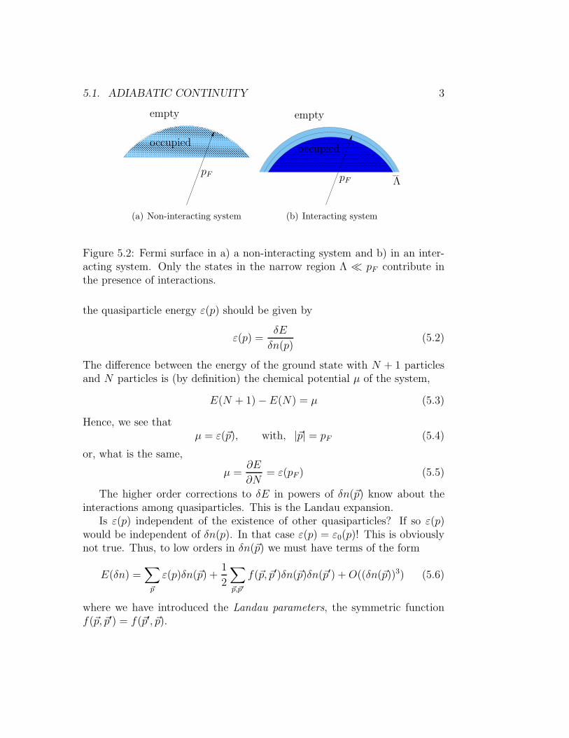
5.1. ADIABATIC CONTINUITY 3

empty

pF

occupied

(a) Non-interacting system

empty

pF

occupied

Λ

(b) Interacting system

Figure 5.2: Fermi surface in a) a non-interacting system and b) in an inter-acting system. Only the states in the narrow region Λ ≪ pF contribute inthe presence of interactions.

the quasiparticle energy ε(p) should be given by

ε(p) =δE

δn(p)(5.2)

The difference between the energy of the ground state with N + 1 particlesand N particles is (by definition) the chemical potential µ of the system,

E(N + 1) − E(N) = µ (5.3)

Hence, we see thatµ = ε(~p), with, |~p| = pF (5.4)

or, what is the same,

µ =∂E

∂N= ε(pF ) (5.5)

The higher order corrections to δE in powers of δn(~p) know about theinteractions among quasiparticles. This is the Landau expansion.

Is ε(p) independent of the existence of other quasiparticles? If so ε(p)would be independent of δn(p). In that case ε(p) = ε0(p)! This is obviouslynot true. Thus, to low orders in δn(~p) we must have terms of the form

E(δn) =∑

~p

ε(p)δn(~p) +1

2

∑

~p,~p′

f(~p, ~p′)δn(~p)δn(~p′) + O((δn(~p))3) (5.6)

where we have introduced the Landau parameters, the symmetric functionf(~p, ~p′) = f(~p′, ~p).


Near |~p| = pF the Fermi velocity is given by ~vF (~~p) = ∂~pε(~p). Hence, wecan define an effective mass

m∗ =pF

|~vF (pF )|(5.7)

which is isotropic only if the Fermi surface is isotropic.

Hence we conclude that ε(p) , which is defined by

ε(p) =δE

δn(p)(5.8)

has the form

ε(p) = ε0(p) +∑

~p′

f(~p, ~p′)δn(~p′) + · · · (5.9)

The correction term gives a measure of the change of the quasiparticle energydue to the presence of other quasiparticles. The function f(~p, ~p′) measuresthe strength of quasiparticle-quasiparticle interactions. Hence f(~p, ~p′) is aneffective interaction for excitations arbitrarily close to the Fermi surface.

What about spin effects? If the system is isotropic and there are nomagnetic fields present, the quasiparticle with up spin (↑) has the sameenergy as the quasiparticle with down spin (↓). Hence ε↑(~p) = ε↓(~p) (Note:This relation is changed in the presence of an external magnetic field by theZeeman effect).

Likewise, the interactions between quasiparticles depends only on therelative orientation of the spins σ and σ′. The Landau interaction term ismodified by spin effects as

∑

~p,~p′

f(~p, ~p′)δn(~p) δn(~p′) →∑

~p,~p′

∑

σ,σ′

fσσ′(~p, ~p′)δnσ(~p)δnσ(~p′) (5.10)

By symmetry considerations we expect that

f↑↑ =f↓↓ ≡ f (S) + f (A)

f↑↓ =f↓↑ ≡ f (S) − f (A)(5.11)

Thus we can also write the quasiparticle interaction term as the sum of a

5.1. ADIABATIC CONTINUITY 5

symmetric and an antisymmetric (or exchange) term∑

~p,~p′

∑

σ,σ′

fσσ′(p, p′)δnσ(p) δnσ′(p′) =

symmetric →∑

~p,~p′

f (S)(p, p′)(δn↑(p) + δn↓(p))(δn↑(p′) + δn↓(p

′)) +

antisymmetric →∑

~p,~p′

f (A)(p, p′)(δn↑(p) − δn↓(p))(δn↑(p′) − δn↓(p

′))

(5.12)

The density of quasiparticle states at Fermi surface, N(0), is

N(0) =1

V

∑

~p,σ

δ(ε0~pσ − µ) = −

1

V

∑

~pσ

∂n0~pσ

∂ε~pσ(5.13)

where we have used the fact that n0~p,σ is the fermi function at T = 0 (a step

function). Hence, we find

N(0) =m∗pF

π2~3(5.14)

where m∗ is the effective mass. To avoid confusion, note that ε0~pσ repre-

sents energy of quasiparticles at the Fermi-surface, while ε0(p) represents theenergy of the non-interacting system, as indicated previously. In a generalscenario, where all of the quasiparticle spins are not quantized along the sameaxis, the spin polarization of the Fermi liquid is (in the following equationsτ represents Pauli matrices, and α, α represents the matrix indices)

σi =∑

p

∑

αα

(τi)αα[n(~p)]αα (5.15)

Equivalently,

n(~p) =1

2

∑

α

(n~p)αα (5.16)

and

~σ(~p) =1

2

∑

αα

(~τ )αα · [n(~p)]αα (5.17)

Consequently

δ2E =1

V 2

∑

pp′

∑

ααα′α′

f~pαα,~p ′α′α′(δn(p))αα(δn(p′))αα (5.18)


wheref~pαα,~p′α′α′ = fS

~p~p′δααδα′α′ + fA~p~p′~ταα~τα′α′ (5.19)

which can also be written more compactly as

f~p~p′ ≡ f(S)pp′ + f

(A)pp′ ~τ · ~τ (no trace) (5.20)

For a rotationally invariant system, the interaction functions fS,A~p,~p ′ must de-

pend only on the angle θ defined by

cos θ(~p, ~p ′) =~p · ~p ′

p2F

(5.21)

Hence we should be able to use an expansion of the form

fS,A~p,~p ′ =

∞∑

ℓ=0

fS,Aℓ Pℓ(cos θ) (5.22)

where

fS,Al =

2ℓ + 1

2

∫ 1

0

dxPℓ(x)1

2(f~p↑,~p ′↑ ± f~p↑,~p ′↓) (5.23)

which leads to the definition of the Landau parameters in terms of angularmomentum channels

F S,Aℓ ≡ N(0)fS,A

ℓ (5.24)

5.2 Equilibrium Properties

5.2.1 Specific Heat:

The low temperature specific heat of a Fermi liquid, just as in the caseof non-interacting fermions, is linear in T with a coefficient determined bythe effective mass m∗ of the quasiparticles at pF . Let’s compute the lowtemperature entropy, or rather the variation of the quasiparticle entropy(per unit volume) as T → T + δT

S = −kB

V

∑

~pσ

[nσ(~p) ln nσ(~p) + (1 − nσ(~p)) ln(1 − nσ(~p))] (5.25)

where nσ(~p) is the Fermi-Dirac distribution

nσ(~p) =1

e(εσ(~p)−µ)/kBT + 1(5.26)

5.2. EQUILIBRIUM PROPERTIES 7

and εσ(~p) is the quasiparticle excitation energy, i.e.,

δF

δnσ(~p)= εσ(~p) (5.27)

where F (δn(~p) is the free energy.Thus, the variation of the entropy is

δS =1

TV

∑

~pσ

(εσ(~p) − µ)δnσ(~p) (5.28)

where

δnσ(~p) =∂nσ(~p)

∂εσ(~p)

[

−(εσ(~p) − µ)

TδT + δεσ(~p) − δµ

︸︷︷︸

]

(5.29)

where the term in braces is due to the quasiparticle interactions. Here,contribution from the first term is

δS1 = −1

V

∑

~pσ

∂nσ(~p)

∂εσ(~p)(εσ(~p) − µ)

δT

T 2(5.30)

Since ∂nσ(~p)∂εσ(~p)

is non-zero only within kBT of the Fermi energy, we find

δS = −∑

σ

∫

p2dp

dε

4π

(2π~)3dε

∂

∂ε

[1

e(ε−µ)/kBT + 1

](ε − µ

T

)2

δT

≡ −k2BN(0)

∫ +∞

−∞

dx∂

∂x

(1

ex + 1

)

x2δT

(5.31)

Hence we find that the low temperature contribution of the quasiparticles is(to leading order) given by

S1 =π2

3N(0)k2

BT (5.32)

and that the specific heat is

Cv = T

(∂S

∂T

)

V

= S1 =π2

3N(0)k2

BT =m∗pF

3~3k2

BT (5.33)


We now introduce the Fermi temperature

TF =p2

F

2m∗kB≡

εF

kB(5.34)

as the Fermi energy in temperature units, in terms of which the specific heatbecomes

CV =π2

2nkB

T

TF=

π2

3

T

TFC0

V (5.35)

where C0V = 3

2nkB is the specific heat of a classical ideal gas, and n is the

particle density.

Using these results we find that the low temperature correction to theFree Energy, F = E − TS, is δF ≈ −SδT (to lowest order), i.e.,

F ≈ E0 −π2

4nkB

T 2

TF

(5.36)

where E0 is the ground state energy. The chemical potential µ is (note thatTF is a function of m∗ and hence a function of n)

µ(n, T ) = −

(∂F

∂n

)

T

= µ(n, 0) −π2

4kB

(1

3+

n

m∗

∂m∗

∂n

)T 2

TF(5.37)

Let us now compute the compressibility:

κ = −1

V

∂V

∂P=

1

n2

∂n

∂µ(5.38)

where P is the pressure. At T = 0,


∂εσ(~p)(δεσ(~p) − δµ) (5.39)

The quasiparticle energy εσ(~p) depends on µ only through its dependence onδnσ′(~p′) (i.e., quasiparticle interactions, see Eq. 5.9). As T → 0 both ∂n

∂εand

δnσ(p) vanish unless all momenta are at the Fermi-surface.

δεσ(p) = fS0

1

V

∑

σ′,~p′

δnσ′(~p′) ≡ fS0 δn (5.40)

5.3. SPIN SUSCEPTIBILITY 9

where fS0 is Landau parameter with with l = 0. Hence, we have


∂εσ(~p)(fS

0 δn − δµ) (5.41)

and

δn =1

V

∑

σ,~p

δnσ(~p) =1

V

∑

σ,~p

∂nσ(~p)

∂εσ(~p)(fS

0 δn − δµ) (5.42)

Similarly,∂nσ(~p)

∂εσ(~p)−→ −δ(|p| − pF ) for T → 0 (5.43)

Thus,δn = −N(0)(fS

0 δn − δµ) (5.44)

andδn[1 + N(0)fS

0 ] = N(0)δµ (5.45)

using the expression for the (s-wave) symmetric (singlet) Landau parameter,

F S0 = N(0)fS

0 (5.46)

we can write∂n

∂µ=

N(0)

1 + F S0

(5.47)

which leads to an expression for the compressibility κ:

κ =1

n2

N(0)

1 + F S0

(5.48)

which includes the Fermi liquid correction expressed in terms of the Landauparameter F S

0 .

5.3 Spin Susceptibility

We will now determine the (spin) magnetic susceptibility of a Fermi liquid.Thus we need to consider its response to an external magnetic field. Herewe will be interested in the effect of the Zeeman coupling, which causesthe quasiparticle energy to change by an amount that depends on the spinpolarization:

−1

2~γσzH (5.49)


where γ is the gyromagnetic ratio, σz is the diagonal Pauli matrix, and His the external (uniform) magnetic field. By taking into account also thechange caused to the distribution functions we find

δε~p,σ = −1

2~γσzH +

1

V

∑

~p′,σ′

fσ,σ′(~p, ~p′)δn~p′,σ′ (5.50)

where, as before,

δn~p,σ =∂n~p,σ

∂ε~p,σ

(δε~p,σ − δµ) (5.51)

The chemical potential is a scalar (and time reversal invariant ) quantity andas such it cannot have a linear variation with the magnetic field. Hence theonly possible dependence of µ with H must be an even power and (at least) oforder H2. Hence it does not contribute to the magnetic susceptibility (withinlinear response). We will neglect this contribution. Hence, δn~p,σ ∝ δε~p,σ, areindependent of the direction of the momentum ~p, and have opposite sign for↑ and ↓ quasiparticles. Since δn~p,σ 6= 0 only is ~p is on the Fermi surface(which we will assume to be isotropic), we find

1

V

∑

~p′,σ′

fσ,σ′(~p, ~p′)δn~p′,σ′ = 2fA0 δnσ = σzf

A0 (δn↑ − δn↓) (5.52)

where δσ is the change in the total number of particles (per unit volume)with spin σ. Hence,

δnσ =1

2N(0)

(1

2~γσzH − 2fA

0 δnσ

)

(5.53)

The net spin polarization is

δn↑ − δn↓ =~

2γ

N(0)H

1 + F A0

(5.54)

and the total magnetization M is

M = γ~

2

(γ ~

2

)2N(0)

1 + F A0

H (5.55)

We can thus identify the spin susceptibility χ with

χ =~

2

4

γ2N(0)

1 + F S0

(5.56)

which is the (Pauli) spin susceptibility of a free Fermi gas with mass m∗,with the Fermi liquid correction.

5.4. EFFECTIVE MASS AND GALILEAN INVARIANCE 11

5.4 Effective mass and Galilean Invariance

In Galilean invariant systems, there is a simple relation between m∗, the baremass m and the Landau Fermi liquid parameter F S

1 , given by

m∗

m= 1 +

1

3F

(S)1 (5.57)

To see how this comes about we will consider a Galilean transformation to aframe at speed ~v. The Hamiltonian of the system transforms as follows

H → H ′ = H − ~P · ~v +1

2M~v2 (5.58)

where ~P is the total momentum operator in the laboratory frame and M =Nm is the total mass of the system. Hence the transformed total energy andtotal momentum are

E ′ = E − ~P · v +1

2M~v2

~P ′ = ~P − M~v (5.59)

Consider the change in energy due to adding a quasiparticle of momentum~p in the lab frame. The total mass changes as M → M + m where m isthe bare mass. The addition of one quasiparticle involves the addition of onebare particle. In lab frame the momentum increases by ~p and the energy byεσ(~p). In the moving frame the momentum increases by

~p − m~v (5.60)

and the energy increases by

ε~p − ~p · ~v +1

2m~v2 (5.61)

Therefore the quasiparticle energy in the moving frame is given by

ε′~p−m~v = ε~p − ~p · ~v +1

2m~v2

⇒ ε′~p = ε~p+m~v − ~p · ~v −1

2m~v2 (5.62)


which is a consequence of Galilean invariance. Expanding to order ~v, andusing the definition of the effective mass m∗, we have:

ε′~p−m~v ≈ ε~p +

(m − m∗

m∗

)

~p · ~v (5.63)

From the moving frame the ground state looks like a Fermi surface centeredat ~p = −m~v, hence the occupation numbers change as follows

n′~p = n0

~p+m~v = n0~p + m~v · ∂~pn

0~p + · · · (5.64)

where n0~p+m~v refers to the lab frame.

The quasiparticle energy in the moving frame is

ε′~p = ε~pn′~p′ = ε~pn

0~p+m~v (5.65)

Note that this is valid for one-component systems only. We have

∂~p′n~p′ = ∂~p′ε~p′∂n0

p′

∂εp′

⇒ ε′p = εp +1

V

∑

p′σ′

fSpp′m~v ·

~p′

m∗

∂n0p′

∂εp′

= εp −F S

1

3

m

m∗~p · ~v (5.66)

For |~p| = pF , the Fermi momentum, we have

m − m∗

m∗= −

m

m∗

F S1

3

⇒m∗

m= 1 +

1

3F

(S)1 (5.67)

This implies that the relative deviation of m∗ from m is determined by F(S)1 .

5.5 Thermodynamic Stability

The ground state should be a minimum of the (Gibbs) free energy whichimplies that there should be restrictions of the Landau parameters. Consider

5.5. THERMODYNAMIC STABILITY 13

a distortion of the Fermi Surface characterized by a direction dependentFermi momentum pF (θ).2

nσ(~p) = θ(pF (θ) − |~p|) (5.68)

For a stable system, the thermodynamic potential G = E − µn must bea minimum. Therefore the change in the (Gibbs) free energy due to thedistortion is

(E − µn) − (E − µn)0 =1

V

∑

p,σ

(ε0p − µ)δnσ(p) +

1

2V 2

∑

pp′

σσ′

fpσ,p′σ′δnσ(p)δnσ′(p′)

(5.69)

where

δnσ(p) = nσ(p) − n0σ(p)

= δpF δ(pF − |p|) −1

2(δpF )2 ∂

∂pδ(pF − p)

(5.70)

where the change of the Fermi momentum is δpF = pF (θ) − p0F . The first

term in Eq. 5.67 is

1

Vεpσ(ε

0p − µ)δnσ(p) =

1

4N(0)v2

F

∑

σ

∫ 1

−1

d(cos θ)1

2(δpF (θ, σ))2 (5.71)

where

vF δpF (θ) ≡∞∑

ℓ=0

vℓ,σPℓ(cos θ) (5.72)

The second term in Eq. 5.67 is

1

8(N(0)vF )2

∑

σσ′

∫ 1

−1

d cos θ

2

∫ 1

−1

d cos θ′

2fpσ,p′σ′δpF (θ, σ)δpF (θ′, σ′) (5.73)

which implies that

δE − µδn =∞∑

ℓ=0

N(0)

8(2ℓ + 1)

[

(vℓ↑ + vℓ↓)2

(

1 +F

(S)ℓ

2ℓ + 1

)

+(vℓ↑ − vℓ↓)2

(

1 +F

(A)ℓ

2ℓ + 1

)] (5.74)

2For simplicity we assume that the distorted Fermi surface has azimuthal symmetry.


The Fermi liquid is stable under the deformation if

δE − µδn > 0 (5.75)

which requires that

1 +F S,A

ℓ

2ℓ + 1≥ 0

F S,Aℓ ≥ −(2ℓ + 1)

(Pormeranchuk) (5.76)

Notice that for ℓ = 1

N(0)

(

1 +1

3F

(S)ℓ

)

≥ 0 (5.77)

is always satisfied for a Galilean invariant one-component system.What happens if a Pomeranchuk inequality is violated? Clearly if this

happens the system will gain energy by distorting the Fermi surface. Thus,the ground state of a system that violates the Pomeranchuk bound has abroken rotational invariance. The simplest example of such a state in thenematic Fermi fluid in which the symmetry is broken in the quadrupolar(ℓ = 2 or d-wave) channel.3

5.6 Non-Equilibrium Properties

In practice we are also interested in dynamical effects, involving the propa-gation of excitations. Thus we need to consider systems slightly away fromthermal equilibrium and slightly inhomogeneous. We wish to generalize theprevious discussion to this case and to define position and time dependent dis-tributions nσ~p(~r, t). Clearly there is a problem with the uncertainty principlesince we cannot define both ~p and ~r with arbitrary precision. At temperatureT the momentum fluctuates with a characteristic value ∆p ∼ kBT

vF. If we wish

to define localized quasiparticles a typical length λ, we must have λ∆p ≫ ~

for the “classical” picture to work, which implies that

λ ≫~

∆p∼

~vF

kBT(5.78)

3To stabilize this state one needs to consider contributions to the Gibbs free energy atorders higher than (δpF (θ))2.

5.6. NON-EQUILIBRIUM PROPERTIES 15

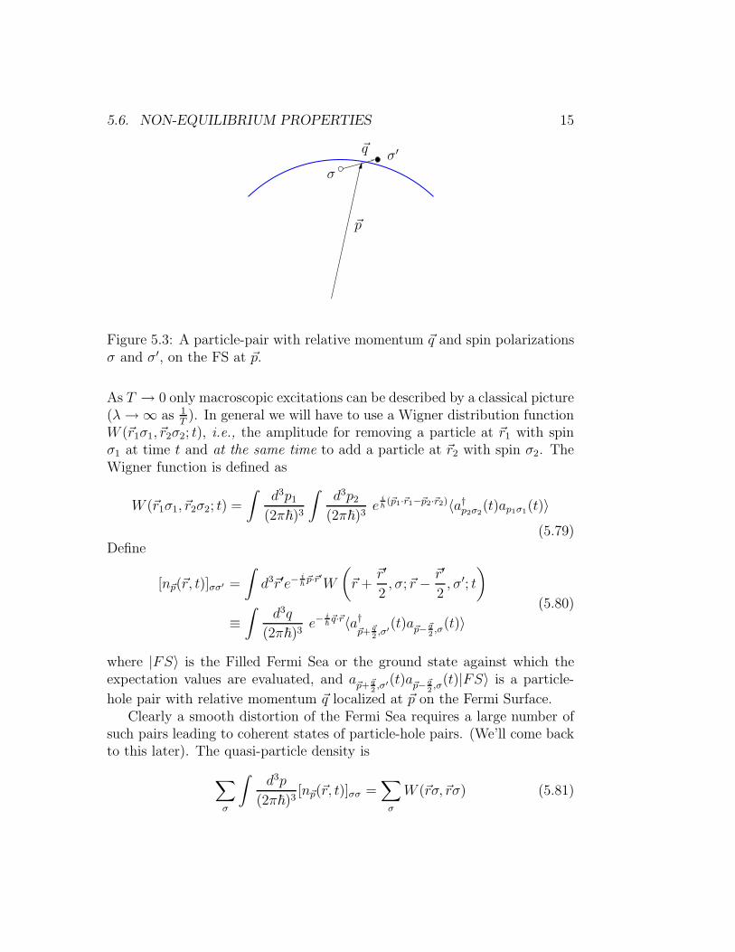
~p

~q

σ

σ′

Figure 5.3: A particle-pair with relative momentum ~q and spin polarizationsσ and σ′, on the FS at ~p.

As T → 0 only macroscopic excitations can be described by a classical picture(λ → ∞ as 1

T). In general we will have to use a Wigner distribution function

W (~r1σ1, ~r2σ2; t), i.e., the amplitude for removing a particle at ~r1 with spinσ1 at time t and at the same time to add a particle at ~r2 with spin σ2. TheWigner function is defined as

W (~r1σ1, ~r2σ2; t) =

∫d3p1

(2π~)3

∫d3p2

(2π~)3e

i~(~p1·~r1−~p2·~r2)〈a†

p2σ2(t)ap1σ1(t)〉

(5.79)Define

[n~p(~r, t)]σσ′ =

∫

d3~r′e−i~

~p·~r′W

(

~r +~r′

2, σ;~r −

~r′

2, σ′; t

)

≡

∫d3q

(2π~)3e−

i~~q·~r〈a†

~p+ ~q2,σ′

(t)a~p− ~q2,σ(t)〉

(5.80)

where |FS〉 is the Filled Fermi Sea or the ground state against which theexpectation values are evaluated, and a~p+ ~q

2,σ′(t)a~p− ~q

2,σ(t)|FS〉 is a particle-

hole pair with relative momentum ~q localized at ~p on the Fermi Surface.Clearly a smooth distortion of the Fermi Sea requires a large number of

such pairs leading to coherent states of particle-hole pairs. (We’ll come backto this later). The quasi-particle density is

∑

σ

∫d3p

(2π~)3[n~p(~r, t)]σσ =

∑

σ

W (~rσ,~rσ) (5.81)


and the number of quasi-particles with momentum ~p is

∑

σ

∫

d3r[np(~r, t)]σσ =∑

σ

∫

d3r1

∫

d3r2 e−i~p·~r1−~r2

~ W (~r1σ,~r2σ). (5.82)

For λ ≫ ~vF

kBT, note that [np(r, t)]σσ′ becomes a classical distribution.

If the system is inhomogeneous, the total energy E(t) may vary with time.We can still define εσ~p(~r, t) as the quasiparticle energy at position ~r

δE(t) =

∫

d3rδE(~r, t) =∑

σ

∫

d3r

∫d3p

(2π~)3E~pσ(~r, t)δnpσ(r, t) (5.83)

where δE(~r, t) is the local energy density. We have

δE~pσ(~r, t) =∑

σ′

∫

d3r′∫

d3p′

(2π~)3f~pσ,~p′σ′(~r, ~r′, t)δn~p′σ′(~r′, t) (5.84)

If the system is neutral the interactions are typically (assumed to be!)short-ranged and vary only over microscopic scales of the order of ~

pF. There-

fore, we can replace f~pσ,~p′σ′(~r, ~r′, t) by a local form. If there are Coulombforces

f~pσ,~p′σ′(~r, ~r′, t) ≈e2

|r − r′|δ(t − t′) + f~pσ,~p′σ′δ(r − r′) (5.85)

However many of these assumptions (concerning the existence and stabilityof quasiparticles) fails for transverse interactions (mediated by gauge fields)and in one-dimension. We will come back to this problem later.

5.7 Kinetic Equation

We now turn to the problem of the evolution (i.e. dynamics) of the quasi-particle disturbances. We will use Landau’s “quantum” kinetic theory. Webegin by looking at the regime in which δn~pσ(~r, t) can be regarded as aclassical distribution where it should obey a kinetic equation, i.e. the Boltz-mann equation. As usual this equation is simply the continuity equationfor δ~n~p,σ(~r, t) and embodies the condition of local charge conservation in thefluid. In the absence of collisions between quasiparticles their number mustbe constant. Hence,

d

dtδnσ~p(~r, t) = 0 (5.86)

5.7. KINETIC EQUATION 17

This implies that

∂

∂tδn~p(~r, t) +

∂

∂~r· (~v~pδn~p(~r, t)) +

∂

∂~p· (~f~p(~r, t)δn~p(r, t)) = 0 (5.87)

The quasiparticle group velocity in space is

~v~p(~nt) =∂

∂~pε~p(~r, t) (5.88)

The rate of change of quasiparticle momentum (the force) is

~f~p(~r, t) = −∂

∂~rε~p(~r, t) ≡

d~p

dt(5.89)

Hence we obtain Landau’s kinetic equation

∂

∂tδn~p − ε~p, δn~pPB = I[δnp′] (5.90)

where I[δnp′] is the collision integral, and PB denotes the Poisson bracket

εp, δnpPB =∂

∂~rεp ·

∂

∂~pδnp −

∂εp

∂~p·∂δn~p

∂~r(5.91)

Landau’s kinetic equation differs from the Boltzmann equation in that

1. εp can be a function of ~r, t

2. ∂∂~r

ε~p includes effective field contributions.

For example, if the system interacts with an external probe of the form of apotential U(~r, t), then the total energy is increased by

∫d~r · U(~r, t)δn(~r, t).

Therefore

∂

∂~rεp(~r, t) =

∂

∂~rU(~r, t) +

∫d3p′

(2π~)3f~p~p′

∂

∂~rδn~p′(r, t). (5.92)

The first term on the right hand side in the above equation is present indilute gases, wheras the second term arises from self-consistency conditionas effects of other quasiparticles.

In the quantum case one needs to use Wigner functions, giving rise to thequantum mechanical version of the kinetic equation. In Landau’s approach


one replaces the Poisson Brackets by 1i~

multiplied by commutators, pro-ducing the quantum mechanical equations of motion (see Baym and Pethick,pages 19-20). Near equilibrium we can linearize the transport equation, whichthen becomes the Landau-Silin Equation

∂δnp

∂t+ v~p ·

∂

∂~r

(

δnp −∂n0

p

∂εδεp

)

= I[np′] (5.93)

where ~vp and∂n0

p

∂εpare equilibrium functions. The Fourier transformed equa-

tion is

(ω − ~q · ~vp)δn~p(~q, ω) − ~q · ~vp

∂n0p

∂εp

δεp(~q, ω) = iI[np′] (5.94)

5.8 Conservation Laws

Let us first define

n(r, t) ≡∑

σ

∫d3p

(2π~)3n~pσ(~r, t) (5.95)

By integrating the Landau equation over ~p (and σ) we get

∂

∂t

(∑

σ

∫

p

npσ

)

+∂

∂~r·

(∫

p

∑

σ

~vpnpσ

)

+

∫

p

∑

σ

∂

∂~p(~fpnp) =

∑

σ

∫

p

Ip[np]

(5.96)

The number of quasiparticles is conserved upon collisions, therefore

∑

σ

∫

p

I[np] = 0

∫

p

∂

∂p· [fpnp] = 0

(5.97)

Let us define the current ~j(r, t) ≡∑

σ

∫

~p~vpn~pσ. The continuity equation,

which is just charge conservation, is

∂n(~r, t)

∂t+ ~∇ ·~j(~r, t) = 0 (5.98)

where~j =

∑

σ

∫

p

~v~p n~pσ =∑

σ

∫

p

∇~p εpσ(r, t)n~pσ(r, t) (5.99)

5.8. CONSERVATION LAWS 19

On linearizing around equilibrium we get an expression for the current density(superscript zero denotes equilibrium quantities)

~j =∑

σ

∫

p

(∇pε0pσ δnσp + ∇pδεpn

0p) (5.100)

Since

δnpσ = δnpσ −∂n0

pσ

∂εpσ

δεpσ (5.101)

which allows us to write the current as

~j =∑

σ

∫

p

[

~∇pε0pσ δnpσ − ~∇pn

0p δεp

]

(5.102)

Using that

~∇pn0pσ =

∂n0pσ

∂εpσ

~∇pε0pσ (5.103)

the current now becomes

~j =∑

σ

∫

p

(~∇pε0pσ)δnpσ (5.104)

Similarly we can write

δεpσ =∑

σ

∫

p′fpσ,p′σ′ δnp′σ′(r, t) (5.105)

δnpσ = δnpσ −∂n0

pσ

∂εpσ

∑

σ′

∫

p′fpσ,p′σ′δnp′σ′ (5.106)

I’ll keep only the Fermi surface contribution, and find that the current takesthe form

~j(r, t) =∑

σ

∫

p

(~∇pε0p)δn ~pσ(~r, t)

(

1 +1

3F

(S)1

)

=

(1 + 1

3F S

1

m∗

)∑

σ

∫

p

~p δn~pσ(r, t)

(5.107)

Galilean invariance implies 1 + 13

F(S)1 = m∗

m. Hence we have

~j =1

m

∑

σ

∫

p

~pδn~pσ =~P

m(5.108)


where the last ratio is momentum density over the bare mass. Otherwise,the general result is

~j =

(1 + 1

3F S

1

m∗

)

~P (5.109)

5.8.1 Momentum Conservation

The local momentum density ~g(~r, t) is given by

~g(r, t) =∑

σ

∫

p

~pn~pσ(r, t) (5.110)

It obeys the local conservation law

∂~gi

∂t+ ∇jTij +

∑

σ

∫

p

∂εpσ

∂rinpσ = 0 (5.111)

where

Tij =∑

σ

∫

p

pi∂εpσ

∂pjnpσ (5.112)

is (almost!) the stress tensor of the Fermi fluid. Using that

∂εpσ

∂ri

npσ =∂

∂ri

(εpσnpσ) − εpσ∂npσ

∂ri

(5.113)

and∑

σ

∫

p

εpσ∂npσ

∂ri=

∂

∂riE − n(~r, t)∇iU(~r, t) (5.114)

we can define the stress tensor Πij

Πij = Tij + δij

(∑

σ

∫

p

εpσnpσ − E

)

(5.115)

which implies that

∂gi(~r, t)

∂t+ ∇jΠij(~r, t) + n(~r, t)∇iU(~r, t) = 0 (5.116)

5.9. COLLECTIVE MODES: ZERO SOUND 21

5.8.2 Energy Conservation

Multiplying by εpσ and∑

σ

∫

pwe obtain

∑

σ

∫

p

εpσ∂npσ

∂t+ ~∇ ·

∑

σ

∫

p

(∇pεpσ) εpσnpσ = 0 (5.117)

We can now define the energy current density

~jE =∑

σ

∫

p

(∇pεpσ)(εpσ − U)npσ (5.118)

which obeys the energy conservation equation

∂

∂t(E − Un) + ~∇ ·~jE = −~j · ~∇U (5.119)

5.9 Collective modes: Zero sound

We will now look at the solutions of the Landau-Silin kinetic equation,Eq.(5.91), in the limit T → 0 in which the collision integral can be neglected.By linearizing this equation we obtain

(∂

∂t+ ~vp · ~∇

)

δnp(r, t) −∂n0

p

∂εp

~vp · ~∇δεp(r, t) = 0 (5.120)

with

δεp(r, t) = U(r, t) +

∫

p′fpp′δnp′(r, t) (5.121)

We now go to its Fourier transform and assume that the external potentialis monocromatic

U(r, t) ≡ Uei(~q·~r−ωt) (5.122)

and

δnp(r, t) = δnp(q, ω)ei(~q·~r−ωt) (5.123)

we obtain

(ω − ~q · ~vp)δnp +∂n0

p

∂εp

~q · ~vp(U +

∫

p′fpp′δnp′) = 0 (5.124)


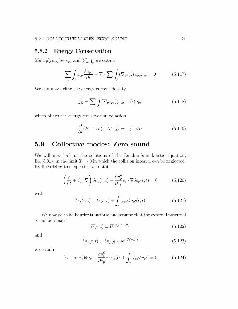
~p

~qθ

Figure 5.4: A particle-hole fluctuation with momentum propagating with ~qnear a point ~p on the Fermi surface.

Let us write δnp in terms of νp defined by

δnp ≡ −∂n0

p

∂εp

νp (5.125)

where we have assumed that only the Fermi surface matters. Within thisnotation we find that the linearized kinetic equation takes the form

ν~p +~q · ~v~p

ω − ~q · ~v~p

∫

~p′f(~p, ~p′)

∂n0~p′

∂ε~p′ν~p′ =

~q · ~v~p

ω − ~q · ~vpU (5.126)

with ~p on the Fermi surface.We will now make use of the azimuthal symmetry to expand the fluctu-

ation in partial waves

ν~p =

∞∑

ℓ=0

νℓPℓ(cos θ) (5.127)

and write∫

p′f(~p, ~p′)

∂n0~p′

∂ε~p′ν~p′ = −

∞∑

ℓ=0

1

2ℓ + 1F

(S)ℓ Pℓ(cos θ)νℓ (5.128)

Let us now define the dimensionless parameter s

s =ω

qvF(5.129)

5.9. COLLECTIVE MODES: ZERO SOUND 23

and

Ωℓℓ′(s) = Ωℓ′ℓ(s) =1

2

∫ 1

−1

dxPℓ(x)x

x − sPℓ′(x) (5.130)

The Landau-Silin Equation now takes the form

νℓ

2ℓ + 1+

∞∑

ℓ′=0

Ωℓℓ′(s)Fsℓ′

νℓ′

2ℓ′ + 1= −Ωℓ0(s)U (5.131)

This equation has solutions of the form νℓ(s).Let us consider first the s-wave channel, ℓ = 0. In this channel we find

Ω00(s) = 1 +s

2ln(s − 1

s + 1

)

= 1 +s

2ln∣∣∣s − 1

s + 1

∣∣∣+ i

π

2s θ(1 − |s|) (5.132)

and similar expressions in the other channels.For example, if we assume that the only non-vanishing Landau parameter

is in the s-wave channel, F s0 6= 0 and F

(s)ℓ = 0(ℓ ≥ 1), we find the simple

equationν0(s) + Ω00(s)F

(s)0 ν0(s) = −Ω00(s)U (5.133)

whose solution is

ν0(s) = −Ω00(s)U

1 + F(s)0 Ω00

(5.134)

The equation for the other angular momentum modes, with ℓ ≥ 1, is

νℓ

2ℓ + 1+ Ωℓ0(s)F

(s)0 ν0 = −Ωℓ0(s)U (5.135)

νℓ

2ℓ + 1−

Ωℓ0F0(s)Ω(s)00 U

1 + F s0 Ω00(s)

= −Ωℓ0(s)U (5.136)

νℓ

2ℓ + 1=

Ω(s)ℓ0 U [

F(s)0 Ω00(s) − 1 −

F(s)0 Ω00(s)]

1 + F(s)0 Ω00(s)

(5.137)

Hence,νℓ

2ℓ + 1=

Ωℓ0(s)

Ω00(s)ν0(s) (5.138)

The equation

ν0(s) = −Ω00(s)U

1 + F s0 Ω00(s)

(5.139)


ω

~q

zero sound

qvF

particle-hole continuum

Figure 5.5: Spectrum of collective modes

has poles at the zeros, s0, of

1 + F s0 Ω00(s0) = 0 (5.140)

We have the following regimes

• For 0 ≤ s < 1, Ω00(s) is complex. This solution corresponds to theparticle-hole continuum.

• For 1 ≤ s < ∞, Ω00(s) is a real and monotonically increasing functionof s.

In particular, in the latter case we find that if F(S)0 > 0, then there is a simple

pole with s0 > 1

s0 =ω

|~q|vF=

1 + e− 1

F0 , for F0 ≪ 1√

F(s)0

3, for F0 ≫ 1

(5.141)

This solution corresponds to an (undamped) sound mode with dispersionω = |~q|vF s0 and a sound velocity c0 = vFs0. This collective mode is knownas zero sound. Notice that the edge of the particle-hole continuum is atω = qvF . (See Fig.5.5).

5.10 The Quasiparticle Lifetime

The Landau interactions can in principle give rise to a finite lifetime τ forthe quasiparticles. However, if the lifetime remains finite as ω → µ = EF ⇒

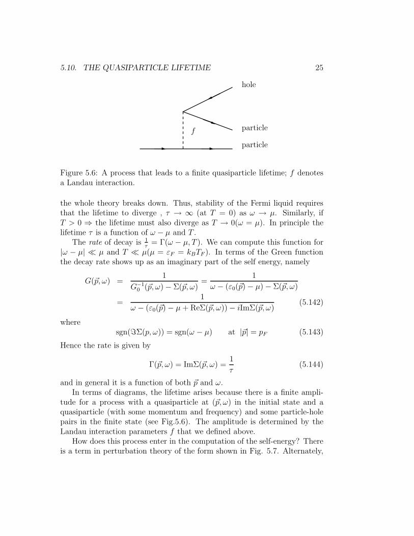
5.10. THE QUASIPARTICLE LIFETIME 25

particle

particle

hole

f

Figure 5.6: A process that leads to a finite quasiparticle lifetime; f denotesa Landau interaction.

the whole theory breaks down. Thus, stability of the Fermi liquid requiresthat the lifetime to diverge , τ → ∞ (at T = 0) as ω → µ. Similarly, ifT > 0 ⇒ the lifetime must also diverge as T → 0(ω = µ). In principle thelifetime τ is a function of ω − µ and T .

The rate of decay is 1τ

= Γ(ω − µ, T ). We can compute this function for|ω − µ| ≪ µ and T ≪ µ(µ = εF = kBTF ). In terms of the Green functionthe decay rate shows up as an imaginary part of the self energy, namely

G(~p, ω) =1

G−10 (~p, ω) − Σ(~p, ω)

=1

ω − (ε0(~p) − µ) − Σ(~p, ω)

=1

ω − (ε0(~p) − µ + ReΣ(~p, ω)) − iImΣ(~p, ω)(5.142)

wheresgn(ℑΣ(p, ω)) = sgn(ω − µ) at |~p| = pF (5.143)

Hence the rate is given by

Γ(~p, ω) = ImΣ(~p, ω) =1

τ(5.144)

and in general it is a function of both ~p and ω.In terms of diagrams, the lifetime arises because there is a finite ampli-

tude for a process with a quasiparticle at (~p, ω) in the initial state and aquasiparticle (with some momentum and frequency) and some particle-holepairs in the finite state (see Fig.5.6). The amplitude is determined by theLandau interaction parameters f that we defined above.

How does this process enter in the computation of the self-energy? Thereis a term in perturbation theory of the form shown in Fig. 5.7. Alternately,


Figure 5.7: Feynman diagram with a contribution to ImΣ.

the imaginary part comes from effects of the collision integral (see Baym andPethick p. 87) and is given in terms of the t-matrix:

1

τ~p=

∫d3q

(2π)3

∫d3p′

(2π)3

2π|〈p − q, p′ + q|t|p, p′〉|2δ(ε(p) + ε(p′) − ε(p − q) − ε(p′ − q))

×[n0(p′)(1 − n0(p′ + q))(1 − n0(p − q)) + (1 − n0(p′))n0(p′ + q)n0(p′ − q)]

(5.145)

which follows from using Fermi’s Golden Rule. The first term in the expres-sion in brackets in Eq.(5.143) represents the rate at which quasiparticles arescattered into new unoccupied states while the second term represents theblocking of such processes due to occupied states.

The t-matrix amplitude 〈p − q, p′ + q|t|p, p′〉 is represented by summingup particle-particle (or particle-hole) ladder diagrams, scattering processesof the type shown in Fig.5.8, given by the solution of the Bethe-salpeterEquation (see Baym and Pethick, p. 77):

t~p~p′(q, ω + iη) = fp,p′ −∑

p′′ 6=p′

fp′′,p′~q · ~∇p′′n

0p′′

ω + iη − ~q · ~vp′′tp′′p′(q, ω + iη) (5.146)

The matrix elements of the t-matrix can also be split into a singlet tS andtriplet tA channels, and further be expanded in angular momentum compo-nents, tS,A

ℓ :

tpp′(q, 0) =∑

ℓ

tℓ(q, 0)Pℓ(cos θ) (5.147)

5.10. THE QUASIPARTICLE LIFETIME 27

whose coefficients are given by

tSℓ =fS

ℓ

1 +F s

ℓ

2ℓ+1

|q| ≪ pF (5.148)

tAℓ =fA

ℓ

1 +F A

ℓ

2ℓ+1

|q| ≪ pF (5.149)

After some algebra on finds that the decay rate at finite temperature T andfrequency ε at zero momentum transfer (i.e. on the Fermi surface) is givenby

1

τp≈

π(N(0)t(0))2

8πvF (p2F /qc)

[(ε − µ)2 + (πkBT )2] + · · · (5.150)

(qc ∼ Λ is a momentum cutoff) which satisfies Landau’s assumptions.The Landau picture we discussed works very well in neutral Fermi fluids

(such as the normal phase of 3He) and in most (simple) metals. Howeverwe will see that it fails in a number of important situations. In particular itfails in one dimension (for any value of the interaction coupling constants)and also near a quantum phase transition. It also fails in systems with strongcorrelation.

Figure 5.8: Feynman diagram that contributes to t~p~p′(q, ω+ iη) in the Bethe-Salpeter Equation (5.144).

chapter 5 landau theory of the fermi liquideduardo.physics.illinois.edu/phys561/fl.pdf · chapter 5...

Documents