chapter 6 figures - nrc

Chapter 6 Figures

Waste Form Degradation, .Radlonuclide Mobilization, .:and Transport through the

Engineered System * Radionuclide inventory * Spent Nuclear Fuel (SNF) dissolution

, Solubilities * Colloid formation * Cladding failure

* High Level Waste (HLW) dissolution

* Secondary phases F Flow and dissolution

Waste Form •Radionuclides Mobilized

"Temperature Inputs Outputs Aqueous Radionuclide Outputs Concentration

Water Entering

Waste Package Colloid Fraction

(quantity/chemistry) ....

, Waste Inventtory * U0 2 dissolution tests

* SNF dissolution tests * HLW dissolution tests

SLiterature cladding failure * Solubility tests

* Expert elicitation * Natural analogs

V1&-.,*d Cofdec ** S S. *A,

Figure 6-1. Waste form degradation, radionuclide mobilization and transport through the engineered

barrier system.

August 1998BOOOOOOOO-01717-4301-00006 REVOO F6-1

(

0>

0D

0 6

0n

C)

a

.0

- - - - - - - - - - - - - -

I - - - -- - - - - - - - - -

- -- - - - - - - - - - - - -

- - - - - - - - - -

CD

3D 0)

0l.

4-

I--

I I

.0

I -41

I I .0 I -�,

I -� Ii

0 1

- - - - - -

L -I - - - - - - - -B b

0)

.0

(

* Y .0

C)

-do-

�11 0'

.0

'D

0L r_

U)

'D

-~ I

C) IM

-0

- -- - - - -- -a4 ---- ----

Cladding Failure

Local Mechanical Splitting corrosion disr ption

Water seepage

Air-steam environment

Waste Package Cross-Section

Fuel Assembly

SAdsorbed Water

SRadionuclide Inventory

* Gap and grain boundary V U0 2 matrix * Secondary phases

Transport Pathways

Y Diffusive Y Advective x

Single Fuel Element with Claddiný

Fuel Degradation and Pellet fragmentation Radionuclide Mobilization

Secondary phase formation Adsorbed water (porous and water saturated)

Grain boundary U02m,

Figure 6-3. Schematic of waste form/waste package/engineering barrier system.

B00000000-01717-4301-00006 REV00 F6-3 August 1998

T(t),qwp(t),RH(t) -----------------

Thermo- # pits( Wasi hydrology Degr

T(t) qwf(t)

- - - - -- - - - - - - - - - - -

failed(t)

Cladding - Failures - Unzipping

Fuel surface area exposed(t)

---------------L-----------

i

L ---------------------------------Ir T -I

L---------- ---- ------

, Radionuclides available(t)

-------------- - --------

Solubility models: Colloid Calculated/ formation as observed

Dissolved RNs Colloidal RNs mobilized (t) mobilized (t)

To EBS Transport1! 'V

Figure 6-4. CSNF degradation/radionuclide mobilization process flow.

B00000000-0 1717-4301-00006 REVO0

C(t)

- -- j - - - - -

F6-4 August 1998

Stainless steel and juvenile failures

Failed at emplacement -2

)-3

)-4

.-5-....................

104 105 Time (years since WP failure)


106

106

100

C Zirca CU 5 10.1

LL 2 10-2

S10.3

L 10-4

C)

10-s 103

Figure 6-5. TSPA-VA cladding abstracti


B00000000-01717-4301-00006 REVOO

C 0 C.)

LL

LL

CM

"*0 CU "U

10

10

10

1C

10

10103

100C 0

o5

LL

CU 5.

LL

"L.

"0) C Vo

10-1

10-2

10-3

10-4-

FMechanical failure]

Upper

Lim'

Lower limit

1-5 01 10Q3

106

August 1998F6-5

1201 ABS-CE PWRs

LEAST SQUARES FIT LINE SHOWN

100 0

0 60

z 00

z9 0 0

60

wESTIMATED nVa Uj ~~TRANSITION 0- i

0 40-8 G a

20

0CO 20 40 60

BURNUP. MWd~kg

Figure 6-6. Cladding oxide thickness vs. bumup.

From: A.M. Garde, "Enhancement of Aqueous Corrosion of Zircaloy-4 due ot Hydride Precipitation at Metal-Oxide Interface," ASTM STP 1132,1991, p. 583.

130000O000-0 1717-4301-00006 REVOO F- uut19August 1998F6-6

1500 M4

8400 £

g300-.. ,\(•

•200

I00

0

0 30 40 so 60 70

FUEL ROD BURNUPI (GWd/TU)

Figure 6-7. Total hydrogen content for cladding vs. bumup.

From J. P. Mardon, et al., "Update on the Development of Advanced Zirconium Alloys for PWR Rod Claddings," ANS Proceedings, 1997 Topical meeting on LWR Fuel Performance, Portland, OR, March 26, 1997, p. 408.

B00000000-0 1717-4301-00006 REVOO F6-7 August 1998

C a 1.0

... Plenum

C 0.8 £1 & Peak oxide C U 0

S0.2

* 0,4

z 0o0

0 100 200 300 400 S00 600 Distance from clad o.d. (grm)

Figure 6-8. Cladding radial hydrogen profiles.

From: D.I. Schrire, ,4.H. Pearce, "Scanning Electron Micropscope Techniques for Studying Zircaloy Corrosion and Hydriding," Zirconium in the Nuclear Industry: Tenth International Symposium, ASTM STP 1245, A.M. Garde and E.R. Bradley, Eds, American Society for Testing and Materials, Philadelphia, 1994, pp. 98-115.

B00000000-01717-4301-00006 REV00 August 1998F6-8

0 10 20 30 40 50 60 MWdIkgU 80

Rod Average Bumup

Figure 6-9. Fractional fission gas release for PWR fuel as a function of bumup.

From: R. Manzel, M. Coquerelle, "Fission Gas Release and Pellet Structure at Extended Bumup," ANS Proceedings, 1997 International Topical Meeting on LWR Fuel Performance, Portland, OR, March 2-6, 1997, pp. 465.

BOOOOOOOO-01717-4301-00006 REVO0 August 1998F6-9

Center Pin Temperature vs Time

a)

E a) E I

I-.

350

300

250

200

150

100

50

010 100 1,000 10,000

Time from Repository Closure (Years)

Figure 6-10. Center pin temperature vs. time.

BOOOOOOOO-0 1717-4301-00006 REV0O August 1998F6-10

1.000) - - Outer Barrier "cc Inner Barrier LL. _ 1st Breach

0 1st Pit �.lst Patch

0.50 0 /

0 0.25 Co) *6 /

.. NEa5.et.jt / J u_ 0.00

102 103 104 105 106

Time (years)

Figure 6-11. Base case waste package failure.

B00000000-01717-4301-00006 REVOO August 1998F6-1 1

"• " 10-2 .C-22 .. .. •..........

,E0 5 0 •percentle S10-3 .C-22-110 50 .•

C 10-5 • C.22'.OOo -50

on -6

o0 106 . L..

0 ~ 01ets 0

10-8 .

20 40 60 80 100

T (°C)

Figure 6-12. WAPDEG corrosion rate used for cladding corrosion.

B00000000-0 1717-4301-00006 REVOO August 1998F6-12

100

10-1

10-2

10-3

10-4

10-5.

10-6.

- -C.

-22 Rate/lO -22 Rate/100 -22 Rate/1000

I //

I ! II. *1

102 103 104 105 106

Time (years) from the I st Waste Package Breach

Figure 6-13. Fraction of fuel exposed from zircaloy clad corrosion.

B00000000-01717-4301-00006 REV0O

V)

0~

'I-

F6-13 August 1998

102. U) .- 1 1 .. / . ..

0) Peehs

o 100

S10" Matsuo 103

*j10-2

200 250 300 350 400 450

Temperature, °C (Constant during 10 years)

Figure 6-14. Comparison of creep correlations at constant temperature.

B00000000-01717-4301-00006 REVOO F6-14 August 1998

(.

Fracture Toughness, MPa V/m

0 -0

o o oo•

CL

0 0

o0 . .. .. ... - , ,

CD o t o

000

o -o

_NU. .~

0 )

-@ "

>C

oCD

15 khichcgfa

0

5"".............. 7,

------ hydride thickness = 2 gm

- hydride thickness 3 irm experimental data

40 50 60. 70 H in solution (C.) (wt ppm)

Figure 6-16. KIH as a function of hydrogen in solution. Lines: theory predictions from Shi and Puls, 1996.

B00000000-0 1717-4301-00006 REVOO August 1998F6-16

380 - 30+ . 360 ,• % 100%. " 340- Reorientation" .. 100%

v 320 V

300 . No Reodrentation

S280

E 260 0 Marshall I- 240 - v Einziger

220 - Hardie minimum a 2 PULS

200 120 140 160 180 200 220

Stress (MPa)

Figure 6-17. Temperature and Stress at which Hydrogen Reorientation was Observed for Cold Worked

Zirc-2, 4 [Pescatore, et a/, 1989]

B00000000-01717-4301-00006 REVO0 F6-17 August 1998

5

C)

0 U-

4

3

2

1

0 vI I I I

0 1 2 3 4 5

Displacement

Figure 6-18. A comparison of the empirical equation, Equations 6-10 and 6-11, and the exact treatment for the force-displacement relationship using standard elastic-plastic beam theory (see text).

BOOOOOOOO-01717-4301-00006 REVOO August 1998F6-18

Figure 6-19. A sketch of the simplified conceptual model of the mechanical damage process. Due to ultimate failure of a waste package, a rock block falls on the center of an assembly of rods, which is modeled as a continuum in its force-displacement and energy absorption behavior. The shape of the block is idealized later. The distribution of possible block sizes is discussed in the text.

B00000000-01717-4301-00006 REVOO F6-19 August 1998

Figure 6-20. Schematized geometry of a block and its impact. The axes of the blocks are taken to be vertical, and the blocks are assumed to fall freely from the former waste package surface onto the fuel assemblies. See Fig. 6-21 for more detail on the punch shapes.

B00000000-0 1717-4301-00006 REVO0 F6-20 August 1998

LI Crcular Punch Linear Punch

Figure 6-21. Two types of punches are considered. For a circular punch, the focusing parameter is the ratio of the diameter of the punch to the diameter of the block. In a linear punch, two parallel chords of equal length and the two block-edge arcs that connect them define the outline of the punch. The focusing parameter is then defined as the ratio of the distance between the two chords to the diameter of the block.

B00000000-0 1717-4301-00006 REV00 August 1998F6-21

Clad Unzipping (U308 formation) vs. Waste Package Failure Time

100

80

60

40

20

0

10 100 1000

Waste Package Failure Time, Yrs.

10000

Figure 6-22. Clad unzipping vs. waste package failure time.

B00000000-0 1717-4301-00006 REV00

tCL

t-

CL

a.

0

0) 10. 0i 0

F6-22 August 1998

104

183

z 760 26

So2- 760. 1

o 26277/'

0/ ---- BARE ROD END / FUEL FRAGMENTS

I

10 / - BARE ROD CENTER /' ,FUEL FRAGMENTS

/ o 760 Am--ROD CENTER 0 760 Mm- ROD END O <50 Am -ROD CENTER * <50 Mm--ROD END

1,1 1

15 16 17 18 19 20 21 22

1IT (K x 104

Figure 6-23. Time-to-cladding-splitting (in hours) from Einziger and Strain (1986), with a more general proposed fit added (the longer, lesser-slope line). The new fit uses a Q value from other experiments, and is a best-estimate fit to both rod-end and rod-center data combined. The original fits (shorter lines) were intended to be lower-bound fits for the data sets, treating rod-end and rod-center data groups separately.

BOOOOOOOO-01717-4301-00006 REVOO F6-23 August 1998

Figure 6-24. Comparison of the input data with the fitted function, for log of rate, for all the spent fuel and U0 2 data.


(left) Vary together: T,02@BU=30; (right) Vary C03@BU=30

2.00

1.50

1.00

0.50

0.00

-0.50 -

* PredictU.Diss.

- Err. w/o residual

- Err. w/o residual

-1.00

sequence in variation

I I I I I i l I I l l l l l l l l l l l l l l l l l lI I t I I I

LO~ M4C M~ I* Mr

Figure 6-25. Error bars for two typical data series through the span of data covered by the fitting data and extending beyond the fitting data; errors in the coefficients, i.e., fitting errors, only. On the left: increasing temperature, range 5 to 950C (experimental range 25 to 750C); increasing 02, range 0.1% to 40% with a logarithmic spacing of intermediate values (experimental range 0.3% to 20%); bumup = 30 MWdays/kgU; other parameters near their logarithmic averages for the data set, specifically pH = 9, CO3 = 2 mmol/l. On the right: increasing C03, range 0.05 to 80 mmol/1 % with a logarithmic spacing of intermediate values (experimental range 0.2 to 20 mmol/I); bumup = 30 MW-days/kgU; other parameters near their logarithmic averages for the data set, specifically T = 500C, pH = 9, 02 = 2%.

BOOOOOOOO-01717-4301-00006 REVOO

0

4.0

0

l l l l l l l l l l l l l l l l l l l l l l l l l l.l.ll l l l.lll l l l

August 1998F6-25

Figure 6-26. Error bars for two typical data series through the span of data covered by the fitting data and extending beyond the fitting data; same data series as in Fig. 6-25; fitting errors and residual error are included.

B00000000-01717-4301-00006 REV00

(left) Vary together: T,02@BU30;(left) Vary together: T,O2@BU=30;

(right) Vary C03@BU=30

2.00

1.50

S1.00

oi 0• PredictU.Diss. S0.50 - Er;. w. residual 0 - Err. w. residual

0.00

-0.50

-1 .00in iaion

sequence in variation

F6-26 August 1998

Linear (U diss rate) for 3 interpolations

Figure 6-27. Different logarithmic interpolations from end points based on the low-end and the 30 MWdays/kgU points of Equation 6-27. We vary the lower end x-value and keep the upper x-value of 30 MWdays/kgU. The difference is seen to be small for the higher bumup values within this bumup range.

BOOOOOOOO-0 1717-4301-00006 REVOO

4.50

4.00

3.50

3.00

2.50 "I--'- Interp

2.00 I. Iter

1.50

1.00

0.50

0.001

0 5 10 15 20 25 30

Burnup

F6-27 August 1998

Comparison of Dissolution Rates for Different Waste Types 1E+5

1 E+4 -

1IE+3 - -- -

"" 1E+1

Q 1E-1 - - - -

I E-2

"•• 1 E-3 . . . . . . . . . . . . . . . . . .. .

"0 Waste Types S1E-4 1E�-� Oxide Spent Fuel

1 E-5 . . . . . . . .. . . . . - 4 - L

1E-6 . .Metallic Spent Fuel

-,-- Ceramic Spent Fuel

E-•-- Carbide Spent Fuel

1 E-8 4--- - -- I

0 20000 40000 60000 80000 100000 120000 Time (years)

Figure 6-28. Comparison of dissolution rates for HLW, metallic spent fuel, oxide spent fuel, carbide spent

fuel, and ceramic spent fuel.


gel layer 4 /, diffusion la er

Ssecondary phases

Si

Glass begins to react with water

Hydration and ion exchange of the surface.

Diffusion layer thickens until rate of diffusion of alkalis equals rate of network dissolution.

Diffusion layer maintain constant thickness as glass dissolves at steady state. Secondary phases continue to grow.

Figure 6-29. Glass dissolution mechanism (from Bourcier 1994).

BOOOOOOOO-0 1717-4301-00006 REVOO F6-29 August 1998

200 Li 1 6 ... ... .. ... ..... ......... ..... .. .... .. .... ... ... ........... ......... .........

z 0 . ... .. .. .... .....'... . ... ... .... . .... ......' .. .. ..... ... .... ... ....-J .. .... ...

8 0 . ..... ... ......... .......... .. ... .................. .t .............. ............. .. .............. .

1 0 1T**

0- .5 1 1.5 2 2.5 3

Time (days)

Figure 6-30. Normalized elemental release from SRL-165 glass reacted in 0.003M NaHCO3 at 1500C, SAN 0.01cm"1.

B00000000-01717-4301-00006 REVOO F6-30 August 1998

2 I

logiok = -1.5775 - 0.6381(pH-3.19) -2991.7706(1 I(T+273.15) --0.003109)

A* T = 70'C

0 Q , A

ca -1 --, 'AO "i'" /O E 250 S-2

o ~\ 0

-4

-5 Ioglok =-2.4138+ 0.4721 (pH-9)-4502.9765( 1/(T+273.15) -0.003109)

"-6 I .I I I I I I - I 1 .

0 2 4 6 8 10 12 14 pH

Figure 6-31. Loglo(dissolution rate, g/m2/day) versus solution pH.

B00000000-0 1717-4301-00006 REVOO F6-31 August 1998

lu

C)

CU

LW

25

20

15

10

5

0 L0.1 1 10 100 1000 10o4

COOLING RATE°/HR

Figure 6-32. Area increase of thermally shocked simulated nuclear waste glass. Values are relative to geometric area of glass cylinder with no surface roughness. Data from Ross and Mendel 1979.


Comparison of Np Values

20 40 60 80

Temperature, °C

4-1

-2

-3

-4

-5

-6

-7

-8

100

Oversaturation Study

Nitsche et al., 1993 (pH=5.9)

Nitsche et al., 1993 (pH=7.0)

ANitsche et al., 1993 (pH=8.5)

Dissolution Studies

3

0)

CF

0 0 0, -20

-3

-4

Figure 6-33. Range of revised solubility-limited Np concentration distribution (shading) for TSPA-VA (after Figure 3-1 M&O, 1998). Comparison of the previous range of project elicited values (bar) based on the oversaturation measurements of Nitsche et al. (1993) with the values derived from spent fuel dissolution studies starting from undersaturation and the range of the revised (shading) distribution (st. st. = steady state; avg. = average of whole test time for Finn et al., 1995 study).

B00000000-0 1717-4301-00006 REVOO

on, 1995

95 (avg. 106)

95 (avg. 103)

95 (st. st. 106 ) 95 (st. st. 103 )

0 E3

Wilson, 1990a

Gray and Wils

Wilson, 1990b

Jardine, 1991

Finn et al., 19, IFinn et al., 19,

Finn et al., 19, V Finn et al., 19

C0

CU

0

0 0

-9

-10

F6-33 August 1998

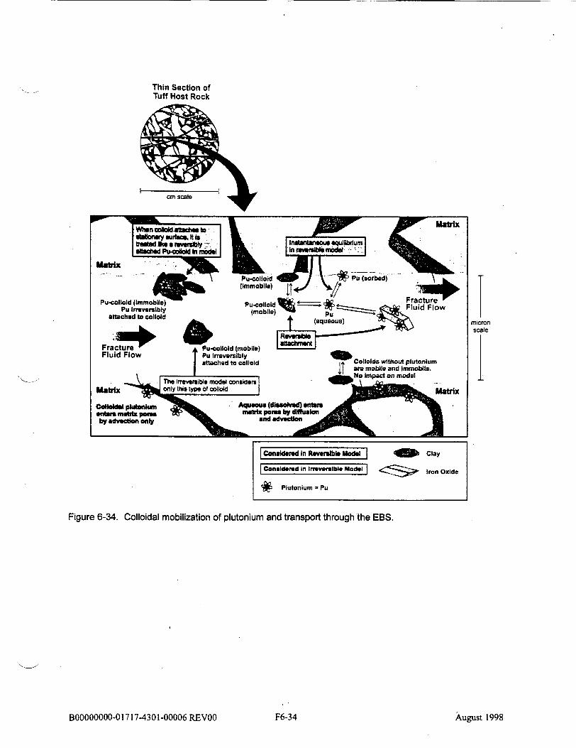
Thin Section of Tuff Host Rock

1scaleicon

Figure 6-34. Colloidal mobilization of plutonium and transport through the EBS.

B00000000-01717-4301-00006 REVOO

Cwweder'd In Rowulble Model 41M Clay

Considered in ,ruverlbae Model I Iron Oxide

SPlutonium = Pu

F6-34 August 1998

. Drip WeUnaltered Spent Fuel S Li )

tar Alteration

Alteration Layers

Vapor Condensation

0• 0 0

00.

0) 0 0•

0

-4

0

OI

S . .VCondensed Vapor

+ Drip Water + Dissolved Solids

+ Mobilized Colloids

Experimental Test Configuration

S Channelized Drip Water

Condensed Vapor-Water

Fluid Flow Patterns in Spent Fuel Fragment Pile

Figure 6-35. Experimental test configuration.

(.

Water Vapor

ter

0

C> 0

CD ATM103: Fitted Film Mass Concentrations 0

S•" 1.0E-03

SE 1.OE-04 - Pu

S1.OE-05 U ' 1.OE-06 - CS

S1.OE-08 - Sr

0 1.OE-09 Mo S=I 1.0E-11 0.E-A

1.0E-12 1 -- Np

E 1.OE-13 2

0 200 400 600 800 1000 1200 1400

Time (days)

00

Figure 6-36. Equilibrium film mass concentrations fitted to ATM-103 spent fuel vapor test and low-drip test data using advective transport limited approximate model.

ATMI06: Fitted Film Mass Concentrations

•0 0 0

0

0.

"-3

0

O0

1.OE-03 1.OE-04

1.OE-05 1.OE-06

I.OE-07 I.OE-08 1.OE-09

I.0E-10 1.OE-1 I 1.OE-12 1.0E-13

1000 1200 1400

Figure 6-37. Equilibrium film mass concentrations fitted to ATM-106 spent fuel vapor test and low-drip test data using advective transport limited approximate model

(

0 200 400 600 800

Time (days)

LL

C 0

U C)

0E

-. U

--- Cs

-- Sr SMO

---Am

-e-Np

--. -I

Long-Term Film Concentrations Vs TSPA (1995) Solubilities

6

0 0 0 0 0 0 0 0

00

00

-T"

I.<

00U Cs Tc Am Np

Figure 6-38. Comparison of long-term equilibrium film mass concentrations fitted to spent fuel vapor test and low-drip test data against TSPA 1995 recommended solubility limits. Neptunium solubility limits have been reduced by two orders of magnitude in this analysis (TSPA-VA) from the values shown (Section 6.4.3.1.4).

(

Pu

-J E

Z,

0

0

M.)

1.0E+00 I.OE-01 1.OE-02 1.OE-03 1.OE-04 1.OE-05 I.OE-06 1.OE-07 1.OE-08 1.OE-09 I.OE-10 1.OE-I 1 1.OE-12 1.OE-13

" ATM-103 Film Concentration @ 925 days

" ATM-106 Film Concntration @ 926 days

1 TSPA 1995 - Solubility Minimum

I TSPA 1995- Solubility Average

E TSPA 1995- Solubility Maximum

Dripping Water

spent fuel 14%

steel + cladding 21 % (inactive)

porosity 65% 1.56 m

specific surface area 39.6 cm 2/g

Figure 6-39. Schematic of simulation configurations.


E E• (D CD

C-)

0~

CD

0

0.0

0.3

0.6

0.9

1.2

1.50 2e-12 4e-12 6e-12 8e-12 le-ll

Dissolution Rate of U0 2 (g/cm2-sec)

�I�

... ...... . .. ................. ........................................... ........ .. .. ...... .. . . . . . .

I I .........................................-....... ................ . .. .........

....... ..... I..

I I I - L ,I I I

0

..... ' ....................... I .../ ..

I

"• , ,1

1

-t = 0 year S- t=10

t-- t=100 --- t=200

•-t =500

2

U02 (vol.%)

Figure 6-40. Profiles of dissolution rate (a) and volume fractions (b) of spent fuel for Case A. The

dissolution rate varies less than 15% with time and space. Available spent fuel is totally consumed after 500 years of dissolution.


1i/ ...................... i

!.1 ........................i ......

S.......... " ............. . . .

S.............. •..........i ............ - - t = 2 0 t =0 year t= 10 t =t 100 ...

-~~ = - t200 I . .. t = 500

*I ....................... i .............................. .................................. .. .

• . .. . . . ... . . ... .. .. . .. . .... . . .. ... |

E

0) Ca

0C.,

a) 4-0 Cu

CU

3C

0

0.0

0.3

0.6

0.9

1.2

1.5

i i

I

August 1998F6-40

C.I

0

CO

C-C

U, 0

0.0

0.3

0.6

0.9

1.2

1.50 I 2 3 4 5

Schoepite (vol.%)

(a)

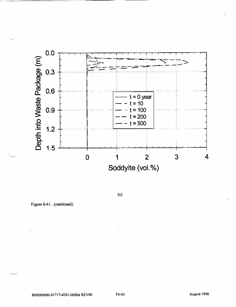
Figure 6-41. Volume profiles of secondary minerals precipitated when spent fuel dissolves. (a) schoepite, the major secondary minerals; (b) soddyite, precipitated at the top of WPs and re-dissolved after spent fuel is consumed; (c) uranophane, mainly precipitated at the top of WPs. Closely exam the movement of precipitation fronts reveals, though not very obvious, that the growth of uranophane is at the expense of schoepite and soddyite.

B00000000-0 1717-4301-00006 REV0O

. ............ ....... t - 0 g a.............. ............... . .. ... . .. .. .... ............ .. t=lO I I

t = 100 a . t = .2 0. ......0 ...... .... ......... .... ..... I. . ........ .. . ... ... ..... . .

t = 500 7 t =1,000 .I...... • • ................. ... .. ------ t....... ..... .i .... ................ .

-.... 1o......i,,, ... I i,,

August 1998F6-41

06OA3dI 90000-0 Et'-L I L 10-00000000O

(q)

(%'IOA) ueqdouwn

01, 9 9 0I I I I I I I I

000'1 : =I OO :=1 009 = I - --

UMb =41 O = I ............ ....... ...... .... .

JeeA 0 = I

.. . ...

• "• •LI I

9.0 CD

-0

-6"0 Z')

CD

-90"0 0

CD

-e'o a: CD

~0 3

I I I

. . ............. .... .......... ....

... ... .. . ... ..

. ......... .... .. ..

. ......... ..........

, , I

II I . .S. . . . . . 1 I

8661 jsn~nV

(panuiluo) -I1t-9 am•!Ij

0

0.0 0.3

0.6

0.9

1.2

1.5

(c)

Figure 6-41. (continued)


E a)

.)_

cc

cn CU

CL

I I

2

Soddyite (vol.%)

I ISI I I I I I I i

S. . . ... ... . . .... ........ ........ .................... ...... f . .................... .. ... .. . , .. .. .. ... ...... -. .. .. .. .. .. .

....................

- -- t yal

t=100 .. . t = l O00 ..... .. .

--- t=200 t = 500

2 .....

3

3 4

August 1998

I I

F6-43

Figure 6-42. Paragenetic sequence of secondary minerals observed in the simulation results. Dashed line means meta-stable phases. Uranophane is the most stable uranyl mineral.

8.20

8.15

8.10

8.05

8.00

7.95

7.90200 400 600 800

le-3

le4

le-5

le=6 le-7•

le-9

le-101,000

"Tnrm (yr.)

Figure 6-43. pH and U(total) concentration changes for Case A. pH drops from its original value of 8.2 to 7.95 at 10 years and then reverses to its original value. U(total) increases first and then decreases.


Spent Fuel

Schoepite

Soddyite

Uranophane

F6-44 August 1998

0.0 1 o.3 . .

, 0.6 - -\500 & -- 1..... .... 4 00

1,000

S0.9 - 10,000 I 1 -- 20,000 O - 50,000

i 1.2

1.5- ,> ,11. -,,

0 1 2 3 4 5

Schoepite (vol.%)

Figure 6-44. Simulated schoepite profiles for Case-1 at different time. Schoepite dissolves and disappears at 50,000 years. Before 10,000 years, the dissolution takes place across the whole WP. After that dissolution is localized to the dissolution front, which advances with time from upstream to down stream.


0.0h

0. 3

/.. .- 100 ~0.9 -I-0 500

-1,0C "1.2 I

0 2 4 6 8 10 12

Uranophane (vol.%)

Figure 6-45. Simulated uranophane profiles for Case-1. Uranophane replaces schoepite. Before 10,000 years, it precipitates across the whole WP. After that time, the precipitation front advances from upstream to downstream.

B00000000-01717-4301-00006 REVOO F6-46 August 1998

CU (.

Cn C

0

-C w~

0.0

0.3

0.6

0.9

1.2

1.5le-10 le-9 le-8 le-7 le-6 le-5

U concentration (mol/kg)

Figure 6-46. Simulated concentrations of U. It increases with depth into WP and reaches its maximum at the bottom of WP. After 50,000 years, U concentration at the bottom decreases.

B00000000-0 1717-4301-00006 REV0O

SI I Ir-T 10 11 1 1 It'l 1 -1 1 1 1 1

.. . ... . ........................... .............................. ... ...... ... ................ ..... . ..... .. .. ... . . . . . .. ,

t 0OyearNj ..... ................... ..... 1 0 0 ............. ......... .. .. .. .. .. .. . .. ... .... .. ... .... 500 I

... 1,000 S. .............................. . 3 ,0 0 0 . .

10,000 -... .20,000 S.... ......... ....... ........... ............ .............. ' , ..................... '..

500,000 I

1 e-4

F6-47 August 1998

1 -. .1P ... . .

le-14 le-13 le-12 le-ll le-10 le-9 le-8 le-7 le-6

Np(total) Concentration (mol/kg)

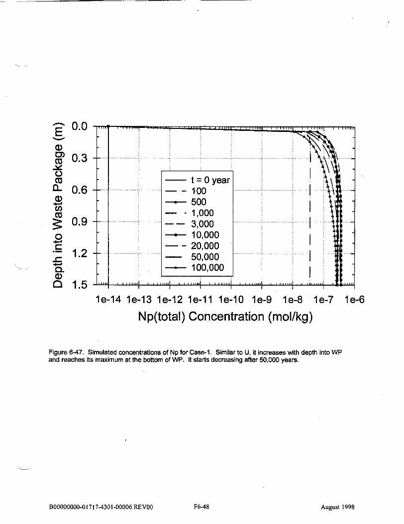
Figure 6-47. Simulated concentrations of Np for Case-1. Similar to U, it increases with depth into WP and reaches its maximum at the bottom of WP. It starts decreasing after 50,000 years.


0.0

0 .3 t ....

E a,

CO

CU

C.CU 30

0.6

0.9

1.2

1.5

t = 0 year --- 100

500 -- - 1,000

3,000 10,000

--- 20,000 50,000 100,000

.,,i

August 1998

I I I I I I i . .

I

.. ..... . . . .

S..................... i ... . ...

S. .... i . . ..I i i Iiiii

F6-48

C0

o

o

o - e-4

oE TSae CCase-I: 70°C, 11% C.F, H, SI e -5 ~ ~~~~~~...a se P............. ...... ....................... ...................................... ............... - - c a e 2 7 0 , 1 % C F , H l-e-5 BsCae- -Case 2: 70'C, 1% C. F., Hy

O g - - Case-3: 300C, 11% C.F., H § l e - - ;........................... .................. ....... ........................... ... ..... ... ........ ,C a e 4 : 3 °c.%.. ., H

-- Case-4: 30'C, 1% C. F., Hy ....e-7...................... . .. Case-5: 700C, 11% C.F., H

-- -- Case-6: 70 0C, 1% C.F., Hy (D le-8 '--- Case-7: 300C, 11% C.F., H 0 ---- Case-8: 30°C, 1% C.F., Hy 0 le -9 . ........ ...... .

C 1. le-1 %)Jz,.

Z 0 20,000 40,000 60,000 80,000 100,000

Time (yr.)

, Figure 6-48. Calculated Np concentrations at the bottom of WP for the 8 simulations. The cases of Hypothesis-I (Cases 1-4) have no symbols, 0 while the cases of Hypothesis-2 are denoted with symbols. The simulations go for 100,000 years. The shadowed rectangle is the range of Np

distribution used in the TSPA-VA Base Case. The calculated Np concentrations are lower than that of the TSPA-VA Base Case value. The upbound of Np concentration for Hypothesis-1 cases is 2 orders of magnitude lower than that of the TSPA-VA Base Case, and the lower-bound for Hypothesis-1 is about 5 time lower than that of the TSPA-VA Base Case. For the cases of Hypothesis-2, the up-bound is about 3 orders of magnitude lower, and the lower-bound is about 2 orders of magnitude lower.

Potential Water Flow in the EBS

Film flow around drift

Flow out of EBS into NBS

Figure 6-49. Potential water flow in EBS.

B00000000-0 1717-4301-00006 REVOO August 1998F6-50

EBS Base Case RIP Model

qdrip

qpatch+qpit 0,,.25 0.15 C

area=pits+patches

Invi

qdrip area=7tx(can radius+.15)xcan length

Inv2

qdrip area=7tx(can radius +.4)xcan length

lnv3 (HLW last) (DSF last)

-' 106 m 3/yr 106 m3/yr qclrip area=ltx 1.687xcan length 1 6M/ r3 l 6M y

3x16 mfy

• diffusive connection (area, length) advective connection (q)

Figure 6-50. Implementation of EBS Model with RIP cells.


Model geometry

F6-51 August 1998

(a)

fraction of qdrip entering patches

0.0032

0.0025

0.0021

0.0015

0.0010

0.0005

0 0 2000 4000 6000 8000 10000 12000 14000 1600(

years

(b)

Figure 6-51. Fraction of seep entering package through patches, expected value case.

B00000000-0 1717-4301-00006 REVOO

fraction of qdrip entering patches

0.9 .. ..........

0.8

0.7

0.6

0.5

0.4

0.3

0.2

0.1

0 0 100000 200000 300000 400000 500000 600000 700000 800000 900000. 1000000

years

F6-52 August 1998

Figure 6-52. EBS release of 237Np from four environments.

BOOOOOOOO-01717-4301-00006 REV0O F6-53 August 1998

(a)

(b)

Figure 6-53. Release from waste form, expected value case, Commercial Spent Fuel, Region 6, Environment 2, 20,000 years.


(a)

To release from WF to lnyert, CSNF, Region 6, Environment 2,

Similar pathways for pits and patches

1E+0 - ----

1E-1

1 E-2

I E-3

1 E-4

1 E-5

1 E-6 1E -7

I1E-8

4000 6000 8000 10000 12000 14000 16000 18000 20000

years

. adv. patch

..n._ dif. patch

adv. pit

. dif. pit

(b)

Figure 6-54. Comparison of Tc releases from the WF using different diffusive pathway definitions.


(a)

(b)

Figure 6-55. Release from waste form and from the engineered barrier system, expected value case, commercial spent fuel, Region 6, Environment 2, 400,000 years.


Np237 Release, CSNF, Region 6, Enironment 2

7

6

5 • ...4,• W F

EEBS

2

1

0 50000 100000 150000 200000 250000 300000 350000 400000

years

I

F6-56 August 1998

(

Expected-Value Average

w CD 0 0D

0 0 0 0p

0,.

0.

-4

0• 0 0 0 0

0 0•

104 103

102

101

100

10-1

10-2

10-3

: 1000.000-yr Total Dose-Rate History Individual, All Pathways, at 20 km

Cladding Sensitivity

200,000 400,000 600,000 Time (years)

800,000 1,000,000

Figure 6-56. Sensitivity of dose rate to variation in cladding performance.

E

E a) (0

C) .0 0

.. . .. . . .. . .. . . .. . . . . .. . . . . . .. .. . .. . .. . .. . . .. .................

Base Case Cladding Failed by 1,000,000 years ......... Cladding Failed by 100,000 years No Cladding ........ ..... .

0

i

I

/

| |

.. .... ..... ...........

.... .. ........................

.................................

(

0 0

0

-.4 -3

,0

0"

0

0 20,000 40,000 60,000

Time (years)

Figure 6-57. Sensitivity of dose rate between TSPA-VA and TSPA-95 CSNF dissolution models.

80,000 100,000

Expected-Value: 100,000-yr Dose-Rate History Average Individual, All Pathways, at 20 km

1 0 4 - , , , , , , , , , ,

103 .... Rev. 0 Dissolution Rate ........ •- - Rev. 1 Dissolution Rate

1 0 2 ... . .... .... ................. ................. : ....... ......... ...................... •................ ..................................... .......................... .......

1 0 1 -_ .......... ........... .......... .................... ...........• ........... ..................................... ............................. ....................................

.............................. ... . ..................i ... ............ ................ .. ..... ............ .. .... .............. .. .

1021

1 0 0.... ..... .... ................... .... .......... ... ...... ........ ........ ........ ..... .... ........ ..... ..... ................ .. .. .. .. .. ............... .. .. .. .......

10-3 -- ,

a) L..,

E

40) E1

a) C,) 0 0

(

Expected-Value: 100,000-yr Release-Rate History EBS Release of CSNF

101

w 0p

0 0

0

1_

.4 -a

(D

Cn cc (D (D

W"

2 20,000 40,000 60,000

8 80,000 100,000

Time (years)

Figure 6-58. Sensitivity of EBS release rate between TSPA-VA and TSPA-95 CSNF dissolution models.

(

100

10-1

10-2 -

237Np Rev. 0 D - 237Np Rev. 1 D

-.... 9 9Tc Rev. 0 Dis 99Tc Rev. 1 DiE

10-5

10-6

* * I S S S I * * I *

is s o lu tio n R a te ..................... : ................................... issolution Rate ;solution Rate .. •s o lu tio n R a te ................ ......... ................

.solution Rate

/L!J

:11'

VS. .. ..... ..... .... . . ... ... . . .. ... . ... . ... . . .. . .. . .. . .. ..

.. ....... ....... I

0

I

S• I

S......................... ..... . . . . .............. ........... .. .........

............. I .......... . .............. % PY

Expected-Value: 100,000-yr Release-Rate HistoryEBS Release of HLW

w

0 0

0

0 0D

0D 0D

100

10-1

10-2

10-3

10-4

10-5

10-620,000 40,000 60,000 80,000 100,000

Time (years)

Figure 6-59. Impact of EBS release rate from-the revised HLW dissolution model.

(

101

a

4-0

(D

CO)

(D w)

..._.. .... 237N p R e v . 0 D isso lu tio n R a te ....................................................... - -

237Np Rev. 1 Dissolution Rate - - Tc Rev. 0 Dissolution Rate...............

99Tc Rev. 1 Dissolution Rate

w .. ... ... ... ... .

..........

Ir I I I

0

S

I

0 0

0

0

0

0

0 20,000 40,000 60,000

Time (years)

Figure 6-60. Effect on dose rate from experimentally observed mobilization rates (101 years).

80,000 100,000

(

Expected-Value: 100,000-yr Total Dose-Rate History Average Individual, All Pathways, at 20 km

104

1 0 3 . ................ ....... ...... ....... B a s e C a s e ............. . - Using Equilibrium Concentrations

102 i 1 0 2 -! . .............. ....... ... .............................. .. .... .... ............ ....... .......... : ... .............. ............. .... .... ..... ... ..... ............. .. ..

1 0 . ............................ ... ................................... ...................................... ... .....• ................................................ ............... 100 10-1 ./, 1 0 -1 ......................... . . ...... I ... .....-.. .. .-.. " ........ . 1 0 -2 -.-.. ..... .. ......... , ... .................................. ............... .. ...... ... .. .... ....... ... ... .. .. ...................... ....... ..... _. .... .. ..... ..,....!

10-3 -- •I

E~

E

a)

a) CO) 0 0

(I

Expected-Value: 1.000,000-yr Total Dose-Rate History SAv

e ra g e In d iv id u a l, A ll P a th w a y s , a t 2 0 k m 0104

1 0 3 .. ....... . ... ..... .... ............ . ...................................... ....................................... • ...................................... ..................................... o• 102

E 10

1 0 2 ........ ........... ...... ... ......... ..... .::. .. .............................. ... i ............ ..... . ........... . . ...... i ...... : ........... ....- .. ... ... .

"E .. ........... ....... ................ r ium........a t io ns........

U 1 0 0 ........... ........................... ................................ ! ................................ ! ...................................... i ...................S................. 0

10-o . . ...

0 200,000 400,000 600,000 800,000 1,000,000 Time (years)

Figure 6-61. Effect on dose rate from experimentally observed mobilization rates (10'8 years).

(

Expected-Value : 1,000,000-yr 237Np Dose-Rate History Average Individual, All Pathways, at 20 km

Secondary Phase Sensitivity

200,000

•0

0p

0= 0• 0p

0•

<P

600,000

104 103

102

101

100

10-1

10-2

103

Time (years)1,000,000

RIP Version 5.19 April 8, 1998 case32e6 vs case0ee6

Figure

6-62. Effect on dose rate from calculated Np concentration controlled by secondary evolution.

800,000

E a)

E a)

-4-4

(U

a) C') 0 0

400,000

SI I | *

.. ..... .......... .......! ..... .................. ........... .... ...................................... i...................... ................ .................. .................. - Secondary Phase Concentration

.. ......................................................./. .................. .................

0

l,

year

(a)

Np Advective Release Through Patches to Invert,

CSNF, Region 6, Environment 2, 5 - 5% Cells, I - 75% Cell

10 _ -

0.1

0.01

0.001

WF Cells

S1-5%

i2-5%

-.- 3-5%

-4-5%

- 5-5%

-.- 6-75%

0 100000 200000 300000

year

(b)

Figure 6-63. Advective release of Np from the 6 WF cells in the more finely discretized run.

400000

B00000000-01717-4301-00006 REV0O

Np Advective Release Through Patches to Invert, CSNF, Region 6, Environment 2, 5 - 5% Cells, I - 75% Cell

4 35 WF Cells 3.5

3 --.- 1-5%

2.5- - 2-5% ) -*- 3-5% 2ý 2E - 4-5% S1.5 - 5-5%

1 - 6-75%

0.5

0 100000 200000 300000 400000

h.

E

F6-64 August 1998

(a)

Np Advective Release Through Patches to Invert, CSNF, Region 6, EmAronment 2, 11 - 2% Cells, 1 - 78% Cell

0 100000 200000 300000

years

400000

1-2%

S2-2%

... 3-2%

-- *4-2%

0 5-2%

-.-0-6-2%

S,7-2%

. 8-2%

- 9-2%

.__ 10-2%

12-2%

•_12-78%

(b)

Figure 6-64. Comparison of Np release from the WF cells, two different discretizations.


Np Advective Release Through Patches to Invert, CSNF, Region 6, Environment 2, 5 - 5% Cells, 1 - 75% Cell

10. WF Cells

S• 1-5%

(D 3-5% S-~4- -5% .• 0.1 -35

• ' •5-5% 0.01 ---.-- 6-75%

0.001

0 100000 200000 300000 400000

year

10

1

(D

E 0)

0.1

0.01

0.001

F6-65 August 1998

(a)

Cummulatie Advectie Release of Np from the WFcells to the ln~ert Different Degrees of Discretization

350

300

250

200 "..i. 1 Cell (base)

~6 Cell "150_ 12 Cell

100

50

0 0 100000 200000 300000 400000

years

(b)

Figure 6-65. Comparison of the advective Np release from the WF cells,to the invert, three different discretizations.

BOOOOOOO-01717-4301-00006 REVOO

Advective Release of Np from the WFcells to the Invert Different Degrees of Discretization

8

7

.6

1...._. C Cell (base)

" 4-.g.._ 6 Cell

3 _12 Cell

2

0 100000 200000 300000 400000

years

F6-66 August 1998

(b)

Figure 6-66. 99""c release rate from EBS, CSNF, Region 6, Environment 2, eight cases.


Tc99 EBS Release CSNF, Region 6, Enironment 2

1E+3

1 E+2

1E+1

1E+0

1 E-1

IIE-2

I1E-3 IE

I E-5

1 E-6 4000 6000 8000 10000 12000 14000 16000 18000 20000

years

Sncfdfw Sncfdsw ----ccfdfw

----ccfdsw

(a)

F6-67 August 1998

(a)

Np237 Cumulative EBS Release CSNF, Region 6, Environment2

1E+2

1 E+1 ncfdfw,ncfdsw,ccfdfw -.-- ncfdfw

I E+0 - -a- ncfdsw

1 E-1 - -• ncsdfw

E IE-2 - - ncsdsw -u-- ccfdfw

SE-3 a sd, including base --- ccfdsw

1 E-4 --- ccsdfw,base

I E-5 - ccsdsw

1 E-6. 4000 6000 8000 10000 12000 14000 16000. 18000 20000

years

(b)

Figure 6-67. Tc and Np cumulative EBS release from CSNF, Region 6, Environment 2, eight cases.


Tc99 Cummulative EBSRelease CSNF, Region 6, Environment 2

1E+4 ..........

1E+3 .• " .. •, ... ... nc##fw •ncfdfw

M ncfdsw

Ex ncsdsw 1 ccfdfw

1E+0 s ccfdsw +,. ccsdfw,base

1 E-1 ccsdsw

1 E-2 4000 6000 8000 10000 12000 14000 16000 18000 20000

years

F6-68 August 1998

(a)

Np237 EBS Release CSNF, Region6, Environment 2

1E+0 ncfcfwncfdsw ....

1 E-1 *• ncfdfw

1-- ncfdsw 1 E-2ns S ._ncsdl`w

"• 1 • ncsdsw 1E-3 dns E ccfdfw

1 E-4 -.--- ccfdsw

Sccsdfw, base 1 E-5 - a ._, ccsdsw

1E-6, 4000 6000 8000 10000 12000 14000 16000 18000 20000

years

(b)

Figure 6-68. Np WF release from CSNF, Region 6, Environment 2, eight water contact cases.

B00000000-0 1717-4301-00006 REVOO

Np237 WF Release CSNF, Region 6, Enmironment 2

1 E + 0 c d n f s

1E-1 ... ncfdfw

1E-2 ncfdsw

_ ncsdfw 1 E-3 ncsdsw

IE4 = \ •ccfdfw

1E-4 oddsw ¢~fw W-- ccfdsw

Sccsdfw,base 1E-5 11 sd, inckdng base ccsdsw

1 E-6 4000 6000 8000 10000 12000 14000 16000 18000 20000

years

F6-69 August 1998

Np EBS release, CSNF, Region 6, Environment 2

1000o

100

10

1

0.1

0.01

0-001

years

Figure 6-69. 400,000 year Np EBS release rate for eight water contact cases


-0.- ncfd,fw

-4a- nc,fd,sw ncsd,fw

--- nc,sd,sw Scc,fdofw --- cc,fd.sw

- Cc,sd,fw - oc~sd,sw

F6-70 August 1998

Category I - 7 DOE Fuel: SNF 100,000-yr Expected-Value Total Dose Rate History

All Pathwavs. 20 km

0 20000 40000 60000 80000

Time (years)100000 120000

d2"i.kMsIII"MW11jb4

Figure 6-70. Expected-value total dose history at 20 kilometers over 100,000 years from all of categories 1 through 7 DOE SNF.


E

E M n4

a)

0 0

1 E+I

1 E+O

1E-1

1 E-2

1 E-3

1 E-4

1 E-5

1 E-6

1 E-7

1 E-8

1 E-9

F6-71 August 1998

Category 8 - 13, 15 - 16 DOE Fuel: SNF 100,000-yr Expected-Value Total Dose Rate History

All Pathways, 20 km

60000 80000 Time (years)

1 E+1

1E+0

1E-1

1 E-2

1 E-3

1 E-4

I E-5

1 E-6

1 E-7

1 E-8

Figure 6-71. Expected-value total dose history at 20 kilometers over 100,000 years from all of categories 8 through 13, 15, and 16 DOE SNF.

BOOOOOOOO-01717-4301-00006 REV00

Total Release

Cat 8: UITh Carbide high int

Cat 9: U/Th Carbide low int

Cat 10: U/Th Carbide non-graph.

Cat 11: MOX

Cat 12: UITh Oxide

Cat 13: U-Zr-I-x

Cat 16: Misc

Cat 15: Navy Fuel

100000 120000 d JAlp1•s t1 _Ill•B phc*MI abh

E

E

0 U) 0

0 20000 40000

1E-9 .... . -• .. . - -..

F6-72 August 1998

2,496 MTHM of DOE-SNF and Comm. SNF 100,000-yr Expected-Value Total Dose Rate History

60000 Time (years)

1 E+1

1 E+0

1 E-I

I E-2

I E-3

1 E-4

1 E-5

I E-6

IE-7

1 E-8

1 E-9

Figure 6-72. Expected-value dose history at 20 kilometers over 100,000 years from 2,496 MTHM of DOE SNF and from 2,496 MTHM of commercial spent fuel.


E

E a) n

U) 0/ 0

Total Release

2,496 MTHM of DOE SNF (Cat 1

2,496 MTHM of Commercial SNF

80000 1000000 20000 40000120000

August 1998

1 "•0000

F6-73

2,333 MTHM of DOE-SNF, Surrogate DOE SNF, and Comm. SNF 100,000-yr Expected-Value Total Dose Rate History

All Pathways, 20 km

Total Release

2,333 MTHM of DOE SNF (Cat 1-16)

2,333 MTHM of Surrogate DOE SNF

2,333 MTHM of Comm. SNFI E-9 . ... .-I-

60000 Time (years)

80000 100000 120000 dAWWskMIiflt~K4I122-Q

Figure 6-73. Expected-value dose history at 20 kilometers over 100,000 years from 2,333 MTHM of DOE SNF, from 2,333 MTHM of the surrogate DOE SNF used in the base case, and from 2,333 MTHM of commercial spent fuel.


4 P.J.4S

I E+0 SE- -I

I1E-1

1 E-2 -2 Z'

E

E

M)

0

1E-3

1 E-4

1 E-5 -

1 E-6 T1 E-7

1 E-8 -

0 20000 40000

August 1998F6-74

2,333 MTHM of DOE-SNF and 9,334 Pkgs. HLW 100,000-yr Expected-Value Total Dose Rate History

E d) E 4)

ca U) 0

1 E+1

1 E+0

1 E-1

1 E-2

1 E-3

1E-4

1 E-5

-t.r

1 ..7. ... Total Releasej 1E-7 I-.!--- 9,334 Canisters of HLW

1 E-8 . . . . . . . . . . . . . - -" 2,333 MTHM ofDOE SNF

Z- E,-•- TSPA-VA Base-Case Inventor, 1 E -9 . . .. . . -i . . .. _ -- --- -- _-- -_- . . -I . . . ..

0 20000 40000 60000 80000 100000 120000 Time (years)

Figure 6-74. Expected-value total dose history at 20 kilometers over 100,000 years from the base case repository, 2,333 MTHM of DOE SNF, and 9,334 canisters of HLW.

BOOOOOOOO-01717-4301-00006 REVOA F6-75 August 1998

63,000 MTHM of Comm. SNF, 2333 MTHM, and 2496 MTH DOE SNF 100,000-yr Expected-Value Total Dose Rate History

All Pathways, 20 km 1E+1

4 1-4

1 1E-5 -.. . . . . .-.. . . . . . .. . . . . . . . . . . . . . . .. ..

W IE-6 - -.. . .- - ---. . . . . . . . ...

1E-7 - - Total Release

.. -- " 2,333 MTHM of DOE SNF (Ca. 1-16

1E-8 - -- - 2,496MTHMOfDOESNIF(Cat. 1-16)

63,000 MTHM of Comm. SNF 1E-9 ' - + . . . .

0 20000 40000 60000 80000 100000 120000 Time (years)

Figure 6-75. Expected-value total dose history at 20 kilometers over 100,000 years from 63,000 MTHM of commercial spent fuel, 2,333 MTHM of DOE SNF, and 2,496 MTHM of DOE SNF.

B00000000-01717-4301-00006 REVOO August 1998F6-76

HLW with 400, 9334, and 18994 Packages 100,000-yr Expected-Value Total Dose History

All Pathways, 20 km

K

------ 400-Ca-h---------

-~ ~ -- - - - ~ - - - , - i - of

1 E+I

1E+O

IE-1

IE-2

IE-3

1E-4

IE-5

1E-6

IE-7

1E-8 _

1E-9 --- I

20000-I

400001

60000 Time (years)

0 80000

-a-18.994C

100000 120000 dA*,pJ1 ?..6ng• 23-M

Figure 6-76. Expected-value total dose history at 20 kilometers over 100,000 years from 400 canisters of HLW, 9,334 canisters of HLW, and 18,994 canisters of HLW.


p E

0

a) S..

E

lease

ister of HLW

anister of H LW 1

.:anister of HL

0

August 1998F6-77

Total Release for 33 MTHM and 17 MTHM Plutonium Cases 100,000-yr Expected-Value Dose History

All Pathways, 20 kmIE+I

1E+0

1E-1

1E-2

IE-3

1E-4

IE-5

1E-6

1E-7

1E-8

1E-9 - I 800OO 1000 00 120000

tdt,*iWA84lDMO2-1

Figure 6-77. Expected-value dose history at 20 kilometers over 100,000 years from 75 packages of mixed oxide spent fuel and 159 packages of can-in-canister ceramic (33 metric tons of MOX and 17 metric tons of ceramic).

B00000000-01717-4301-00006 REV0O

1

60000 Time (years)

E

E

4'U

0 0

-- - - -- -- -- -- -- -- ---

Total Release

75 PackagesCommercial MOX SNF (33 MTHM Pu)

- -- 159 Packages, 17 MTHM Can-in Canister Immob. Pu

Combined Total for 75 Pkgs. MOX and 159 Pkgs. of Pu-'I

02

20000 40000

August 1998F6-78

, , 1

Total Release for 436 Pkg. HLW and 436 Pkg. Can-in Canister PU 100,000-yr Expected-Value Dose History

All Pathways, 20 km 1E+1 T - l I I

1E+0O

E 11 E-2 - - - - -- - --- - - -- - ----

tU S IE-5 -- - - - - - -- -- - --- ---- --

n, CO o 1E-6

1E-7 - - Total Release

1E-8 436 Packagead HLW Glass (Base-Case Inventory)

- 436 Packages 50 MTHM Can-in-Canister Imrnob. Pu

1E-9, I II 0 20000 40000 60000 80000 100000 120000

Time (years) ,,O•d3-3

Figure 6-78. Expected-value dose history at 20 kilometers over 100,000 years from 436 packages of can-in-canister ceramic compared to 436 packages of HLW.


Total Release for 75 Pkg. MOX and 75 Pkg. CSNF 100,000-yr Expected-Value Dose History

All Pathwavs. 20 km

40000 60000 Time (years)

800O0 100000 120000

Figure 6-79. Expected-value dose history at 20 kilometers over 100,000 years from 75 packages of MOX spent fuel compared to 75 packages of commercial spent fuel.


E

E

cc LU

0 aU

I E+1

1E+O

1 E-1

1 E-2

I E-3

1 E-4

I E-5

1 E-6

I E-7

1 E-8

I E-9

- - -- - - - - - - - - - -- -- -- -75 -a e -om r a -O -N -3 MT - -u

-- - - - - - - ---------------------------------------

- 75 Packages Commercial SNF

0 20000

F6-80 August 1998

Chapter 6 Tables

(

Table 6-1. Summary of Waste Form Degradation Models, Radionuclide Mobilization Models, and EBS Transport Models for the TSPA-VA Calculations.

Ij

00

J:,. tJ•

I

H

00

(

Section

Model Reference Role In TSPA-VA

Waste Form Degradation:

Cladding Response for Commercial 6.3.1.1 The response of zircaloy cladding is represented within the TSPA VA base case as the fraction of Spent Nuclear Fuel SNF fuel exposed as a function of time. The cladding performance includes models for general

corrosion, localized corrosion, creep rupture, mechanical failure, and juvenile failure.

- Generalized Corrosion 6.3.1.1.4 WAPDEG was used to calculate the time-dependent generalized corrosion of zircaloy cladding. The WAPDEG results for generalized corrosion are combined with results for localized corrosion to determine the fraction of exposed fuel (due to corrosion). The RIP input variable CLAD2 represents the fraction of exposed fuel for localized and general corrosion as a function of time. CLAD2 depends, in part, on look-up tables defined within the RIP input deck for the upper and lower bounds of cladding failures due to corrosion.

- Localized Corrosion WAPDEG was used to calculate the long term localized corrosion of zircaloy cladding. The RIP Input variable CLAD2 represents the fraction of exposed fuel for both localized and general corrosion as a function of time. CLAD2 depends on look-up tables, as noted above.

- Creep Rupture 6.3.1.1.5 Creep rupture is modeled external to RIP and combined with stainless steel cladding failures in the source term definition for each commercial spent fuel region (denoted as SF1 through SF6 in the RIP input deck). Note that creep rupture/stainless steel cladding failure is defined as a constant fraction (0.0125) and occurs concurrently with waste package failure. Failures due to corrosion and mechanical response occur after waste package failure.

- Hydride Failures 6.3.1.1.6 Cladding failure from hydride embrittlement, delayed hydride cracking and hydrite reorientation are not expected to occur at repository conditions. These failure mechanisms are therefore not included in the TSPA-VA model.

- Mechanical Failures 6.3.1.1.7 Mechanical failure of zircaloy is modeled external to RIP to determine the fraction of fuel exposed as a function of time. The RIP input variable CLADI represents the fraction of exposed fuel for mechanical failures. CLADW depends in part on time-dependent look-up tables defined within the RIP input deck for the upper and lower bounds of mechanical failures.

- Stress Corrosion Cracking 6.3.1.1.8 Stress corrosion cracking is not expected to occur at repository conditions. This failure mechanism is therefore not included in the TSPA-VA model.

- Cladding Unzipping 6.3.1.1.9 & 6.3.1.2 Clad unzipping driven by fuel oxidation is unlikely to occur given the long time to failure of the waste packages. This cladding failure mechanism is therefore not included in the RIP base case analyses.

Aqueous Dissolution of Spent Fuel 6.3.1.3 The gap-inventory species (C-14, 1-129, Se-79, Tc-99) and their gap fractions are defined through the source term inventory for commercial and DOE spent fuel in the RIP input deck. The forward

I_ I Idissolution rate for spent fuel is based on an empirical fit to rate data as a function of the chemical

Table 6-1. (continued).

Dissolution of DOE Spent Fuel

I 0

00

'.)

0.0

6.3.2.1

6.3.2.2

Dissolution of Pu Disposition Wastes 6.3.2.3

Dissolution of HLW (Glass)

Radlonuclide Mobilization:

Radionuclide Aqueous Solubility

Colloidal Mobilization

Secondary Phase Formation and Radionuclide Retention

6.3.3

6.4.1

6.4.2

6.4.3

Trannnnrt.

environment for the base case. This empirical fit is defined as an external function for the RIP input deck.

The dissolution rate equations for oxide, ceramic and metallic fuel are based on the response of metallic spent fuel because N-Reactor fuel represents the major portion of DOE spent fuel. The dissolution rate for metallic spent fuel is defined by the parameter METDR within the RIP input deck.

Navy fuel was not included in the base case for the TSPA-VA because the cladding Is expected to remain intact. For sensitivity studies, the release rate at the waste package surface was provided as an external function for RIP because of the confidentiality of the Navy fuel. Pu waste forms were not included in the base case for the TSPA-VA analyses but were Included in the sensitivity studies. The forward dissolution rate for vitrified waste (glass) is based directly on an empirical fit to rate data as a function of the chemical environment. This empirical fit is defined as an external function for the RIP input deck.

Solubility for the 9 radionuclides In the TSPA-VA base case model are defined in the RIP input deck. The Input variables for solubility parameters and distributions are labeled as "SOLXX" in the RIP Input deck, with XX representing the radioisotope. Note that Pu-239 and Pu-242 have the same solubility limit. Up to 39 radlonuclides are used for sensitivity analyses. The concentrations of Pu-colloldal particles are defined directly In the RIP input deck through the Input parameter CONCOL. The effects of secondary phase formation and the associated potential for radionuclide retention are not included In the TSPA-VA base case, but are included in a sensitivity calculation by reducing the solubility of Np-237. The experimental and analytical studies presented In this section are preliminary results that may ultimately provide a basis for substantial reduction in aqueous solubility and for substantial increases in radionuclide retention for the License Application. Additional experimental and analytical work Is required to develop and verify new models for the LA.

Flow and Transport Through the EBS 6.5 The flow through the EBS is based on UZ flow fields and the waste package degradation model. Retardation parameters are defined as Input variables in the RIP Input deck. The EBS transport model is directly represented within the RIP input deck, using mixing cells with diffusive and advective pathways. The assumptions, discretization, flow connections, and retardation parameters for this transport model are described in Section 6.5.

( (

Dissolution of Navy Fuel

Table 6-2. List of Waste Form Issues as Agreed Upon by Workshop Participants.

Session I Issues as Ranked

BOOOOOOOO-01717-4301-00006 REV 00

I

1.1.1 Inventory of SNF

1.1.2 Distribution of radionuclides

1.2.1 Cladding degradation model

1.2.2 SNF Oxidation model

1.2.3 SNF Dissolution model

1.2.4 Time dependent evolution of solution and alteration layer

1.3 Representation of evolution of the near-field environment

1.4 Representation of data uncertainty/variability

1.5 Exposed SNF surface area

Session II Issues as Ranked

2.1 Inventory of glass waste

2.2 Distribution of radionuclides

2.3 Canister degradation

2.4 Vapor hydration

2.5 Dissolution rate

2.6 Time dependent evolution of solution and alteration layer

2.7 Evolution of NFE

2.8 Representation of data uncertainty/variability

2.9 Exposed glass waste surface area

Other DOE Fuels Breakout Issues

2B1 Cladding and Canister Credit

212 Evolution of NFE

2B3 Dissolution

Session III Issues as Ranked

3.1 Physical processes - water contact mode

3.2 Physical processes - transport paths

3.3 Chemical processes - mobilization temp dependence

3.4 Chemical processes - mobilization - solid dependence

3.5 Chemical processes - mobilization - fluid dependence

3.6 Mobilization - Colloids

3.7 EBS transport aqueous through WP (includes corrosion products)

3.8 EBS transport aqueous - through other EBS (invert)

3.9 EBS transport - colloid - through WP (includes corrosion products)

3.10 EBS transport - colloid - through other EBS (invert)

August 1998T6-3

Table 6-3. Final Ranked Scores of Sub-Issues from Workshop.

Sub-Issue Numerical score SESSION I -Spent Nuclear Fuel

1.2.3 Dissolution rate (includes issue 213) 62 1.2.4 Time dependent evolution of solution and alteration layer 62 1.3 Representation of evolution of the near field 56 1.5 Exposed SNF surface area 48 1.2.1 Cladding degradation model (includes issue 2B1) 46

Priority Cut-Off Point 1.4 Representation of data uncertainty/variability 38 1.1.1 Inventory of SNF 36 1.2.2 Oxidation model 34 1.1.2 Distribution of radio nuclides 32

SESSION II - DHLW (Glass) and Other Wastes 2.6 Time dependent evolution of solution and alteration layer 66 2.4 Vapor hydration 60 2.7 Evolution of NFE (includes issue 2B2) 60 2.5 Dissolution rate 56

Priority Cut-Off Point

2.1 Inventory of glass waste 36 2.8 Representation of data uncertainty/variability 36 2.9 Exposed glass waste surface area 30 2.3 Canister degradation 26 2.2 Distribution of radionuclides 22

SESSION III - Solubilities and EBS Transport 3.1 Physical processes - water contact mode 64 3.6 Mobilization - Colloids 64 3.5 Chemical processes - mobilization - fluid dependence 62 3.2 Physical processes - transport paths 56 3.4 Chemical processes - mobilization - solid dependence 50

Priority Cut-Off Point 3.9 EBS transport - colloid - through WP (includes corrosion products) 48 3.10 EBS transport - colloid - through other EBS (invert) 48 3.7 EBS transport aqueous through WP (includes corrosion products) 44 3.8 EBS transport aqueous - through other EBS (invert) 44 3.3 Chemical processes - mobilization temp dependence 34

BOOOOOOO-01717-4301-00006 REV 00 August 1998T6-4

Table 6-4. Base-case waste inventory packaging.

Assemblies/Canisters Casks Waste Packages

CSNF HLW/DSNF HLW/ HLW/ Assemblies Canisters CSNF DSNF Total DPC* CSNF DSNF Total

Baseline 220,290 12,020 11,820 2,860 14,680 3,490 7,760 2,546 10,306

* Dual-Purpose Canister

Table 6-5. DOE SNF in Each Category for the Total and Base Case Inventories

Total Base Case1

Inventory Inventory Category Spent Fuel Type Representative Fuel (MTHM) (MTHM)

1 Uranium Metal N-Reactor 2122.26 1979.88

2 Uranium-Zirconium alloy Heavy Water Component Test 0.04 0.04 Reactor (HWCTR)

3 Uranium-Molybdenum alloy FERMI (Enrico Fermi Reactor) 3.77 3.51

4 Uranium oxide Commercial Pressurized Water 98.68 92.06 Reactor (PWR)

5 Uranium oxide (disrupted clad) Three Mile Island (TMI) core 87.02 81.18 debris

6 Uranium-Aluminum alloy Advanced Test Reactor (ATR) 8.74 8.15

7 Uranium silicide Foreign Research Reactor- 11.55 10.78 Materials Test Reactor (FRR MTR)

8 Uranium-Thorium carbide (high Fort St. Vrain 24.67 23.01 integrity)

9 Uranium-Thorium carbide (low Peach Bottom 1.66 1.55 integrity)

10 Uranium and Uranium Fast Flux Test Facility (FFTF) 0.15 0.14 Plutonium carbide Carbide

11 Mixed oxide Fast Flux Test Facility (FFTF) 12.32 11.49 Oxide

12 Uranium-Thorium oxide Shippingport Ught Water 49.63 46.30 Breeder Reactor (LWBR)

13 Uranium-Zirconium hydride Training Research Isotopes- 2.03 1.89 General Atomics (TRIGA)

14 Sodium Bonded FERMI Blanket NA NA

15 Navy Fuel Navy Fuel 63.00 63.00

16 Miscellaneous FFTF, MURR, RINSC, ORR, N, 10.73 10.01 FERMI, ATR etc. _

Total 1 2496.25 2332.99 1Total Inventory reduced by approximately 7%, except for Category 15, to obtain the base case inventory of approximately 2,333 MTHM.

BOOOOOOO-0 1717-4301-00006 REV 00 T6-5 August 1998

Table 6-6. Radionuclide Inventory in Curies per Waste Package (Average).

CSNF Average

Activity(Ci)/WP

1.51 E-04

Isotope Ac-227 Am-241 Am-242m Am-243

C-14 CI-36 Cm-244 Cm-245 Cm-246 Cs-135 1-129 Nb-93rn Nb-94 Ni-59 Ni-63 Np-237 Pa-231

S2.43E.0. 1 1...5+UI 22 Pu-240 6.54E+03 4.44E+03 1.54E+01 1.16E+02 23 Pu-241 1.44E+01 2.86E+05 6.31 E+02 2.40E+03 24 Pu-242 3.87E+05 1.70E+01 2.OOE-02 1.14E-01 25 Ra-226 1.60E+03 2.08E-05 4.47E-07 1.80E-06 26 Ra-228 6.70E+00 2.61 E-09 4.61 E-04 1.29E-03 27 Se-79 6.50E+04 3.72E+00 2.86E-01 8.85E-02 28 Sm-1 51 9.00E+01 2.98E+03 2.14E+03 1.68E+02 29 Sn-126 1.OOE+05 7.19E+00 1.90E+00 9.48E-02 30 Tc-99 2.13E+05 1.18E+02 2.95E+01 2.55E+00 31 Th-229 7.34E+03 3.06E-06 6.63E-05 5.47E-03 32 Th-230 7.70E+04 3.OOE-03 6.01E-05 3.77E-04 33 Th-232 1.41 E+1 0 3.66E-09 4.63E-04 1.01 E-03 34 U-233 1.59E+05 5.94E-04 2.62E-03 1.36E+00 35 U-234 2.45E+05 1.12E+01 2.44E-01 4.76E-01

241 0E+04 299E0

36 U-235 7.04E+08 1 .39E-01 8.88E-04 2.59E-02

HLW Average

Activity(Ci)/WP

2.64E-03

DOE SNF Average

Activity(Ci)/WP 2.35E-05

1 2 3 4 5 6 7 8 9 10 11

12 13 14 15 16 17

6.8+01. -04f1.8+14. .66E022.0 33.66E+01 .901 E01

534E01E.6E-03-_ _ _ _ _ _ _ _ - -. .~-~'--'-

5.64E-0691.05EE07107+05.1. O-0

4.28E-03

1.28E-07 3.69E-03

9.05E-07

2.61 E+04 I 9..r l 4.1+02

38 U-238 4.7+09- 2.56E+00 2.78E-02 J 2.97E-01

-01

T6-6 August 1998

Half-Life (years)

2.16E+014.32E+02

154+14. .13E01

3., , T. V. 1.52E+02 1.84E+02 9.28E-02 3.56E-01 7.38E+03 2.14E+02 2.30E-01 8.28E-01 5.73E+03 1:17E+01 0.OOE+00 3.10E-01 3.01 E+05 9.30E-02 0.OOE+00 5.67E-04 1.81 E+01 1.01 E+04 5.86E+01 3.43E+01 8.50E+03 2.96E+00 2.48E-04 1.40E-02 4.73E+03 6.17E-01 2.81 E-05 2.36E-03 2.30E+06 4.35E+00 8.67E-01 6.60E-02 1.57E+07 2.90E-01 4.17E-05 5.67E-03

1.36E+01

2.03E+048.OOE+049.20E+012.14E+06

18 19 20 21

Pb-21 0 Pd-1 07 Pu-238 Pu-239

2.23E+01 6.50E+06

8.(77E+01

Zr-9SZr-3 15E0 21E0

37" U-236 2_•4F•-L37 O ORI:.=.•

39 1 _=:;•t='.=. t'lR

B00000000-0 1717-4301-00006 REV 00

3.15E+04

1.54E+01 0 1 "l[=_t•l

6.88E+00 1 4.q l:.t'•. R OQ r-_PA

1.98E+01 4.19F-01 SRRl•_f'tO2.60E+03 3.66F+(31 ") Q1 I=..Lfll

3.69E+00 5.34E-D1 R A R I::_t•)

O "TQ f"_C',A3 PR F..•-('IZL

5.64E-06

1.07E÷OO 1 ,'Jal:_rl I

2.61E÷04 4 04 I• , /•rJ

;".41 k,,{- 04 0 QQ•Q S•P• AA

Table 6-7. Composition of Cladding.

ZIRCALOY - 2 ZIRCALOY - 4

Tin 1.20 to 1.70% 1.20 to 1.70%

Iron 0.07 to 0.20% 0.18 to 0.24%

Chromium 0.05 to 0.15% 0.07 to 0.13%

Nickel 0.03 to 0.08% <0.0070 %

Oxygen 0.09 to 0.16% 0.09 to 0.16%

Table 6-8. Design Characteristics of the Assembly (Westinghouse W1717WL, base case fuel assembly).

Clad OD 0.950 cm Irradiation time 4.5 yrs

Clad thickness 0.057 cm Primary pressure 15 MPa

Clad Idqq 0.836 cm Coolant Tem. 280-330oC

Rod length 384.96 cm Clad ID Temp. 340-370oC

Active core length 365.76 cm Bumup 40 MWd/kgU

Plenum length 16.00 cm Oxide thickness 28 pam

Plenum volume 8.77 cc Fission Gas Rel. 6%

Effective gas volume 13.16 cc Plenum P.(27*C) 4 MPa

Active fuel volume 200.61 cc Stress (270C) 32 MPa

Initial fill pressure 2.8 MPa Stress(350 0C) 66 MPa

B00000000-01 717-4301-00006 REV 00 T6-7 August 1998

Table 6-9. Cladding Oxide Thickness, Wall Thickness, and Fission Gas Release and Hydrogen Content vs. Burnup**.

Fuel Bum-ul MWd/kgU

25

30

35

40

45

Cladding Oxide

Thickness, pmClad Thickness

*cmFission Gas

I.... . ..... . \ I •u~JIL=IIL ppII 15 0.056 5.34 1373 173 16 0.056 5.75 1648 221 21 0.055 6.23 1922 273

Fission Gas Production cc

I4MYD5

28

38

0.054Tn 12121....-+ Z)4U 2470_391

50 51 0.052 8.17 2750 456 55 67 0.050 8.98 3020 526 60 85 0.049 9.86 3300 600 ".excluding oxide thickness "*Values Calculated Herein

Table 6-10. Concentration of Hydrogen in PPM as a function of Bum-up and Depth into Cladding Surface."

Distance from Bum-up Bum-up Bum-up Bum-up Bum-up Bum-up Bum-up Bum-up Outer Surface pm 25MWd/ 30MWd/ 35MWd/ 40MWd/ 45MWd/ 50MWd/ 55MWd/ 6OMWd/

kgU kgU kgU kqU kgU k3U kgU kU PPM Hydrog en

0 585 747 923 1114 1320 1540 1775 2020 40 585 747 923 1114 1320 1540 1775 2020 50 527 672 831 1003 1188 1386 1598 1823 100 263 336 415 501 594 693 799 911 150 187 239 295 356 422 493 568 648 200 135 172 212 256 304 354 408 466 250 100 127 157 189 224 262 302 344 300 76 97 120 145 172 200 231 263 570 76 97 120 145 172 200 231 263

"Values Calculated Herein

BOOOOOOOO-01717-4301-00006 REV 00 August 1998

Average Hydrogen

T6-8

P

386-80 990n

n €1 •_,=1 "TA• AA.

Table 6-11. Saturation Limits for Hydrogen in Zirconium as a Function of Temperature.

Temperature °C PPM

40 0.1

50 0.2

60 0.3

70 0.4

80 0.6

90 0.9

100 1.2

110 1.6

120 2.1

130 2.8

140 3.6

150 4.6

160 5.8'

170 7.3

180 9.0

190 11

200 13

210 16

220 19

230 23

240 27

250 32

260 38

270 44

280 50

290 58

300 66

(Ref. Pescatore et al. 1989, eq. 6)

Temperature 0C PPM

300 66

310 75

320 85

330 96

340 108

350 120

360 134

370 149

380 165

390 182

400 201

410 221

420 242

430 264

440 288

450 313

460 339

470 367

480 396

490 427

500 459

510 493

520 529

530 565

540 604

550 644

560 686

BOOOOOOOO-01717-4301-00006 REV 00 August 1998T6-9

Table 6-12. Causes of Fuel Failures in PWRs.*

Number of Assemblies Failure Cause 1989 1990 1991 1992 1993 1994 Handlin Dama e 6 2 1 Debris 146 11 67 20 13 6

Baffle Jetting

Grid Fretting 14 18 9 33 36 9 Primary Hydndina 1 4

Cruddina/Corrosion

Cladding Creep Collapse

Other Fabrication 1 15 1 33 .,Other Hydraulic 1 Inspected/Unknownm -- 336 36 Uninspected 43 58 35 M 61 144 3

TOAS204 109 114 123 103 156

TOTAL DISCHARGED 2196 3461 2937 3302 3612 2636 * Source R. L. Yang, 1997

1995 1996 (Partial)

1 1

10 1

33 19

4

1

15 3

13 2

12 1

89 27 3666

B00000000-01717-4301-00006 REV 00 August 1998T6- 10

Table 6-13. Pin Crack Size Probability Distribution**.

F(w) w, microns F(w) w, microns F(w) w, microns

1 0 1.000 0.0 0.577 10.0

0.5769814 10 0.973 0.5 0.561 10.5

0.3329075 20 0.946 1.0 0.546 11.0

0.1920814 30 0.921 1.5 0.531 11.5

1.11E-01 40 0.896 2.0 0.517 12.0

6.39E-02 50 0.872 2.5 0.503 12.5

3.69E-02 60 0.848 3.0 0.489 13.0

2.13E-02 70 0.825 3.5 0.476 13.5

1.23E-02 80 0.803 4.0 0.463 14.0

7.09E-03 90 0.781 4.5 0.450 14.5

4.09E-03 100 0.760 5.0 0.438 15.0

2.36E-03 110 0.739 5.5 0.426 15.5

1.36E-03 120 0.719 6.0 0.415 16.0

7.85E-04 130 0.699 6.5 0.404 16.5

4.53E-04 140 0.680 7.0 0.393 17.0

2.61 E-04 150 0.662 7.5 0.382 17.5

1.51 E-04 160 0.644 8.0 0.372 18.0

8.70E-05 170 0.627 8.5 0.362 18.5

5.02E-05 180 0.610 9.0 0.352 19.0

2.09E-05 190 0.593 9.5 0.342 19.5

1.67E-05 200 0.577 10.0 0.333 20.0

" F(w) = Probability that pin has a crack larger than depth w lim.

"Values Calculated Herein

BOOOOOOOO-01717-4301-0000 6 REV 00 T6-11I Aug.ust 1998

Table 6-14. Fission Gas Pressure, and Stress vs. Burn-up (272-C Temperature)**.

Fuel Burn-up Clad Thickness* Plenum Pressure

MWd/kgU cm MPa

25 0.056 3.41

30 0.056 3.59

35 0.055 3.80

40 0.054 4.05

45 0.053 4.34

50 0.052 4.67

55 0.050 5.06

60 0.049 5.51 -excluding oxide thickness; includes crack depth

"-Values Calculated Herein

Median Crack

26.2 35.6

27.6 37.5

29.4tre M4

29.4 40.0

31.8 432

38.3 52.1

42.8 58.2

48.4 -65.8

Table 6-15. General Corrosion of Zircaloy as a Function of WP Failure Time".

Peak Pin in Average WP

Oxide Thickness tim3

PIP, 4mnmr I-'-" ." rm pm 0 10 132 186 2400 1 10 132 146 2400 10 8 125 112 1900 100 1.3 18 10 150 1000 0.9 12 3 48

1 TPeak Pin in

Average WP

Averge P Deian(Hot P Desi n (Hot' WD

Peak Pin in Design (Hot) WP Peak Pin in

Hydrogen Pickup

Mnlf

Oxide Thickness

Hydrogen Pickup

03IU.3I 1 7"Values Calculated Herein

BOOOOOOOO-01717-4301-00006 REV 00 August 1998

Maximum Crack

WP Failure Time, years

10.000

31.8 4,3_2

34.7

(3.'• 7m

T6-12

Table 6-16. Comparison of Zr702 and C-276 Corrosion Rates.

Zr702 C-276 T Corrosion Rate Corrosion Rate Ratio 0C Solution Chemistry wm/yr gm/yr C-276/Zr

102 10% H2S04 2.5 180 72

108 30% H2S04 2.5 1,400 560

132 55% H2S04 2.5 7,500 3,000

168 55% H2SO4 500 5,400 11

232 5% H2SO4 2.5 3,900 1,560

225 10% H2SO4 18 16,800 933

Boil. 20% HCI 18 6,900 383

204 65% HNO3 8 660,000 82,500

150 1 20% H3PO4 23 990 43

I I Average - 9,896

Yau, T.L and Webster, R.T. 1987. "Corrosion of Zirconium and Hafnium," in Metals Handbook. Ninth Edition, Volume 13: Corrosion, ASM International, Metals Park, Ohio, USA, 707-721.

Table 6-17. Experimental Measurements of Zircaloy Creep.

Mayuzumi

Condition Einziger 1982 Einziger 1984 Matsuo 1985 1989 Peehs 1985

Lowest Temperature OC. 482 323 330 300 400

Highest Temperature °C. 571 323 420 420 400

Temperature Range 89 0 90 120 0

Lowest Stress, MPa 32 146 49 51 100

Highest Stress, MPa 50 157 314 126 120

Irradiated Mat y y n n

Max Time, Hrs 7,680 2,100 3,000 7,400 6,000

Measured Strains, % 1.7-7 .004 -0.16 0.4- 0.92 0.3 -6.8 0.19- 0.30

BOOOOOOOO-01717-4301-00006 REV 00 T6-13 August 1998

Table 6-18. Temperature Dependency of the Matsuo Creep Correlation*.

Ternperature,°C Hoop Stress* ,MPa Strain Rate, %/o/Yr

400 72 2.7

350 67 0.26

300 62 0.018

250 56 6.1 E-4

200 51 9.8E-6

Room Temperature Stress Fixed at 32 Mpa "Values Calculated Herein


Table 6-19. Measured Strain Limits for Zircaloy with Hydrides.

Ultimate Uniform Tensile Stress, Elongation Number of

Source Temp MPa Strain % Tests Notes

VanSwam, 97 25 910 1.5 1 Irrad

VanSwam, 97 25 775-883 2 2 Irrad

VanSwam, 97 25 660-956 4 3 Irrad

VanSwam, 97 25 710-878 5 3 Irrad

VanSwam, 97 25 840 6 1 Irrad

VanSwam, 97 350 602 3 1 Irrad

VanSwam, 97 350 586-666 4 6 Irrad

VanSwam, 97 350 376-417 4.5 2 Irrad

Puls, 88 25 625-1079 4.1 3 unirr, hydrides added

Puls, 88 25 659-689 4.7 5 unirr, hydrides added

Puls, 88 25 689-730 6 3 unirr, hydrides added

Einziger, 82 482 43a 1.7 2 irrad, no failure

Einziger, 82 510 39a 3.4 5 irrad, no failure

Einziger, 82 571 23-50 a 5 3 irrad, no failure

Einziger, 82 571 33-39 a 7 5 irrad, no failure

Chung, 87 325 337 0.4 1 irrad

Chung, 87 325 344 0.8 1 irrad

Chung, 87 325 384-498 1 3 irrad

Chung, 87 325 469-545 2 2 irrad

Chung,87 325 552 11 1 irrad

Number of Tests 53

Average Strain 4.1

Stand. Dev. 2.1

Variance 4.2 8: Stress at which creep test was performed, no pin failure observed.


Table 6-20. Pressure Effect from Helium Production.

Time(yrs) Temperature 2C Helium Pres. MPa Fis. Gas Pres. MPa Total Pressure MPa

1 210 0.03 6.68 6.7

10 240 0.11 7.10 7.2

100 150 0.32 5.85 6.2

1,000 104 1.03 5.22 6.2

10,000 79 3.44 4.87 8.3

100,000 27 4.96 4.15 9.1

1,000,000 27 8.41 4.15 12.6

Fission gas pressure (279C) = 4.15 MPa

Time < 10,000, p (Mpa) = 0.0222 tAO.5537

Time > = 10,000, p (MPa) = 0.422 tA0.229

Table 6-21. Stress and Stress Intensity Factors vs. Bum-up at 350 2C**.

Median Crack Maximum Crack Stress Intensity Stress Intensity

Fuel Bum-up Median Crack Factor &. Maximum Crack Factor MWd/kgU Stress MPa MPa-mox Stress MPa K1, MPa-m°'5

25 54.3 0.233 73.9 1.156

30 57.3 0.245 78.0 1.218

35 61.2 0.261 83.2 1.294

40 66.0 0.279 89.8 1.388

45 72.0 0.302 98.0 1.501

50 79.6 0.330 108.2 1.637

55 88.9 0.363 120.9 1.801

60 100.4 0.402 136.6 1.998 ** Values Calculated Herein


Table 6-22. Threshold to Stress Intensity Factors for Two Burn-ups.

40 MWd/kgU 40 MWd/kgU 60 MWdIkgU 60 MWd/kgU Median Crack IK, Maximum Crack K1, Median Crack K•, Maximum Crack KI,

Temperature 2C MPa-m°0 5 MPPa-m°-5 MPa-mO°S MPa-m°-0

50 0.14 0.72 0.21 1.04

100 0.17 0.83 0.24 1.20

150 0.19 0.94 0.27 1.36

200 0.21 1:05 0.31 1.52

250 0.23 1.17 0.34 1.68

300 0.26 1.28 0.37 1.84

350 0.28 1.39 0.40 2.00

The threshold stress intensity factor is KIH = 6.7 MPa - m°'5


Table 6-23. Puls' Zircaloy-2 Strain Tests on Zirconium with Reoriented Hydrides.

Stress ay (0.2%) Uniform/Total Hydride Length 7m Type* MPa Ult. a MPa Strain % Initial Material 627 650

7-20 632 678 4.7/15.8 7-20 627 675 4.7/15.8 7-20 612 659 4.7/15.8

7-20 n 783 885 7-20 ny 774 882

7-20 n 933 1095 7-20 n 766 858 7-20 a 628 698 6/9 30-60 627 689 4.7/14.3 30-60 y 605 661 4.7/14.3 30-60 n 861 958 30-60 n,y 776 921 50-90 1079 1160 4.1/13.6 50-90 y 689 741 4.1/13.6 50-90 625 647 4.1/13.6 50-90 n 721 803 50-90 n,y 923 1032 50-90 n 811 936 50-90 a 633 701 -/6 50-90 a 643 730 -/6

*Type, y= hydride reoriented near yield stress, n - notched, a = arrested (test terminated before failure) Source: M.P. Puls, 'The influence of hydride size and matrix strength on fracture initiation at hydrides in zirconium alloys,' Met. Trans. A 19A:1507-1522 (1988), Tables 1,3,6


Table 6-24. Amount of fuel damage as a function of the focusing parameter for fuel struck by blocks with a circular punch.

AvErage nurrn-e Frcation of Fra-tion of Punch of brecs n rod rat hr-an fuel emosad ecrio

Focusing 95% typ. + 95% typ. + 95% typ. + Dcra'r v N-burn 5% N-burn tyciod hi-burn 5% hi-birn tvbod hi-birn 5% h-burn t -bn

1.0 0.0325 0.6145 0.0616 0.0142 0.1799 0.0225 0.0060 0.1055 0.0110 0.006 0.045 0.9 0.0386 0.6446 0.0689 0.0175 0.2050 0.0268 0.0064 0.0997 0.0111 0.008 0.058 0.8 0.0463 0,6831 0.0782 0.0217 0.2383 0.0325 0.0068 0.0941 0.0112 0.010 0.077 0.7 0.0568 0.7339 0.0906 0.0273 0.2830 0.0401 0.0073 0.0886 0.0113 0.013 0.106 0.6 0.0700 0.8073 0.1069 0.0345 0.3481 0.0501 0.0076 0.0839 0.0114 0.020 0.156 0.5 0.0853 0,9058 0.1263 0.0441 0.4343 0.0636 0.0076 0.0785 0.0112 0.033 0.248 0.4 0.1032 1.0390 0.1500 0.0576 0.5490 0.0822 0.0073 0.0716 0.0105 0,059 0.440 0.3 0.1264 1.1410 0.1771 0.0784 0.6482 0.1069 0.0067 0.0576 0.0092 0.122 0.868 0.2 0.1650 0.9978 0.2066 0.1174 0.6276 0.1429 0.0058 0.0323 0.0071 0.329 1.77 0.1 0.2682 0,59341 0.24510.2229 0.4467 0.2341 0.00461 0.00901 ).00494 92 .62

Table 6-25. Amount of fuel damage as a function of the focusing parameter for fuel struck by blocks with a linear punch (composite of eight punch orientations).

Average nurtm Fracin of F racton d of IxrecIs p rod rcdb broken ft pse1d

Fooising 95% typ + 95% typ + 95% lyp + parcm 1i hN-bin 5% i-Lrn-bin hi-b-n 5% h-birn NOW N-bIrn 5% N-birn

1 0.0325 0.6145 0.0616 0.0142 0,1799 0.0225 0.0060 0.1055 0.0110 0.9 0.0348 :0.6258 0.0643 0.0154 0.1893 0.0241 0.0062 0,1032 0.0110 0.8 0.0377 0.6402 0.0678 0.0170 0.2018 0.0262 0.0063 0.0990 0.0109 0.7 0.0416 0.6593 0.0725 0.0191 0.2186 0.0291 0.0064 0.0940 0.0108 0.6 0.0467 0.6875 0.0787 0.0219 0.2436 0.0329 0.0065 0.0892 0.0106 0.5 0.0528 0.7261 0.0864 0.0257 0.2773 0.0382 0.0066 0.0845 0.0105 0.4 0.0600 0.7787 0.0959 0.0310 0,3225 0.0456 0.0067 0.0797 0.0103 0.3 0.0695 0.8209 0.1071 0.0392 0.3630 0.0554 0.0068 0.0713 0.0100 0.2 0.0852 0.7731 0.1196 0.0545 0.3603 0.0698 0.0072 0.0526 0.0095 0.1 0.1255 0.6296 0.1507 0.0950 0.2995 0.1052 0.0092 0.0267 0.0101


Table 6-26. Total Measured Release Fraction from Wilson Series 1 Tests.

Fraction of Inventory x 105(a) Component Bare Fuel Slit Defect Holes Defect Undefected Uranium (pp) 28.0 (9510) 0.078 (28) <0.041 (<14) <0.018 (<6.6)

239Pu + 240Pu nCi 28.0 (7940) 0.341 (104) 0.069 (20) 0.027 (8 21.7 (12,604) 0.208 (130) <0.030 (<18.6) <0.011 (<6.4)

241Am (nCIl

30.0 (13,300) 0.76 (362) 0.039 (18.1) 0.008 (<3.9) 244Cm (nCi)

54 (4.73) 2.2 (0.2) 237Np b) nCi)

300(c) (1.94 x 106) 142.1 (3.94 x 106) 137Cs (nCi) 85.6 2.33 x 106 ) 0.041 (1.1 x 103)

230 (900) 12.1 (51) <6.7 (<28) 99Tc(d) (nCi)

(a) Total measured release given in parentheses. (b) 27Np includes only vessel strip from initial and second runs and final solution from second run. (c) Estimate based on maximum '37Cs activities measured in solution. (d) '9 Tc includes only final solution and vessel strip from initial and second runs.

"Ref: Wilson 1984 (HEDL-TME 84-30, Table 15)

Table 6-27. Fractional Distribution of Gap Inventory Species Used in TSPA-1 995.

Nuclide Spent Fuel Matrix Gap Invento "14C U(0.94, 0.99)2 U 0.0125, 0.0575)2 '1Cs 0.98 0.02 1291 0.98 0.02 79

Se 0.98

0.02

•Tc 0.98 0.02 Includes the inventory in grain boundary.

SUniformly distributed with the minimum and maximum given.

300000000-01717-4301-00006 REV 00 T6-20 A ..... t 1 noI' .uaLI~7

Table 6-28. Regression analysis results using all data.

SUMMARY OUTPUT

1/Temp

Log(C03)

Log(02)

pH

Log(Bumup)

(LCO3)2

All data

Mean

0.00313

-2.56

0.59

9.00

0.82

0.73

Regression Statistics

Multiple R 0.927097

R Square 0.859510

Adjusted R 0.817742 Square

Standard 0.239941 Error

Observations 49

ANOVA

df SS MS F Significance F

Regression 11 13.032133 1.184739 20.578456 1.59E-12

Residual 37 2.130158 0.057572

Total 48 15.162291

Coefficients Standard t Stat P-value Lower 95% Upper 95% Error

Intercept 0.5105 0.0356 14.3430 0.0000 0.4383 0.5826

1/Temp -1173.7842 158.5203 -7.4046 0.0000 -1494.9765 -852.5919

Log(C03) 0.0767 0.0454 1.6910 0.0993 -0.0152 0.1686

Log(02) 0.3242 0.0458 7.0777 0.0000 0.2314 0.4170

pH 0.0531 0.0492 1.0788 0.2877 -0.0466 0.1528

Log(Bumup) -0.1042 0.0482 -2.1627 0.0371 -0.2018 -0.0066

(1/T)LB 561.3420 214.9952 2.6110 0.0130 125.7208 996.9633

(LCO3)LB -0.1092 0.0547 -1.9954 0.0534 -0.2200 0.0017

(L02)LB -0.1440 0.0610 -2.3621 0.0235 -0.2675 -0.0205

(pH)LB -0.3091 0.0688 -4.4950 0.0001 -0.4484 -0.1698

(LCO3)2-MO -0.3531 0.0827 4.2679 0.0001 -0.5207 -0.1854 (IlTr(L02) -369.2896 196.1581 -1.8826 0.0676 -766.7432 28.1640

BOOOOOOO-01717-4301-00006 REV 00 T6-21 August 1998

Table 6-29. Physical Characteristics of DOE SNF.I 0

0

0

0

0

nyide mnd~l

oxide mne~ll

metal model x (1 1

oxid model 5E0 10 fl 01.0l0

0xd model . 1n

t~~1 00 1 0.-- 1- * _ _____ 1 I1.2E+0-2

0 0.0001

5.0E+02

1.4E+04

0

0

0

metal model x 0.1

Si carbide modelmea model ~ xn 0. 1nn , A .E0

2.2E-02 . 1AA A .1E0metal model x 10metal___model x 10~ 4-.-'.. 0."1u.

0

0

metal model x i100

oxide model.'.

12 0 Ceramic model 5.OE-04 [10 0.0 ��Ide mne�I v A I

oxide model X 01 10E0415 N/A1 N/A N/A N/A N/A 16 0 metal model 7.OE-05 100 0.001 'Navy SNF Is analyzed using a release source term at the boundary of the waste package.

N.

.001

i1-.02

1-.02

1-.02

00001

/A

6.1 E+02

8.6E+01

3.6E+01

3.5E+02

2.0E+00

N/A

0 1.7E+01

5.3E-02

1.4E-02

8.2E-03

1.5E-02

3.6E-03

3.3E-03

4.OE-03

8.8E-02

4.4E-02

N/A

2.8E-02

(.. (

Category Air Matrix Matrix Failed Free Gap Fuel Fuel Alteration Dissolution Surface Cladding Radionuclide Radionuclide Area Volume Rate Rate Area Inventory Inventory (frectlonlyr) (glm2/yr) (m21g) % (fraction) (fraction) (m2/pkg) (m3/pkg)

1 0 metal model 7.0E-05 100 0.001 0 1.4E+03 1.1E+00 2 0 metal model 6.5E-03 10 0.00001 0 3.7E+01 8.6E-03 3 0 metal model x 10 4.OE-04 10 0.00001 0 2.1E+01 5.5E-024

5

6

7

8

9

10

11

13

00

t

6.6E-03

v,

O R•-NA • l ittrlAA AM

1 NN

7 4 P.Nt':I t tin

1 _4F-(lP 1NN N NNN1rt

2.2EE-02 1 N •NN•I 4 4r-

9 9 Iz.t3'•0

.0

^

9 RP-N• tON

9 AF-N4 tflr•

Table 6-30. Loglo glass dissolution rate in g/m2/day (from Knauss et al. 1990).

pH T = 25°C 50 0C 700C

1 -1.25 0.02 0.51

2 -1.73 -0.68 -0.18

3 -2.21 -1.38 -0.87

4 -2.69 -2.08 -1.56

5 -3.17 -2.78 -2.25

6 -2.94

7 -4.53 -3.43 -2.3

8 -4.02 -2.92 -1.9

9 -3.51 -2.41 -1.5

10 -3 -1.9 -1.1

12 -1.98 -0.88 -0.3

Table 6-31. Amorphous Silica Solubilities (Logio [molality]).

Temperature, °C 0 25 60 90 100 150

Amorphous Silica, K -2.99 -2.71 -2.43 -2.26 -2.20 -1.98

Christobalite, Q -3.89 -3.45 -3.02 -2.75 -2.68 -2.36


Table 6-32. Distributions of Solubility-Limited Aqueous Radionuclide Concentrations for Base Case.I 0

0

8

H

4k,.

- 1.. -. i

log(2.3E-5) 1Innl 11:: tni:i

r~~nn~I L VHIflIog(2.1 E-3)

log(1.0) [log(9.4E-6)]

2.4E-3 [I.OE-81

log(2.3E-4) [log(1.OE-9)]

log(7.9E+2) [log(1.OE-2)]

Iog(2.3)

Iog(2.1) [Iog(1 .0E-5)]

log(1.OE+4) flog(9.4E-2)]

2.4E-1 f 1.OE-6]

log(2.3) [Ioq(1.E-5)]

[loq 1 .E-5IIog(5.5E+5) [log(7.0)]

log(7.3E-3) Do (3.2E-8)]

log(6.6E-2) [log(3.2E-7)]

log(1.OE+2) [Ilog(9.4E-4)]

1.2E-1 [5.1E-71

log(2.3E-2) [log(1.OE-7)]

log(7.9E+3) [log(1.OE-1)]

0.44 [0.08l

0.10 10,431

[0,431

Project Elicitation

Project Elicitation

Golder (1993)*

Project Elicitation*

Project Elicitation

Golder (1993), EPRI (1992)

((

Distribution Distribution Minimum Value g/m3 Maximum Value Mean or Peak RN Type Variable & [mol/l] g/m3 & [mol/l] g/m 3 & [moll] C.V. Source

Ac uniform Concentration 2.3E-5 2.3E-1 11.2E-1 - Project Elicitation [1.OE-I01 fI.0E-61 [5E-71

Am uniform Concentration 2.4E-5 2.4E-1 1.2E-1 Project Elicitation [1.OE-10] [1.OE-68 [5E-71

Cm triangular log (Concen.) T < 550C: T < 550C: T < 550C: Jardine (1991- from (two temperature log(1.2E-6) Iog(1.2E-4) log(1.2E-5) Wilson, 1987; 1990) ranges) [log(4.9E-12)J [Iog(4.9E-10)] [log(4.9E- 11)]

T > 55OC: T > 55OC: T > 550C: log(2.4E-10) Iog(2.4E-8) log(2.4E-9) [Iog(9.7E-16)] flog(9.7E-14)] [Iog(9.7E-15)]

Cs triangular log (Concen.) log(1.2) log(2.1E+3) log(3.9E+2) Golder (1993), EPRI I [log(9.0E-6) [Ilog(1.6E-2)] [log(2.9E-3)] (1992) Nb uniform log (Concen.) log(9.3E-5) log(9.3E-3) log(9.3E-4) - Project Elicitation

[Iog(1.OE-9)] fIog(1.OE-7)] [log(1.OE-8)] Ni beta log (Concen.) log(5.9E-2) log(5.9E+3) log(1.1E+2) 0.34 Project Elicitation

[log(1.OE-6 [Iog(1.OE-1)] [lo(1.8E-3)] [0.251 Np beta log (Concen.) log(1.2E-2) Iog(2.4E+1) log(3.4E-1) 1.20 M&O, 1998.

[Iog(5E-8)] [Iog(1.OE-4)] [Iog(1.4E-6)] [0.0991

00

i-'a

Pb

Pd

Pu

Ra

uniform

Beta

Uniform

Uniform

Beta

log (Concen)

log (Concen)

log (Concen)

Concentration

log (Concen)

log (Concen)Sie Triangular

tvttl\ .... ' +IJ LlUyt n .ur_..-•/jI

I I

I

,.J

LJi


Distribution Distribution Minimum Value g/m 3 Maximum Value Mean or Peak RN Type Variable & [molll] gIm3 & [moll,] g/m3 & [mol/ll C.V. Source

Sm Uniform Concentration 1.5E-5 1.5E-1 7.5E-2 - Project Elicitation [1.OE-101 [1.OE-6] [5.0E-7_

Sn Uniform Concentration 1.2E-6 1.2E-2 6.OE-3 - Project Elicitation [1.OE-11 [1.0E-7] [5.0E-81

Tc Triangular log (Concen) Iog(3.5E-2) Iog(9.9E+5) Iog(1.OE+2) - Golder (1993), EPRI [log(3.6E-7)] [log(1.OE+1 )] [log(1.OE-3)] (1992)

Th Uniform log (Concen) log(2.3E-5) log(2.3E-2) log(7.3E-4) - Project Elicitation flog(1.OE-10)] [log(1.OE-7)] [Iog(3.2E-9)]

U Beta log (Concen) log(2.4E-3) Iog(2.4E+3) Iog(7.6) 1.02 Project Elicitation [log(1.OE-8)] [log(1.OE-2)] [log(3.2E-5)] [0.21

Zr Uniform log (Concen) log(9.1 E-8) log(9.1 E-3) log(2.gE-5) - Project Elicitation I I _ lIog(1.OE-12)] [log(1.OE-7)] [log(3.2E-10)]

log: refers everywhere In the table to the base 10 logarithm.

RN: stands for radlonuclide.

Mean or Peak: The values listed are the Arithmetic Mean for all distributions except log triangular distributions where the values listed correspond to the Peak of the distributions. NOTE: For any Distribution of log(Concen.), the value of the Mean Is not equivalent to the log(Mean) for the corresponding Distribution of Concentration.

C.V.: stands for Coefficient of Variation which equals the absolute value of the ratio of the Standard Deviation to the Mean. Values given only for log beta distributions.

e+: represents positive power(s) of ten.

e -: represents negative power(s) of ten.

Project Elicitation: Conducted at Sandia National Laboratory on April 13, 1993. Documented in draft report titled "Expert Elicitation of the Solubility Distributions to be used in TSPA#2 Calculations", June 1, 1993, from Jack Gauthier (SPECTRA Research) and in Wilson et al. (1994).

*: Indicates modifications to original source Information - see text for discussion

00

C

Table 6-33. Table 3-1 from M&O (1998)-Summary of Np concentrations determined from spent fuel alteration/dissolution rate studies compared to the range of values provided by project-expert

elicitation, which are based on the data of Nitsche et al. (1993, 1994).

CNp, Flow Rate, Study M iUd Notes

Wilson, 1990a 2.3xA 09 0 (batch) 25 0C Series #2, last cycle average Wilson, 1990b 1.4x10.9 0 (batch) 25 0C Series #3, last cycle HBR Wilson, 1990b 5.4x10"1° 0 (batch) 85 0C Series #3, last cycle average

Jardine, 1991 5.9x10.9 0 (batch) 85 0C high value of Wilson (1990a,b) Finn et al., 1995 1.6x10'10 2.14x10-4 90 0C, ATM-106 last cycle, J-13 water, logfo2 = ATM-1 06 atm Finn et al., 1995 9.9x10"1° 2.14x10-4 90 0C, ATM-103 last cycle, J-13 water, logfo2= ATM-103 atm

Gray and Wilson, 1995 2.30 10 1.44x 1 0" 22 OC, J-1 3 water, log fo2 = atm (assumes congruent dissolution)

Gray and Wilson, 1995 6.1x 100 1.44x 10" 900C, J-13 water, log f02 = atm (extrapolation of 221C value using temperature dependence of Gray and Wilson, 1995see text for discussion)

Project-expert elicitation* 5x1 -6 to 0 (batch) oversaturation values, initial J-13 with added Range (based primarily on 1x10-2 NaOH and HC104, metastable Na-NpO2-CO3Nitsche et al. 1993, 1994) Hydrate and Np205 phases observed, 25, 60,

& 90 °C Nitsche et al., 1993 4.4x10' to 0 (batch) oversaturation values, initial J-13 with added Table VI 6.4x10' NaOH and HC104, metastable Na-NpO2-CO3

Hydrate and Np205 phases observed, 25, 60, & 90 0C

Nitsche et al., 1994 7.0x10"- to 0 (batch) oversaturation values, initial UE-25p#1 with Table VI 2.9x10-3 added NaOH and HCIO4, metastable NaNpO2-CO3-Hydrate observed, 25 & 60 0C

.-Elicitation values given by project experts modified as recommended by the Solubility Worting Group (see text for discussion).

BOOOOOOOO-01717-4301-00006 REV 00 T6-26 Auguast 1998

(

Table 6-34. Preliminary results of calculated solubility limits for Np, Pu, and U.

I J..,

0=,,

I

(

Calculated Molalltles Phase

31°C 600C 90°C Constraint Comment

Neptunium I

8.76E-07 6.69E-07 7.60E-07 NpO2 Most stable at all three temperatures

2.06E-04 1.97E-04 2.64E-04 NpO2OH(am) 1st metastable at all three temperatures

6.96E-04 5.53E-04 3.96E-04 Np205 3rd metastable at 310C, 2nd at 60 and 900C

3.50E-04 7.07E-03 0.242 NaNpO2C03:3.5H20 2nd metastable at 310C, 3rd at 60 and 900C

Plutonium _

7.78E-13 4.80E-13 4.78E-13 PuO2 Most stable at all three temperatures

3.41 E-08 3.76E-08 6.46E-08 PuO2(OH)2 1st metastable at all three temperatures

3.38E-05 3.18E-05 2.25E-05 Pu(OH)4 2nd metastable at all three temperatures

Uranium _

3.22E-09 7.53E-10 4.30E-10 Haiweeite Most stable at all three temperatures

1.48E-06 5.68E-08 4.56E-09 CaUO4 2nd metastable at 310C, 1st at 60 and 900C

1.45E-07 2.02E-07 3.85E-07 Soddyite 1st metastable at 310C, 2nd at 60 and 900C

1.21 E-04 3.33E-05 2.02E-05 Schoepite Highly metastable

t'J ,,.1

00

Table 6-35. Summary of U0 2 Alteration Phases.

-F-- ", .... ..... F ,vt J•,3"l-nm2%J kfl < ej Dehydrated Schoepite U0 3-(4.8-1 .0H 20)

Compreignacite (Na, K)2 r(U02)6O4(OH)6]-8H 20 Becquerelite Ca[(UO2) 604(OH)6].8H 20

Uranyt Silicate Hydrate

Soddyite (U0 2)2 SiO4-2H 2O

Uranyl Alkaline Silicate Hydrates

Uranophane Ca(UO2)(SiO 3)(OH) 2.5H20

Boltwoodite K2(U0 2) 2 (SiO 4) 2 (H 30) 2 H 20

Na-Boltwoodite (Na,K)(U0 2)(S10 4) (H30) H 2 0

Sklodowskite Mg(U 02)2(SiO4)2(H 30) 2.2H20

Non-Uranyl Phases

Palygorskite (Mg,Al 0.12-o.66)s(Si,Alo.12-0.66)8O20

(OH)5-4H20 Fe-Oxides

Ti-Oxides

Schoeuite (meta-schoanitL\

[Amorphous Silica

Table 6-36. Spent Fuel Transformation Mineral Phases in Vapor and Drip Tests.

Time Dominant Mineral Phases in Vapor & Drip Tests Level Vapor Test Low-drip Test High-drip Test

1 Spent Fuel (U0 2 ) Spent Fuel (U0 2) Spent Fuel (U0 2) 2 Higher Oxides Higher Oxides Higher Oxides 3 Schoepite Schoepite Schoepite 4 - Compreignacite

Beguerelite 5 - Soddyite

6 - Boltwoodite

B00000000-01717-4301-00006 REV 00 August 1998

Uranyl-Oxide Hydrates

T6-28

Table 6-37. Equilibrium Film Mass Concentrations Fitted to ATM-A03 Spent Fuel Vapor Test and Low-Drip Test Data Using the Advective Transport Limited Model.

Fitted Vapor Water Reclrculation Velocity = 2.666E-06 cmld

Time Fitted Equilibrium Mass Concentrations g/mL 0

Interval Pu U Cs Tc Sr Mo Am Np I

O.OOE+00 O.OOE+00 O.OOE+00 O.OOE+00 O.OOE+00 O.OOE+00 O.OOE+00 O.OOE+00 O.OOE+00

1 5.343E-07 1.599E-05 5.349E-08 1.700E-07 2.899E-13 1.317E-07 1.216E-06 8.333E-08 2.117E-04

2 1.201E-08 1.499E-06 4.263E-09 1.171E-08 4.701E-09 2.899E-08 2.279E-09 6.481E-10 1.560E-07

3 7.979E-10 1.397E-07 1.920E-10 2.514E-09 3.032E-10 1.853E-09 3.873E-10 8.059E- 1I 1.168E-07

4 1.531E-11 2.937E-07 5.126E-10 .3.969E-08 6.121E-10 4.832E-10 9.704E-11 3.835E-12 6.983E-08

5 4.456E-12 1.814E-09 2.463E-1 1 8.203E-10 8.284E-10 1.464E-09 3.030E-12 1.054E-12 1.262E-08

6 2.605E-11 5.536E-09 2.219E-10 1.112E-08 2.160E-09 2.704E-10 7.932E-12 6.361E-12 7.155E-09

7 3.386E-12 4.963E-09 3.132E-10 3.407E-09 6.617E-10 8.341E-11 1.579E-11 2.692E-12 2.201E-09

\0

00

Table 6-38. Equilibrium Film Mass Concentrations Fitted to ATM-106 Spent Fuel Vapor Test and Low-Drip Test Data Using the Advective Transport Limited Model.

Fitted Vapor-Water Recirculation Velocity = 2.014E-05 cmld

I 0

-.4

C

< 0 0

(

Fitted Equilibrium Mass Concentrations g/mL Pu U Cs Tc Sr Mo Am Np I 0.00E+00 0.OOE+O0 0.OOE+00 O.OOE+00 0.OOE+00 0.OOE+00 O.OOE+00 0.00E+00 O.OOE+00 4.366E-07 6.025E-05 1.515E-10 2.662E-07 1.445E-10 2.330E-07 3.632E-07 1.067E-07 6.026E-04 4.959E-09 1.014E-06 1.822E-09 2.901E-09 1.245E-08 1.705E-07 6.001E-10 5.934E-10 1.585E-06 7.444E-1 1 3.065E-08 4.400E-10 6.844E-10 5.952E-10 2.421 E-08 8.322E-1 1 1.950E-1 1 1.826E-06 2.992E-1 1 4.625E-08 8.306E-10 1.771 E-08 7.612E-09 1.888E-09 5.797E-12 3.734E-1 1 4.080E-07 5.811 E-12 4.886E-10 1.454E-10 7.647E-10 1. 140E-09 2.181 E-09 1.190E-12 1.104E-12 3.349E-08 3.758E-12 9.465E-10 1.097E-09 5.164E-09 3.411 E-10 1.373E-10 2,504E-12 3.514E-13 4.013E-08 1.915E-07 2.704E-05 1.128E-07 2.024E-09 1.334E-10 5.248E-11 4.468E-08 1.349E-08 1.508E-08

H0p

Time

Interval

1

2

3

4

5

6

7

00

(

(

Table 6-39. Comparison of Long-Term Equilibrium Film Mass Concentrations Fitted to Spent Fuel Vapor Test and Low-Drip Test Data Against TSPA (1995) Recommended Solubility Limits.

Equilibrium Concentration

Or Solubility Limit g/mL Pu U Cs TA Am Np

ATM-1 03 Equilib.Conc@ 925 day 2.605E-1 1 5.536E-09 2.219E-10 8.203E-10 3.030E-12 1.054E-12

ATM-106 Equilib.Conc@926 day 5.811E-12 4.886E-10 1.454E-10 7.647E-10 1.190E-12 1.104E-12

TSPA 1995- Solubility Average 1.200E-07 7.600E-06 3.900E-04 1.OOOE-04 1.200E-07 3.400E-05

TSPA 1995 - Solubility Min 2.400E-09 2.400E-09 1.200E-06 3.500E-08 2.400E-1 1 1.200E-06

TSPA 1995 - Solubility Max 2.400E-07 2.400E-03 2.100E-03 9.900E-01 2.400E-07 2.400E-03

(

I 1

-..I

w• 0 ,

V

C0

Table 6-40. Temperature, Incoming Water Composition and Gas Fugacities.

Scenario 1 Scenario 2 Parameters (Period E)1 (Period F)1

T (°C) 70 30 pH 8.2 8.12 Si (molality) 1.36E-3 4.42E-4 Na (molality) 1.99E-3 1.99E-3 Cl (molality) 2.01 E-4 2.01 E-4 Ca (molality) 9.44E-5 3.18E-4 logfco2 (atm.) -3.0 -3.0 Iogfo2 (atm.) -0.7 -0.7 U (molality)2 1.OE-10 1.OE-10 Np (molalr y)2 1.OE-14 1.OE-14

also referred to as Periods 5 and 6 2 U and Np concentrations are arbitrarily assumed.


Table 6-41. Equilibrium Reactions Considered in the Step-1 Simulations.

Aqueous Equilibrium Reactions * log Kaq

H20 = H'+ OH* -0.1494E+02 0.4171 E-01 -0.1917E-03 0.4950E-06 -0.6159E-09

C02(aq) + H20 = H+ + HCO3 -0.6576E+01 0.1198E-01 -0.1362E-03 0.4131 E-06 -0.5483E-09

HCO3 = H+ + C03- 0.1062E+02 -0.1397E-01 0.1 143E-03 -0.3352E-06 0.4687E-09

HSiO3" + H+ = SiO2(aq) + H20 0.1033E+02 -0.1707E-01 0.4438E-04 0.3611 E-07 -0.9495E-10

CaCO3(aq) + H÷ = Ca:" + HCO3" 0.7500E+01 -0.2156E-01 0.7888E-04 -0.1821 E-06 0.8651 E-10

CaHCO 3÷ = Ca4+ + HCO3 -0.1091E+01 0.3525E-02 -0.9368E-04 0.3085E-06 -0.4615E-09

NaCO3* + H= Na + HCO3 0.981 OE+01 -0.2859E-02 0.1433E-03 -0.3573E-06 0.3362E-09

NaHCO 3(aq) = Na+ + HC0 3" -0.3675E+00 0.8192E-02 -0.9257E-06 -0.4679E-07 0.2168E-09

NaCI = Nae + CF 0.8298E+00 -0.1559E-02 -0.2947E-04 0.1183E-06 -0.2367E-09

NaHSiO 3(aq) + H= Nae + SiO2(aq) + H20 0.8425E+01 -0.5331E-02 -0.2584E-04 0.2532E-06

t -0.4395E-09



U0 2(C0 3)3- + 3H+ = U0 2 ý + 3 HC03 0.9493E+01 -0.4015E-03 -0.5581 E-04 0.1200E-06

-0.2995E-09

U0 2(C0 3)2- + 2H+ = U0 2 - + 2 HC0 3- 0.4492E+01 -0.3047E-01 0.4683E-04 -0.7901 E-07 -0.7331 E-1 0

U0 2(C0 3) (aq) + H+ = U02- + HC0 3 . 0.9531 E+00 -0.1163E-01 -0.3975E-08 0.8229E-07 -0.3169E-09

U0 2(OH)3 + 3H÷ = U02' + 3H20 19.2227

U0 2(OH) 2 (ag) + 2H÷ = U0 2 ' + 2H20 10.3155

U0 2(OH)÷ + H+ = U02 ' + H20 0.5910E+01 -0.3035E-01 0.1067E-03 -0.2529E-06 0.2606E-09

Gaseous-Aqueous Equilibrium Reactions

C02(g) + H20 = H+ + HCO3 -0.7676E+01 -0.4984E-02 -0.2707E-04 0. 1 083E-06 -0.2044E-09

02(g) = 02(aq) 2.660 0.1 142E-1 -0.9291 E-4 0.2735E-6 -0.3402E-9

"the numbers under the column of log Kaq are the polynomial coefficients of equilibrium constants as a function of temperature. Please see the footnote of Table 6-42.


Table 6-42. Solid Reactions.

Solid Reaction *log K'q Source Spent Fuel U02 + 2 H+ + 0.5 02(g) = U02 ' + H20 0.3118E+02 (Uraninite) U0 2 -.1516E+00 EQ3/6

0.4863E-03 -0.1 077E-05 0.1 083E-08

Uranophane Uranophane + 6 H+ = Ca+ + 2 SiO2(aq) + 9.42 Nguyen et al., Ca(UOI)2(Si03)2(OH), 2 U0 2 ' + 4 H20 1992 Schoepite (Schoepite) + 2 H÷ = UO2+ 3 H20 0.5656E+01 EQ3/6 U0 3:2H,0 -0.3578E-01

0.1328 E-03 -0.3213E-06 0.3379E-09

Soddyite: Soddyite + 4 H+ = SiO2(aq) + 2 U02++ + 4 5.74 Nguyen et al., (UO 2 )2 (SiO 4 ):2H 20 H 2 0 1992

Na-Boltwoodite Na-Boltwoodite + 3 H+ = Na÷ + SiO2(aq) + 5.82 Nguyen et al., NaH3OUO 2SiO 4 :HO IU02' + 4H20 1 1992 For spent fuel and schoepite, the listed numbers are the coefficients of the polynomial functions of temperature dependency. For example, log K~q (schoepite) = 0.5656E+01 + (-0.3578E-01)*T + (0.1328E-03)'T + (-0.3213E-06)"T3 + (0.3379E-09) -74, where T is

temperature in °C.

Table 6-43. Rate Constants of Solid Dissolution.

Spent Fuel Schoepite Soddyite Uranophane Na-boltwoodite* Ko (mol/m2-sec) 0.00137 6.3E+6 6.8E+8 5.56E+35 2.OE+12 Ea(J) 29697 0 0 0 0 K2 (m/sec) 3.555E-8 416.94 8.93E+4 1.25E+32 1.94E+8 ln(Ki) -17.1537 6.033 49.989 73.905 19.08

The rate constant for Na-boltwoodite is estimated from uranophane data.


Table 6-44. Equilibrium Reactions Considered in the Simulations.

Aqueous Equilibrium Reactions * Iog Koq

H2 0 = H+ + OH' -0.1494E+02 0.4171 E-01 -0.1917E-03 0.4950E-06 -0.6159E-09

C0 2(aq) + H20 = H÷ + HCO3" -0.6576E+01 0.1 198E-01

-0.1362E-03 0.4131 E-06

-0.5483E-09

HCO3 = H+ C03- 0.1062E+02 -0.1397E-01 0.1 143E-03 -0.3352E-06 0.4687E-09

HSiO3" + H÷ = SiO 2(aq) + H20 0.1033E+02 -0.1707E-01 0.4438E-04 0.3611E-07 -0.9495E-1 0

CaCO3(aq) + H÷ = Ca+ + HCO3 0.7500E+01 -0.2156E-01 0.7888E-04 -0.1821 E-06 0.8651 E-1 0

CaHCO3÷ = Ca- + HCO3 -0.1091E+01 0.3525E-02 -0.9368E-04 0.3085E-06 -0.4615E-09

NaCO 3 + H= Na+ + HCO3 0.9810E+01 -0.2859E-02 0.1433E-03 -0.3573E-06 0.3362E-09

NaHCO 3(aq) = Na+ + HCO3 -0.3675E+00 0.8192E-02 -0.9257E-06 -0.4679E-07 0.2168E-09

NaCi = Na÷ + CI" 0.8298E+00 -0.1559E-02 -0.2947E-04 0.11 83E-06 -0.2367E-09

NaHSiO3(aq) + H÷ Na÷ + SiO 2(aq) + H20 0.8425E+01 -0.5331 E-02 -0.2584E-04 0.2532E-06 -0.4395E-09

BOOOOOOOO-01717-4301-00006 REV 00 T6-36 Auguast 1998


Aqueous Equilibrium Reactions log Kq U0 2(CO3 )3- + 3H÷ = U02++ + 3 HC03° 0.9493E+01

-0.4015E-03 -0.5581 E-04 0.1200E-06 -0.2995E-09

UO 2(CO3)2- + 2H+ = U02' + 2 HC03" 0.4492E+01 -0.3047E-01 0.4683E-04 -0.7901 E-07 -0.7331 E-10

U0 2(COa) (aq) + H+ = U02' + HC03" 0.9531 E+00 -0.1163E-01 -0.3975E-08 0.8229E-07 -0.3169E-09

U02(OH)j + 3H+ = U02+ + 3H20 19.2227 U0 2(OH)2 (ag) + 2H+ = U024 + 2H20 10.3155 UO2(OH)* + H* = U0 2 ' + H20 0.5910E+01

-0.3035E-01 0. 1 067E-03 -0.2529E-06 0.2606E-09

Np(OH)•aq) H = Np(OH)s+ H20 3.8000 Np(OH)s" + H÷ = Np(OH)4,Q)0 + H20 4.7000 Np0 2 ' + 4 H20 = Np(OH)s" + 3H++ 0.502(ag) -24.0615 NpO 2(OH)÷ + H÷ = NpO2 + H20 5.2000 NpO2(CO3)2- + 2H+ = NpO 2 ' + 2 HC03" 6.6576 NpO 2(CO3 )3- + 3H+ = Np02++ + 3 HC03" 10.5864 NpO 2(OH) (aq) + H+= Np02+ + H20 8.9000 Np0 2 (C0 3)" +'H+ = Np0 2+ + HCO_" 5.7288 NpO 2(C0 3 )2- + 2H÷ = NpO2÷ + 2 HCO3 " 13.6576 NpO2++ 3.5 H20 = Np(OH)s" + 2H+ 0.2502(ag) -24.16M NpO 2(CO 3)3 + 3H÷ = NpO2÷ + 3 HCO3 " 22.4864

Gaseous-Aqueous Equilibrium Reactions C02(g) + H20 = H÷ + HC03" -0.7676E+01

-0.4984E-02 -0.2707E-04 0. 1083E-06 -0.2044E-09

02(g) = 02(aq) 2.660 0.1142E-1 -0.9291 E-4 0.2735E-6 -0.3402E-9

"the numbers under the column of log K~q are the polynomial coefficients of equilibrium constants as a function of temperature. Please see the footnote of Table 6-42.

BOOOOOOOO-01717-4301-00006 REV 00 T6-37 August1998

Table 6-45. Inventory and U:Np Ratio.

Grams/MTIHM MolesIMTIHM 237Np 4.18E+2 1.764 241Pu 7.097E+2 2.945 24'Am 4.701 E+2 1.951

U 9.598E+5 4032.20

237Np (Lumped) 6.66

U:237Np 4032.2:6.66 = 1 : 0.0016

Table 6-46. Eight Cases of Simulation from the Possible Combinations of Scenarios, Hypotheses, and Conditions.

Initial Amount of Schoepite Scenario-l(Np not into Scenario-2 (Np into

Conditions (Cladding Failure) tertiary minerals) tertiary minerals)

Condition-1 4.13% (11%) Case-1 Case-5

(Period 5) 0.38% (1%) Case-2 Case-6

Condition-2 4.13% (11%) Case-3 Case-7

(Period-6) 0.38% (1%) Case-4 Case-8


(

Table 6-47. Base Case Parameters for EBS Transport Model.

Process

WP/EBS designParameter

WP length

WP diameter

,-4 ..3

AL

=>

00

Invert_____thic.. . ness~. 1.0 m I Repository design In rttdn@

Values/Variable name Implementatlon

5.34 m gPran

'S. WP vvresign

2 cm WP desinn

10 cm esgn.I.

w-/Ei- materials WP inner barrier material

WP outer barrier material

_________________ log., P recast concrete ____JRepository designIn-drift water dripping

Dripping through WP

Chemistry of incoming

water

Waste form degradation

Volume of water dripping on a single package, f(t, r,e)*

Fraction of packages in given dripping environment, f t, r~e' perc) WP failure history, f(t, r,e)

WP average number of patch penetrations per failed waste package, f(t, r,e

WP average number of pit perforations per failed waste package, f(t, r,e)

Fraction of In-drift drips entering package f(t, r,e)

Volume of water in WF cell

PH, C03, Ionic strength f(t)

SF degradation rate, f(T, pH, C03) DHLW degradation rate, f(T, pH, SiO2)

QDRIP#

Mean = FMN$# S.D. = FSD$#

WPFAIL

PATNUM

Drift-scale UZ-flow seepage abstraction

Drift-scale UZ-flow seepage abstraction

WP degradation abstraction WP degradation abstraction

PITNUM WP degradation abstraction

QPAT#, QPIT#

Vwdsf,vwhlw,vwsf, f(degradation of WF materials)

PH&, C&, ICOL&

SF degradatio~n modl F srcto

Function of number of patches and pits through package from WP degradation abstraction WF degradation abstraction

NFGE abstraction

DHLWdeardaton mdal WF abstrnvction

C-22 esgn

C~arbon stel WPII deig

(

WP inner barrier thickness

WP outer barrier thickness

SF deamdntinn mn,-l•l

DHLW dearadation model WF nh•trnntinn

S.......... ='•"= I-'recast concrete Repository design

WPFAIL

PATNUM

f

5

5.34 m WD rl=einn

1 R;nt |Alrt J----x----

WP tJ•lnn2 cm

10 nm rAID •1^^,----

Invnrf thinkn•,ee ,,J ^ •_

C-22 WD rl,•oi,,•n

t A I i'J .J-- --.* =--i•.nrhnn •ta•l

In --- 4 -4-A 1-I

I p-

CI 8

-]

oN

(

Process Parameter Values/Variable name Implementation

Diffusive transport from RN concentrations at WF surface Calculated by RIP EBS transport abstraction waste form through (solubility limited RNs; corrosion products and alteration-limited RNs) degraded concrete in the vicinity of the WP Sorption of RNs in degraded WF and WP basket Not included EBS transport abstraction

materials

Pit radius .00035m WP degradation abstraction

Patch area .031 m2 WP degradation abstraction

Liquid saturation of corrosion products in Satcor=SinA# Drift-scale T-H model perforations

Diffusion coefficient In corrosion products Conca's model, EBS transport abstraction f(porcor,satcor)

Porosity of corrosion products 0.4 EBS transport abstraction

Sorption of RNs in corrosion products Not included EBS transport abstraction

Diffusive transport Porosity of degrading precast concrete Porinv=0.1 EBS transport abstraction through invert Liquid saturation of degrading precast concrete Satinv=sinNA# Drift-scale T-H model

Diffusion coefficient of RNs in degrading precast Conca's model, f(satinv, EBS transport abstraction concrete porinv)

Sorption of RNs in degrading precast concrete KDRNIN, where RN is EBS transport abstraction

radioactive element

f(t,r,e) function of time, region and environment

# Is 1..6 for 6 regions,

$ Is D, L, or S the three dripping environments: D for dripping during the dry climate and all wetter climates, L for dripping during the long term average and wetter climates, and S for dripping only during the super pluvial climate.

& is for the 7 time periods (in years): 1) 0-200, 2) 200-1,000, 3) 1,000-2,000, 4) 2,000-4,000, 5) 4,000-10,000, 6) 10,000-100,000, 7) 100,000-1,000,000.

AA is sf for spent fuel and hi for high level waste and DOE spent fuel

R

00D

chapter 6 figures - nrc

Documents