INDUSTRIAL STATISTICS AND OPERATIONAL MANAGEMENT

7. Inventory Management

Dr. Ravi Mahendra Gor Associate Dean

ICFAI Business School ICFAI HOuse,

Nr. GNFC INFO Tower S. G. Road Bodakdev

Ahmedabad-380054 Ph.: 079-26858632 (O); 079-26464029 (R); 09825323243 (M)

E-mail: ravigor@hotmail.com

Contents Introduction

Types of Inventory

How to Measure Inventory

Reasons for Holding Inventories

Objectives of Inventory Control

Costs Involved in Inventory Problems

Deterministic Continuous Review Models

Economic Order Quantity (EOQ) Model With Constant Rate of Demand EOQ Model With Constant Demand and Shortages Allowed Inventory Model With Finite Replenishment Rate (Production Rate), Constant Demand, and

No Shortages The Continuous Review Model: When To Order Operation of Periodic Review System

Stochastic Single – Period Model

Review Exercise

7.1 Introduction

The inventory may be defined as the physical stock of good, units or economic resources that are stored or

reserved for smooth, efficient and effective functioning of business. Many companies have wide-ranging

inventories, consisting of many small items such as paper pads, pencils, and paper clips, and fewer big items

such as trucks, machines, and computers. A particular company's inventory is related to the business in which it

is engaged. A tennis shop has an inventory of tennis rackets, shoes, and balls. A television manufacturer has

parts, subassemblies, and finished TV sets in its inventory. A theater has an inventory of seats, a restaurant has

an inventory of tables and chairs, and a public accounting firm has an inventory of accountants.

Without inventories customer would have to wait until their orders were filled from a source or were

produced. In general, however, customer will not like to wait for long period of time. Another reason for

maintaining inventory is the price fluctuation of some raw material, (may be seasonal), it would be profitable for

a buyer to procure a sufficient quantity of raw material at lower price and use it whenever needed. Some

researchers also argue that maintaining inventories on display attracts more customers resulting increase in sale

and profits.

Just as inventory is the stock of any item or resource used in an organization, an inventory system or

management is the set of policies and controls that monitor levels of inventory and determine what levels should

be maintained, when stock should be replenished, and how large orders should be.

7.2 Types of Inventory:

The inventory is divided into two categories; viz direct inventory and indirect inventory. The direct

inventory is one that is used for manufacturing the product. It is further sub-divided into following groups.

1. Raw material inventories

2. Work-in-process inventories

3. Finished – goods inventory

4. Spare parts inventory

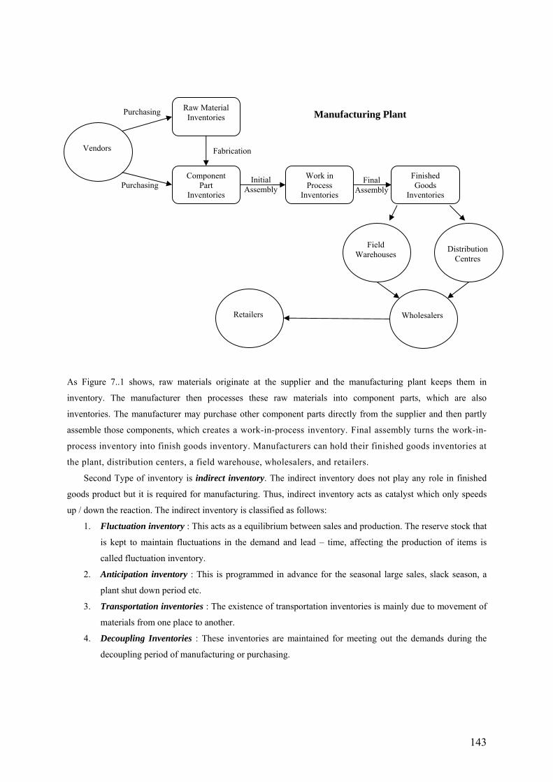
As Figure 7.1 shows, a materials flow system has inventories in various forms. Inventories for a manufacturing

facility consist of three major types, or accounting categories. Raw materials are the basic inputs to the

manufacturing process. Work in process consists of partially finished goods. Finished goods are the outputs of

the manufacturing process.

142

Raw Material Inventories

As Figure 7..1 shows, raw materials originate at the supplier and the manufacturing plant keeps them in

inventory. The manufacturer then processes these raw materials into component parts, which are also

inventories. The manufacturer may purchase other component parts directly from the supplier and then partly

assemble those components, which creates a work-in-process inventory. Final assembly turns the work-in-

process inventory into finish goods inventory. Manufacturers can hold their finished goods inventories at

the plant, distribution centers, a field warehouse, wholesalers, and retailers.

Second Type of inventory is indirect inventory. The indirect inventory does not play any role in finished

goods product but it is required for manufacturing. Thus, indirect inventory acts as catalyst which only speeds

up / down the reaction. The indirect inventory is classified as follows:

1. Fluctuation inventory : This acts as a equilibrium between sales and production. The reserve stock that

is kept to maintain fluctuations in the demand and lead – time, affecting the production of items is

called fluctuation inventory.

2. Anticipation inventory : This is programmed in advance for the seasonal large sales, slack season, a

plant shut down period etc.

3. Transportation inventories : The existence of transportation inventories is mainly due to movement of

materials from one place to another.

4. Decoupling Inventories : These inventories are maintained for meeting out the demands during the

decoupling period of manufacturing or purchasing.

Component Part

Inventories

Work in Process

Inventories

Finished Goods

Inventories

Field Warehouses

Distribution

Centres

Wholesalers

Retailers

Purchasing Manufacturing Plant

Vendors Fabrication

Initial Final Purchasing Assembly Assembly

143

7.3 How to Measure Inventory

Inventory is a hot topic in manufacturing circles today. Managers closely monitor and control

inventories to keep them as low as possible while still providing acceptable customer service.

To monitor and control inventories, managers need ways to measure inventories. Typically

inventories are measured in three ways: average aggregate inventory value, weeks of supply and

inventory turnover.

Measuring inventories begins with a physical count of units, or a physical measurement of

volume or weight. Because the monetary value of various units may vary a great deal, managers use the

average aggregate inventory value to calculate the average total value of all items held in inventory

during some time period. We compute the average aggregate inventory value by multiplying the average

number of units of each item (the beginning inventory plus ending inventory, divided by two) by its per

unit value to obtain the total average value of each item and then add the total average values of all

items. The average aggregate inventory value tells the inventory manager just how much of the

company's total assets are invested in inventory.

To calculate the second measure of inventory, weeks of supply, divide the average aggregate

inventory value by the value of the sales per week. The numerator of this measure includes the value of

all inventory items (raw materials, work in process, and finished goods), whereas the denominator

includes only the cost of the finished goods sold.

To calculate the third measure of inventory, inventory turnover (turns), divide the annual value

of the sales by the average aggregate inventory value maintained during the year.

7.4 Reasons for Holding Inventories

Inventories serve a number of important functions in various companies. Among the major reasons for

holding inventories are

1. To satisfy expected demand. Companies use anticipation stock ( buffer stock) to satisfy expected

demand, and it is particularly important for products that exhibit marked seasonal demand but are

produced at uniform rates. Air conditioner, rain suit manufacturers and children's toy manufacturers

build up anticipation stock, which is depleted during peak demand periods.

2. To protect against stock outs. Manufacturers use safety stock to protect against uncertainties in

either the demand or supply of an item. Delayed deliveries and unexpected increases in demand

increase the risk of shortages. Safety stock provides insurance that the company can meet

anticipated customer demand without backlogging orders. In Figure 7.1, the plant can invest in

safety stocks at several points. Raw materials and component parts can have safety stocks within the

manufacturing plant. Finished goods can have safety stocks throughout the materials flow (at the

plant, field warehouses, distribution centers, wholesalers, and retailers).

3. To take advantage of economic order cycles. Companies use cycle stock to produce (or buy) in

quantities larger than their immediate needs. Because of the cost involved in setting up a machine,

companies usually find producing in large quantities economical. Similarly, to minimize purchasing

costs companies often buy in quantities that exceed their immediate requirements. In both cases,

periodic orders, or order cycles, produce more economical overall production costs. The quantity

144

produced is called the economic lot size. The quantity ordered is called the economic order quantity

(EOQ).

4. To maintain independence of operations. The successive stages in the production and distribution

system require a buffer of inventories between them so that they can maintain their independence of

operations, for example, the raw materials inventory buffers the manufacturer from problems with a

supplier. Similarly, the finished goods inventory buffers factory operations from problems in the

distribution system.

5. To allow for smooth and flexible production operations. A production-distribution system needs

flexibility and a smooth flow of material, but production cannot be instantaneous so work-in-process

inventory relieve pressure on the production system. Similarly, manufacturers use in-transit or

pipeline inventory to offset distribution delays. Both work-in-process inventories and pipeline

inventories are part of a broader classification, called movement inventories.

6. To guard against price increases. Manufactures sometimes use large purchase, or large production

runs, to achieve savings when they expect price increases for raw materials or component parts.

7.5 Objectives of inventory control

Inventory control has two major objectives. The first objective is to maximize the level of

customer service by avoiding under stocking. Under stocking causes missed deliveries, backlogged

orders, lost sales, production bottlenecks, and unhappy customers.

The second objective of inventory control is to promote efficiency in production or purchasing

by minimizing the cost of providing adequate level of customer service. Placing too much emphasis on

customer service can lead to over stocking, which means the company has tied up too much of its capital

in inventories.

These two objectives often conflict. Achieving high levels of customer service by maintaining certain

inventories leads to higher inventory costs and less efficiency in production or purchasing. Inventory control

becomes a balancing act. Many a times a manager selects a desired level of customer service and attempts to

control inventory in a manner that achieves that level of customer service at the lowest cost possible. Thus the

problem is striking a balance in inventory levels, avoiding both overstocking and understocking.

The basic purpose of inventory analysis in manufacturing and stock keeping services is to specify

(1) when items should be ordered (when to order)and

(2) how large the order should be (how much to order).

Many firms are tending to enter into longer-term relationships with vendors to supply their needs for perhaps the

entire year. This changes the "when" and "how many to order" to "when" and "how many to deliver."

In this chapter, we will try to answer these questions under variety of circumstances.

In making decisions about inventory levels, companies must address a variety of costs. Hence,

before we proceed to answer the above two questions, let us discuss about the costs involved in inventory

decisions.

145

7.6 Costs Involved In Inventory Problems :

The costs play an important role in making a decision to maintain the inventory in the organization.

These costs are as follow :

1. Purchase Cost :

The actual price paid for the procurement of items is called purchase cost. The purchase cost becomes

relevant if a quantity discount is available. A company offering quantity discounts drops the price per

item when the order is sufficiently large. This becomes an incentive to order greater quantities.

For us, in this chapter we will assume that it is independent of the size of the quantity ordered (or

manufactured) or in other words, quantity discounts are not available.

2. Inventory Holding Cost :

The holding, carrying or storage cost is the cost associated with maintaining an inventory until

it is used or sold. Holding or storage cost includes the cost of maintaining storage facilities, the

cost of insuring the inventory, taxes attributed to storage, costs associated with obsolescence,

and costs associated with the capital that is committed to the inventory. The latter is called the

opportunity cost, an expense incurred by having capital tied up in inventory rather than having it

invested elsewhere, and it is frequently the most important component of the inventory holding

cost. The opportunity cost is generally equal to the biggest return that the company could obtain

from alternative investments. The holding or storage cost is usually related to the maximum

quantity, average quantity, or excess of supply in relation to demand during a particular time

period. For example, a company could estimate that its annual inventory holding cost is

approximately 13 to 15 percent of the original purchase price of the commodity. So another

common practice is to estimate the annual holding costs as a percentage of the unit cost of the

item.

3. Shortage Cost :

The stock out or shortage cost occurs when the demand for an item exceeds its supply. When a stock

out or shortage occurs, a company faces two possibilities:

• It can meet the shortage with some type of rush, special handling or priority shipment.

• It cannot meet the shortage at all.

The cost associated with a stock out or shortage depends on how the company handles the problem.

Consider first the cost incurred when the inventory is on back order. In theory, demand for the back-

ordered item is satisfied when the item next becomes available. From a practical standpoint, accurately

determining the nature and magnitude of the back-ordering cost can be difficult. A small portion of the

back-ordering cost, such an the cost of notifying the customer that the item has been back ordered and

when delivery can be expected, may be fairly easy to determine. Another portion of the back-ordering

cost may involve explicit costs for overtime, special clerical and administrative costs for expediting, and

extraordinary transportation charges. Such costs are much more difficult to determine. Finally, a major

portion of the back-ordering cost is an implicit cost - it reflects the loss of the customer's goodwill. This

is a difficult cost to measure, because it is a penalty cost that accounts for lost future sales, for example,

an equipment retailer might have a shortage cost composed primarily of loss goodwill, which it can

146

estimate as 15 percent of the original purchase cost of the equipment. But when back ordering is not

possible or the customer chooses to order from another company, the shortage costs include the costs of

notifying the customer, the loss in profit, from the sale, and the future loss of goodwill.

The shortage cost may also depend on the size of the shortage and how long the shortage lasts. For

example, customers may have written into their purchase contracts specific penalty clauses that are

based on shortage amounts and times. In other instances the shortage cost may be a fixed amount

regardless of the number of units unavailable or how long the shortage exists.

4. Set-Up Cost ( or the ordering cost):

Each time a company places a purchase order with a supplier or a production order with its own shop, it

incurs an ordering cost. To buy an item someone has to solicit and evaluate bids, negotiate price terms,

decide how much to order, prepare purchase orders, and follow up to make sure that the shipment arrives

on time. For example, when we order an item from a supplier, we might incur a Rs.100 cost for placing

the order and a cost of Rs.5 for each unit we are ordering. The purchasing cost function for this situation

is Rs.100 + Rs.5x where x is the number of units. The fixed portion (Rs.100) of the total purchasing

cost is independent of the amount ordered; it is primarily the cost of the clerical and administrative

work. Placing a production order for a manufacturing item involves many of the same activities; only the

type of paperwork changes.

The setup cost is the cost involved in changing a machine over to produce a different part or item. While

someone is adjusting a machine, it is idle and the company incurs the additional costs of the setup

workers. Sometimes the machines are producing trial products, and they will make defective parts until

the machine is fine-tuned. For example, we have a production process for manufacturing TV cabinets.

The setup cost for a production run is Rs.1,000, and each TV cabinet costs Rs. 55 to manufacture. The

manufacturing cost function for this situation is Rs.1,000 + 55x where x is the number of TV cabinets.

Companies treat setup costs as a fixed cost and try to make the production lot size as big as possible to

spread the setup cost over as many units as possible.

5. Total Inventory Cost :

If price discounts are available, then we should formulate total inventory cost by taking sum of

purchase cost (PC), Inventory Holding Cost (IHC), Shortage Cost (SC) and Ordering Cost (OC). Thus, the total

inventory cost; TC, is given by

TC = PC + IHC + SC + OC

When price discounts are not offered then total cost (TC) is given by

TC = IHC + SC + OC

Establishing the correct quantity to order from vendors or the size of lots submitted to the firm's productive

facilities involves a search for the minimum total cost resulting from the combined effects of four individual costs:

holding costs, setup costs, ordering costs, and shortage costs. Of course, the timing of these orders is a critical

factor that may impact inventory cost.

147

Apart from costs, the other variables which play an important role in decision making are as follows:

1. Demand :

The size of the demand is the number of units required in each period. It is not necessarily the amount

sold because demand may remain unfulfilled due to shortage or delays. The demand pattern of the items may be

either deterministic or probabilistic. In the deterministic case, the demand over a period is known. This known

demand may be fined or variable with time. Such demand is known as static and dynamic respectively. When

the demand over as period is uncertain but can be predicted by a probability distribution, we say it is a case of

the probabilistic demand. A probabilistic demand may be stationary or non-stationary over time.

Independent versus Dependent Demand

In inventory management, it is important to understand the difference between dependent and

independent demand. The reason is that entire inventory systems are predicated on whether demand is derived

from an end item or is related to the item itself.

Briefly, the distinction between independent and dependent demand is this: In independent demand, the

demands for various items are unrelated to each other. For example, a workstation may produce many parts that are

unrelated but meet some external demand requirement. In dependent demand, the need for any one item is a direct

result of the need for some other item, usually a higher-level item of which it is part.

In concept, dependent demand is a relatively straightforward computational problem. Needed quantities

of a dependent-demand item are simply computed, based on the number needed in each higher-level item in which

it is used. For example, if an automobile company plans on producing 500 cars per day, then obviously it will need

2.000 wheels and tires (plus spares). The number of wheels and tires needed is dependent on the production levels

and is not derived separately. The demand for cars, on the other hand, is independent—it comes from many sources

external to the automobile firm and is not a part of other products; it is unrelated to the demand for other products.

To determine the quantities of independent items that must be produced, firms usually turn to their sales

and market research departments. They use a variety of techniques, including customer surveys, forecasting

techniques, and economic and sociological trends as we discussed in the previous Chapter 6 on forecasting

techniques. Because independent demand is uncertain, extra units must be carried in inventory. This chapter

presents models to determine how many units need to be ordered, and how many extra units should be carried to

reduce the risk of stocking out.

2. Lead – Time :

It is the time between placing an order and its realization in stock. It can be deterministic or

probabilistic. If both demand and lead–time are deterministic, one needs to order in advance by a time equal to

lead-time. However, if lead-time is probabilistic, it is very difficult to answer - when to order?

3. Cycle Time :

The cycle time is time between placements of two orders. It is denoted by T. It can be determined in

one of the two ways.

I) Continuous Review : Here the number of units of an item on hand is known. In this case,

an order of fixed size is placed every time the inventory level reaches at a pre-specified

148

level, called reorder level. Many authors referred this as the two-bin systems or fixed

order level system.

II) Periodic Review : Here the orders are placed at equal interval of time and size of the order

depends on the inventory on hand and on order at the time of the review. This is also

called the fixed order interval system

4. Planning Horizon :

The period over which a particular inventory level will be maintained is called planning horizon. It

may be finite or infinite. It is denoted by H.

7.7 Deterministic Continuous Review Models :

Notations :

We shall use the following notations for the discussion of models in the chapter.

C : Purchase or manufacturing cost of an item.

Co: The ordering cost per order.

Ch : Inventory holding cost of an item per unit per time unit.

Cs : Shortage cost per unit short per time.

D : Demand rate of an item.

Q : Order quantity (a decision variable).

T : Cycle time (a decision variable).

ROL : Reorder level i.e. the level of inventory at which an order is placed.

L : Lead – Time.

N : Number of orders per time unit.

T : Production time period.

P : Production rate at which quantity is produced.

PC : Total purchase cost.

IHC : Total inventory holding cost per time unit

SC : Total shortage cost per time unit

OC : Ordering cost per order.

TC : Total inventory cost per time unit.

TVC : Total variable inventory cost per time unit.

The parameters are defined with proper units.

7.7.1 Economic Order Quantity (EOQ) Model With Constant Rate Of Demand :

EOQ is one of the oldest and most commonly known techniques. This model was first developed by

Ford Harris and R.Wilson independently in 1915. The objective is to determine economic order quantity, Q

which minimizes the total cost of an inventory system when demand occurs at a constant rate. The model is

developed under following assumptions:

149

The system deals with single item.

The demand rate of D units per time unit is known and constant.

Quantity discounts are not available.

The item is produced in lots or purchasers are made in orders. The ordering cost is constant.

Shortages are not allowed. Lead – Time is known and is constant.

Replenishment rate is infinite.

Replenishment size, Q, is the decision variable.

T is cycle time.

The inventory holding cost, Ch per unit per time unit is known and constant during the period under

review.

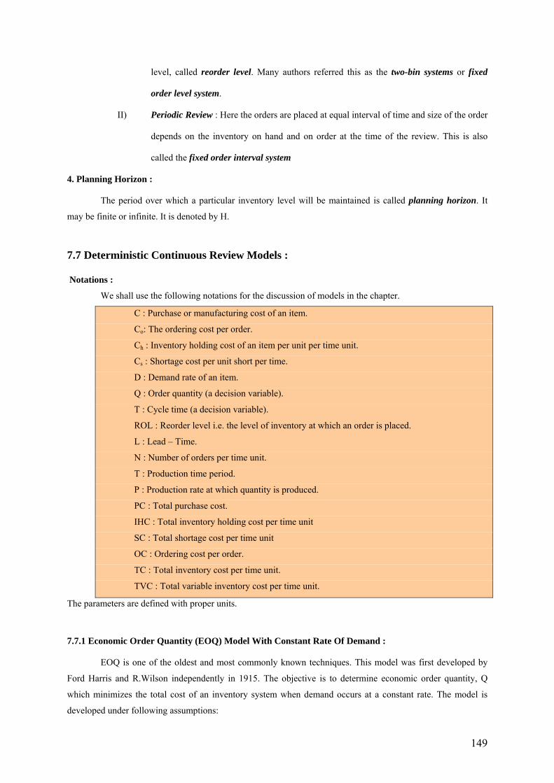
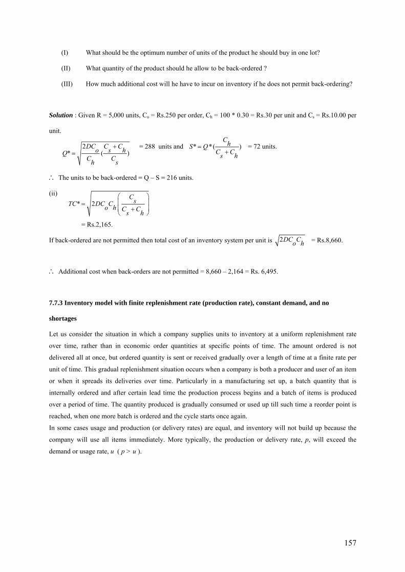
The following figure shows the graphic depiction of this particular inventory situation. Each inventory

cycle begins with the receipt of an order of Q units. i.e Q units are ordered and stocked in the system. Demand is

occurring at the rate of D units per time unit during cycle time T.

At the reorder point R, when the on-hand inventory is barely sufficient to satisfy demand during the lead

time, LT, an order of Q units is placed. Since the demand rate and the lead time are constant, the order of Q

units is received exactly when the inventory level reaches zero. This means that there are no shortages.

Q

Demand Rate D

Average Cycle Inventory, Q/2

The inventory level varies from Q to zero, so the average inventory level during the inventory cycle is Q/2.

So, the inventory holding cost is obtained by multiplying this quantity with the cost of holding one unit per time

unit. Hence, IHC = ( Q/2) Ch . This cost is a linear function of Q.

Time Between Orders

(Order Cycle) = Q / D

0

Reorder Point, R

R

Receive Order

Place Order

Lead Time

Maximum Inventory

Time

150

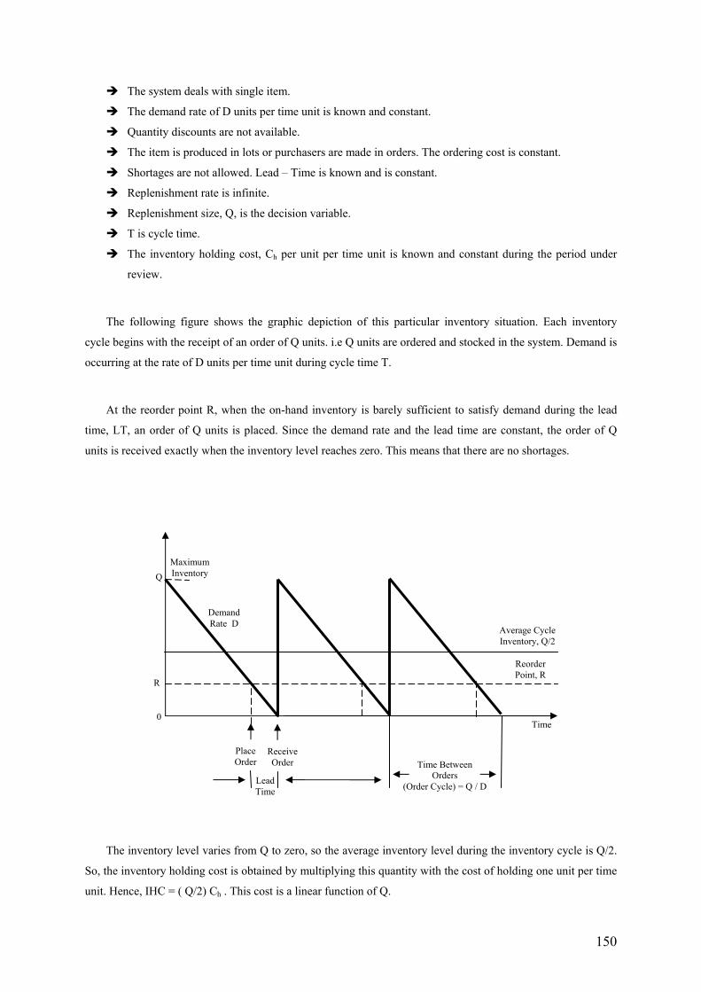
The number of orders placed during the planning horizon would be D/Q and hence the inventory ordering

cost OC will be a function of the number of orders placed and the ordering cost per order.

Thus, OC = ( D/Q) Co. Because the number of orders made in the planning horizon, D/Q, decreases as the

order size, Q, increases, OC is inversely proportional to Q.

The cost of the individual item is assumed to be constant, regardless of the size of the order. So the

purchase cost of the item is a horizontal line as shown in the following figure. It only increases the total

inventory cost by the constant amount, DC, during the entire quantity range. It does not affect the optimal order

quantity, Q*. Therefore, it is not really a relevant cost for the economic order quantity decision and we can

eliminate it from further consideration in the model.

Hence,

Total Inventory Cost TC = Ordering cost + holding cost

TC = ( D/Q) Co + ( Q/2) Ch

The total cost curve is U-shaped and reaches its minimum at the quantity for which the carrying and the

ordering costs are equal. We can equate both these values to obtain the optimal order quantity Q*.

Alternatively, we can use calculus to obtain the expression for Q*, setting the first derivative of TC to zero

and solving for Q.

Thus,

Also, since (d2TC/dQ2) > 0, Q* is minimum.

( ) ( )0 2

( ) 002 2

2* 0

D QTC C ChQCdTC D hC

dQ Q

DCQ

Ch

= +

−= + =

=

Purchase Cost

Total Cost

Annual Holding Cost Cost

Ordering Cost

Q* Order Quantity

151

The resulting expression of Q* obtained above is called the economic order quantity or the economic lot size.

The number of orders during the planning horizon is = D/Q*

The length of the order cycle t is = Q*/D

And the minimum total inventory cost TC* = ( D/Q*) Co + ( Q*/2) Ch = 2DC Co h

Note:

(1)Over a period of time, a company can use two policies for making inventory decisions. First, it can keep the

order size small. This will result in a small average inventory, and inventory carrying costs will be low. But this

policy will lead to frequent orders, and the total ordering costs will increase. Second, the company can increase

its order size. This will result in less frequent orders, so the total ordering costs will be low. But this will result

in a high average inventory, and the total inventory carrying costs will increase.

(2) If unit cost is taken into account then TC = CD + ( D/Q) Co + ( Q/2) Ch

Sensitivity of lot-size model :

For the lot-size model, we have total cost of an inventory system per time unit as TC = ( D/Q*) Co + ( Q*/2) Ch

and Q* as given above. Now suppose that instead of ordering for Q0 – units (given as Q* above) and suppose

that for it the total cost of the inventory system is TC(Q0 ), we replenish another lot-size (say) Q1. Such that Q1 =

bQ0,

b > 0 and let TC1 (Q1) be the corresponding total cost of an inventory system.

The ratio is known as the measure of sensitivity of the lot-size model. 1 1 2( ) 1( ) 20

TC Q bTC Q b

+=

Limitations Of The EOQ Formula :

Note that the EOQ formula is derived under several rigid assumptions which give rise to limitation on its

applicability.

In practice, the demand is neither known with certainty nor is uniform over the time period. If the

fluctuations are mild, the formula is practically valid; but when fluctuations are wild, the formula

looses its validity.

It is not easy to measure the inventory holding cost and the ordering cost accurately. The ordering cost

may not be fixed but will depend on the order quantity Q.

The assumptions of zero lead-time and that the inventory level will reach to zero at the time of the next

replenishment is not possible.

The stock depletion is rarely uniform and gradual.

One may have to take into account the constraints of floor-space, capital investment, etc in stocking the

items in the inventory system.

Example 7.1 : Using the following information, obtain the EOQ and the total variable cost associated with the

policy of ordering quantities of that size. Annual demand = 20,000 units, ordering cost = Rs. 150 per order, and

inventory carrying cost is 24% of average inventory value.

152

Solution : Given D = 20,000 units, Co = Rs. 150 / order, Ch = Rs. 0.24 / unit / annum. Then using the above

formulas for Q and TC,

Q* = 5000 units and TC (Q*) = Rs. 1,200.

Example 7.2 : An oil engine manufacturer purchases lubricants at the rate of Rs. 42 per piece from a vendor.

The requirement of these lubricants is 1,800 per year. What should be the order quantity per order, if the cost per

placement of an order is Rs.16 and inventory carrying charge per rupee per year is 20 paise.

Solution : Given D = 1,800*42 = 75,600 units, Co = Rs.16 / order and Ch = 0.20 per unit / year. Then

Q* = 34,776 units.

Thus, the optimum inventory quantity of lubricant at the rate of Rs.42 per lubricant =Q*/42 = 83 lubricants.

Example 7.3 : A company uses rivets at a rate of 5,000 kg per year, rivets costing Rs.2 per kg. It costs Rs.20 to

place an order and the carrying cost of inventory is 10 % per annum. How frequently should order for rivets be

placed and how much?

Solution : Given D = 5,000 kg / year. C = Rs.2 / kg., Co = Rs. 20 / order and Ch = 2 * 10 % per unit/year.

Then Q* = 1,000 kgs. and T* = Q*/D = 1/5 years = 2.4 months.

Example 7.4 : A supplier ships 100 units of a product every Monday. The purchase cost of product is Rs.60 per

unit. The cost of ordering and transportation from the supplier is Rs.150 per order. The cost of carrying

inventory is estimated at 15 % per year of the purchase cost. Find the lot-size that will minimize the cost of the

system. Also determine the optimum cost.

Solution : Given D = 100 units per week, Co = Rs.150 /order, Ch = 15% of 60 = Rs. 9 per unit / year = Rs.9/52

per unit / week. Then Q*= 416 units, and optimum cost = CD + TC(Q*) = Rs.6,072

7.7.2 EOQ Model with constant demand and shortages allowed:

The inventory problem in the above section becomes slightly more complicated when a company permits

shortages, or backorders, to occur. However, in many situations shortages are economically desirable.

Permitting shortages allows the manufacturer or retailer to increase the cycle time, thereby spreading the setup

or ordering cost over a longer time period. Allowing shortages may also be desirable when the unit value of the

inventory and therefore the inventory holding cost is high.

In the back order situation customers place an order, no stock is available, and they simply wait until stock

becomes available, at which point the order is filled. The company hopes that the waiting period for the back

order will be short and its customers will be patient.

For this model we will use the assumptions of a known and constant demand rate and instantaneous delivery of

goods to inventory like the basic EOQ model. If S represents the amount of the shortage ( size of the back order)

that has accumulated when the new shipment of size Q arrives, the economic order quantity model with constant

demand and permissible shortages has the following major characteristics and graphic depiction.

153

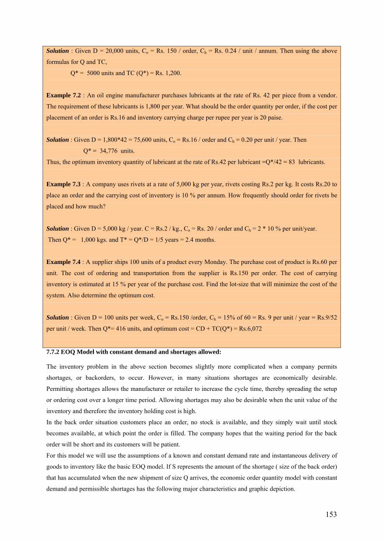
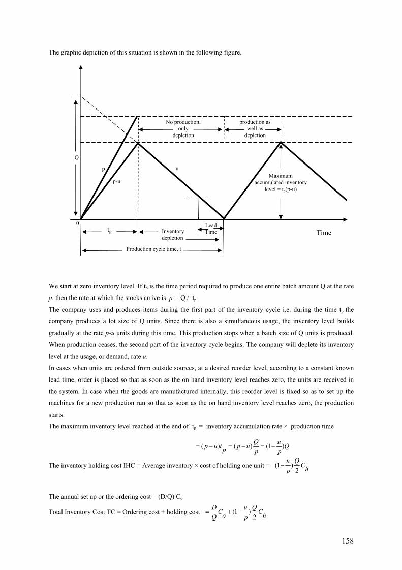
Maximum inventory Q-S

When the new shipment of size Q arrives, the company immediately ships the back orders of size S to

the customers. The remaining units Q-S immediately go into inventory.

The inventory level will vary from a minimum of -S units to a maximum of Q-S units.

The inventory cycle of T units is divided into two distinct parts: t1 when inventory is available for

filling orders and t2 when inventory is not available, stock outs occur, and back orders are made.

Here apart from the notations introduced in the previous model we introduce two new notations as follows:

Cs : cost of back order, per unit per unit time

S : the number of units short or back ordered.

Now,

The inventory ordering cost is a function of the number of orders made, D/Q, and the inventory ordering cost

per order, Co.

OC =No. of orders × Cost per order = (D/Q)Co

Also we know that t1 = (Q-S)/D and t2 = S/D

The inventory holding cost can be calculated from the figure as:

The average inventory for the time period t = [ (Avg. inventory over t1) + (Avg. inventory over t2) ] / t

The positive inventory level ranges from Q-S to 0. This means that the average inventory level is (Q-S)/2 for the

time period t1. For t2 it is 0.

IHC = Average inventory × cost of holding one unit

0

Q-S

Q

Time S

-S

t1 t2

t

0 2( )1 222

Q S t t Q SC Ch ht Q

−⎛ ⎞+⎜ ⎟ −= ==⎜ ⎟⎜ ⎟⎜ ⎟⎝ ⎠

154

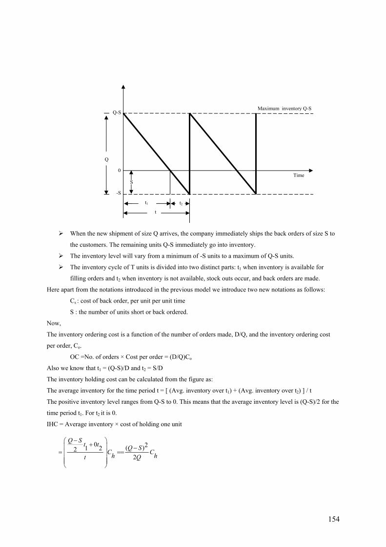
The backordering cost is computed in a similar way. From the figure we can see that the shortage ranges from 0

units to S units. This means that the average shortage is S/2 while there are shortages i.e during the time period

t2.

SC = Average number of units short × cost of one unit being short

For this inventory model the total cost is calculated as

2222

S t SC Cs s= =t Q

TC = ordering cost + holding cost + shortage cost = OC + IHC + SC

2 2( )2 2

D Q S SC Co hQ Q Q−

Cs+= +

Since TC is a function of two variables Q and S, therefore to determine the optimal order size and the optimal

shortage level S, we need to differentiate the total variable cost function with respect to Q and S, set the two

resulting equations equal to zero and solve them simultaneously. By doing so, we get the following results

2* (

* *( )

DC C Co s hQC Ch s

ChS QC Cs h

+=

=+

)

The number of orders for the planning horizon = D/Q*

The maximum inventory level = Q* - S*

The average positive inventory level is = (Q* - S*) / Q*

The length of time during which there are no shortages = t1* = (Q* - S*) / D

The length of time during which there are shortages = t2* = S* / D

The length of the inventory cycle = t* = Q* / D

The minimum total inventory cost during the planning horizon = TC* 2 2( * *) *

* 2 * 2 *D Q S SC Co hQ Q Q

− Cs+= +

* 2CsDC Co h C Cs h

⎛ ⎞⎜ ⎟=⎜ ⎟+⎝ ⎠

TCWhen values of Q* and S* are substituted, we get

Example 7.5 : The demand for a certain item is 16 units per period. Unsatisfied demand causes a shortage cost

of Rs.0.75 per unit per short period. The cost of initiating purchasing action is Rs. 15.00 per purchase and the

holding cost is 15% of average inventory valuation per period. Item cost is Rs. 8.00 per unit. Find the minimum

cost and purchase quantity.

Solution : Given D = 16 units, Cs = Rs.0.75 per unit short, Ch = Rs. 8 * 15% = Rs. 1.20 and Co = Rs.15.00 /

order.

155

Using the formulas for Q* and TC* as

We get Q* = 32 units (approx.) and TC* = Rs.14.88 (approx.)

2* ( )

DC C Co s hC Ch s

+= * 2

CsTC DC Co h C Cs h

⎛ ⎞⎜ ⎟=⎜ ⎟+

Q

⎝ ⎠

Example 7.6 : A television manufacturing company produces its own speakers, which are used in the

production of its television sets. The television sets are assembled on a continuous production line at rate of

8,000 per month. The company is interested in determining when and how much to procure, given the following

information:

(I) Each time a batch is produced, a set-up cost of Rs.12,000 is incurred.

(II) The cost of keeping a speaker in stock is Rs. 0.30 per month.

(III) The production cost of a single speaker is Rs.10.00 and can be assumed to be a unit cost.

(IV) Shortage of a speaker, (if there exists) costs Rs. 1.10 per month.

Solution : Given D = 8,000 televisions per month, Co = Rs.12,000 per production run, Ch = Rs.0.30 per unit per

month, Cs = Rs.1.10 per unit short per month.

Case (i) When Shortages are not allowed, = 25,298 speakers and T = Q*/D = 3.2 months. 2Q =*

DCoCh

Thus, 25,298 speakers are to be produced every 3.2 months.

Case (ii) When shortages are permitted = 28,540 speakers and T = Q*/D = 3.6

months

2Q* ( )

DC C Co s hC Ch s

+=

Hence, when shortages are permitted, 28,540 speakers are produced at every 3.6 months.

Optimal number of speakers stored = = 22,424 speakers. *( )C

Q sC Cs h+

Thus, a shortage of 6,116 (= 28,540 – 22,424) speakers is permitted.

Or else optimal shortage level = = 6116 ( approx.) * *( )C

S Q hC Cs h

=+

Example 7.7 : A dealer supplies you the following information with regard to a product dealt in by him :

Annual demand = 5,000 units, ordering cost = Rs.25.00 per order, inventory carrying cost is 30% per unit per

year of purchase cost Rs.100 per unit.

The dealer is considering the possibility of allowing some back-orders to occur for the product. He has

estimated that the annual cost of back-ordering the product will be Rs.10.00 per unit.

156

(I) What should be the optimum number of units of the product he should buy in one lot?

(II) What quantity of the product should he allow to be back-ordered ?

(III) How much additional cost will he have to incur on inventory if he does not permit back-ordering?

Solution : Given R = 5,000 units, Co = Rs.250 per order, Ch = 100 * 0.30 = Rs.30 per unit and Cs = Rs.10.00 per

unit.

= 288 units and = 72 units.

∴ The units to be back-ordered = Q – S = 216 units.

(ii)

= Rs.2,165.

If back-ordered are not permitted then total cost of an inventory system per unit is = Rs.8,660.

∴ Additional cost when back-orders are not permitted = 8,660 – 2,164 = Rs. 6,495.

7.7.3 Inventory model with finite replenishment rate (production rate), constant demand, and no

shortages

Let us consider the situation in which a company supplies units to inventory at a uniform replenishment rate

over time, rather than in economic order quantities at specific points of time. The amount ordered is not

delivered all at once, but ordered quantity is sent or received gradually over a length of time at a finite rate per

unit of time. This gradual replenishment situation occurs when a company is both a producer and user of an item

or when it spreads its deliveries over time. Particularly in a manufacturing set up, a batch quantity that is

internally ordered and after certain lead time the production process begins and a batch of items is produced

over a period of time. The quantity produced is gradually consumed or used up till such time a reorder point is

reached, when one more batch is ordered and the cycle starts once again.

In some cases usage and production (or delivery rates) are equal, and inventory will not build up because the

company will use all items immediately. More typically, the production or delivery rate, p, will exceed the

demand or usage rate, u ( p > u ).

2* ( )

DC C Co s hQC Ch s

+=

* *( )S QCh

C Cs h=

+

* 2CsTC DC Co h C Cs h

⎛ ⎞⎜ ⎟=⎜ ⎟+⎝ ⎠

2DC Co h

157

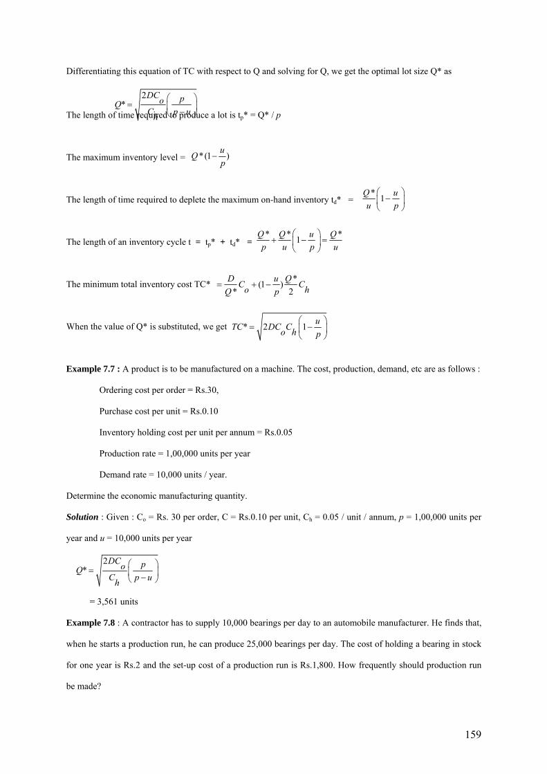
The graphic depiction of this situation is shown in the following figure.

We start at zero inventory level. If tp is the time period required to produce one entire batch amount Q at the rate

p, then the rate at which the stocks arrive is p = Q / tp.

The company uses and produces items during the first part of the inventory cycle i.e. during the time tp the

company produces a lot size of Q units. Since there is also a simultaneous usage, the inventory level builds

gradually at the rate p-u units during this time. This production stops when a batch size of Q units is produced.

When production ceases, the second part of the inventory cycle begins. The company will deplete its inventory

level at the usage, or demand, rate u.

In cases when units are ordered from outside sources, at a desired reorder level, according to a constant known

lead time, order is placed so that as soon as the on hand inventory level reaches zero, the units are received in

the system. In case when the goods are manufactured internally, this reorder level is fixed so as to set up the

machines for a new production run so that as soon as the on hand inventory level reaches zero, the production

starts.

The maximum inventory level reached at the end of tp = inventory accumulation rate × production time

The inventory holding cost IHC = Average inventory × cost of holding one unit =

The annual set up or the ordering cost = (D/Q) Co

Total Inventory Cost TC = Ordering cost + holding cost

0 Lead Time tp Inventory

depletion

No production; only

production as well as

depletion depletion

Q

Maximum accumulated inventory

level = tp(p-u)

u p

p-u

Time

Production cycle time, t

( ) ( ) (1 )Q up u t p u Qp p p= − = − = −

(1 )2

u Q Chp−

(1 )2

D u QC Co hQ p= + −

158

Differentiating this equation of TC with respect to Q and solving for Q, we get the optimal lot size Q* as

The length of time required to produce a lot is tp* = Q* / p

2*

DC po

The maximum inventory level =

The length of time required to deplete the maximum on-hand inventory td* =

The length of an inventory cycle t = tp* + td* =

The minimum total inventory cost TC*

When the value of Q* is substituted, we get

Example 7.7 : A product is to be manufactured on a machine. The cost, production, demand, etc are as follows :

Ordering cost per order = Rs.30,

Purchase cost per unit = Rs.0.10

Inventory holding cost per unit per annum = Rs.0.05

Production rate = 1,00,000 units per year

Demand rate = 10,000 units / year.

Determine the economic manufacturing quantity.

Solution : Given : Co = Rs. 30 per order, C = Rs.0.10 per unit, Ch = 0.05 / unit / annum, p = 1,00,000 units per

year and u = 10,000 units per year

= 3,561 units

Example 7.8 : A contractor has to supply 10,000 bearings per day to an automobile manufacturer. He finds that,

when he starts a production run, he can produce 25,000 bearings per day. The cost of holding a bearing in stock

for one year is Rs.2 and the set-up cost of a production run is Rs.1,800. How frequently should production run

be made?

Q =C p uh

⎛ ⎞⎜ ⎟−⎝ ⎠

*(1 )uQp

−

* 1Q uu p

⎛ ⎞−⎜ ⎟

⎝ ⎠

* * 1Q Q u Q *p u p

⎛ ⎞+ − =⎜ ⎟

⎝ ⎠ u

*(1 )* 2

D u QC Co hQ p= + −

* 2 1 uDC Co h p⎛ ⎞

= −⎜ ⎟⎝ ⎠

TC

2*

DC poQC p uh

⎛ ⎞= ⎜ ⎟−⎝ ⎠

159

Solution : Given : Ch = Rs.2.00 / bearing / year = Rs.0.0055 / bearing / year, Co = Rs.1800 / production run,

u = 10,000 bearings/day, p = 25,000 bearings / day. Then using the above formula for Q*, we get

Q* = 1,04,447 bearings.

T = Q*/ u = 10.5 days.

Length of production cycle = t1 = Q*/ p = 4 days.

Thus, the production cycle starts at an interval of 10.5 days and production continues for 4 days.

Example 7.9 : Find the most economic batch quantity of a product on a machine if the production rate of that

item on the machine is 200 pieces per day and the demand is uniform at the rate of 100 pieces per day. The

ordering cost is Rs. 200 per batch and the cost of holding one item in inventory is Rs.0.81 per day. How will the

batch quantity vary if the production rate is infinite?

Solution : Given : Co = Rs.200 / order, Ch = Rs.0.81 / unit / day, u = 100 units / day, p = 200 units / day. Using

the above formula for Q* we get, Q* = 317 units.

Cycle time, T = Q*/ u = 3.17 days.

Length of production cycle, t1 = Q*/ p = 1.58 days.

If the production rate is infinite, i.e. P →∞ then = 222 units. 2

*DCoQ =Ch

7.8 THE CONTINUOUS REVIEW MODEL: When to order

Here we consider a continuous review inventory system. Here the inventory level is being monitored on a

continuous basis so that a new order can be placed as soon as the inventory level drops to the reorder point.

Personals, in practice, make a physical count of inventory at periodic intervals to decide how much of each item

to order. Using the continuous review system to determine when to reorder, we review the remaining

quantity of an item each time a withdrawal is made from inventory. In practice, operations managers

make a physical count of inventory at periodic intervals (daily, weekly, or monthly) to decide how much

of each item to order. Many small retailers use this approach, simply checking the quantities on shelves

and in the storeroom on a periodic basis. Another very elementary type of continuous review system is the

traditional two-bin system, which sets aside two containers, or bins, to hold the total inventory of an item. Items

are withdrawn from the first bin until it is empty, at which point it is time to reorder the quantity that will again

fill the bin. The second bin contains enough stock to satisfy demand until the order comes in, plus an extra

amount to provide a cushion against a stock out.

In recent years, two-bin systems have been largely replaced by computerized inventory systems. Each addition

to inventory and each sale causing a withdrawal are recorded electronically, so that the current inventory level

always is in the computer. Therefore, a computer will trigger a new order as soon as the inventory level has

160

dropped to the reorder point. The continuous review system is also called a reorder point (ROP) system, or a

fixed order quantity system. It is also called a (R,Q) policy.It works this way:

“Place an order for Q units whenever a withdrawal brings the inventory to the reorder point R.”

The continuous review system has only two parameters, Q and R, and each new order is of size Q. For a

manufacturer managing its finished products inventory, the order will be for a production run if size Q. For a

wholesaler or retailer, the order will be a purchase order for Q units of the product.

Let us address the question of “when to order”. At the time of placing a new order, the stock in hand should be

sufficient to meet the demand until the new order arrives.

When both demand and the lead time are deterministic ( known with certainty), the reorder level is calculated

as:

Reorder level (ROL) = Demand during the replenishment lead time = d × LT

Example : Demand for an item is 5200 units a year and the EOQ has been calculated as 250 units. If the lead

time is 2 weeks, then the ordering policy will be ROL = (5200 / 52) × 2 = 200 units.

This means that as soon as the stock level falls to 200 units an order equal to EOQ = 250 units should be placed.

This rule of ordering is applicable only if the lead time is shorter than the stock cycle. Here, the stock cycle is T

= Q*/d = 250/100 = 2.5 weeks.

But if the lead time is 3 weeks, then the ROL = 100 × 3 = 300 units. Since EOQ = 250 units, therefore stock

level varies between zero and 250 units. Thus lead time demand of 300 units suggests that there should be one

outstanding order. In such cases, an order is placed when

Lead time demand = stock on hand + stock on order

300 = stock on hand + 250

or ROL = Lead time demand – stock on hand

In general, an ordering policy is stated as: “when lead time is between n × T and (n+1) × T, order an amount Q*

whenever stock on hand falls to d × LT – n × Q*, where n is number of stock cycle and lead time exceeds cycle

time T”. For example, lead time of 3 weeks is between 2 and 3 stock cycles, so n = 2, then

ROL = d × LT – n × Q*

= 100 × 3 – 2 × 250

= 50 units.

i.e each time the stock on hand declines to 50 units, an order of 250 units is placed.

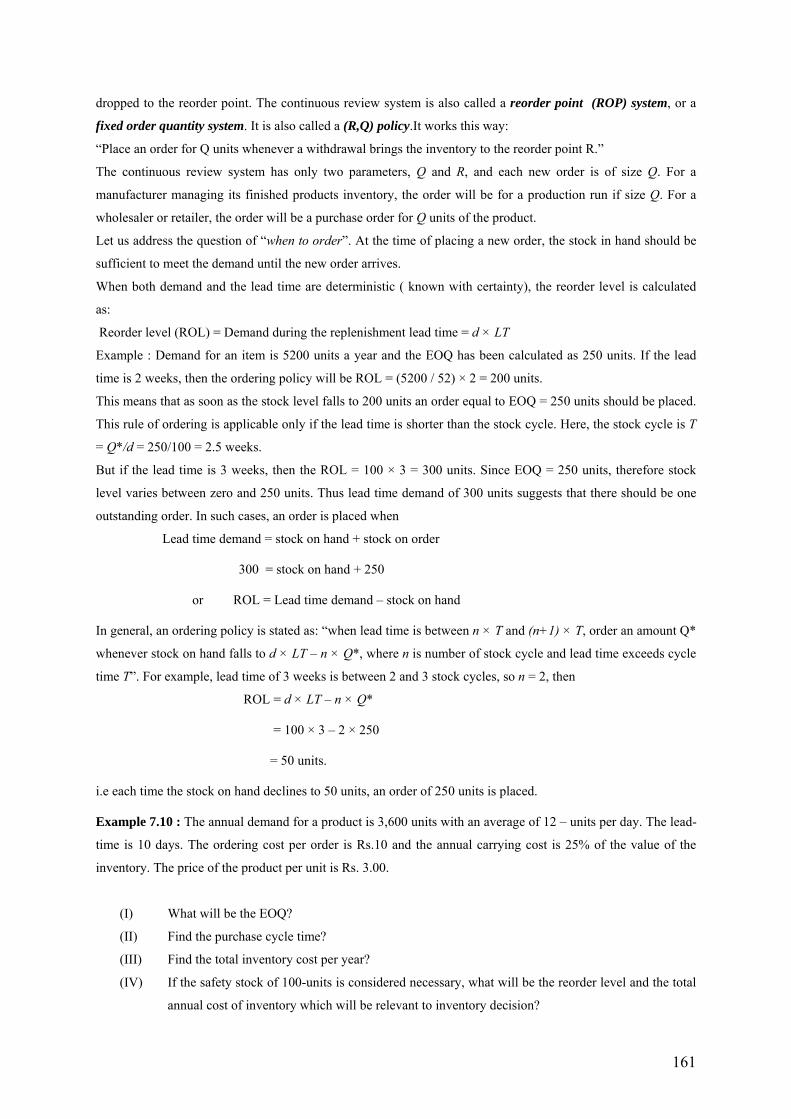
Example 7.10 : The annual demand for a product is 3,600 units with an average of 12 – units per day. The lead-

time is 10 days. The ordering cost per order is Rs.10 and the annual carrying cost is 25% of the value of the

inventory. The price of the product per unit is Rs. 3.00.

(I) What will be the EOQ?

(II) Find the purchase cycle time?

(III) Find the total inventory cost per year?

(IV) If the safety stock of 100-units is considered necessary, what will be the reorder level and the total

annual cost of inventory which will be relevant to inventory decision?

161

Solution : Given D = 3,600 units, Co = Rs. 20 per order, Ch = Rs. 3 * 25% per unit per year and lead-time = 10

days. Since, the demand is uniform at 12 – units per day, the total number of working days in the year = 3600/12

= 300.

The basic EOQ formula gives Q = 438 (appro.)

(ii) Cycle time = 438 / 12 = 36.5 days.

(iii) TC = CD + (D Co / Q) + ( Ch Q / 2) = Rs. 11128.60.

(iv) Re-order level = Safety stock + lead-time demand = 100 + 12 * 10 = 220 units.

∴ Average inventory = Safety stock + Q / 2 = 319 units.

∴ TC = (D Co / Q) + ( Ch Q / 2) = Rs. 164.38.

7.9 Operation Of Periodic Review System:

This system is also known as the fixed interval system or replenishment inventory system or cyclic review

system.

In this system, the size of order quantity may vary with the fluctuation in demand, but the ordering interval is

fixed. The system is specified for any item by

(1) review period t, and (2) replenishment level, or reoder level, R

In this system, the inventory position is periodically reviewed – once, weekly, monthly, quarterly or half-yearly.

At each review period, an order is placed for an amount equal to the difference between a fixed replenishment

level and the actual inventory level. The calculation of R is based on the formula:

Replenishment level R = Average consumption during a review period + Lead time + safety stock

Order quantity = Replenishment level – stock available

162

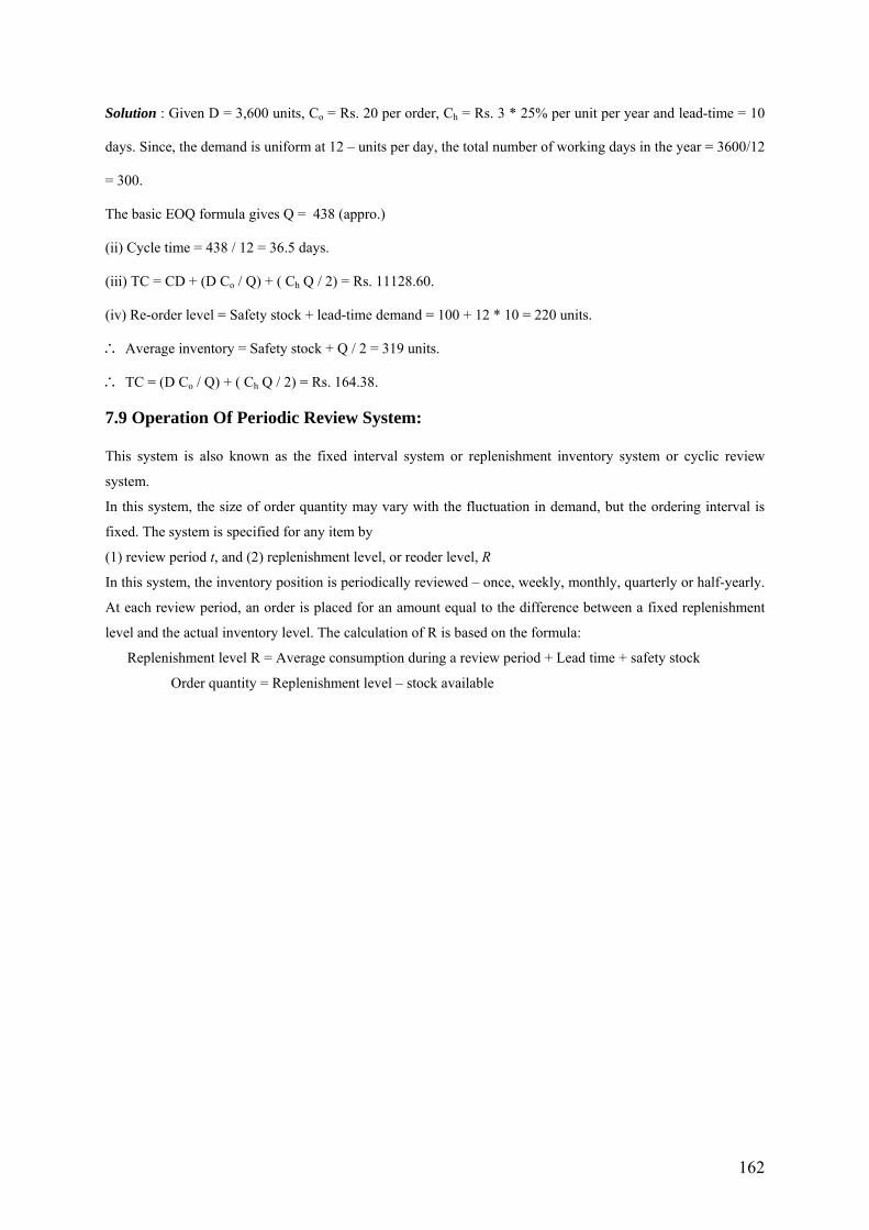
The following diagram gives the way in which the periodic review system operates.

Order Order quantity quantity

The order quantity is variable in size from one review date to another.

Example 7.11: For a periodic review system, find out the various parameters for an item with the following

data:

Annual consumption = 14000 units, Cost of one unit = Rs. 10, Supplier’s minimum quantity = 1000 units,

normal lead time = 10 days, maximum lead time = 15 days, maximum consumption = 1020 (average

consumption).

Solution: The maximum number of orders to cover the annual requirement is 140000 / 1000 = 14 orders.

Therefore, the review period should be 1/14th of an year or 26 days. We consider the period of review as 1

month instead of 26 days.

Now,

Safety stock = Max. consumption rate (review period + max. lead time) – normal consumption rate (review

period + normal lead time)

= 1.20 × (14000/12) ( 1 + (15/30)) – (14000/12) ( 1 + (10/30))

= 545 = approx. 550 units

Reorder level or replenishment level R = Average consumption rate × (review period + normal lead time) +

safety stock

= (14000/12) ( 1 + (10/30)) + 550 = 2105 units.

Maximum inventory when the supplies are received = 500 + order quantity

= 550 + (14000/12) = 1710 units

Maximum inventory = 550

Average inventory = (1710 + 550)/2 = 1130 units.

Time

Replenishment level

Review Max. demandpoint

Review pointInventory

level

Lead time

Safety stock

Review period

163

Probabilistic EOQ Model:

Stochastic or probabilistic inventory models are designed for analyzing inventory systems where there is a

considerable uncertainty about future demands. In such cases the demand is described by a probability

distribution. The models can further be categorized broadly under continuous and periodic review situations. In

this chapter we will consider only stochastic single period models without initial stock and without set up cost.

7.10 Stochastic Single – Period Models:

There are certain products which can be carried in inventory for only a very limited period of time before it can

no longer be sold. Such products are perishable products. For such products models called single period models

are designed. Following are such perishable products for which single period models are suitable:

Flowers, fresh foods, fruits, vegetables, fashion goods, seasonal goods, etc.

One important example of a perishable product is a daily news paper being sold at a news stand. A particular

day’s news paper can be carried in inventory for only a single day before it becomes outdated and needs to be

replaced by the next day’s news paper. When the demand for the news paper is a random variable, the owner of

the news stand needs to choose a daily order quantity that provides an appropriate trade-off between the

potential cost of over ordering (the wasted expense of ordering more than that can be sold) and the potential cost

of under ordering (the lost profit from ordering fewer than that can be sold). This problem is the classical

newsboy problem. Mathematically, it is termed as the single period stochastic or probabilistic model.

Model without set up cost:

Here we assume the following additional notations:

K = Set up cost per order

D = Probabilistic demand during the period

p(D) = probability density function of the demand during the period

Q = order quantity

x = the amount on hand before an order is placed

The assumptions are:

1. The model refers to a single perishable product involving a single time period because it cannot be sold

later

2. Demand is continuous and a random variable. The probability distribution of D is known

3. Demand occurs instantaneously at the start of the period immediately after the order is received.

4. No set up cost is incurred

5. There is no initial inventory on hand

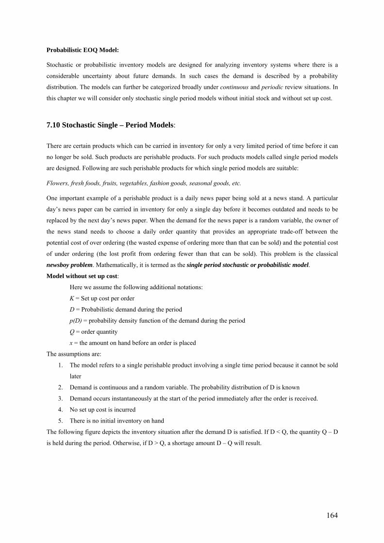
The following figure depicts the inventory situation after the demand D is satisfied. If D < Q, the quantity Q – D

is held during the period. Otherwise, if D > Q, a shortage amount D – Q will result.

164

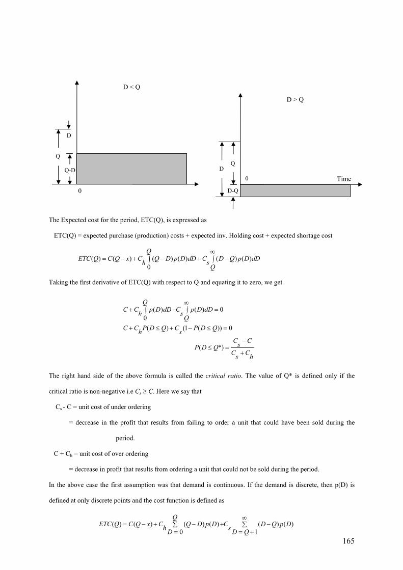
D < Q

D > Q

0

Q-D

D

Q Q

D

Time0

D-Q

The Expected cost for the period, ETC(Q), is expressed as

ETC(Q) = expected purchase (production) costs + expected inv. Holding cost + expected shortage cost

( ) ( ) ( ) ( ) ( ) ( )

0

QETC Q C Q x C Q D p D dD C D Q p D dDh s

Q

∞= − + − + −∫ ∫

Taking the first derivative of ETC(Q) with respect to Q and equating it to zero, we get

( ) ( ) 00( ) (1 ( )) 0

( *)

QC C p D dD C p D dDh s

QC C P D Q C P D Qh s

C CsP D QC Cs h

∞+ − =∫ ∫

+ ≤ + − ≤ =

−≤ =

+

The right hand side of the above formula is called the critical ratio. The value of Q* is defined only if the

critical ratio is non-negative i.e Cs ≥ C. Here we say that

Cs - C = unit cost of under ordering

= decrease in the profit that results from failing to order a unit that could have been sold during the

period.

C + Ch = unit cost of over ordering

= decrease in profit that results from ordering a unit that could not be sold during the period.

In the above case the first assumption was that demand is continuous. If the demand is discrete, then p(D) is

defined at only discrete points and the cost function is defined as

( ) ( ) ( ) ( ) ( ) ( )

0 1

QETC Q C Q x C Q D p D C D Q p Dh sD D Q

∞= − + − + −∑ ∑

= = + 165

The necessary optimality conditions are

( 1) ( ) ( 1) ( )ETC Q ETC Q and ETC Q ETC Q− ≥ + ≥

which further boils down to

( * 1) (

C CsP D Q P D QC Cs h

*)−

≤ − ≤ ≤ ≤+

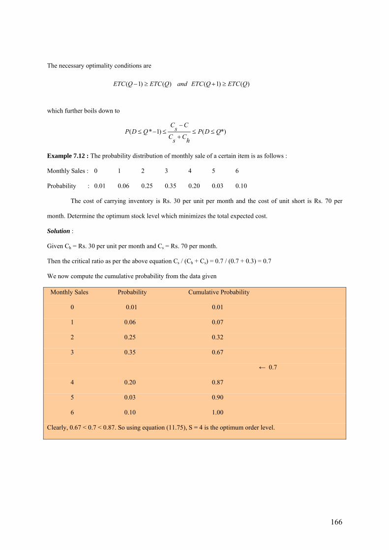
Example 7.12 : The probability distribution of monthly sale of a certain item is as follows :

Monthly Sales : 0 1 2 3 4 5 6

Probability : 0.01 0.06 0.25 0.35 0.20 0.03 0.10

The cost of carrying inventory is Rs. 30 per unit per month and the cost of unit short is Rs. 70 per

month. Determine the optimum stock level which minimizes the total expected cost.

Solution :

Given Ch = Rs. 30 per unit per month and Cs = Rs. 70 per month.

Then the critical ratio as per the above equation Cs / (Ch + Cs) = 0.7 / (0.7 + 0.3) = 0.7

We now compute the cumulative probability from the data given

Monthly Sales Probability Cumulative Probability

0 0.01 0.01

1 0.06 0.07

2 0.25 0.32

3 0.35 0.67

← 0.7

4 0.20 0.87

5 0.03 0.90

6 0.10 1.00

Clearly, 0.67 < 0.7 < 0.87. So using equation (11.75), S = 4 is the optimum order level.

166

REVIEW EXERCISE

Q. An aircraft company uses rivets at an approximate demand rate of 2,500 kg per year. Each unit costs Rs. 30

per kg and the company personnel estimate that it costs Rs. 130 to place an order, and that the carrying cost of

inventory is 10 % per year. How frequently should orders for revets be placed? Also determine the optimum size

of each order.

Ans : Q = 466 units (appro.), T = 0.18 year, n = 5 orders / year.

Q. The annual demand for an item is 3,200 units. The unit cost is Rs. 6 per unit and inventory carrying charges

is 25 % per annum. If the cost of one procurement is Rs. 150, determine (i) EOQ, (ii) number of orders per year,

(iii) time between two consecutive orders, and (iv) the optimal cost.

Ans : Q = 800 units, n = 4, T = 3 months, TC = Rs. 20,400

Q. The annual requirements for a particular raw material are 2,000 units, costing Rs. 1.00 each to the

manufacturer. The ordering cost is Rs. 10.00 per order and the carrying cost is 16 % per annum of the average

inventory value. Find the economic order quantity and the total cost of an inventory system.

Ans : Q = 500 units, TC = Rs. 80.00

Q. For an item, the production is instantaneous. The holding cost of one item is Rs. 1.00 per month and the set-

up cost is Rs. 25 per run. If the demand is 200 units per month, find the optimum quantity to be produced per

set-up and total cost of storage and set-up per month.

Ans : Q = 100 units, Total cost of storage and set-up = Rs. 125

Q. A contract has a requirement for cement that amounts to 300 bags per day. No shortages are allowed. Cement

costs Rs. 2.00 per bag, inventory carrying cost is 10 % of the average inventory valuation per day and it costs

Rs. 20 to purchase order. Find the minimum cost of purchase quantity?

Ans : Q = 100 units, TC = Rs. 120.00

Q. A manufacturer has to supply his customer with 600 units of his product per year. Shortages are not allowed

and the inventory holding cost is 60 paise per unit per year. The set-up cost per run is Rs. 80.00. Find (i) the

economic order quantity, (ii) the minimum average yearly cost, (iii) the optimum number of order per year, (iv)

the optimum period of supply per optimum order, and (v) the increase in the total cost associated with ordering

(a) 20 % more and (b) 40 % less than EOQ.

Ans : Q = 400 units, TC = Rs. 240 , n = 3/2, T = 2/3 yr., Rs. 4.00.

Q. Kissan manufactures 50,000 bottles of tomato ketch-up in a year. The factory cost per bottle is Rs. 5.00, the

set-up cost per production run is estimated to be Rs. 90 and the carrying costs on finished goods inventory is 20

167

% of the unit cost per annum. The production rate is 600 bottles per day and sales 150 bottles per day. What is

the optimal production lot-size and number of production runs?

Q. The annual demand for a product is 1,00,000 units. The rate of production is 2,00,000 units per year. The set-

up cost per production run is Rs. 5,000 and the variable production cost of each item is Rs. 10. The annual

holding cost per unit is 20 % of its value. Find the optimum production lot-size and the length of the production

run?

And : Q = 31,600 units, T = 0.316 yrs.

Q. A contractor undertakes to supply diesel engines to a truck manufacturer at a rate of 25 per day. He finds that

the cost of holding a completed engine in stock is Rs. 16 per month, and there is a clause in the contract

penalizing him Rs. 10 per engine per day late for missing the scheduled delivery date. Production of engines is

in batches, and each time a new batch is started there are set-up costs of Rs. 10,000. How frequently should

batches be started, and what should be the initial inventory level at the time each batch is completed?

Ans : Q = 994 engines (appro.) , T = 40 days (appro.)

Q. A commodity is to be supplied at a constant rate of 200 units per day. Supplies of any amounts can be had at

any required time, but each ordering costs Rs. 50.00, cost of holding the commodity in inventory is Rs. 2.00 per

unit per day while the delay in the supply of the item induces a penalty of Rs. 10.00 per unit per delay of one

day. Find optimum order-level and reorder cycle time. What would be the best policy if the penalty cost

becomes ∞ ?

Ans : S = 109 units (appro.), T = ½ day, Q = 100 units

Q. The cost of parameters and other factors for a production inventory system of automobile pistons are given

below. Find (i) Optimum lot-size, (ii) number of shortages and (iii) manufacturing time and time between two

set-ups.

Demand per year = 6000 units; unit cost = Rs. 40;

Set-up cost = Rs. 500; production rate per year = 36,000 units

Holding cost per year = Rs.8; Shortage cost per unit per year = Rs. 20

Ans : Q = 1,123 units, S = 267 units, t1 = 0.03 yrs T = 0.19 yrs.

Q. In a central grain store, it takes about 15 days to get the stock after placing an order and daily 500 tons are

dispatched to neighbouring markets. On an ad-hoc basis safety stock is assumed to be 10 day’s stock. Calculate

reorder point.

Ans : Reorder point = 12,500 tons.

168

.

Q. (a) Minicomputer company purchases a component of which it has a steady usage of 1,000 units per year.

The ordering cost is Rs. 50 per order. The estimated cost of money invested in inventory is 25 % per year. The

unit cost of component is Rs. 40. Calculate the optimal ordering policy and total cost of the inventory system,

including purchase cost of the components.

Ans : Q = 100 units, TC = Rs. 41,000

Q. A TV dealer find that cost of holding a television set in stock for a week is Rs. 20; customers who can not

obtain a new television set immediately tend to go to other dealers, and he estimates that for every customer

who does not get immediate delivery he loses on an average Rs. 200. For one particular model of television the

probabilities for a demand of 0, 1, 2, 3, 4, and 5 television sets in a week are 0.05, 0.10, 0.20, 0.30, 0.20 and

0.15, respectively. How many television sets per week should the dealer order? (Assume that there is no lead-

time).

Ans : Q = 4 TV sets / week.

169