chapter 7 kinetics and structure of colloidal …...chapter 7 kinetics and structure of colloidal...
TRANSCRIPT
Chapter 7
Kinetics and Structure of ColloidalAggregates
7.1 Diffusion Limited Cluster Aggregation – DLCA
7.1.1 Aggregation Rate Constant – DLCA
In the case where no repulsive barrier exists between the particles, i.e., VT(D) is a monotonouslyincreasing function with no maximum, the rate of particle aggregation is entirely controlledby Brownian motion. Let us compute the flow rate F of particles aggregating on a single ref-erence particle. For this, we note that the flow rate, F of identical particles diffusing through asphere centered around a given particle, is given by:
F =(4πr2
)D11
dNdr
with N = N0 at r = ∞ (bulk) (7.1)
where N is the particle concentration, r the sphere radius and D11 the mutual diffusion coeffi-cient, which since both colliding particles undergo Brownian motion is equal to twice the selfdiffusion coefficient, i.e., D11 = 2D. At steady state, i.e., F = const., the particle concentrationprofile is given by:
N = N0 −F
4πD11
1r
(7.2)
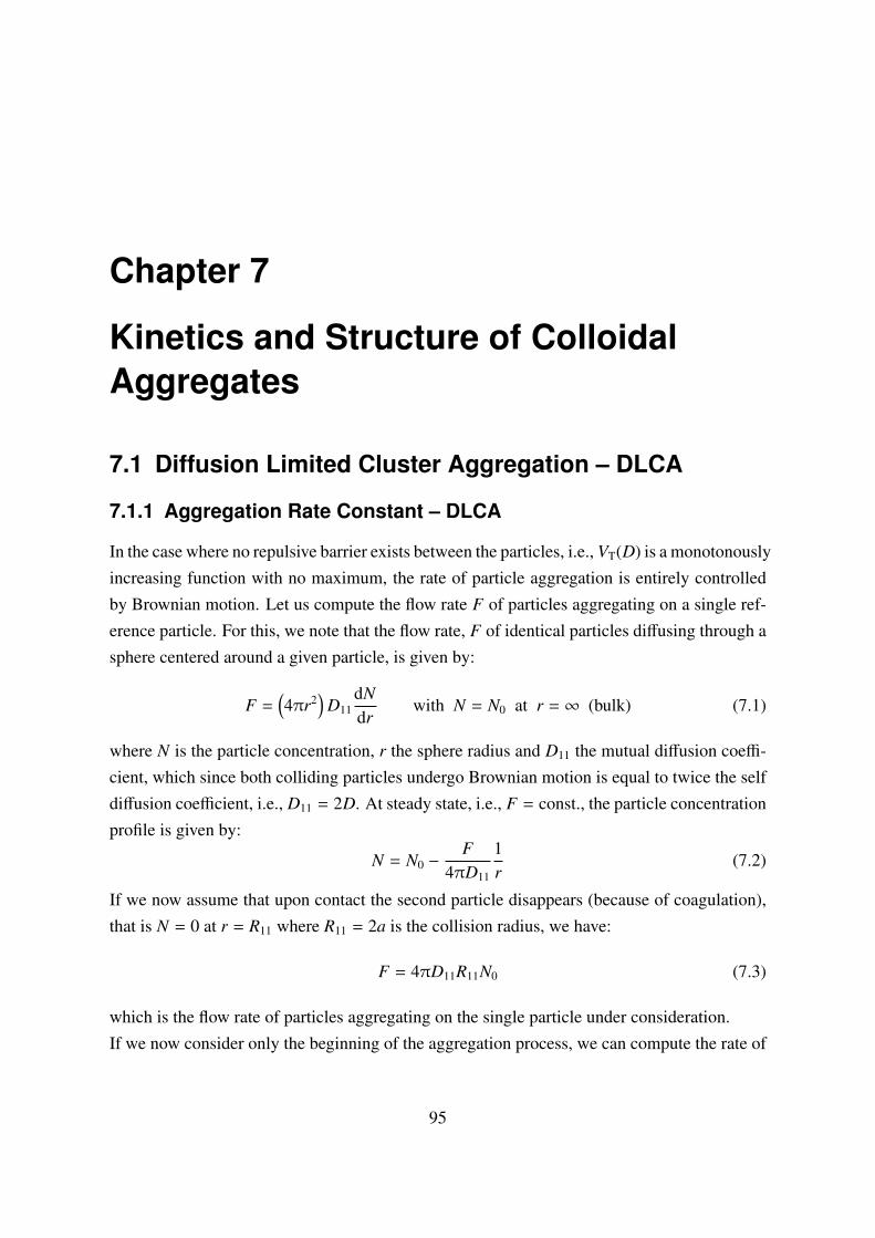
If we now assume that upon contact the second particle disappears (because of coagulation),that is N = 0 at r = R11 where R11 = 2a is the collision radius, we have:
F = 4πD11R11N0 (7.3)
which is the flow rate of particles aggregating on the single particle under consideration.If we now consider only the beginning of the aggregation process, we can compute the rate of
95
CHAPTER 7. KINETICS AND STRUCTURE OF COLLOIDAL AGGREGATES
r
N
N0
2a
decrease of the particle concentration in bulk due to the aggregation process, R0agg as follows:
R0agg = −
12
N0F = −12
4πDR11N20 = −
12β11N2
0 (7.4)
where the factor 1/2 is needed to count each event only once. In the above expression we haveintroduced the aggregation rate constant β11 = 4πD11R11, which plays the same role as thereaction rate constant in a second order kinetics.
In the case of two particles of equal size, a this reduces to:
β11 = 16πDa (7.5)
and using the Stokes-Einstein equation to compute D = kT/(6πηa), where η is the dynamicviscosity of the medium, we obtain:
β11 =83
kTη
(7.6)
which is size independent. In the case of two particles of different radius, Ri and R j, we have:
βi j = 4π(Di + D j
) (Ri + R j
)=
23
kTη
(Ri + R j
) ( 1Ri
+1R j
)(7.7)
It is interesting to investigate the behavior of the aggregation rate constants for particles ofdifferent sizes.
96
CHAPTER 7. KINETICS AND STRUCTURE OF COLLOIDAL AGGREGATES
ai a jβi j
4πDa
a a 4 ⇒ β is size independent
a a/2(
1a + 2
a
) (a + a
2
)= 3 · 3
2 = 4.5
a a/4(
1a + 4
a
) (a + a
4
)= 5 · 5
4 = 6.25
a a/n(
1a + n
a
) (a + a
n
)= (n + 1) (n+1)
n =(n+1)2
n
limn→∞(n+1)2
n = ∞
From the values in the table above it is seen that small/large collisions are more effective thansmall/small or large/large ones.
7.1.2 Cluster Mass Distribution – DLCA
In order to derive the Cluster Mass Distribution (CMD) of the aggregates containing k primaryparticles (or of mass k) we need to consider the following population balance equation, alsoreferred to as Smoluchowski equation:
dNk
dt=
12
k−1∑i=1
βi,k−iNiNk−i − Nk
∞∑i=1
βikNi (7.8)
where Nk is the number concentration of aggregates of size k, and the first term on the r.h.s. rep-resents all possible collisions leading to the formation of an aggregate of mass k, while thesecond is the rate of disappearance of the aggregates of mass k due to aggregation with ag-gregates of any mass. If we now assume that the aggregation rate constant is constant withsize, i.e., βi j = β11 and we sum both sides of the equation above to compute the total aggregateconcentration of any mass, that is
N =
∞∑k=1
Nk (7.9)
we obtain:dNdt
=12β11N2 − β11N2 = −
12β11N2 (7.10)
which integrated with the I.C.: N(t = 0) = N0 leads to:
1N
=1
N0+
12β11t (7.11)
97
CHAPTER 7. KINETICS AND STRUCTURE OF COLLOIDAL AGGREGATES
t
N/N0
tRC
1
0.5
0
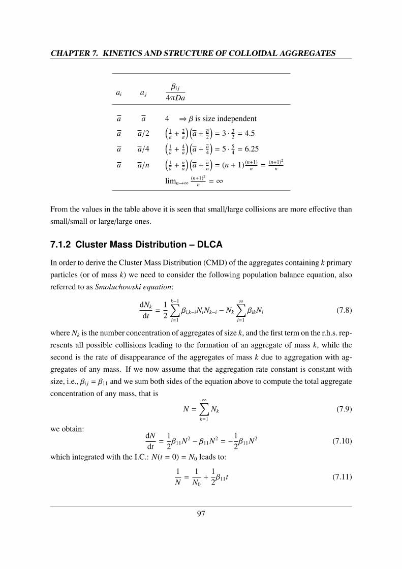
If we define the characteristic time of coagulation or of rapid coagulation, tRC the time neededto half the initial value of aggregates we have:
tRC =2
β11N0=
12πD11R11N0
(7.12)
which for particles of equal size reduces to:
tRC =3η
4kT N0≈
2 × 10¹¹
N0[s] (7.13)
where a water suspension at room temperature has been considered in the latter equation,with N0 in cm−3. As an example, for concentrated colloids of a few percent in solid volume,N0 = 2 × 1014 cm−3 the tRC is in the range of milliseconds.The CMD computed from the Smoluchowski equation is given by:
Nk =N0 (t/τ)k−1
(1 + t/τ)k+1 (7.14)
where time has been made dimensionless using the rapid coagulation time, i.e., τ = tRC.
7.1.3 Role of Aggregate Morphology – DLCA
In order to solve the Smoluchowski equation in the general case where the aggregation rateconstant is size dependent, that is:
βi j =23
kTη
(Ri + R j
) ( 1Ri
+1R j
)(7.15)
98
CHAPTER 7. KINETICS AND STRUCTURE OF COLLOIDAL AGGREGATES
we need to correlate βi j directly to the masses i and j of the two colloiding clusters. Accord-ingly, we need to derive a relation between the size Ri of an aggregate and its mass i, that is tosay something about the structure of the aggregate.
If we consider a solid sphere this relation is simple:
i = ρ43πR3
i , ρ = density (7.16)
which reported on a log-log plot leads to a straight line with slope 1/3. This expressioncan be used in the case of coalescence, where smaller droplets (e.g. of a liquid) aggregate toform a larger drop. In this case, by substituting it in the above equation we get the followingexpression for the coalescence rate constant:
βi j =23
kTη
(i1/3 + j1/3
) (i−1/3 + j−1/3
)(7.17)
Using Monte Carlo simulations and light scattering measurements it has been shown that asimilar straight line is obtained also for the polymer aggregates if we define as aggregate size,Ri the radius of the smallest sphere enveloping the entire cluster. This is the size that wehave tacitely used above in computing the self diffusion coefficient of the fractal using Stokes-Einstein equation.The difference with respect to the solid sphere is that in this case the slope of the straight lineis much larger due to the many voids present in the fractal structure, and equal to 1/df, wheredf is defined as the fractal dimension.
99
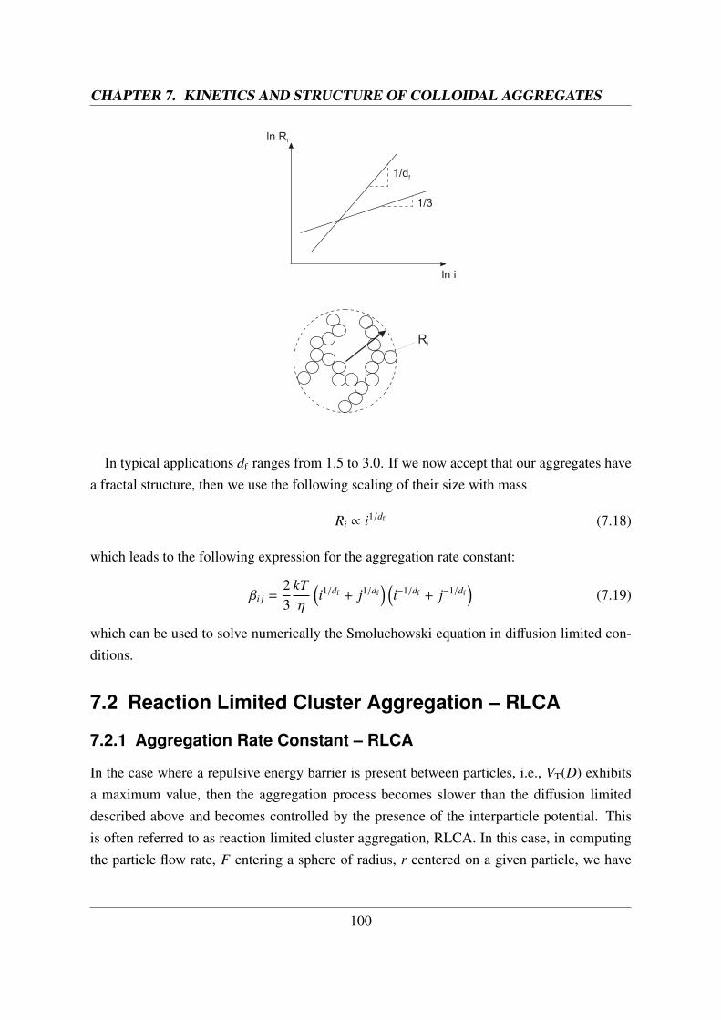
CHAPTER 7. KINETICS AND STRUCTURE OF COLLOIDAL AGGREGATES
1/df
1/3
ln Ri
ln i
Ri
In typical applications df ranges from 1.5 to 3.0. If we now accept that our aggregates havea fractal structure, then we use the following scaling of their size with mass
Ri ∝ i1/df (7.18)
which leads to the following expression for the aggregation rate constant:
βi j =23
kTη
(i1/df + j1/df
) (i−1/df + j−1/df
)(7.19)
which can be used to solve numerically the Smoluchowski equation in diffusion limited con-ditions.
7.2 Reaction Limited Cluster Aggregation – RLCA
7.2.1 Aggregation Rate Constant – RLCA
In the case where a repulsive energy barrier is present between particles, i.e., VT(D) exhibitsa maximum value, then the aggregation process becomes slower than the diffusion limiteddescribed above and becomes controlled by the presence of the interparticle potential. Thisis often referred to as reaction limited cluster aggregation, RLCA. In this case, in computingthe particle flow rate, F entering a sphere of radius, r centered on a given particle, we have
100
CHAPTER 7. KINETICS AND STRUCTURE OF COLLOIDAL AGGREGATES
to consider not only the particle concentration gradient, i.e., brownian diffusion, but also thepotential gradient. The particules are diffusing toward each other while interacting in thepotential field VT(r) whose gradient is producing a force:
FT = −dVT
dr(7.20)
which is contrasted by the friction force given by Stokes law, Ff = Bu, where B = 6πηa
represents the friction coefficient for a sphere of radius, a in a medium with dynamic viscosity,η. The two forces equilibrate each other once the particle reaches the relative terminal velocity,ud so that FT = Ff . This implies a convective flux of particles given by:
Jc = udN = −NB
dVT
dr(7.21)
which superimposes to the diffusion flux:
Jd = −(D11)dNdr
(7.22)
where D11 is the mutual diffusion coefficient of the particles. The flow rate of particlesaggregating on one single particle, F, which at steady state conditions is constant, is given by:
F = −(4πr2
)(Jc + Jd) =
(4πr2
)D11
(dNdr
+NkT
dVT
dr
)(7.23)
where using the Stokes-Einstein equation the friction factor can be represented in terms ofthe diffusion coefficient by B = kT/D11. Using the B.C.: VT = 0, N = N0 at r → ∞, anddN/dr + N
kT dVT/dr = exp(−
VTkT
)d(N exp
(VTkT
))/dr, this equation can be integrated leading to:
N = N0 exp(−
VT
kT
)+
F exp (−VT/kT )4πD11
∫ ∞
rexp
(VT
kT
) drr2 (7.24)
from which, considering N = 0 at r = 2a and D11=2D, we compute:
F = −8πDN0∫ ∞
2aexp (VT/kT ) dr/r2
(7.25)
Note that for VT = 0 we obtain F = 8πDN0(2a), which is the same value computed earlierfor diffusion limited aggregation. Considering the definition of aggregation rate constant,β = F/N, we can conclude that FDLCA/F = βDLCA/β. This is a very important parameter incolloidal science and is usually referred to as the Fuchs or stability ratio, W defined as:
W =βDLCA
β= 2a
∫ ∞
2aexp
(VT
kT
) drr2 (7.26)
101
CHAPTER 7. KINETICS AND STRUCTURE OF COLLOIDAL AGGREGATES
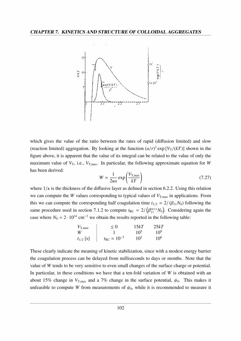
which gives the value of the ratio between the rates of rapid (diffusion limited) and slow(reaction limited) aggregation. By looking at the function (a/r)2 exp [VT/(kT )] shown in thefigure above, it is apparent that the value of its integral can be related to the value of only themaximum value of VT, i.e., VT,max. In particular, the following approximate equation for W
has been derived:W ≈
12κa
exp(VT,max
kT
)(7.27)
where 1/κ is the thickness of the diffusive layer as defined in section 6.2.2. Using this relationwe can compute the W values corresponding to typical values of VT,max in applications. Fromthis we can compute the corresponding half coagulation time t1/2 = 2/ (β11N0) following thesame procedure used in section 7.1.2 to compute tRC = 2/
(βDLCA
11 N0
). Considering again the
case where N0 = 2 · 1014 cm−3 we obtain the results reported in the following table:
VT,max ≤ 0 15kT 25kTW 1 105 109
t1/2 [s] tRC = 10−3 102 106
These clearly indicate the meaning of kinetic stabilization, since with a modest energy barrierthe coagulation process can be delayed from milliseconds to days or months. Note that thevalue of W tends to be very sensitive to even small changes of the surface charge or potential.In particular, in these conditions we have that a ten-fold variation of W is obtained with anabout 15% change in VT,max and a 7% change in the surface potential, ψ0. This makes itunfeasible to compute W from measurements of ψ0, while it is recommended to measure it
102
CHAPTER 7. KINETICS AND STRUCTURE OF COLLOIDAL AGGREGATES
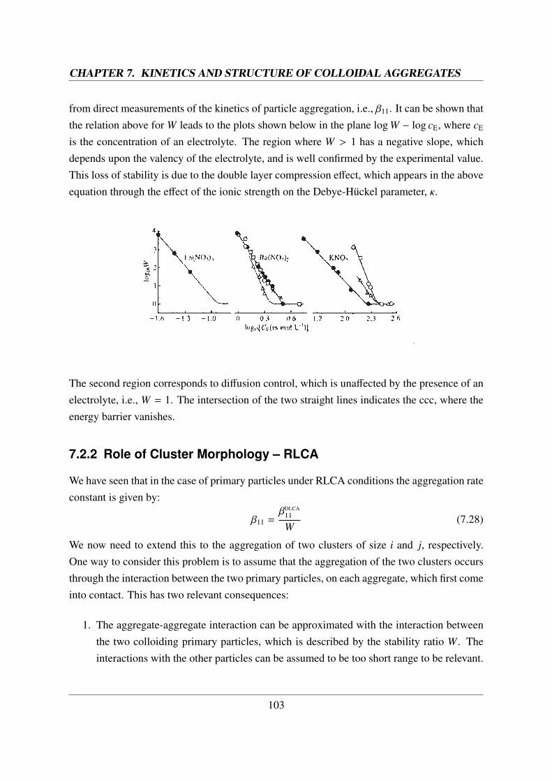
from direct measurements of the kinetics of particle aggregation, i.e., β11. It can be shown thatthe relation above for W leads to the plots shown below in the plane log W − log cE, where cE
is the concentration of an electrolyte. The region where W > 1 has a negative slope, whichdepends upon the valency of the electrolyte, and is well confirmed by the experimental value.This loss of stability is due to the double layer compression effect, which appears in the aboveequation through the effect of the ionic strength on the Debye-Huckel parameter, κ.
The second region corresponds to diffusion control, which is unaffected by the presence of anelectrolyte, i.e., W = 1. The intersection of the two straight lines indicates the ccc, where theenergy barrier vanishes.
7.2.2 Role of Cluster Morphology – RLCA
We have seen that in the case of primary particles under RLCA conditions the aggregation rateconstant is given by:
β11 =βDLCA
11
W(7.28)
We now need to extend this to the aggregation of two clusters of size i and j, respectively.One way to consider this problem is to assume that the aggregation of the two clusters occursthrough the interaction between the two primary particles, on each aggregate, which first comeinto contact. This has two relevant consequences:
1. The aggregate-aggregate interaction can be approximated with the interaction betweenthe two colloiding primary particles, which is described by the stability ratio W. Theinteractions with the other particles can be assumed to be too short range to be relevant.
103
CHAPTER 7. KINETICS AND STRUCTURE OF COLLOIDAL AGGREGATES
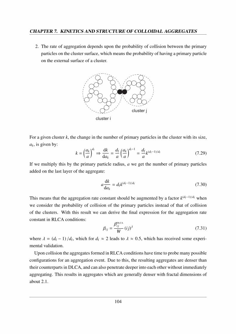
2. The rate of aggregation depends upon the probability of collision between the primaryparticles on the cluster surface, which means the probability of having a primary particleon the external surface of a cluster.
cluster i
cluster j
For a given cluster k, the change in the number of primary particles in the cluster with its size,ak, is given by:
k =
(ak
a
)df
⇒dkdak
=df
a
(ak
a
)df−1=
df
ak(df−1)/df (7.29)
If we multiply this by the primary particle radius, a we get the number of primary particlesadded on the last layer of the aggregate:
adkdak
= dfk(df−1)/df (7.30)
This means that the aggregation rate constant should be augmented by a factor k(df−1)/df whenwe consider the probability of collision of the primary particles instead of that of collisionof the clusters. With this result we can derive the final expression for the aggregation rateconstant in RLCA conditions:
βi j =βDLCA
i j
W(i j)λ (7.31)
where λ = (df − 1) /df , which for df ≈ 2 leads to λ ≈ 0.5, which has received some experi-mental validation.
Upon collision the aggregates formed in RLCA conditions have time to probe many possibleconfigurations for an aggregation event. Due to this, the resulting aggregates are denser thantheir counterparts in DLCA, and can also penetrate deeper into each other without immediatelyaggregating. This results in aggregates which are generally denser with fractal dimensions ofabout 2.1.
104
CHAPTER 7. KINETICS AND STRUCTURE OF COLLOIDAL AGGREGATES
7.2.3 Cluster Mass Distribution – RLCA
In RLCA detailed calculations of the CMD using equation 7.8 with the aggregation rate con-stant shown in equation 7.31 can only be obtained from numerical solutions to the PBE. How-ever, for many aggregation problems in non-sheared colloidal dispersions it has been foundthat the resulting CMD exhibits some general features. Therefore it is possible to developscaling solutions of the PBE, which are often sufficient for approximate purposes. A generalform of the solution for a wide range of aggregation rate constants is given by
Nk (t) = Ak−τ exp (−k/kc) , (7.32)
where A is a normalization constant determined from the conservation of total mass in thesystem and is given by
A =N0kτ−2
c
Γ(2 − τ)(7.33)
where Γ(x) is the gamma function. kc is the time dependent cutoff-mass of the distributionwhich grows with time and determines the kinetics. In RLCA, this growth is exponential, askc(t) = p exp(t/t0), where t0 is a sample dependent time constant. τ is a power-law exponentof the CMD describing the shape of the CMD. In RLCA τ = 1.5 has been found to be areasonable value.
7.3 Comparison of Aggregation Regimes – DLCA vs.RLCA
7.3.1 Aggregation Rate Constant – DLCA vs. RLCA
We now compare the aggregation rate constants of the two aggregation regimes, DLCA andRLCA. The general kernel valid for the two regimes can be written as
βi j = βDLCA11 W−1Bi jPi j with
βDLCA11 = 8kT/(3η)
W =βDLCA
11
β11
Bi j =14
(i−1/df + j−1/df
) (i1/df + j1/df
)Pi j = (i j)λ ,with λ = 0 in DLCA and λ ∼ 0.5 in RLCA,
(7.34)
105
CHAPTER 7. KINETICS AND STRUCTURE OF COLLOIDAL AGGREGATES
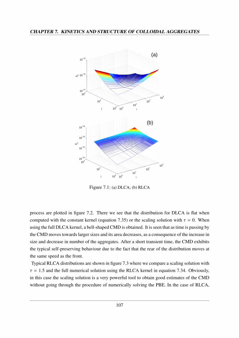
Most important for the aggregation kinetics is the aggregation rate of equal sized aggregatesβii as a function of aggregate mass i. Therefore the parameter λ is extremely important for thekinetics as it dominates this function, as is displayed below.
In DLCA, as discussed before, W ≈ 1 and λ = 0. On the other hand, in RLCA W is largeand λ ≈ 0.5, therefore exhibiting a strong mass dependence of βi j. In summary, in DLCA theaggregation of big with small aggregates is favored and the aggregation rate of equal sizedaggregates is independent of the aggregate mass, whereas in RLCA big clusters preferablyaggregate with big ones such that the aggregation rate of equal sized aggregates strongly in-creases with the aggregate mass. This is reflected by the aggregation rate constant values βi j,shown in figure 7.1 as a function of the aggregate masses i and j in figure 7.1 for the aggrega-tion regimes DLCA and RLCA.
7.3.2 Cluster Mass Distribution – DLCA vs. RLCA
The mathematical formulation of the cluster mass distributions in DLCA and RLCA has beenpresented above. The equations were for DLCA
Nk =N0 (t/τ)k−1
(1 + t/τ)k+1 (7.35)
and for RLCA
Nk (t) =N0kτ−2
c
Γ(2 − τ)k−τ exp (−k/kc) , (7.36)
The last equation can be shown to give identical results to the CMD for DLCA (equation7.35) if τ = 0 is chosen. The different shapes of CMD that are obtained during the aggregation
106
CHAPTER 7. KINETICS AND STRUCTURE OF COLLOIDAL AGGREGATES
100
101
102
103
100
102
104
10−17
10−16
10−15
i j
β ij
(a)
100
101
102
103
100
102
104
10−24
10−22
10−20
10−18
i j
β ij
(b)
Figure 7.1: (a) DLCA; (b) RLCA
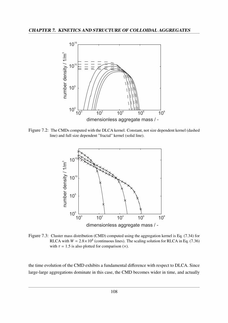
process are plotted in figure 7.2. There we see that the distribution for DLCA is flat whencomputed with the constant kernel (equation 7.35) or the scaling solution with τ = 0. Whenusing the full DLCA kernel, a bell-shaped CMD is obtained. It is seen that as time is passing bythe CMD moves towards larger sizes and its area decreases, as a consequence of the increase insize and decrease in number of the aggregates. After a short transient time, the CMD exhibitsthe typical self-preserving behaviour due to the fact that the rear of the distribution moves atthe same speed as the front.Typical RLCA distributions are shown in figure 7.3 where we compare a scaling solution withτ = 1.5 and the full numerical solution using the RLCA kernel in equation 7.34. Obviously,in this case the scaling solution is a very powerful tool to obtain good estimates of the CMDwithout going through the procedure of numerically solving the PBE. In the case of RLCA,
107
CHAPTER 7. KINETICS AND STRUCTURE OF COLLOIDAL AGGREGATES
100
102
104
106
10810
0
105
1010
1015
num
ber
density
/1/m
3
dimensionless aggregate mass / -
Figure 7.2: The CMDs computed with the DLCA kernel. Constant, not size dependent kernel (dashedline) and full size dependent ”fractal” kernel (solid line).
num
ber
density
/1/m
3
100
105
1010
1015
100
102
104
106
108
dimensionless aggregate mass / -
Figure 7.3: Cluster mass distribution (CMD) computed using the aggregation kernel is Eq. (7.34) forRLCA with W = 2.8×10⁴ (continuous lines). The scaling solution for RLCA in Eq. (7.36)with τ = 1.5 is also plotted for comparison (×).
the time evolution of the CMD exhibits a fundamental difference with respect to DLCA. Sincelarge-large aggregations dominate in this case, the CMD becomes wider in time, and actually
108
CHAPTER 7. KINETICS AND STRUCTURE OF COLLOIDAL AGGREGATES
primary particles remain present in the system up to large aggregation times. The CMD doesnot exhibit the typical bell shape which causes often problems in the technology.
7.3.3 Aggregate Morphology – DLCA vs. RLCA
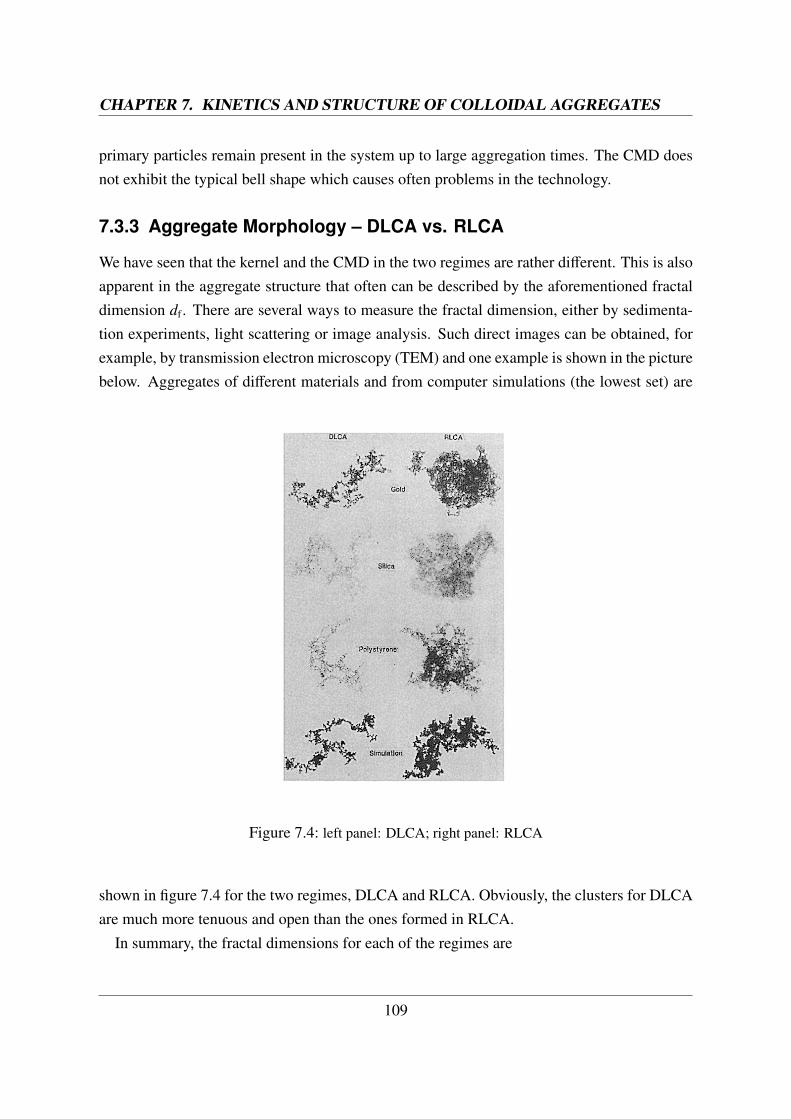
We have seen that the kernel and the CMD in the two regimes are rather different. This is alsoapparent in the aggregate structure that often can be described by the aforementioned fractaldimension df . There are several ways to measure the fractal dimension, either by sedimenta-tion experiments, light scattering or image analysis. Such direct images can be obtained, forexample, by transmission electron microscopy (TEM) and one example is shown in the picturebelow. Aggregates of different materials and from computer simulations (the lowest set) are
Figure 7.4: left panel: DLCA; right panel: RLCA
shown in figure 7.4 for the two regimes, DLCA and RLCA. Obviously, the clusters for DLCAare much more tenuous and open than the ones formed in RLCA.
In summary, the fractal dimensions for each of the regimes are
109
CHAPTER 7. KINETICS AND STRUCTURE OF COLLOIDAL AGGREGATES
Fractal relation: R ∼ i1/df
Regime Fractal dimension df
DLCA 1.6 − 1.9RLCA 2.0 − 2.2
7.3.4 Comparison to Experimental Data
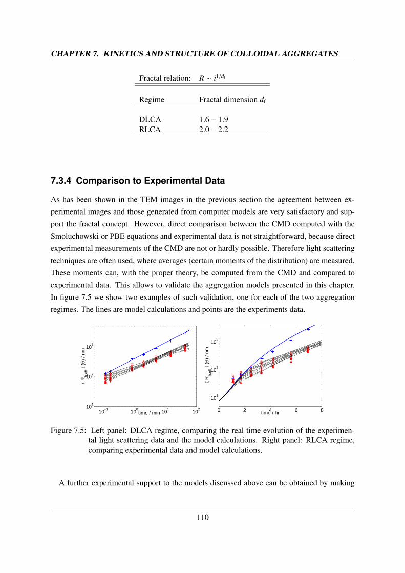
As has been shown in the TEM images in the previous section the agreement between ex-perimental images and those generated from computer models are very satisfactory and sup-port the fractal concept. However, direct comparison between the CMD computed with theSmoluchowski or PBE equations and experimental data is not straightforward, because directexperimental measurements of the CMD are not or hardly possible. Therefore light scatteringtechniques are often used, where averages (certain moments of the distribution) are measured.These moments can, with the proper theory, be computed from the CMD and compared toexperimental data. This allows to validate the aggregation models presented in this chapter.In figure 7.5 we show two examples of such validation, one for each of the two aggregationregimes. The lines are model calculations and points are the experiments data.
10−1
100
101
10210
1
102
103
time / min
⟨ Rh,
eff ⟩
(θ)
/ nm
0 2 4 6 8
101
102
103
time / hr
⟨ R
h,ef
f ⟩ (θ
) / n
m
Figure 7.5: Left panel: DLCA regime, comparing the real time evolution of the experimen-tal light scattering data and the model calculations. Right panel: RLCA regime,comparing experimental data and model calculations.
A further experimental support to the models discussed above can be obtained by making
110
CHAPTER 7. KINETICS AND STRUCTURE OF COLLOIDAL AGGREGATES
the PBE (Eq. 7.8) dimensionless using the following definition for the dimensionless concen-tration of the clusters of mass k and the dimensionless time:
φk =Nk
N0(7.37)
τ = N0βDLCA11
tW
(7.38)
where N0 is the initial number of primary particles, W the Fuchs stability ratio and βDLCA11 the
primary particle aggregation rate constant in DLCA conditions as defined by equation 7.34.Thus, the following dimensionless PBE is obtained from equations 7.8 and 7.34.
dφk
dτ=
12
k−1∑i=1
Bi,k−iPi,k−iφiφk−i − φk
∞∑i=1
Bi,kPi,kφi (7.39)
with initial conditions: φ0 = 1, φk = 0 for k ≥ 0 .
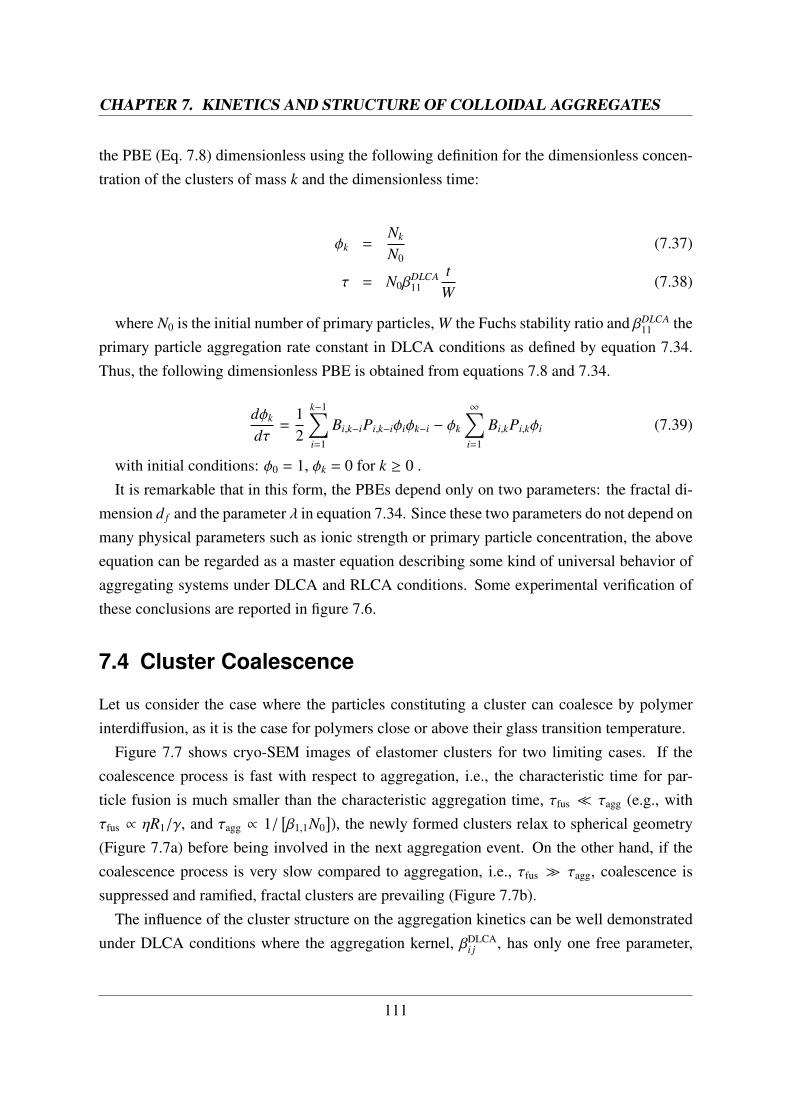
It is remarkable that in this form, the PBEs depend only on two parameters: the fractal di-mension d f and the parameter λ in equation 7.34. Since these two parameters do not depend onmany physical parameters such as ionic strength or primary particle concentration, the aboveequation can be regarded as a master equation describing some kind of universal behavior ofaggregating systems under DLCA and RLCA conditions. Some experimental verification ofthese conclusions are reported in figure 7.6.
7.4 Cluster Coalescence
Let us consider the case where the particles constituting a cluster can coalesce by polymerinterdiffusion, as it is the case for polymers close or above their glass transition temperature.
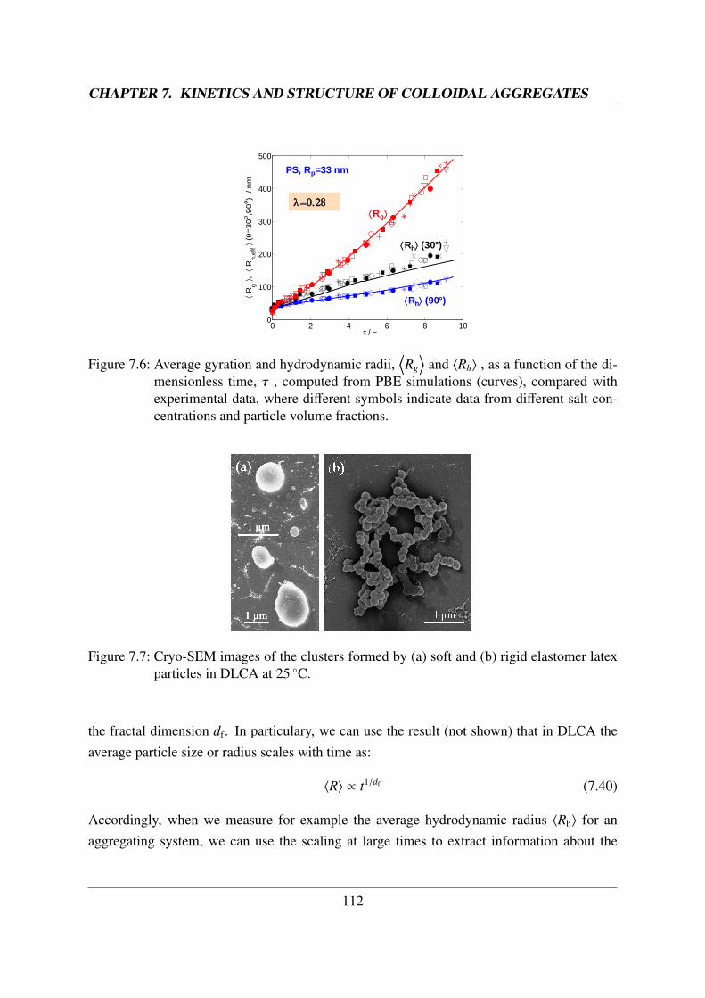
Figure 7.7 shows cryo-SEM images of elastomer clusters for two limiting cases. If thecoalescence process is fast with respect to aggregation, i.e., the characteristic time for par-ticle fusion is much smaller than the characteristic aggregation time, τfus � τagg (e.g., withτfus ∝ ηR1/γ, and τagg ∝ 1/
[β1,1N0
]), the newly formed clusters relax to spherical geometry
(Figure 7.7a) before being involved in the next aggregation event. On the other hand, if thecoalescence process is very slow compared to aggregation, i.e., τfus � τagg, coalescence issuppressed and ramified, fractal clusters are prevailing (Figure 7.7b).
The influence of the cluster structure on the aggregation kinetics can be well demonstratedunder DLCA conditions where the aggregation kernel, βDLCA
i j , has only one free parameter,
111
CHAPTER 7. KINETICS AND STRUCTURE OF COLLOIDAL AGGREGATES
0 2 4 6 8 100
100
200
300
400
500
τ / −
⟨ R
g ⟩
, ⟨
Rh
,eff ⟩
(θ=
30
o,9
0o)
/ n
m
Rh (90°)
Rh (30°)
Rg
PS, Rp=33 nm
Figure 7.6: Average gyration and hydrodynamic radii,⟨Rg
⟩and 〈Rh〉 , as a function of the di-
mensionless time, τ , computed from PBE simulations (curves), compared withexperimental data, where different symbols indicate data from different salt con-centrations and particle volume fractions.
1 µm
1 µm
(a)
1 µm
(b)
Figure 7.7: Cryo-SEM images of the clusters formed by (a) soft and (b) rigid elastomer latexparticles in DLCA at 25 ◦C.
the fractal dimension df . In particulary, we can use the result (not shown) that in DLCA theaverage particle size or radius scales with time as:
〈R〉 ∝ t1/df (7.40)
Accordingly, when we measure for example the average hydrodynamic radius 〈Rh〉 for anaggregating system, we can use the scaling at large times to extract information about the
112
CHAPTER 7. KINETICS AND STRUCTURE OF COLLOIDAL AGGREGATES
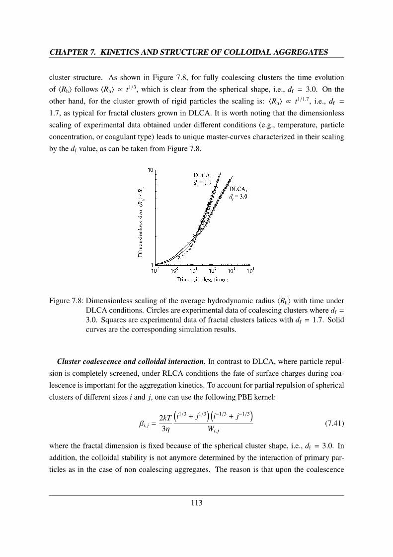
cluster structure. As shown in Figure 7.8, for fully coalescing clusters the time evolutionof 〈Rh〉 follows 〈Rh〉 ∝ t1/3, which is clear from the spherical shape, i.e., df = 3.0. On theother hand, for the cluster growth of rigid particles the scaling is: 〈Rh〉 ∝ t1/1.7, i.e., df =
1.7, as typical for fractal clusters grown in DLCA. It is worth noting that the dimensionlessscaling of experimental data obtained under different conditions (e.g., temperature, particleconcentration, or coagulant type) leads to unique master-curves characterized in their scalingby the df value, as can be taken from Figure 7.8.
Figure 7.8: Dimensionless scaling of the average hydrodynamic radius 〈Rh〉 with time underDLCA conditions. Circles are experimental data of coalescing clusters where df =
3.0. Squares are experimental data of fractal clusters latices with df = 1.7. Solidcurves are the corresponding simulation results.
Cluster coalescence and colloidal interaction. In contrast to DLCA, where particle repul-sion is completely screened, under RLCA conditions the fate of surface charges during coa-lescence is important for the aggregation kinetics. To account for partial repulsion of sphericalclusters of different sizes i and j, one can use the following PBE kernel:
βi, j =2kT3η
(i1/3 + j1/3
) (i−1/3 + j−1/3
)Wi, j
(7.41)
where the fractal dimension is fixed because of the spherical cluster shape, i.e., df = 3.0. Inaddition, the colloidal stability is not anymore determined by the interaction of primary par-ticles as in the case of non coalescing aggregates. The reason is that upon the coalescence
113
CHAPTER 7. KINETICS AND STRUCTURE OF COLLOIDAL AGGREGATES
process on one hand the total polymer surface decreases, thus leading to more stable disper-sions, but on the other hand some of the surface changes may be entrapped inside the newlyformed particles thus having a destabilizing effect.
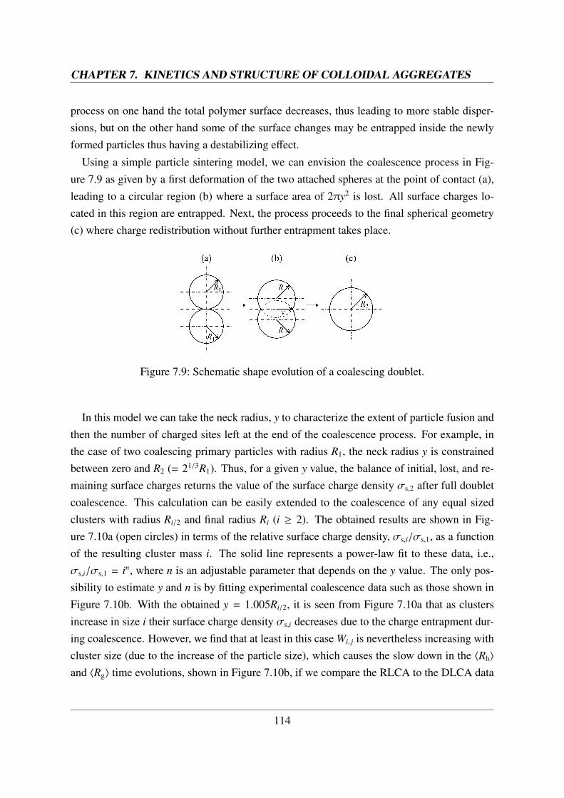
Using a simple particle sintering model, we can envision the coalescence process in Fig-ure 7.9 as given by a first deformation of the two attached spheres at the point of contact (a),leading to a circular region (b) where a surface area of 2πy2 is lost. All surface charges lo-cated in this region are entrapped. Next, the process proceeds to the final spherical geometry(c) where charge redistribution without further entrapment takes place.
Figure 7.9: Schematic shape evolution of a coalescing doublet.
In this model we can take the neck radius, y to characterize the extent of particle fusion andthen the number of charged sites left at the end of the coalescence process. For example, inthe case of two coalescing primary particles with radius R1, the neck radius y is constrainedbetween zero and R2 (= 21/3R1). Thus, for a given y value, the balance of initial, lost, and re-maining surface charges returns the value of the surface charge density σs,2 after full doubletcoalescence. This calculation can be easily extended to the coalescence of any equal sizedclusters with radius Ri/2 and final radius Ri (i ≥ 2). The obtained results are shown in Fig-ure 7.10a (open circles) in terms of the relative surface charge density, σs,i/σs,1, as a functionof the resulting cluster mass i. The solid line represents a power-law fit to these data, i.e.,σs,i/σs,1 = in, where n is an adjustable parameter that depends on the y value. The only pos-sibility to estimate y and n is by fitting experimental coalescence data such as those shown inFigure 7.10b. With the obtained y = 1.005Ri/2, it is seen from Figure 7.10a that as clustersincrease in size i their surface charge density σs,i decreases due to the charge entrapment dur-ing coalescence. However, we find that at least in this case Wi, j is nevertheless increasing withcluster size (due to the increase of the particle size), which causes the slow down in the 〈Rh〉
and 〈Rg〉 time evolutions, shown in Figure 7.10b, if we compare the RLCA to the DLCA data
114
CHAPTER 7. KINETICS AND STRUCTURE OF COLLOIDAL AGGREGATES
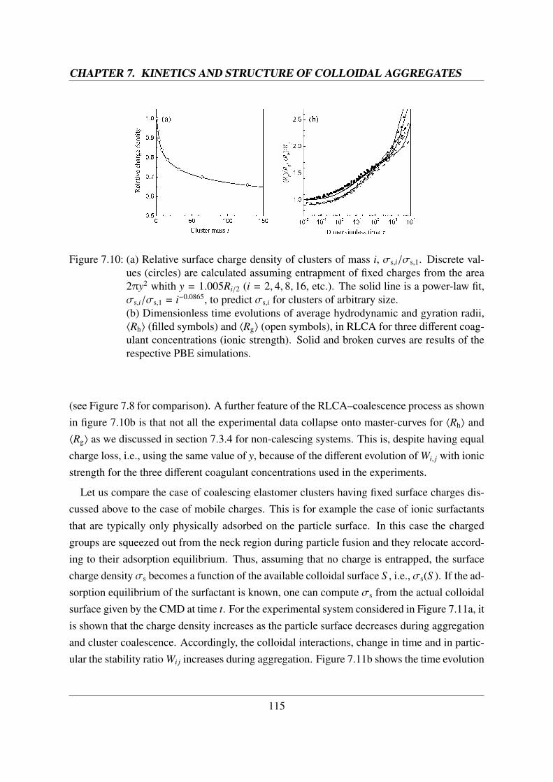
Figure 7.10: (a) Relative surface charge density of clusters of mass i, σs,i/σs,1. Discrete val-ues (circles) are calculated assuming entrapment of fixed charges from the area2πy2 whith y = 1.005Ri/2 (i = 2, 4, 8, 16, etc.). The solid line is a power-law fit,σs,i/σs,1 = i−0.0865, to predict σs,i for clusters of arbitrary size.(b) Dimensionless time evolutions of average hydrodynamic and gyration radii,〈Rh〉 (filled symbols) and 〈Rg〉 (open symbols), in RLCA for three different coag-ulant concentrations (ionic strength). Solid and broken curves are results of therespective PBE simulations.
(see Figure 7.8 for comparison). A further feature of the RLCA–coalescence process as shownin figure 7.10b is that not all the experimental data collapse onto master-curves for 〈Rh〉 and〈Rg〉 as we discussed in section 7.3.4 for non-calescing systems. This is, despite having equalcharge loss, i.e., using the same value of y, because of the different evolution of Wi, j with ionicstrength for the three different coagulant concentrations used in the experiments.
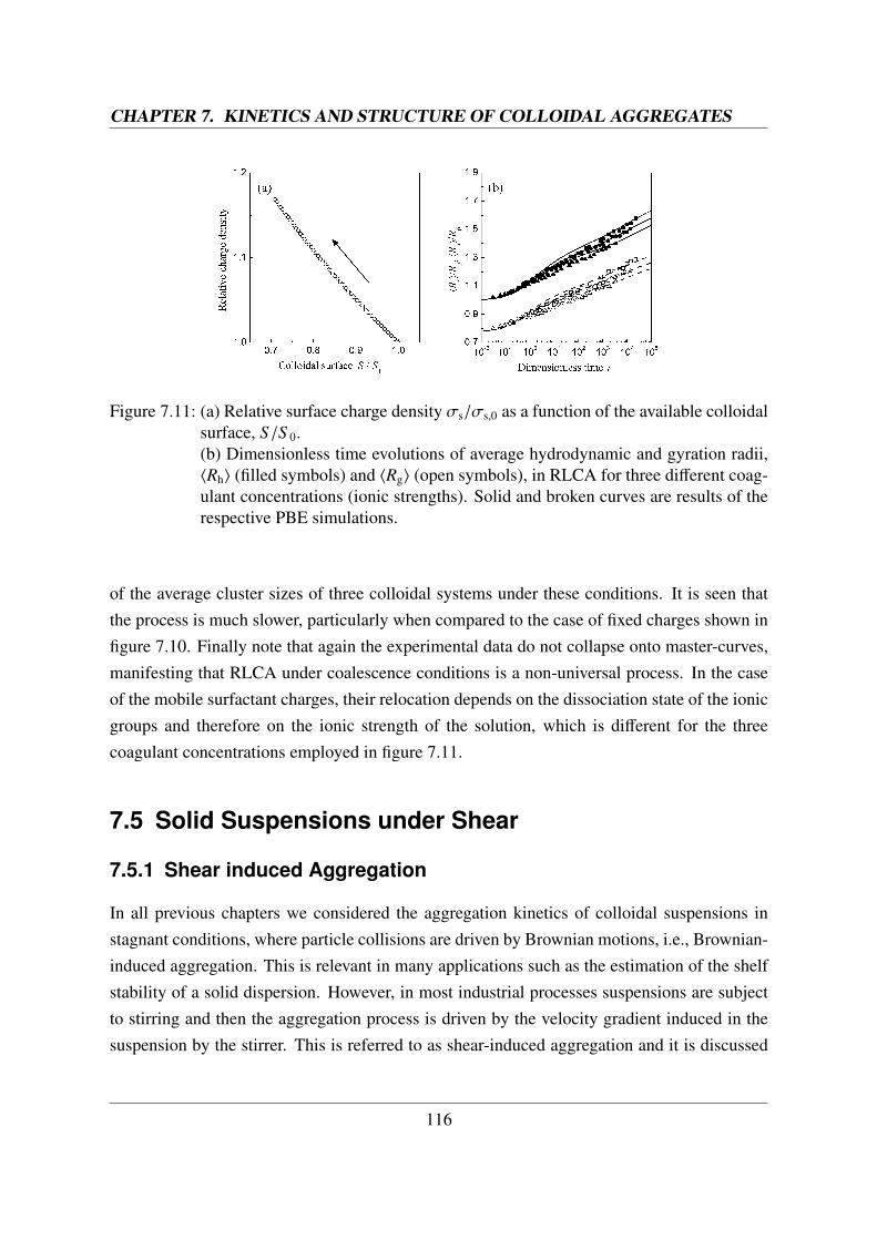
Let us compare the case of coalescing elastomer clusters having fixed surface charges dis-cussed above to the case of mobile charges. This is for example the case of ionic surfactantsthat are typically only physically adsorbed on the particle surface. In this case the chargedgroups are squeezed out from the neck region during particle fusion and they relocate accord-ing to their adsorption equilibrium. Thus, assuming that no charge is entrapped, the surfacecharge density σs becomes a function of the available colloidal surface S , i.e., σs(S ). If the ad-sorption equilibrium of the surfactant is known, one can compute σs from the actual colloidalsurface given by the CMD at time t. For the experimental system considered in Figure 7.11a, itis shown that the charge density increases as the particle surface decreases during aggregationand cluster coalescence. Accordingly, the colloidal interactions, change in time and in partic-ular the stability ratio Wi j increases during aggregation. Figure 7.11b shows the time evolution
115
CHAPTER 7. KINETICS AND STRUCTURE OF COLLOIDAL AGGREGATES
Figure 7.11: (a) Relative surface charge density σs/σs,0 as a function of the available colloidalsurface, S/S 0.(b) Dimensionless time evolutions of average hydrodynamic and gyration radii,〈Rh〉 (filled symbols) and 〈Rg〉 (open symbols), in RLCA for three different coag-ulant concentrations (ionic strengths). Solid and broken curves are results of therespective PBE simulations.
of the average cluster sizes of three colloidal systems under these conditions. It is seen thatthe process is much slower, particularly when compared to the case of fixed charges shown infigure 7.10. Finally note that again the experimental data do not collapse onto master-curves,manifesting that RLCA under coalescence conditions is a non-universal process. In the caseof the mobile surfactant charges, their relocation depends on the dissociation state of the ionicgroups and therefore on the ionic strength of the solution, which is different for the threecoagulant concentrations employed in figure 7.11.
7.5 Solid Suspensions under Shear
7.5.1 Shear induced Aggregation
In all previous chapters we considered the aggregation kinetics of colloidal suspensions instagnant conditions, where particle collisions are driven by Brownian motions, i.e., Brownian-induced aggregation. This is relevant in many applications such as the estimation of the shelfstability of a solid dispersion. However, in most industrial processes suspensions are subjectto stirring and then the aggregation process is driven by the velocity gradient induced in thesuspension by the stirrer. This is referred to as shear-induced aggregation and it is discussed
116
CHAPTER 7. KINETICS AND STRUCTURE OF COLLOIDAL AGGREGATES
in the following.
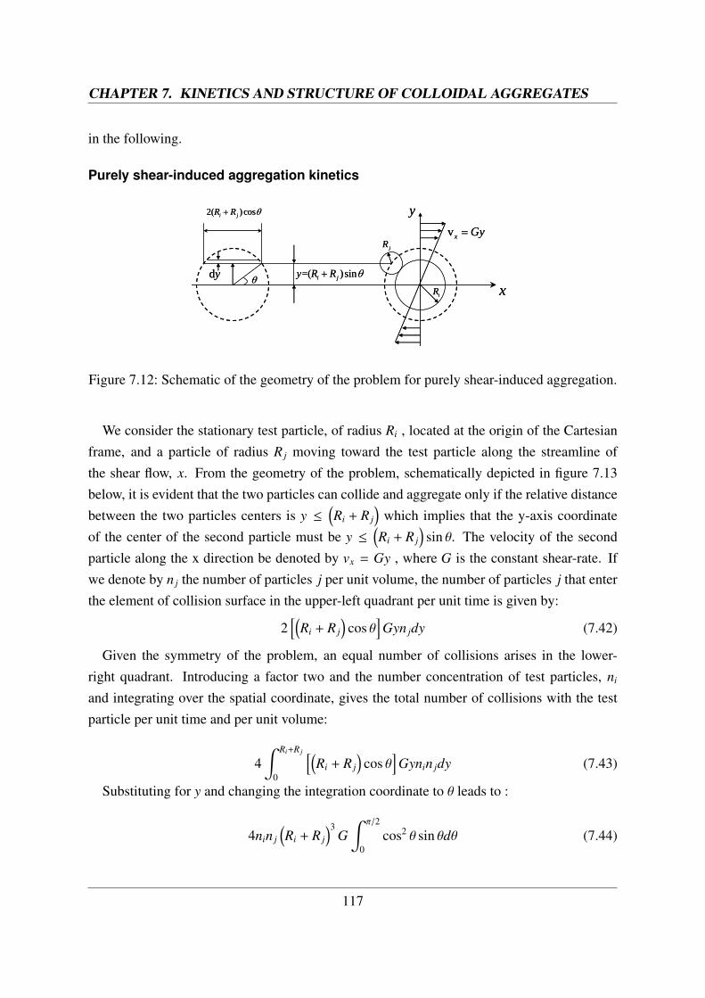
Purely shear-induced aggregation kinetics
dy
2( )cosi jR R
=( )sini jy R R
x
y
iR
jRvx Gy
dy
2( )cosi jR R
=( )sini jy R R
x
y
iR
jRvx Gy
Figure 7.12: Schematic of the geometry of the problem for purely shear-induced aggregation.
We consider the stationary test particle, of radius Ri , located at the origin of the Cartesianframe, and a particle of radius R j moving toward the test particle along the streamline ofthe shear flow, x. From the geometry of the problem, schematically depicted in figure 7.13below, it is evident that the two particles can collide and aggregate only if the relative distancebetween the two particles centers is y ≤
(Ri + R j
)which implies that the y-axis coordinate
of the center of the second particle must be y ≤(Ri + R j
)sin θ. The velocity of the second
particle along the x direction be denoted by vx = Gy , where G is the constant shear-rate. Ifwe denote by n j the number of particles j per unit volume, the number of particles j that enterthe element of collision surface in the upper-left quadrant per unit time is given by:
2[(
Ri + R j
)cos θ
]Gyn jdy (7.42)
Given the symmetry of the problem, an equal number of collisions arises in the lower-right quadrant. Introducing a factor two and the number concentration of test particles, ni
and integrating over the spatial coordinate, gives the total number of collisions with the testparticle per unit time and per unit volume:
4∫ Ri+R j
0
[(Ri + R j
)cos θ
]Gynin jdy (7.43)
Substituting for y and changing the integration coordinate to θ leads to :
4nin j
(Ri + R j
)3G
∫ π/2
0cos2 θ sin θdθ (7.44)
117
CHAPTER 7. KINETICS AND STRUCTURE OF COLLOIDAL AGGREGATES
from which the collision frequency per unit volume follows as:
β11 =32R3G
3(7.45)
This result, which was derived for the first time by M. von Smoluchowski in the eventfulyear 1917, shows that the rate of shear-induced aggregation is proportional to the shear rateand to third power of the sum of the particle radii. This strong dependence on the particlesize is what renders shear aggregation faster than Brownian aggregation for sufficiently largeparticles.
The above β11 expression is valid under laminar conditions, seldom encountered in indus-trial units that typically operate under turbulent conditions. In the presence of turbulence, suchdependency is still valid, provided that G is replaced by an average shear rate that can be cal-culated from the average energy dissipation rate of the turbulent flow, ε. This approximation isvalid in the case where the aggregates are smaller than the Kolmogorof vortexes, within whichthe laminar flow prevails with shear equal to G = (ε/ν)0.5 , where ν is the kinematic viscosityof the disperse medium.
Generalization to DLVO-interacting Brownian particles in shear flow
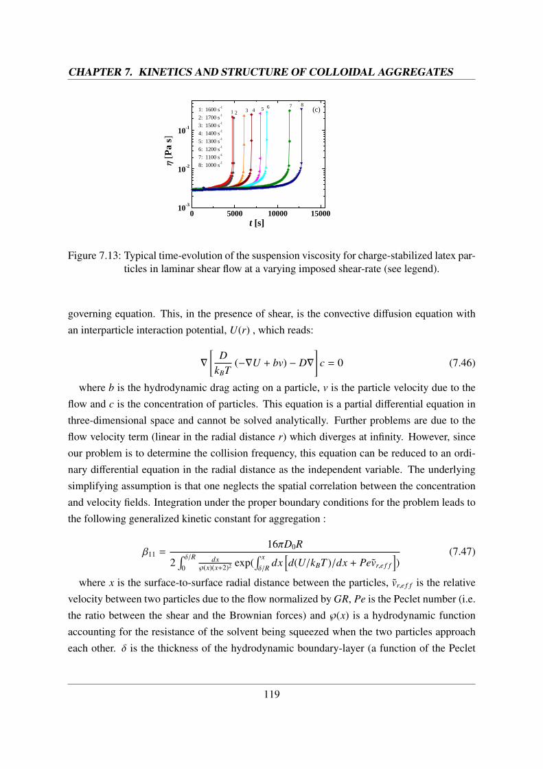
The Smoluchowski result for purely shear-induced aggregation kinetics is valid under therestrictive hypotheses that the particles are non-Brownian and non-interacting. The latter hy-pothesis means that the particles are treated as hard spheres which stick upon collision. Theshear-induced aggregation kinetics of Brownian particles which do interact (typically with asuperposition of van der Waals attraction and electric double layer repulsion) is a more com-plicated problem. The interplay between shear and interactions in this case gives rise to aninteresting phenomenology: a colloidal suspension which is completely stable under stagnantconditions (owing to charge-stabilization) can be made to aggregate under the imposition ofshear flow, with the result that the rheological properties of the suspension may change dramat-ically. A typical situation is depicted in the Figure below, where, after a lag-time or inductionperiod within which it remains constant, the viscosity suddenly undergoes a very sharp upturnand eventually results in the overload of the shearing device, and the system turns into solid-like upon cessation of flow. Furthermore, the duration of the lag-time correlates exponentiallywith the applied shear-rate, in the sense that the lag-time before the viscosity upturn decreasesexponentially upon increasing the shear rate.
The difficulty of treating this general case is related to the mathematical complexity of the
118
CHAPTER 7. KINETICS AND STRUCTURE OF COLLOIDAL AGGREGATES
0 5000 10000 1500010-3
10-2
10-1
[P
a s]
t [s]
1: 1600 s-1
2: 1700 s-1
3: 1500 s-1
4: 1400 s-1
5: 1300 s-1
6: 1200 s-1
7: 1100 s-1
8: 1000 s-1
1 2 3 4 5 6 7 8(c)
Figure 7.13: Typical time-evolution of the suspension viscosity for charge-stabilized latex par-ticles in laminar shear flow at a varying imposed shear-rate (see legend).
governing equation. This, in the presence of shear, is the convective diffusion equation withan interparticle interaction potential, U(r) , which reads:
∇
[D
kBT(−∇U + bv) − D∇
]c = 0 (7.46)
where b is the hydrodynamic drag acting on a particle, v is the particle velocity due to theflow and c is the concentration of particles. This equation is a partial differential equation inthree-dimensional space and cannot be solved analytically. Further problems are due to theflow velocity term (linear in the radial distance r) which diverges at infinity. However, sinceour problem is to determine the collision frequency, this equation can be reduced to an ordi-nary differential equation in the radial distance as the independent variable. The underlyingsimplifying assumption is that one neglects the spatial correlation between the concentrationand velocity fields. Integration under the proper boundary conditions for the problem leads tothe following generalized kinetic constant for aggregation :
β11 =16πD0R
2∫ δ/R
0dx
℘(x)(x+2)2 exp(∫ x
δ/Rdx
[d(U/kBT )/dx + Pevr,e f f
])
(7.47)
where x is the surface-to-surface radial distance between the particles, vr,e f f is the relativevelocity between two particles due to the flow normalized by GR, Pe is the Peclet number (i.e.the ratio between the shear and the Brownian forces) and ℘(x) is a hydrodynamic functionaccounting for the resistance of the solvent being squeezed when the two particles approacheach other. δ is the thickness of the hydrodynamic boundary-layer (a function of the Peclet
119
CHAPTER 7. KINETICS AND STRUCTURE OF COLLOIDAL AGGREGATES
number and of the interaction range). This expression is still sufficiently complicated, wherethe integrals need be evaluated numerically. A further simplification can be done by consider-ing the limits of a high interaction potential barrier and moderate Peclet number. Under theseconditions, the previous expression reduces to the following simple relationship:
β11 =
√Pe − (U ′′
m/kBT ) exp (−Um/kBT + 2Pe/3π) (7.48)
where Um is the value of the interaction potential at the maximum of the barrier and U′′
m isthe second derivative evaluated at the maximum. Since the Peclet is proportional to the shearrate (Pe = 3πµGR3/kBT , where µ is the solvent viscosity,kB is Boltzmann’s constant, andT is the absolute temperature) this formula explains the observed exponential dependence ofthe lag-time preceding the viscosity upturn upon the shear-rate in terms of the attempt time(activation delay) for the shear-induced aggregation of particles with a potential barrier. Theexponential scaling with the shear-rate predicted by this formula is in fairly good agreementwith experimental observations.
800 1200 1600103
104
105
G[s-1]
Ch
arac
teri
stic
ag
greg
atio
n ti
me
[s]
800 1200 1600103
104
105
G[s-1]
Ch
arac
teri
stic
ag
greg
atio
n ti
me
[s]
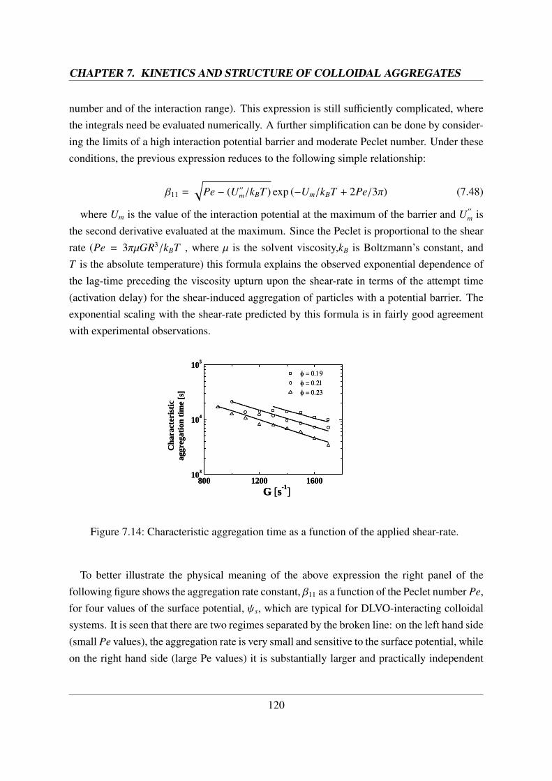
Figure 7.14: Characteristic aggregation time as a function of the applied shear-rate.
To better illustrate the physical meaning of the above expression the right panel of thefollowing figure shows the aggregation rate constant, β11 as a function of the Peclet number Pe,for four values of the surface potential, ψs, which are typical for DLVO-interacting colloidalsystems. It is seen that there are two regimes separated by the broken line: on the left hand side(small Pe values), the aggregation rate is very small and sensitive to the surface potential, whileon the right hand side (large Pe values) it is substantially larger and practically independent
120
CHAPTER 7. KINETICS AND STRUCTURE OF COLLOIDAL AGGREGATES
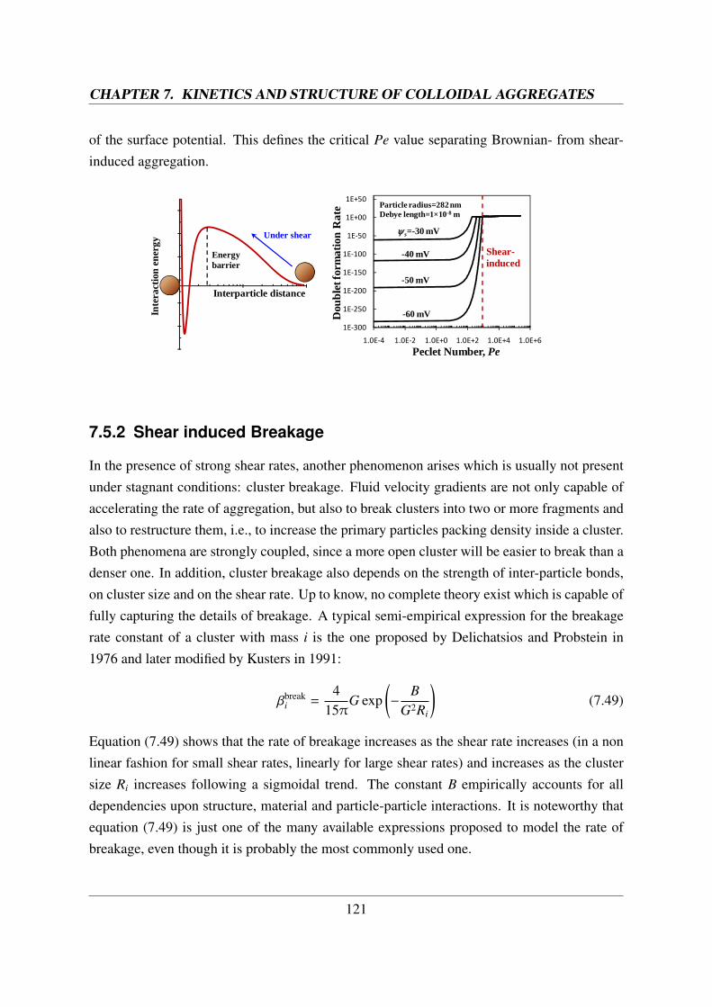
of the surface potential. This defines the critical Pe value separating Brownian- from shear-induced aggregation.
Inte
ract
ion
en
ergy
Interparticle distance
Energy barrier
Under shear
1E‐300
1E‐250
1E‐200
1E‐150
1E‐100
1E‐50
1E+00
1E+50
1.0E‐4 1.0E‐2 1.0E+0 1.0E+2 1.0E+4 1.0E+6D
oub
let f
orm
atio
n R
ate
Peclet Number, Pe
s=-30 mV
-40 mV
Particle radius=282 nmDebye length=1×10⁻⁸ m
-50 mV
-60 mV
Shear-induced
7.5.2 Shear induced Breakage
In the presence of strong shear rates, another phenomenon arises which is usually not presentunder stagnant conditions: cluster breakage. Fluid velocity gradients are not only capable ofaccelerating the rate of aggregation, but also to break clusters into two or more fragments andalso to restructure them, i.e., to increase the primary particles packing density inside a cluster.Both phenomena are strongly coupled, since a more open cluster will be easier to break than adenser one. In addition, cluster breakage also depends on the strength of inter-particle bonds,on cluster size and on the shear rate. Up to know, no complete theory exist which is capable offully capturing the details of breakage. A typical semi-empirical expression for the breakagerate constant of a cluster with mass i is the one proposed by Delichatsios and Probstein in1976 and later modified by Kusters in 1991:
βbreaki =
415π
G exp(−
BG2Ri
)(7.49)
Equation (7.49) shows that the rate of breakage increases as the shear rate increases (in a nonlinear fashion for small shear rates, linearly for large shear rates) and increases as the clustersize Ri increases following a sigmoidal trend. The constant B empirically accounts for alldependencies upon structure, material and particle-particle interactions. It is noteworthy thatequation (7.49) is just one of the many available expressions proposed to model the rate ofbreakage, even though it is probably the most commonly used one.
121
CHAPTER 7. KINETICS AND STRUCTURE OF COLLOIDAL AGGREGATES
One of the major difficulties related in the modelling of breakage events is that the rateof breakage is not the only piece of information required to construct a mathematical modelfor coagulation in the presence of shear. In fact, it is necessary to also know the distributionof fragments generated in a breakage event. Unfortunately, it is very difficult to obtain thefragment distribution function both theoretically and experimentally. Usually, either simplebinary breakage or fragmentation of a cluster into a specific number of equal size fragmentsare assumed.
One significant difference between a breakage event and an aggregation event is that break-age is a first order kinetic process, i.e., the rate of breakage is proportional to the first powerto the cluster concentration, while all aggregation mechanisms discussed so far are secondorder kinetic processes, because they require the collision of two clusters. This implies thatthe formulation of population balance equations (PBE) changes substantially when breakageis present. The PBE (equation (7.8)) in the presence of shear can be formulated as follows:
dNk
dt=
12
k−1∑i=1
βi,k−iNiNk−i − Nk
∞∑i=1
βikNi − βbreakk Nk +
∞∑i=k+1
Γk,iβbreaki Ni (7.50)
The last two terms of equation (7.50) provide the contribution due to breakage to the mass bal-ances. The second last term is a mass loss, due to the breakage of clusters with mass k, whilethe last term is a positive contribution due to formation of clusters with mass k generated bythe fragmentation of all clusters with mass i > k. The function Γk,i is the fragment distributionfunction, which is defined as the number of fragments with mass k generated by breaking acluster with mass i.
7.6 Gelation of Colloidal Suspensions
7.6.1 The Gelation Process
During aggregation clusters continuously grow in size. Taking the radius of the smallest sphereenveloping the cluster of mass i as the cluster dimension, Ri, we can compute the cumulativevolume fraction occupied by all clusters, as follows:
φ(t) =∑
i
43πR3
i Ni (7.51)
where Ni is the CMD, for example computed through the PBE (Eq. 7.8). As shown in fig-ure 7.15, φ(t) increases in time reaching values larger than one. This indicates that the system
122
CHAPTER 7. KINETICS AND STRUCTURE OF COLLOIDAL AGGREGATES
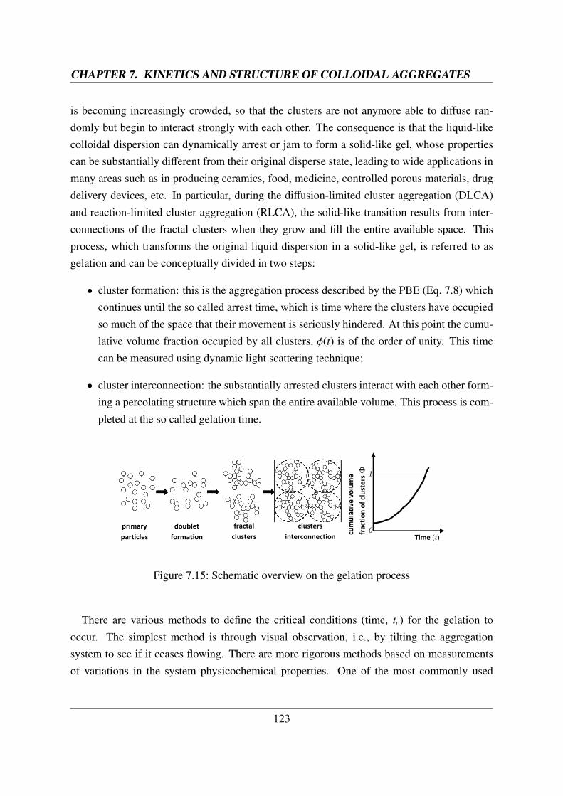
is becoming increasingly crowded, so that the clusters are not anymore able to diffuse ran-domly but begin to interact strongly with each other. The consequence is that the liquid-likecolloidal dispersion can dynamically arrest or jam to form a solid-like gel, whose propertiescan be substantially different from their original disperse state, leading to wide applications inmany areas such as in producing ceramics, food, medicine, controlled porous materials, drugdelivery devices, etc. In particular, during the diffusion-limited cluster aggregation (DLCA)and reaction-limited cluster aggregation (RLCA), the solid-like transition results from inter-connections of the fractal clusters when they grow and fill the entire available space. Thisprocess, which transforms the original liquid dispersion in a solid-like gel, is referred to asgelation and can be conceptually divided in two steps:
• cluster formation: this is the aggregation process described by the PBE (Eq. 7.8) whichcontinues until the so called arrest time, which is time where the clusters have occupiedso much of the space that their movement is seriously hindered. At this point the cumu-lative volume fraction occupied by all clusters, φ(t) is of the order of unity. This timecan be measured using dynamic light scattering technique;
• cluster interconnection: the substantially arrested clusters interact with each other form-ing a percolating structure which span the entire available volume. This process is com-pleted at the so called gelation time.
Time (t) 0
1
cumulative
volume
fraction of clusters
Ф
primary
particles
doublet
formation
fractal
clusters
clusters
interconnection
Figure 7.15: Schematic overview on the gelation process
There are various methods to define the critical conditions (time, tc) for the gelation tooccur. The simplest method is through visual observation, i.e., by tilting the aggregationsystem to see if it ceases flowing. There are more rigorous methods based on measurementsof variations in the system physicochemical properties. One of the most commonly used
123
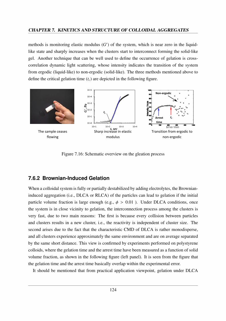
CHAPTER 7. KINETICS AND STRUCTURE OF COLLOIDAL AGGREGATES
methods is monitoring elastic modulus (G′) of the system, which is near zero in the liquid-like state and sharply increases when the clusters start to interconnect forming the solid-likegel. Another technique that can be well used to define the occurrence of gelation is cross-correlation dynamic light scattering, whose intensity indicates the transition of the systemfrom ergodic (liquid-like) to non-ergodic (solid-like). The three methods mentioned above todefine the critical gelation time (tc) are depicted in the following figure.
The sample ceases
flowing
1E+0
1E+1
1E+2
1E+3
1E+4
1E+5
1E+1 1E+2 1E+3 1E+4
G',
Pa
t, sec
tc
Arrest
time
Non‐ergodic
tc
Sharp increase in elastic
modulus
Transition from ergodic to
non‐ergodic
Figure 7.16: Schematic overview on the gleation process
7.6.2 Brownian-Induced Gelation
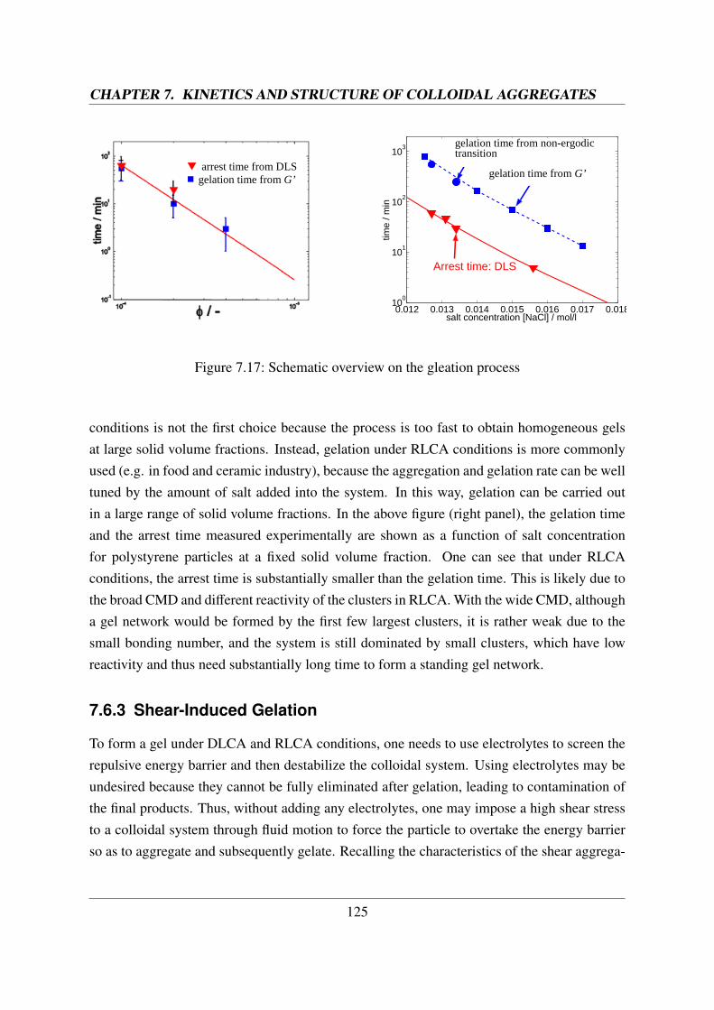
When a colloidal system is fully or partially destabilized by adding electrolytes, the Brownian-induced aggregation (i.e., DLCA or RLCA) of the particles can lead to gelation if the initialparticle volume fraction is large enough (e.g., φ > 0.01 ). Under DLCA conditions, oncethe system is in close vicinity to gelation, the interconnection process among the clusters isvery fast, due to two main reasons: The first is because every collision between particlesand clusters results in a new cluster, i.e., the reactivity is independent of cluster size. Thesecond arises due to the fact that the characteristic CMD of DLCA is rather monodisperse,and all clusters experience approximately the same environment and are on average separatedby the same short distance. This view is confirmed by experiments performed on polystyrenecolloids, where the gelation time and the arrest time have been measured as a function of solidvolume fraction, as shown in the following figure (left panel). It is seen from the figure thatthe gelation time and the arrest time basically overlap within the experimental error.
It should be mentioned that from practical application viewpoint, gelation under DLCA
124
CHAPTER 7. KINETICS AND STRUCTURE OF COLLOIDAL AGGREGATES
0.012 0.013 0.014 0.015 0.016 0.017 0.01810
0
101
102
103
salt concentration [NaCl] / mol/l
time
/ min
Rheology: gelation time
Arrest time: DLS
3D DLS: NE−transition
gelation time from G’
gelation time from non-ergodic transition
RLCA gelation at different salt
concentrations; =0.05; Rp=40 nm
DLCA gelation at different solid
volume fractions; Rp=35 nm
arrest time from DLS gelation time from G’
Figure 7.17: Schematic overview on the gleation process
conditions is not the first choice because the process is too fast to obtain homogeneous gelsat large solid volume fractions. Instead, gelation under RLCA conditions is more commonlyused (e.g. in food and ceramic industry), because the aggregation and gelation rate can be welltuned by the amount of salt added into the system. In this way, gelation can be carried outin a large range of solid volume fractions. In the above figure (right panel), the gelation timeand the arrest time measured experimentally are shown as a function of salt concentrationfor polystyrene particles at a fixed solid volume fraction. One can see that under RLCAconditions, the arrest time is substantially smaller than the gelation time. This is likely due tothe broad CMD and different reactivity of the clusters in RLCA. With the wide CMD, althougha gel network would be formed by the first few largest clusters, it is rather weak due to thesmall bonding number, and the system is still dominated by small clusters, which have lowreactivity and thus need substantially long time to form a standing gel network.
7.6.3 Shear-Induced Gelation
To form a gel under DLCA and RLCA conditions, one needs to use electrolytes to screen therepulsive energy barrier and then destabilize the colloidal system. Using electrolytes may beundesired because they cannot be fully eliminated after gelation, leading to contamination ofthe final products. Thus, without adding any electrolytes, one may impose a high shear stressto a colloidal system through fluid motion to force the particle to overtake the energy barrierso as to aggregate and subsequently gelate. Recalling the characteristics of the shear aggrega-
125
CHAPTER 7. KINETICS AND STRUCTURE OF COLLOIDAL AGGREGATES
tion process discussed in section 7.5.1 and in particular the dependence of the correspondingaggregation rate constant on the Pe number, we can conclude that once the imposed shear ishigh enough, leading to a Pe value in the shear-induced regime, the aggregation will be ex-tremely fast and independent of the DLVO interactions. This occurs for Pe values larger thanthe critical value leading to shear-induced aggregation.
In practical applications, shear-induced gelation can be realized by forcing a colloidal sys-tem to pass through a microchannel (MC) without adding any electrolyte to screen the DLVOinteractions. The left panel of the following figure shows an example of such a device wherethe capillary exhibits a z-shape with retention times in the order of tens of microseconds andpressure in the range of 20 to 120 bar. The intense shear is generated by forcing the col-loidal system to pass through the z-MC under pressure. In general, right after passing throughthe z-MC, the system can be either a Newtonian liquid or a viscous non-Newtonian liquid orsolid-like gel, depending on how many clusters have been generated, which in turn dependson the shear rate, the particle volume fraction and size. One can speculate that if a sufficientamount of clusters is formed in the capillary, gelation occurs and at the MC outlet we have asolid gel having diameter similar to that of the connecting tube. If the conditions for gelationare not reached then the exiting liquid suspension is composed of two distinct classes of clus-ters: Class 1, constituted mainly of primary particles, and at most some dimers and trimers,and Class 2, constituted of large clusters (or gels) with sizes at least two orders of magnitudelarger than that of the primary particles. It is remarkable that clusters with intermediate sizeare negligible. These two classes can in fact be easily isolated using a 5 µm-opening filter.Such a bimodal CMD is rather different from the CMDs which are typically obtained underDLCA or RLCA conditions, and it is indeed difficult to be explained on physical ground.
On the other hand, when one thinks to the formation of macroscopic pieces of coagulumwhich is often observed in suspension/emulsion reactors and coagulators, this can certainlynot be regarded as an academic curiosity. One possible explanation can be offered by referringagain to the critical transition from Brownian to shear induced aggregation (Pe is alreadyabove the critical Pe!). Since the Pe number depends upon the third power of the aggregatesize, one can speculate that if in an otherwise stable suspension (i.e., under very slow Brownianaggregation) a very few doublets or triplets are formed (for whatever reason) they might enterthe shear-induced aggregation regime and grow very fast, following some kind of runawaybehavior, leading to the formation of macroscopic pieces of coagulum.
In the case of the shear-induced aggregation in the MC, it is quite reasonable to expect thatalso breakage plays a role. As a matter of fact, since in general the Pe number is in the order of
126
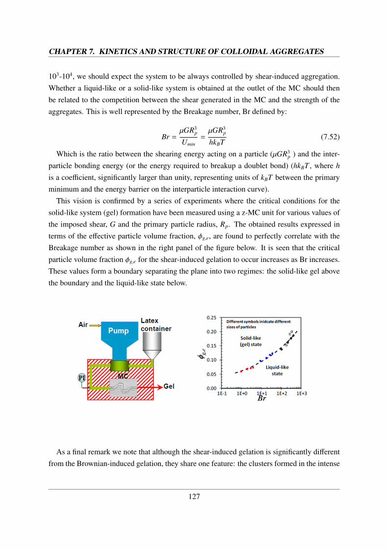
CHAPTER 7. KINETICS AND STRUCTURE OF COLLOIDAL AGGREGATES
103-104, we should expect the system to be always controlled by shear-induced aggregation.Whether a liquid-like or a solid-like system is obtained at the outlet of the MC should thenbe related to the competition between the shear generated in the MC and the strength of theaggregates. This is well represented by the Breakage number, Br defined by:
Br =µGR3
p
Umin=µGR3
p
hkBT(7.52)
Which is the ratio between the shearing energy acting on a particle (µGR3p ) and the inter-
particle bonding energy (or the energy required to breakup a doublet bond) (hkBT , where h
is a coefficient, significantly larger than unity, representing units of kBT between the primaryminimum and the energy barrier on the interparticle interaction curve).
This vision is confirmed by a series of experiments where the critical conditions for thesolid-like system (gel) formation have been measured using a z-MC unit for various values ofthe imposed shear, G and the primary particle radius, Rp. The obtained results expressed interms of the effective particle volume fraction, φg,e, are found to perfectly correlate with theBreakage number as shown in the right panel of the figure below. It is seen that the criticalparticle volume fraction φg,e for the shear-induced gelation to occur increases as Br increases.These values form a boundary separating the plane into two regimes: the solid-like gel abovethe boundary and the liquid-like state below.
As a final remark we note that although the shear-induced gelation is significantly differentfrom the Brownian-induced gelation, they share one feature: the clusters formed in the intense
127
CHAPTER 7. KINETICS AND STRUCTURE OF COLLOIDAL AGGREGATES
shear flow within the MC exhibit fractal scaling with fractal dimension equal to 2.4 ± 0.04,independent of Br, (i.e., of the shear stress, the particle size and the interparticle bondingenergy). This is similar to the case of the Brownian-induced aggregations under DLCA andRLCA conditions, which lead to clusters with fractal dimension equal to 1.8 ± 0.05 and 2.1 ±0.05, respectively, independent of the particle type and size and the electrolyte concentration.
7.7 Experimental Characterization of ColloidalSuspensions
7.7.1 Light Scattering
Scattering of light, x-rays, and neutrons is probably the most important experimental tech-nique used in the investigation of colloidal systems and aggregation phenomena, because itallows one to gain information about the size of particles and aggregates, the structure of ag-gregates and gels, and the kinetics of the aggregation process, in a non-invasive way. Of courseseveral other experimental tools have also been used in the investigation of colloidal systems:microscopy (optical, electron, and X-ray) to study size and morphology; rheology to followthe gel formation and to investigate the mechanical properties of the gel phase; ultrasoundspectroscopy to monitor particle size in on-line applications. In this chapter we will focus ourdiscussion on light scattering, but most of the results could be almost immediately be appliedto both neutrons and x-ray scattering.
In order to better understand the features of light scattering, it is necessary to have anoverview of the physical principles and the main results of scattering theory.
Among the three sources: light, neutron and x-rays, light is the most used one for scatteringexperiments, due to the relatively low cost of lasers which are good quality monochromaticlight sources and due to the development in detectors (photomultipliers and fiber optics) andcomputer-controlled correlators. Another advantage is that light scattering enables one toperform two different kinds of measurements: dynamic light-scattering measurements andstatic light scattering measurements. In the following, we will briefly review the main conceptsof both kinds of measurements. It should be pointed out that most of the static light scatteringtheory can be also applied to neutron and x-rays scattering experiments.
Light scattering is due to the interactions of electromagnetic waves with matter. When anincident electromagnetic wave shines on a molecule, the electrons feel the interaction and, asa results, the center of mass of the negative charges in the molecule is shifted from its original
128
CHAPTER 7. KINETICS AND STRUCTURE OF COLLOIDAL AGGREGATES
position. Then, a dipole is formed, which oscillates with the same frequency as the incidentradiation. One of the major results of the electromagnetic theory is that an oscillating dipoleemits electromagnetic radiation in all directions. This radiation is the scattered radiation.When a sample is illuminated by an incident electromagnetic wave, the sum of the radiationsscattered by all the elements of the sample constitute the scattered radiation. The intensity ofthe scattered light depends strongly on the optical contrast of the scattering object, which isthe difference in refractive index between the object and the surrounding medium.
Another way of understanding the scattering problem is the quantum mechanics perspective,where the incident radiation can be viewed as made of photons traveling in a given direction,and due to the collisions with atoms of the sample, these photons are deviated, or scattered,keeping however their frequency constant. According to this picture, multiple scattering cor-responds to the situation where photons are scattered more than once. Multiple scattering islikely to occur in system with a high concentration of material or in systems with a high opticalcontrast, when the probability of a photon to be scattered more than once is very high.
The general treatment of light scattering is quite complex, especially for the most generalcase where multiple scattering is considered. It requires the full solution of Maxwell equations,which is feasible only for very simple geometries like spheres, cylinders, ellipsoids etc. Thisarises because the multiple scattering problem is a typical many-body problem: the scatteringbehavior of one part of the sample has an effect on, and is affected by, all the other parts of thesample. For complex, but always small, systems, where no analytical solutions of Maxwellequations is available, only heavy numerical methods can be used.
Therefore, for most of the applications in the colloidal domain, the interpretation of scat-tering data is unfortunately limited to those conditions where multiple scattering is absent orcan be safely neglected. From an experimental point of view, the conditions where multiplescattering can be neglected are those of low concentration and low optical contrast, where thenumber of incident photons scattered is a small fraction of the total. An alternative to loweringthe concentration of scatterers is the so-called refractive index matching, i.e., finding a solventthat matches as much as possible the refractive index of the scatterer, so that a very low opticalcontrast can be obtained.
7.7.2 Static Light Scattering
The theory of scattering that neglects multiple scattering is called Rayleigh-Debye-Gans (RDG)theory. The basic assumption is that in every part of the sample, the radiation that illuminates
129
CHAPTER 7. KINETICS AND STRUCTURE OF COLLOIDAL AGGREGATES
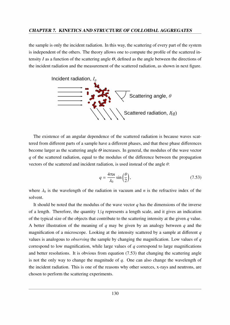
the sample is only the incident radiation. In this way, the scattering of every part of the systemis independent of the others. The theory allows one to compute the profile of the scattered in-tensity I as a function of the scattering angle Θ, defined as the angle between the directions ofthe incident radiation and the measurement of the scattered radiation, as shown in next figure.
Incident radiation, I0
Scattered radiation, I(q)
Scattering angle, θ
The existence of an angular dependence of the scattered radiation is because waves scat-tered from different parts of a sample have a different phases, and that these phase differencesbecome larger as the scattering angle Θ increases. In general, the modulus of the wave vectorq of the scattered radiation, equal to the modulus of the difference between the propagationvectors of the scattered and incident radiation, is used instead of the angle θ:
q =4πnλ0
sin(θ
2
), (7.53)
where λ0 is the wavelength of the radiation in vacuum and n is the refractive index of thesolvent.
It should be noted that the modulus of the wave vector q has the dimensions of the inverseof a length. Therefore, the quantity 1/q represents a length scale, and it gives an indicationof the typical size of the objects that contribute to the scattering intensity at the given q value.A better illustration of the meaning of q may be given by an analogy between q and themagnification of a microscope. Looking at the intensity scattered by a sample at different q
values is analogous to observing the sample by changing the magnification. Low values of q
correspond to low magnification, while large values of q correspond to large magnificationsand better resolutions. It is obvious from equation (7.53) that changing the scattering angleis not the only way to change the magnitude of q. One can also change the wavelength ofthe incident radiation. This is one of the reasons why other sources, x-rays and neutrons, arechosen to perform the scattering experiments.
130
CHAPTER 7. KINETICS AND STRUCTURE OF COLLOIDAL AGGREGATES
X-rays are probably the first source that has been used in the investigation of the structure ofmaterials, particularly crystals. They have been chosen because of their very low wavelengththat results in a high resolution. They are usually applied to investigate gels and surfactantsolutions. X-rays scattering, particularly small angle x-rays scattering, allows to investigatesystems over a broad range of length-scales.
Neutron scattering is based on the scattering of neutrons on the nuclei of atoms. Sinceneutrons can have a high momentum, which is inversely proportional to their wavelength,neutron scattering also provides a very high resolution. Another advantage is that in the casewhere the system under investigation is an aqueous solution, the appropriate mixing of waterand heavy water (D2O) enables the elimination of multiple scattering or to change the contrastin such a way that only some part of a sample can be studied. This method is called contrastvariation technique.
Static light scattering measurements are to determine the profile of the scattered intensity asa function of the modulus of the wave vector q. To be more quantitative, we consider a samplemade of N subunits, having all the same optical properties. In this case, the intensity of thescattered radiation is given by:
I(q) =I0
r2
N∑j=1
N∑m=1
b j(q)b∗m(q) exp(−i q ·
(R j − Rm
)), (7.54)
where I0 is the intensity of the incident radiation, r is the distance of the sample from thedetector (assumed to be much larger than the size of the sample), R j is the vector defining theposition of the center of the jth subunit with volume V j, i is the imaginary unit, the asteriskdefines the complex conjugate, and the quantity b j(q), called scattering length, is defined asfollows:
b j(q) =πn2
λ20
n2p − n2
n20
∫V j
exp(−i q · r j
)d3r j, (7.55)
where np is refractive index of the material, n0 is the average refractive index of the dispersion(material and dispersant) and r j is the vector defining the coordinate of a point inside thejth subunit at a distance r j from its center of mass. It is important to notice that equation(7.54) is very general, and holds true not only for light scattering but also for neutron andx-rays scattering. The only difference for different radiation sources is the dependence ofthe scattering length on the physical properties responsible for the scattering behavior of thesystem, namely the term multiplying the integral in equation (7.55).
From equations (7.54) and (7.55) three very important features of intensity of scatteredlight can be recognized. First of all, the scattered intensity is proportional to the reverse
131
CHAPTER 7. KINETICS AND STRUCTURE OF COLLOIDAL AGGREGATES
fourth power of the wavelength. This explains among others why the sky appears blue: thecomponent of white sun’s light which is diffused more heavily by dust particles and waterdroplets is blue light (low wavelength). The second important feature is that the intensity ofscattered light is proportional to the square of the volume of the object. Therefore, in thepresence of a population of large and small particles, the amount of light scattered by largeparticles easily overwhelms that of small particles. The third feature is that the intensity ofscattered light strongly depends on the optical contrast between the material and the mediumaround it. If the optical contrast is reduced to zero, the intensity of scattered light also goes tozero.
Since equation (7.54) is quite complex, requiring the knowledge of the relative distancesamong the various subunits in the sample, it is useful to consider a special case of equation(7.54) that is very important for all colloidal applications. In particular, let us assume that allthe subunits are equal and of spherical shape, then equation (7.54) takes the form:
I(q) = I0K1NV2p P(q)S (q), (7.56)
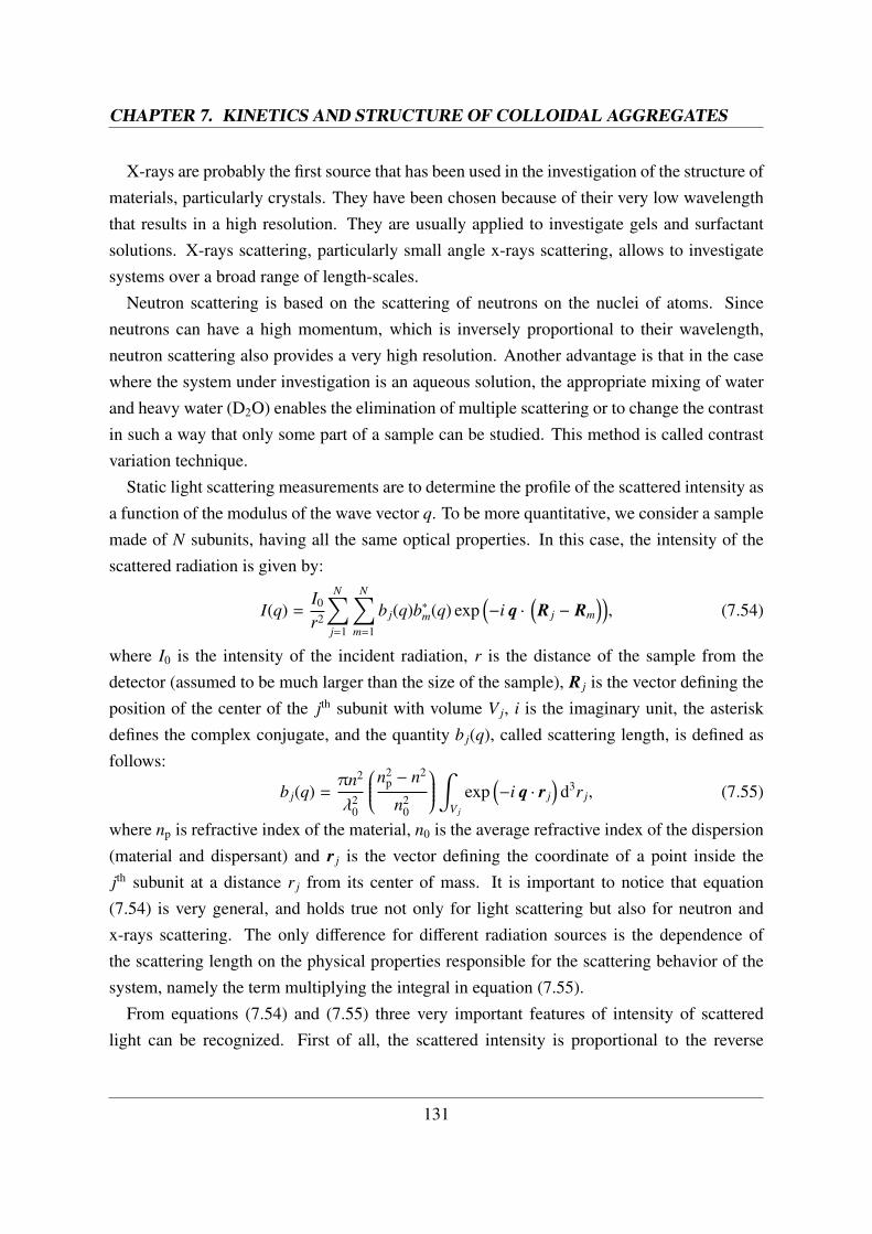
where Vp is the volume of one spherical particle, K1 is a constant that incorporates the de-pendence of equation (7.54) on the optical constants, P(q) is called particle form factor anddepends on the geometrical shape and size of a particle, and S (q) is the structure factor, whichdepends on the correlations among the particles. In the case of spherical particles, the formfactor P(q) is given by:
P(q) =
[3(sin(qRp) − qRp cos(qRp))
(qRp)3
]2
, (7.57)
The form factor for a sphere is plotted in the next figure.
This formula is correct usually for particles sufficiently smaller than the wavelength of theradiation (about 10 times smaller), and with a low optical contrast. If the particles do notfulfill these requirements, the RGD theory cannot be applied to interpret the scattering profileof particles. Instead, the full scattering theory, referred to as Mie theory, has to be used.
From a Taylor expansion of the particle form factor, one can derive a very useful relation:
P(q) = 1 −13
q2R2g,p, (7.58)
where Rg,p is the primary particle radius of gyration. Equation (7.58) suggests that, from thebending of the form factor, one can estimate the radius of gyration of an object. The radius of
132
CHAPTER 7. KINETICS AND STRUCTURE OF COLLOIDAL AGGREGATES
gyration of an object is defined as the sum of the squares of the distances of all his points fromthe center of mass:
R2g,p =
1i
i∑j=1
(r j − rcm
)2, (7.59)
For a continuous object, the sum in the above equation should be replaced by an integral. Inthe case of a sphere, Rg,p =
√3/5Rp.
The structure factor, S (q), on the other hand, contains information about the structure ofthe system, i.e., how the particles are arranged. The relation between the structure factor andrelative positions of i spherical particles in the system is given by the following expression:
S (q) =1i2
i∑m, j=1
sin(qrm j)qrm j
, (7.60)
where rm j is the distance between the centers of the mth and the jth particles. If the system isdilute enough that no correlations among the particles exist, i.e., the relative distances amongthe particles are much larger than 1/q, then S (q) = 1 and the scattering intensity depends onlyon the geometrical properties of the particles.
The general procedure to obtain the structure factor of a system from static scattering mea-surements is as follows. One first determines the particle form factor P(q) by performingthe static scattering measurements for a dilute suspension of particles, where S (q) = 1 andthe measured profile is only proportional to the form factor. Then, by dividing the scatteringprofile of the sample by the obtained form factor, the structure factor can be analyzed.
Two kinds of information from the structure factor are crucial in the study of aggregationphenomena. In the case of a dilute suspension of large fractal aggregates, it can be shown that
133
CHAPTER 7. KINETICS AND STRUCTURE OF COLLOIDAL AGGREGATES
the structure factor has typically a power-law behavior within a certain q-range:
S (q) ∼ q−df , (7.61)
so that from the slope of S (q) in a double logarithmic plane the cluster fractal dimension df
can be extracted. The validity of this procedure will be subsequently discussed in the case ofsmall clusters and in the case of gels. Another important quantity that can be determined fromthe scattering profile is the radius of gyration. It can be obtained by using a Taylor expansionsimilar to what was done for a single particle. This procedure is called Zimm plot analysis:
P(q)S (q) = 1 −13
q2R2g, (7.62)
where a linear region can be found when plotting P(q)S (q) versus q2, the slope of which isproportional to the square of the radius of gyration of the system.
All the theory summarized above refers to a system in which there is no polydispersity.When a polydisperse system is analyzed, the effect of the polydispersity on the scattered in-tensity has to be taken into account. It can be seen from equation (7.56) that, since the intensityscattered by each particle is proportional to the square of its volume (proportional to the squareof the mass), large particles contribute much more to the total scattered intensity than smallparticles. In particular, in the case of a dilute population of particles with m different classesof particles, the total scattered intensity becomes:
I(q) = I0K1
m∑j=1
NiV2p, jP j(q), (7.63)
where N j, Vp, j and P j(q) are respectively the number, volume and form factor of the jth classparticles. Moreover, even for a monodisperse colloidal system, when the aggregation of theprimary particles occurs, since the population of aggregates is often broad, the expression ofthe scattered intensity becomes:
I(q) = I0K1V2p P(q)
imax∑i=1
Nii2S i(q), (7.64)
where Ni and S i(q) are the number and structure factor of a cluster with mass i and imax is thelargest mass of the clusters in the population.
Consistently, the measured radius of gyration will be an average value 〈Rg〉, which, can be
134
CHAPTER 7. KINETICS AND STRUCTURE OF COLLOIDAL AGGREGATES
written in the following form:
〈Rg〉2 =
imax∑i=1
Ni(t)i2R2g,i
imax∑i=1
Ni(t)i2
. (7.65)
Equation (7.65) shows that the average radius of gyration receives a much greater contributionfrom large clusters than from small clusters. This is again a consequence of the dependenceon the square of the volume of the radiation scattered by an object.
7.7.3 Dynamic Light Scattering
The second scattering technique often used in the study of the colloidal systems and aggrega-tion phenomena is dynamic light scattering, which measures, instead of the scattered intensityas a function of the scattering angle, the rapid fluctuations of the intensity at one specific an-gle. In a colloidal suspension, the configuration of the system changes rapidly with time dueto the Brownian motion of the particles, and consequently, so does the pattern of the scatteredradiation. Moreover, such random motion of the particles (or clusters) results that the config-uration of the system at a certain time t loses quickly any correlation with its initial status. Aneffective way to analyze such irregular change in the scattered intensity induced by the ran-dom motion of particles (or clusters) is to compute the intensity time autocorrelation function〈I(q, 0)I(q, τ)〉:
〈I(q, 0)I(q, τ)〉 = limT→∞
1T
∫ T
0I(q, t)I(q, t + τ)dt, (7.66)
where I(q, t) is the scattered intensity at time t and τ is the delay time. When the delay timeτ = 0, the intensity autocorrelation function is equal to the mean square intensity, and it decaysto the square of the average intensity when the delay time τ goes to infinity. For the latter, thesystem has lost any correlation with its initial configuration. The above analysis is possibleonly if the system is fully ergodic, i.e., as time goes by, the system has the freedom to probeall the possible configurations and does not retain memory of previous stages. Dynamic lightscattering can be used to investigate even concentrated colloidal suspension, to recover inter-esting information about the mobility of particles at high volume fractions and in the presenceof multi-body interactions, but through a very complicated and sophisticated analysis. In thisparagraph we will focus our attention only on the case of dilute colloidal suspensions.
135
CHAPTER 7. KINETICS AND STRUCTURE OF COLLOIDAL AGGREGATES
It is useful to introduce the normalized intensity autocorrelation function:
g(2)(τ) =〈I(q, 0)I(q, τ)〉〈I(q)〉2
, (7.67)
where 〈I(q)〉 is the average intensity. It can be shown that g(2)(τ) is related to another autocor-relation function, the electric field autocorrelation function g(1)(τ), defined as:
g(1)(τ) =〈E(q, 0)E∗(q, τ)〉
〈I(q)〉, (7.68)
where E(q, τ) is the electric field of the scattered wave at delay time τ and wave vector q, andE∗(q, τ) is the complex conjugate. The relation between the two autocorrelation functions iscalled Siegert relation:
g(2)(τ) = 1 + σ(g(1)(τ)
)2, (7.69)
where σ is a constant that depends on the specific configuration of the detector used in theexperiment, but it is always smaller than unity and approaches 1 with increasing the detectorarea. It can be shown that in the case of a dilute suspension of equal size, non-interactingspherical particles, the field autocorrelation function decays exponentially, and the time con-stant is proportional to the particle diffusion coefficient Diff:
g(1)(τ) = exp(−Diffq2τ
). (7.70)
From equation (7.70), it can be seen that the faster the particle move, the larger their diffu-sion coefficient and the faster is the decay of the exponential. Therefore, by measuring g(2)(τ),g(1)(τ) can be extracted using the Siegert relation, equation (7.69), and from the slope of thelogarithm of g(1)(τ), one can determine the diffusion coefficient, and consequently the hydro-dynamic radius Rh using the Stokes-Einstein relation:
Diff =kT
6πηRh, (7.71)
For a sphere, the hydrodynamic radius is equal to the sphere radius. For any other body,equation (7.71) defines the hydrodynamic radius as the size of the equivalent sphere that ex-periences the same friction as the body.
In the case of a polydisperse suspension, equation (7.70) does not hold any longer. Thecontribution of particles (clusters) of different sizes to the total field autocorrelation functionis proportional to their masses squared and to their scattering form factors (structure factors).
136
CHAPTER 7. KINETICS AND STRUCTURE OF COLLOIDAL AGGREGATES
In the case of a population of clusters, equation (7.70) becomes:
g(1)(τ) =
imax∑i=1
Nii2S i(q) exp(−Diff,iq2τ
)imax∑i=1
Nii2S i(q)
. (7.72)
It is clear that measurements performed at different angles, i.e., at different q values, givedifferent results. An important consequence of equation (7.72) is that only an average diffusioncoefficient can be estimated, and therefore an average hydrodynamic radius 〈Rh〉:
〈Rh〉 =
imax∑i=1
Ni(t)i2S i(q)
imax∑i=1
Ni(t)i2S i(q)Reff
h,i
, (7.73)
where Reffh,i is an effective hydrodynamic radius of a single cluster with mass i, accounting also
for the rotational diffusive motion of the cluster.
From Eqs. (7.73) and (7.65), it can be seen that dynamic light scattering and static lightscattering alow one to determine two different average sizes of the CMD. These sizes areindependent moments of the CMD, and contain independent information on the width of theCMD, thus useful information for the CMD analysis. These are also the formulas that allowone to relate measurable quantities to the results of PBE computations.
7.8 Zeta Potential, Electrophoretic Mobility, and SurfaceCharge Density
When working with electrostatically stabilized particles, it is particularly important to de-termine their surface charge status. This is typically carried out by using a combination oftechniques.
The first step usually consists in measuring the surface charge density, or to be more precisethe maximum surface charge density. Potentiometric titration can be used for this purpose.Potentiometric titration consists in using either a concentrated base or a concentrated acid,which are added in small quantities, and simultaneously measuring the conductivity of thesuspension. Titration works exactly as in the case of common acids or base solutions. It
137
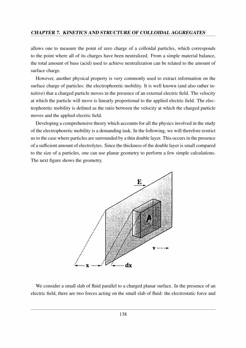
CHAPTER 7. KINETICS AND STRUCTURE OF COLLOIDAL AGGREGATES
allows one to measure the point of zero charge of a colloidal particles, which correspondsto the point where all of its charges have been neutralized. From a simple material balance,the total amount of base (acid) used to achieve neutralization can be related to the amount ofsurface charge.
However, another physical property is very commonly used to extract information on thesurface charge of particles: the electrophoretic mobility. It is well known (and also rather in-tuitive) that a charged particle moves in the presence of an external electric field. The velocityat which the particle will move is linearly proportional to the applied electric field. The elec-trophoretic mobility is defined as the ratio between the velocity at which the charged particlemoves and the applied electric field.
Developing a comprehensive theory which accounts for all the physics involved in the studyof the electrophoretic mobility is a demanding task. In the following, we will therefore restrictus to the case where particles are surrounded by a thin double layer. This occurs in the presenceof a sufficient amount of electrolytes. Since the thickness of the double layer is small comparedto the size of a particles, one can use planar geometry to perform a few simple calculations.The next figure shows the geometry.
We consider a small slab of fluid parallel to a charged planar surface. In the presence of anelectric field, there are two forces acting on the small slab of fluid: the electrostatic force and
138
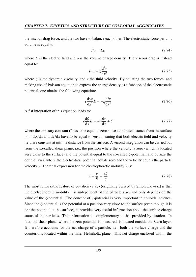
CHAPTER 7. KINETICS AND STRUCTURE OF COLLOIDAL AGGREGATES
the viscous drag force, and the two have to balance each other. The electrostatic force per unitvolume is equal to:
Fel = Eρ (7.74)
where E is the electric field and ρ is the volume charge density. The viscous drag is insteadequal to:
Fvis = ηd2vdx2 (7.75)
where η is the dynamic viscosity, and v the fluid velocity. By equating the two forces, andmaking use of Poisson equation to express the charge density as a function of the electrostaticpotential, one obtains the following equation:
εd2ψ
dx2 E = −ηd2vdx2 (7.76)
A fist integration of this equation leads to:
εdψdx
E = −ηdvdx
+ C (7.77)
where the arbitrary constant C has to be equal to zero since at infinite distance from the surfaceboth dψ/dx and dv/dx have to be equal to zero, meaning that both electric field and velocityfield are constant at infinite distance from the surface. A second integration can be carried outfrom the so-called shear plane, i.e., the position where the velocity is zero (which is locatedvery close to the surface) and the potential equal to the so-called ζ-potential, and outsize thedouble layer, where the electrostatic potential equals zero and the velocity equals the particlevelocity ν. The final expression for the electrophoretic mobility u is:
u =ν
E=εζ
η(7.78)
The most remarkable feature of equation (7.78) (originally derived by Smoluchowski) is thatthe electrophoretic mobility u is independent of the particle size, and only depends on thevalue of the ζ-potential. The concept of ζ-potential is very important in colloidal science.Since the ζ-potential is the potential at a position very close to the surface (even though it isnot the potential at the surface), it provides very useful information about the surface chargestatus of the particles. This information is complementary to that provided by titration. Infact, the shear plane, where the zeta potential is measured, is located outside the Stern layer.It therefore accounts for the net charge of a particle, i.e., both the surface charge and thecounterions located within the inner Helmholtz plane. This net charge enclosed within the
139
CHAPTER 7. KINETICS AND STRUCTURE OF COLLOIDAL AGGREGATES
surface of shear, is smaller than the charge estimated from titration measurements, but moreuseful in studying colloidal stability of particles.
Equation (7.78) is only valid for small double layers compared to the particle size. Wheninstead the double layer is larger than the particle size, Debye proved that the electrophoreticmobility is equal to 2/3 of the values predicted by equation (7.78). A more complete theory,developed by Henry, provides accurate results for all double layer thicknesses, but only for lowsurface potentials, and shows that the electrophoretic mobility increases monotonically fromthe Debye limit to the Smoluchowski limit. However, a non-monotonic behavior is observedfor high surface potentials, as shown in the next figure. These curves are obtained using morecomplex numerical calculations. In addition, a weak dependence on the type of electrolytepresent in the system has been also observed.
Nowadays electrophoretic mobility is most often measured through a combination of DLSand electrophoresis. In fact, in the presence of an electric field, the field autocorrelation func-tion of a particle takes the following form:
g(1)(τ) = exp (±iqEuτ) exp(−Diffq2τ
). (7.79)
where i is the imaginary unit. Therefore, the autocorrelation function shows a typical oscil-lating pattern in the presence of an electric field, the frequency of which equals qEu. The
140
CHAPTER 7. KINETICS AND STRUCTURE OF COLLOIDAL AGGREGATES
electrophoretic mobility can then be obtained by fitting the frequency of these oscillations,and from this the particles zeta potential is calculated.
141