Chapter 8

Hypothesis Testing I

Significant Differences Hypothesis testing is designed to detect

significant differences: differences that did not occur by random chance.

This chapter focuses on the “one sample” case: we compare a random sample against a population.

We compare a sample statistic to a population parameter to see if there is a significant difference.

Example The education department at a large state

university has been accused of “grade inflation” such that education majors have higher GPAs than students in general.

GPAs of all education majors should be compared with the GPAs of all students. There are 1000s of education majors, far too

many to interview. How can the dispute be investigated without

interviewing all education majors?

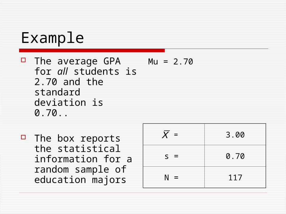
Example The average GPA

for all students is 2.70 and the standard deviation is 0.70..

The box reports the statistical information for a random sample of education majors

Mu = 2.70

X

= 3.00

s = 0.70

N = 117

Example There is a difference between the

parameter (2.70) and the statistic (3.00). It seems that education majors do have higher

GPAs, at least in our sample. However, we are working with a random

sample (not all education majors). The observed difference may have been

caused by random chance.

Two Explanations for the Difference

1. The mean for all education students is the same as the pop. mean (2.70).

The difference in the sample mean is caused by random chance.

2. The difference is real (significant). Education majors have higher GPAs than

students in general

Hypotheses

1. Null Hypothesis (H0) “The difference is caused by random chance”.

The H0 always states there is “no significant

difference.”

2. Alternative hypothesis (H1) The mean GPA for all education majors is higher than

the mean GPA for all students in the college. (H1) always contradicts the H0.

If we can reject the null hypothesis, our data support the alternative hypothesis (but don’t prove it)

Testing the two explanations

Assume that H0 is true. What is the probability of getting the

sample mean (3.0) if the H0 is true and

all education majors really have a mean of 2.7?

If the probability is less than 0.05, reject the null hypothesis.

Test the Hypotheses This will be a one-tailed test since our alternative

hypothesis is not just that education majors’ GPAs are different but that they are higher.

At a 95% confidence level, we put the whole .05 in the upper tail of the normal sampling distribution.

Using the Z score formula and Appendix A to determine the probability of getting the observed difference, we find that Z(critical) = +1.65.

If Z(obtained) is at or above 1.65, we can reject the null hypothesis. The zone of rejection begins at 1.65 and includes any z-score higher than that

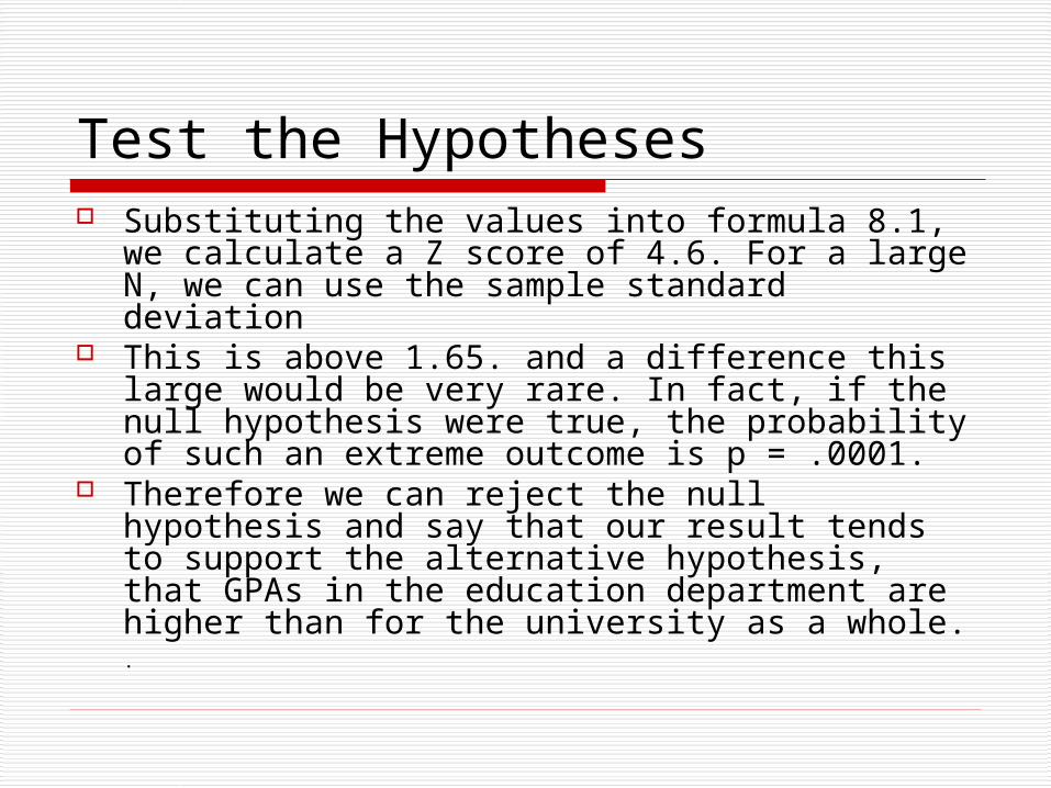
Test the Hypotheses Substituting the values into formula 8.1, we

calculate a Z score of 4.6. For a large N, we can use the sample standard deviation

This is above 1.65. and a difference this large would be very rare. In fact, if the null hypothesis were true, the probability of such an extreme outcome is p = .0001.

Therefore we can reject the null hypothesis and say that our result tends to support the alternative hypothesis, that GPAs in the education department are higher than for the university as a whole. .

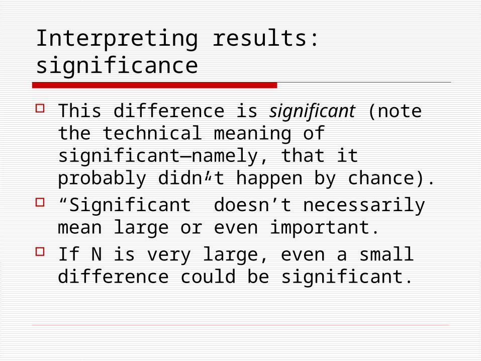
Interpreting results: significance

This difference is significant (note the technical meaning of significant—namely, that it probably didn’t happen by chance).

“Significant” doesn’t necessarily mean large or even important.

If N is very large, even a small difference could be significant.

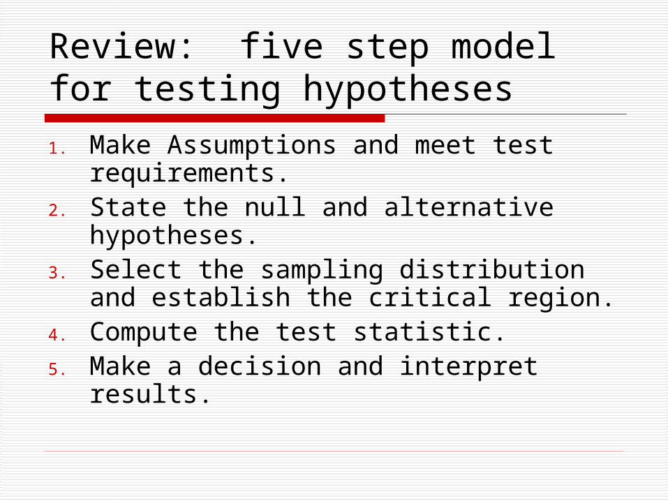
Review: five step model for testing hypotheses

1. Make Assumptions and meet test requirements.

2. State the null and alternative hypotheses.

3. Select the sampling distribution and establish the critical region.

4. Compute the test statistic.5. Make a decision and interpret results.

The Five Step Model: Do the steps more formally

Is there a grade inflation problem in the education dept?

Step 1 Make Assumptions and Meet Test Requirements Random sampling

Hypothesis testing assumes samples were selected according to EPSEM.

The sample of 117 was randomly selected from all education majors.

LOM is Interval-Ratio GPA is I-R so the mean is an appropriate

statistic. Sampling Distribution is normal in shape

This is a “large” sample (N>100).

Step 2 State the Null Hypothesis

Null Hypothesis: μ(education department) = 2.7, the same as the mean for the university as a whole The sample of 117 comes from a

population that has a GPA of 2.7. The difference between 2.7 and 3.0 is

trivial and caused by random chance.

Step 2 State the Alternative Hypothesis

Alternative (or research) hypothesis: Mean in education is higher than 2.7 The sample of 117 probably comes from

a population that has a higher GPA than 2.7.

The difference between 2.7 and 3.0 probably reflects an actual difference between education majors and other students.

Step 3 Select Sampling Distribution and Establish the Critical Region

Sampling Distribution= Z Alpha (α) = .05 Any difference with a probability less than α

is rare and will cause us to reject the H0. Critical Region begins at +1.65

This is the critical Z score associated withα = .05, eon-tailed test.

If the obtained Z score falls in the C.R., reject the H0.

Step 4 Compute the test statistic

Using formula 8.1, Z (obtained) = 4.6

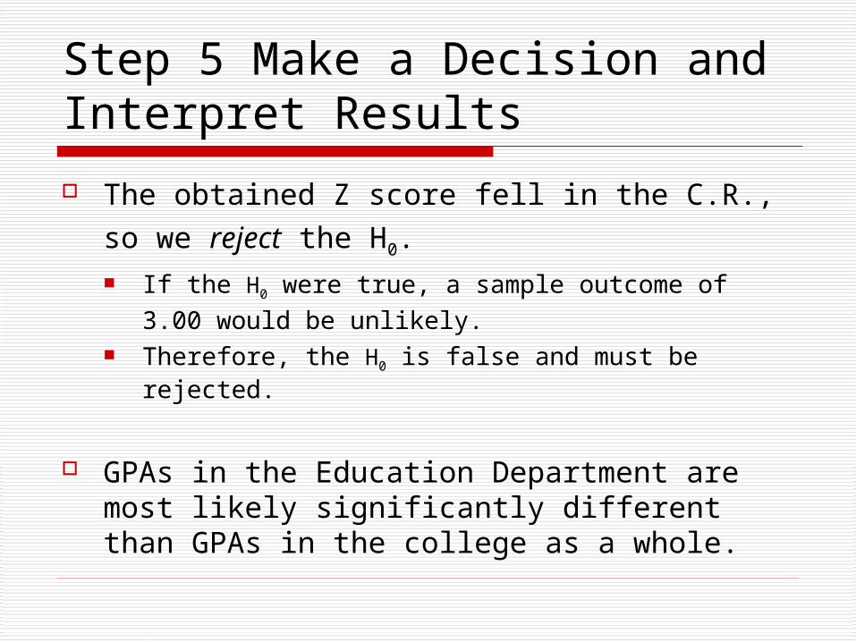
Step 5 Make a Decision and Interpret Results

The obtained Z score fell in the C.R., so we

reject the H0. If the H0 were true, a sample outcome of 3.00

would be unlikely. Therefore, the H0 is false and must be rejected.

GPAs in the Education Department are most likely significantly different than GPAs in the college as a whole.

The Five Step Model: Summary In hypothesis testing, we try to identify

statistically significant differences that did not occur by random chance.

In this example, the difference between the parameter 2.70 and the statistic 3.00 was large and unlikely (p < .05) to have occurred by random chance.

The Five Step Model: Summary

We rejected the H0 and concluded

that the difference was significant. It is very likely that Education majors

have GPAs higher than the general student body

One-tailed vs. two-tailed hypothesis testing

What if our alternative hypothesis were not that education majors have higher GPAs but simply that their GPAs are significantly different than for the student body as a whole

In that case, we do a two-tailed test, and we split the alpha=.05 into both tails (.025 in each)

In that case, z(crit) = +/- 1.96 We’d still use formula 8.1 to calculate

Z(obt)

One-tailed vs. two-tailed hypothesis testing

What if our null hypothesis were that education majors had lower mean GPAs than the student body as a whole.

In that case, the whole alpha (.05) goes into the negative tail of the distribution.

Z(crit) = -1.65 We’d still use formula 8.1 to calculate

z(obt)

Student’s t distribution What if N is smaller than 100? Is there still a

way to test for significance Yes, the student’s t distribution does the

trick. What’s more, as N gets to 100 or more, the

t-distribution behaves just like the Z-distribution, so we can actually just use the t-distribution all the time

What if we had a smaller sample of education majors?

N = 65 Sample mean = 2.9 Sample standard deviation = 0.4

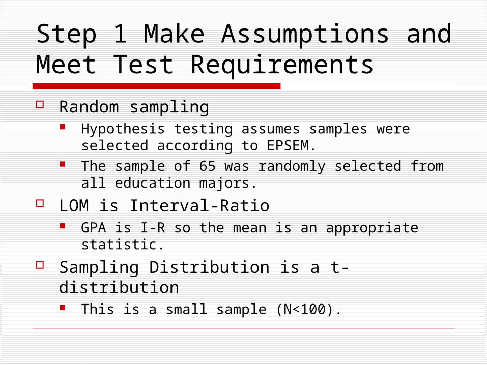
Step 1 Make Assumptions and Meet Test Requirements Random sampling

Hypothesis testing assumes samples were selected according to EPSEM.

The sample of 65 was randomly selected from all education majors.

LOM is Interval-Ratio GPA is I-R so the mean is an appropriate

statistic. Sampling Distribution is a t-distribution

This is a small sample (N<100).

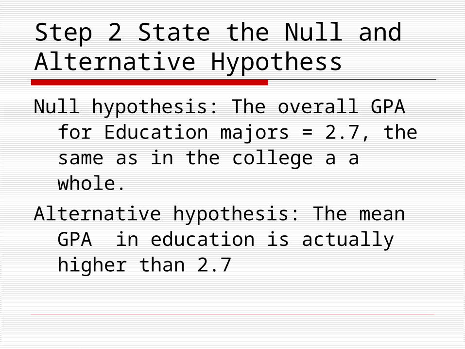
Step 2 State the Null and Alternative Hypothess

Null hypothesis: The overall GPA for Education majors = 2.7, the same as in the college a a whole.

Alternative hypothesis: The mean GPA in education is actually higher than 2.7

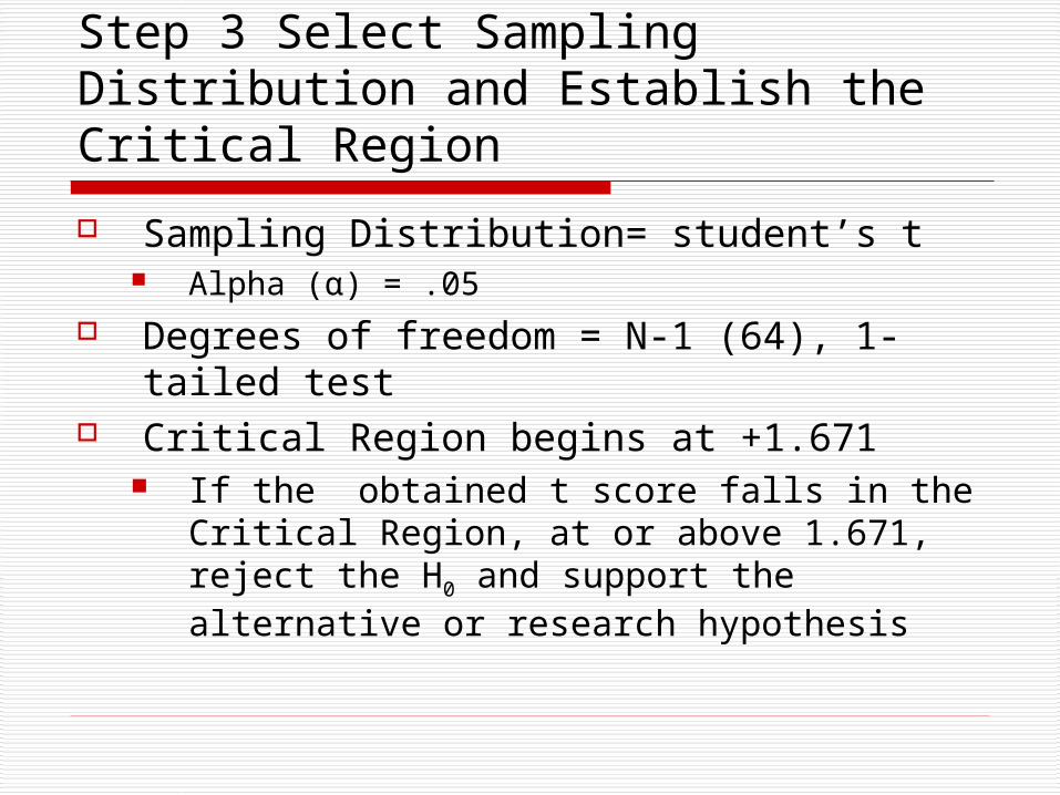
Step 3 Select Sampling Distribution and Establish the Critical Region

Sampling Distribution= student’s t Alpha (α) = .05

Degrees of freedom = N-1 (64), 1-tailed test

Critical Region begins at +1.671 If the obtained t score falls in the Critical

Region, at or above 1.671, reject the H0 and support the alternative or research hypothesis

Step 4 Compute the test statistic

Using formula 8.2, t (obtained) = 4.

Step 5 Make a Decision and Interpret Results

The obtained t score fell in the Critical

Region, so we reject the H0. If the H0 were true, a sample outcome of t = 4

would be unlikely. Therefore, the H0 must be rejected.

Our supports the proposition that education majors have a GPA that is significantly significantly higher than the GPA of the general student body

2 types of error Type 1 or alpha error: the probability of

rejecting the null hypothesis when it is actually true. We set up the problem in a way that minimizes (but does not eliminate) this possibility.

Type 2 or beta error: the probability of failing to reject a null hypothesis when it is actually false.

The two types of error are inversely related; lowering the risk of type 1 error raises the risk of type 2 error