chapter cl finite-difference model for 0 … · techniques of water-resources investigations of the...

Techniques of Water-Resources Investigations of the United States Geological Survey

Chapter Cl

FINITE-DIFFERENCE MODEL FOR 0 AQUIFER SIMULATION IN

TWO DIMENSIONS WITH RESULTS OF

NUMERICAL EXPERIMENTS

By P. C. Trescott, G. F. Pinder, and S. P. Larson

Book 7

AUTOMATED DATA PROCESSING AND COMPUTATIONS

http://www.usgs.gov

reidell

Click here to return to USGS Publications

../index.html

UNITED STATES DEPARTMENT OF TWE INTERIOR

CECIL D. ANDRUS, Secretary

GEOLOGICAL SUR\IEY

H. VVilliam Menard, Director

First printing 1976

Second printing 1980

Requests, at cost, for the Card Deck listed in Attachment VII should be directed to: Ralph N. Either, Chief, Office of Teleprocessing, M.S. 805, National Center,

U.S. Geological Survey, Reston, Virginia 22092.

UNITED STATES GOVERNMENT PRINTING OFFICE, WASHINGTON : 1976

For sale by the Branch of Distribution, U.S. Geological Survey, 1200 South Eads Street, Arlington, VA 22202

PREFACE

The series of manuals on techniques describes procedures for plan- ning and executing specialized work in water-resources investigations. The material is grouped under major headings called books and further sub- divided into sections and chapters; section C of Book ‘7 is on computer programs.

“Finite-difference model for aquifer simulation in two dimensions with results of numerical experiments” supersedes the report published in 1970 entitled, “A digital model for aquifer evaluation” by G. F. Pinder as Chapter Cl of Book 7. The new Chapter Cl represents a significant im- provement in the computational capability to solve the flow equations and has greater flexibility in the hydrologic situations that can be simulated.

III

l

CONTENTS

Abstract _________________________________ Introduction ______________________________ Theoretical development ____________-______

Ground-water flow equation ____________ Finite-difference approximations __---__- Source term __________________________

Leakage __________________________ Evapotranspiration ____ ____________

Computation of head at the radius of a pumping well ______________________

Combined artesian-water-table simulation- Transmissivity ------------------- Storage __________________________ Leakage _________________________

Test problems _____________-______________ Numerical solution ________________________

Line successive overrelaxation __________ Two-dimensional correction to LSOR LSOR acceleration parameter ______

Alternating-direction implicit procedure _____________________________

Strongly implicit procedure ____________ Comparison of numerical results ____________ Considerations in designing an aquifer

model __________________________________ Boundary conditions __________________ Initial conditions _____________________ Designing the finite-difference grid _____

Selected references ________________________ Attachment I, notation ____________________ Attachment II, computer program __________

Main program ________________________

Page 1

1 2 2 2 4 4 7

8 10 11 11 11 12 14 15 17 18

19 21 27

29 29 30 30 32 37 38 38

Attachment II, computer program-Continued Subroutine DATA1 ___-_-_-~-~---~~~--~

Time parameters _----------------- Initialization _____________________

Subroutine STEP ____________-________ Maximum head change for each

iteration _______________________ Subroutine SOLVE ___________________

SIP iteration parameters _-_-__---- Exceeding permitted iterations _____

Subroutine COEF ____________________ Transient leakage coefficients ---_-- Transmissivity as a function of

head __________________________ TR and TC coefficients __-_--__--_-

Subroutine CHECK1 __________________ Subroutine PRNTAI __________________ BLOCK DATA routine ____--------~--- Technical Information ___-__----_~---~

Storage requirements ____________-- Computation time ______--__-----_- Use of disk facilities for storage of

array data and interim results __ Graphical display package _------------ Modification of program logic _-----__-- Fortran IV __________________________ Limitations of program ___--__--__-_--

Attachment III, data deck instructions------ Attachment IV, sample aquifer simulation

and job control language ---_------------ Attachment V, generalized flow chart for

aquifer simulation model _____________-__ Attachment VI, definition of program variables Attachment VII, program listing __-__-__-__

FIGURES

1. Index scheme for Anitedifference grid and coefficients of finite-difference equation written for node (i,i) ________________________________________-----------------------------------

2. In the first pumping period, (a) illustrates the head distribution in the confining bed at one time when transient leakage effects are significant; (b) illustrates a time after transient effects have dissipated; in the second pumping period, (c) is analogous to (a) and (d) is analogous to (b) __________________-_____________________------------------------------------------

3. The total drawdown at the elapsed time, t, in the pumping period (a) is applied at t/3 in equations 9 and 10 to approximate qoc,,,r, the transient part of q’,,,,r (b) _- ___________________ -_

Page

38 38 40 40

40 40 41 41 41 41

41 41 42 42 43 43 43 43

44 46 46 46 48 49

66

68 74 78

Page

2

6

6

V

VI I CONTENTS

4.

6.

6.

7. 8.

9. 10. 11.

12. 13. 14.

16.

16.

17. 18. 19.

20. 21. 22. 23. 24. 25. 26. 27. 28.

29. 30.

31.

32. 33.

Comparison of analytic solution and numerical results using factors of 2 and 3 in the transient leakage approximation ________________________________________------------------------

Percent difference between the volume of leakage computed with the model approximation and Hantush’s analytical results _________________------.-------------------------------------

Evapotranspiration decreases linearly from &., where the water table is at land surface to zero where the water table is less than or equal to Gc,&X~ --_---____________________________

Flow from cell (i’l,i) to cell (ii) (a) and equivalent rad*ial flow to well (i,i) with radius rs (b) __ Storage adjustmen i- is applied to distance A in conversion from artesian to water-table conditions

(a) and to distance B in conversbon from water-table to artesian conditions (b) _____-__-__ Two of the possible situations in which leakage is restricted in artesian-water-table simulations _- Characteristics of test problem 1 _________ - _____________ -----_--__--__-- ______________ --___- Transmissivity and observed water-ta.ble configuration for teet problem 2 (fieldwork and model

design by Konikow, 1976) ________________________________________---------------------- Characteristics of test problem 3 ____________________ - __.________ --_--_-- ____________________ Hypothetical problem with 9 interior nodes -- ____ - ____ -_-----_--___- ____________________---- Number of iterations required for solution by LSOR and LSOR + 2DC using different accelera-

tion parameters __________-_-----_-----~~~~~-~----~.~~~~--~~-----~--~~~~~~~~~~~~~~~~~~~~ Reduction in the maximum residual for problems 1 to 3 for selected ~,a,, used to compute the

AD1 parameters ______-_--__---_-_----~~~~~-~-~~~~~~~~~-~~--~~~~--~~~~~~~~~~~~~~~~~~~~ Number of iterations required for solution of the test problems with AD1 using different num-

bers of parameters --_-____________--______________________--------------------------- Coefficients of unknowns in equation 27 ________________________________________-------------- Reverse numbering1 scheme for 3 x 3 problem---- ______________ -___--__-- ____________________ Iterations required ‘for solution of the test problem by SIF’ using different numbers and sequences

of parameters ____---_--_____-________________________-------------------------------- Computational work required by different iterative techniques for problem 1 ___- _______________ Computational work requi’red by different iterative techniques for problem 2 ______ - ____________ Computational work required by different iterative techniques for problem 3 ______--____-__--__ Computational work required by different iterative technisques for problem 4 __________________ Number of iterations required for solution of problem 4 by SIP using different values of p’ --_-_ Variable, block-centered grid with mi zed boundary conditions ___- -_ --_ -_ - -_ __ _ __ _____________ Orientation of manon computer page __- _________ ---_- __________ --___-__--_---------________ Additional FORTRAN code required to produce output for graphical displav __-__-_-________ Water level versus time at various n,odes of the sample aquifer problem produced by the graphi-

cal display padkage _______-____---_-__-____________________--------------------------- Contour map of water level for sample aquifer problem produced by graphical display package _ Cross section illustrates several options included in the sample ,problem and identifies the meaning

of several program parameters ___________________-____________________----------------- JCL and data deck ‘to copy some of the data sets on disk, compute for 5 iterations, and store the re

sults on disk -_-__-__________________________________---------------------------------- JCL and data deck tto continue the previous run (fig. 31) te a solution -- ____ - _____ - _____________ JCL and data deck’ to simulate the sample problem without using disk files _______ - ___________

TABLES

1. Comparison of drawdowns computed with equation 16 and the analytic values _________________ 2. Number of arrays required for the options ____________________ --___-__--___- _____ -__--- _____

Page 0

7

8

9 9

11 12 13

14 15 16

19

22

23 24 25

26 27 28 28 28 28 31

0

43 47

48 49

65

66 57 68

Page 10 38

3. Arrays passed to the subroutines and their relative location in the vector Y ------------------- 39

FINITE-DIFFERENCE MODEL FOR AQUIFER SIMULATION IN TWO DIMENSIONS WITH RESULTS OF

NUMERICAL EXPERIMENTS

By P. C. Trescott, G. F. Pinder, and S. P. Larson

Abstract The model will simulate ground-water flow in an

artesian aquifer, a water-table aquifer, or a combined artesian and water-table aquifer. The aquifer may be heterogen,eous and anisotropic and have irregular boundaries. The source term in the flow equation may include well discharge, constant recharge, leakage from confining beds in which the effects of storage are considered, and wapotranspiration as a linear function of depth to watex.

The theoretical development includes presentation

0

of the appropriate flow equations and derivation of the finite-difference approximations (written for a variable grid). The documentation emphasizes the numerical techniques that can be used for solving the simultaneous equations and describes the results of numerical experiments using these techniques. Of the three numerical techniques available in the model, the strongly implicit procedure, in general, requires less computer time and has fewer numerical difficulties than do the iterative alternating direction implicit procedure and line successive overrclaxation (which includes a two-dimensional correction procedure to accelerate convergence).

The documentation includes a flow chart, program listing, an example simulation, and sections on designing an aquifer model and requirements for data input. It illustrates how model results can be presented on the line printer and pen plotters with a program that utilizes the graphical display software available from the Geological Survey Computer Center Division. In addition the model includes options for reading input data from a disk and writing intermediate results on a disk.

Introduction The finite-difference aquifer model docu-

mented in this report is designed to simulate in two dimensions the response of an aquifer to an imposed stress. The aquifer may be

artesian, water table, or a combination of artesian and water table ; it may be heterogeneous and anisotropic and have irregular boundaries. The model permits leakage from confining beds in which the effects of storage are considered, constant recharge, evapotranspiration as a linear function of depth to water, and well discharge. Although it was not designed for cross-sectional problems, the model has been used with some success for this type of simulation.

The aquifer simulator has evolved from Pinder’s (1970) original model and modifications by Pinder (1969) and Trescott (1973). The model documented by Trescott (1973) incorporates several features described by Prickett and Lonnquist (1971) and has been applied to a variety of aquifer simulation problems by various users. The model described in this report is basically the same as the 1973 version but includes minor modifications to the logic and data input. In addition, the user may choose an equation solving scheme from among the alternating direction implicit procedure, line successive overrelaxation, and the strongly implicit procedure. The program is arranged so that other techniques for solving simultaneous equations can be coded and substituted for the iterative techniques included with the model.

The documentation is intended to be re;G sonably self contained, but it assumes that the user has an elementary knowledge of the physics of ground-water flow, finite-difference methods of solving partial differential

1

2 T+HNIQUES OF WATER-RESOURCES INVESTIGATIONS

equations, matrix lgebra, and the FOR- TRAN IV language. B

Theoretical Development

Ground-watgr flow equation The partial differential equation of ground-

water flow in a confined aquifer in two dimensions may be written as

in which

W(x, y, t) is the volumetric flux of re-

T,,, T,,, T,,, T&, are the components of

charge or withdrawal per

the transmissivity tensor

unit surface area of the

yt-1) ; h is hydraulic head (L) ;

aquifer (Libl).

S is /the storage coefficient (dimensionless) ;

The reader is referred to Pinder and Brede- hoeft (1968) for development and discussion of equation 1. In the simulation modcel, equation 1 is simplified by assuming that the Cartesian coordinate axes x and y are alined with the principal components of the transmissivity tensor, T,,iand T,,, giving

In water-table aquifers, transmissivity is a function of head. Assuming that the coordinate axes are co-linear with the principal components of the hydraulic conductivity tensor, the flow equation may be expressed as (Bredehoeft and Pinder, 1970)

in which

K,,, ,K,, are the principal components of the hydraulic conductivity tensor (U-l) ;

s, is the specific yield of the aquifer (dimensionless) ;

h is the saturated thickness of the aquifer (~5).

Finite-difference approximations In order to solve equation 2 or 3 for a

Utilizing a block-centered, finite-difference

heterogeneous aquifer with irregular boun-

grid in which variable grid spacing is per-

daries, one approach is to subdivide the re- gion into rectangular blocks in which the

mitted (fig. 1), equation 2 may be approxi-

aquifer properties are assumed to be uniform. The continuous derivatives in equations 2 and 3 are replaced by finite-difference

mated as

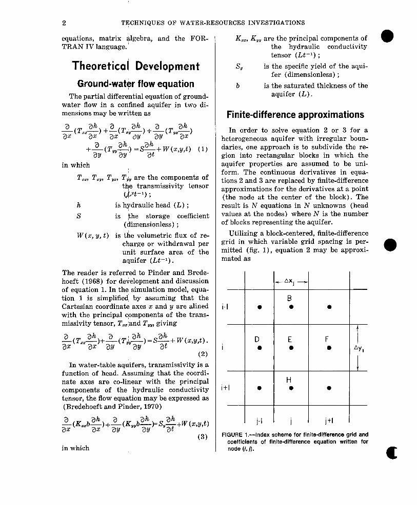
approximations for the derivatives at a point (the node at the center of the block). The result is N equations in N unknowns (head values at the nodes) where N is the number of blocks representing the aquifer.

--

i-l

I

--

i+l

bXJ -I B I

0 a

I D I l

D E F 0 0 0

I I H 0 0 0

j-l I j I jtl

FIGURE l.--Index scheme for finite-difference grid and coefficients of finite-difference equation written for node (i, j).

c

FINITE-DIFFERENCE MODEL FOR AQUIFER SIMULATION 3

+~[(Tu~)i+~,j-~u~)*-,,,3

="s (h,j,k- h,j,k-1) + Wi,j,k (4)

in which

AX] is the space increment in the x direc-

tion for column j as shown in figure 1 (;L);

Ayi is in the space increment in the y direction for row i as shown in figure 1 (G) ;

At is the time increment (t) ; i is the index in the y dimension ; j is the index in the x dimension ; k is the time index.

Equation 4 may be approximated again as

T (kj+l,k-ki.k) I[ _ T (&r- ki-I,k) =o(i,j+%)

AX1+ ?4 IE (i,j-%)

AXi.-% II Tuu (i+%.j) (h+~,j,k--h.j,k) I[ _ T (hij,k--hi-1,j.k)

AYi+. uu +-%A AYi-l/

=g(h,j,k- hi,j,k-1) + wi,j,k

in which

T,, (i,j+j/,) #is the transmissivity between node (i,j) and node (i,j+ 1) ;

Ax i+‘h is the distance between node (i,j) and node (i,j+ 1).

Equation 5 is written implicitly, that is, the head values on the IefLhand side are at the new (k) time level. Following a convention similar to that introduced by Stone (1968), the notation in equation 6 may be simplified by writing

Fi,j(h,j+l,k- h,j,k) -D&j (h,j,k- hi,j--l,k)

+Hi,j(h+l,j,k- k,j,k) -Bi,j (h,j,k-hi-l,j,k)

in which

TV, [t.jl Ayi--1+ Tyy[i-l.jl Ayi 1 (7a) Bi,j=

4% The term in brackets is the harmonic mean of

T ffu Iid Tuu [i-l.il

ay, &hi--~

It represents the ratio TV,+ 5/z,/Ayi-s in equation 5.

l Similarly,

(5)

2Tiom[i.j] Tm [i.j--11

T .m~t,j] AXj-l+ Tmz~i,j-l]AXj 1 Di,i =

AXj ; Ub)

[

2Tm[i,jl Tm [t,j+ll

Tscrnri,jlAX~+1+ Tm [i.j+l]AXj 1 F,j=

AXj ; (7c)

[

2Tuu~i+l.j] Tuu [i.jl

Tuu[i,jl AY4+1 + Tuu[t+l,jlAY,i 1 H4.j =

AY+ . (7d)

Use of the harmonic mean (1) insures con- tinuity across cell boundaries at steady state if a variable grid is used, and (2) makes the appropriate coefficients zero at no-flow boundaries.

Equation 6 is also used to approximate equation 3 by replacing S with Sy and defin- ing the transmissivities in equations 7a through 7d as a function of the head from the preceding iteration. As an example,

Tinci,jJ =K,,~,i,j,bt~~

in which n is the iteration index. The notation may be simplified further by

omitting subscripts not including a “ + 1” or “-1” (except where necessary for clarity) and by following the convention that un- known terms are placed on the left-hand side

4 TlhCHNIQUES OF WATER-RESOURCES INVESTIGATIONS I

of the equations. 4 quation 6 may be rear- ranged and expressed as

Bh-,+Dh,-,+&+Fh,+,+Hhi+l=Q (8) in which I

E=- (B+D+k+H+

Q= -$hx-,+iW.

Souice term The source term I/V(x,y,t) can incl.ude well

discharge, transientlleakage from a confining bed, recharge from ‘precipitation and evapotranspiration. In the model the source term is computed as I

Wj,j,k = Qw Wkl

Axj Ay.i - qre Ii.j.kl - h,k + qet [i,j,k]

in which 12, Ci,j,LJ is the well discharge (Dt-I) ; ‘&[i,j,k] is the recharge flux per Unit area

(;Lt-1) ; il’i,j,k is the flux per unit area from a

confining layer (Lt-I) ; (I,~ [i,i’,,C1 is the evapotranspiration flux

per unit area (Lt-I).

Leakage

Leakage from a confining layer or stream- bed in which storage is considered may be approxim.ated by

Ki'j h )I) ’ + ---$ b,j,o - k,j,o) (9 1

(K: jt/mi,jS,[ij,) is dimensionless time; see Bredehoeft and Pinder (1970) for a discussion Iof leakage versus dimensionless tim’e ;

t is the elapsed time of I the pumping period

(t) *

in which

ki,i,O

L,j,O

1

1 is the hydraulic head in the aquifer at the start of the pumping

I period (&) ; I is the hydraulic head

Kij >

mi,j

ss[i.jl

I on the other side of the confining bed (L) ;

/ is the hydraulic conductivity of the confining bed (L/t) ;

is the thickness of the confining bed (L) ;

, is the specific storage in the confining layer (L-l) ;

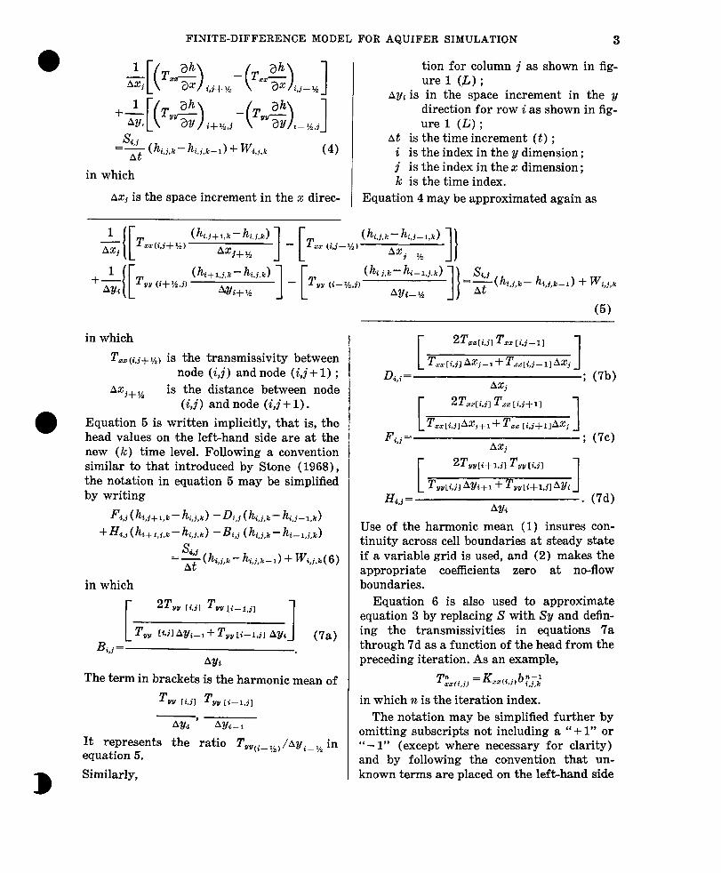
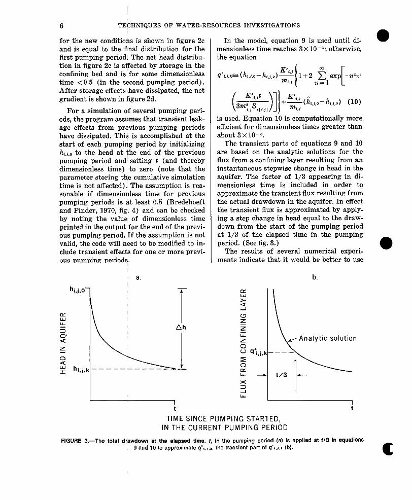
-- Equa.tion 9 is modified from Bredehoeft and Pinder (119’70, p. 887) ; note that it is the sum of two terms ; the first term on the right- 0 hand side of equation 9 considers transient effects ; the second term is steady leakage due to the initial gradient across the confining bed. (See fig. 2.) Figure 2 illustrates the head distribution in the confining layer at any given point in the aquifer system at two different times in each of two successive pumping periods. (The succession of head values in the aquifer is shown by ht,j,l, . . . hi,j,4.) The solid line represents the head distribution at the beginning of the pumping period ; the gradient ( ( hi,i,o - hd,j,o) /mi,j) appears, in ,the second term of equation 9. The hatchmred line represents the head distribution in the confining bed after stressing the pumped aquifer and is a summation of the initial head distribution and the change in head distribution due to the stresses on the aquifer. The factor TL in figure 2 represents the part of the first term in equation 9 independent of head (that is, the transient leakage coefficient).

In figure 2a the confining bed is assumed to have significant storage, pumping has low-

c


0 ered the head to Iz~,~,~ and the net (or total) tablished. (See fig. 2b.) Then if the stress on gradient is for some dimensionless time <0.5. the aquifer is changed by turning off pump- After transient effects have dissipated, a uni- ing wells and starting recharge wells, the form gradient across the confining bed is es- initial head distribution in the confining bed

t-

6,,,,0 /By///////////

h --

A h f,l,O

a. b.

C. d.

q’,,j,k = TL th ,,j,O-h,,,,k) + K’,,j A ,I(hi,j,O-hi,j,O)

,

EXPLANATION

Initial head in confining bed m Head in confining bed after stressing

the aquifer

FIGURE 2.-In the first pumping period, (a) illustrates the head distribution in the confining bed at one time when transient leakage effects are significant; (b) illustrates a time after transient effects have dissipated: In the second pumping period, (c) is analogous to (a) and (d) is analogous to (b).

6 TECHNIQUES OF WATER-RESOURCES INVESTIGATIONS

for the new conditions is shown in figure 2c and is equal to the Anal distribution for the first pumping period! The net head distribution in figure 2c is agected by storage in the confining bed and isifor some dimensionless time <0.5 (in the second pumping period). After storage effects have dissipated, the net gradient is shown in figure 2d.

For a simulation of several pumping periods, the program assumes that transient leakage effects from previous pumping periods have dissipated. This is accomplished at the start of each pumping period by initializing hi,i,O to the head at the end of the previous pumping period and/ setting t (and thereby dimensionless time) ’ to zero (note that the parameter storing the cumulative simulation time is not affected) 1 The assumption is reasonable if dimensio less P time for previous pumping periods is at least 0.5 (Bredehoeft and Pinder, 1970, fig. 4) and can be checked by noting the value of dimensionless time printed in the outputifor the end of the previous pumping period. If the assumption is not valid, the code will need to be modified to include transient effects for one or more previous pumping periods.

hili,ol

I a. I I --

4

Z I

In the model, equation 9 is used until di- mensi~onless time reaches 3 x 10 --3 ; otherwise, the equation

!fi,j,kfb (hi,0 - hi,j,k)

is used. Equation 10 is computationally more efficielnt for dimensionless times greater than about 3 x :LO-3.

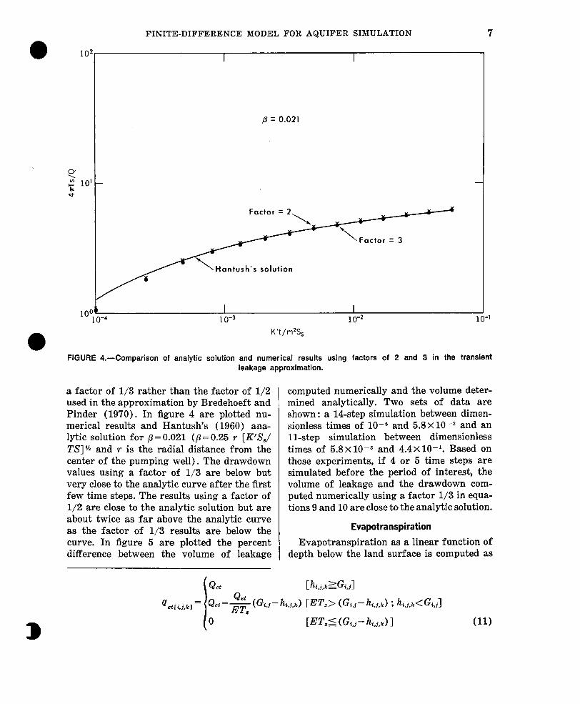
The transient parts of equations 9 and 10 are based on the analytic solutions for the flux from a confining layer resulting from an instantaneous stepwise change in head in the aquifer. The factor of l/3 appearing in dimensionless time is included in order to approximate the transient flux resulting from the actual drawdown in the aquifer. In effect the transient flux is approximated by applying a step change in head equal to the drawdown from the start of the pumping period at l/:3 of the elapsed time in the pumping period. (See fig. 3.)

The results of several numerical experiments indicate that it would be better to use

b.

solution

TIMIE SINCE PUMPING STARTED, IN THE CURRENT PUMPING PERIOD

FIGURE 3.-The total diawdown at the elapsed time, t, in the pumping period (a) is applied at t/3 in equations , 9 and 10 to approximate 9’,.,,r, the transient part of Q’w,~ (b).

c


j¶ = 0.021

Hantush’s solution

1 o-3 10-Z K’t/m2Ss

10-l

FIGURE 4.-Comparison of analytic solution and numerical results using factors of 2 and 3 in the transient leakage approximation.

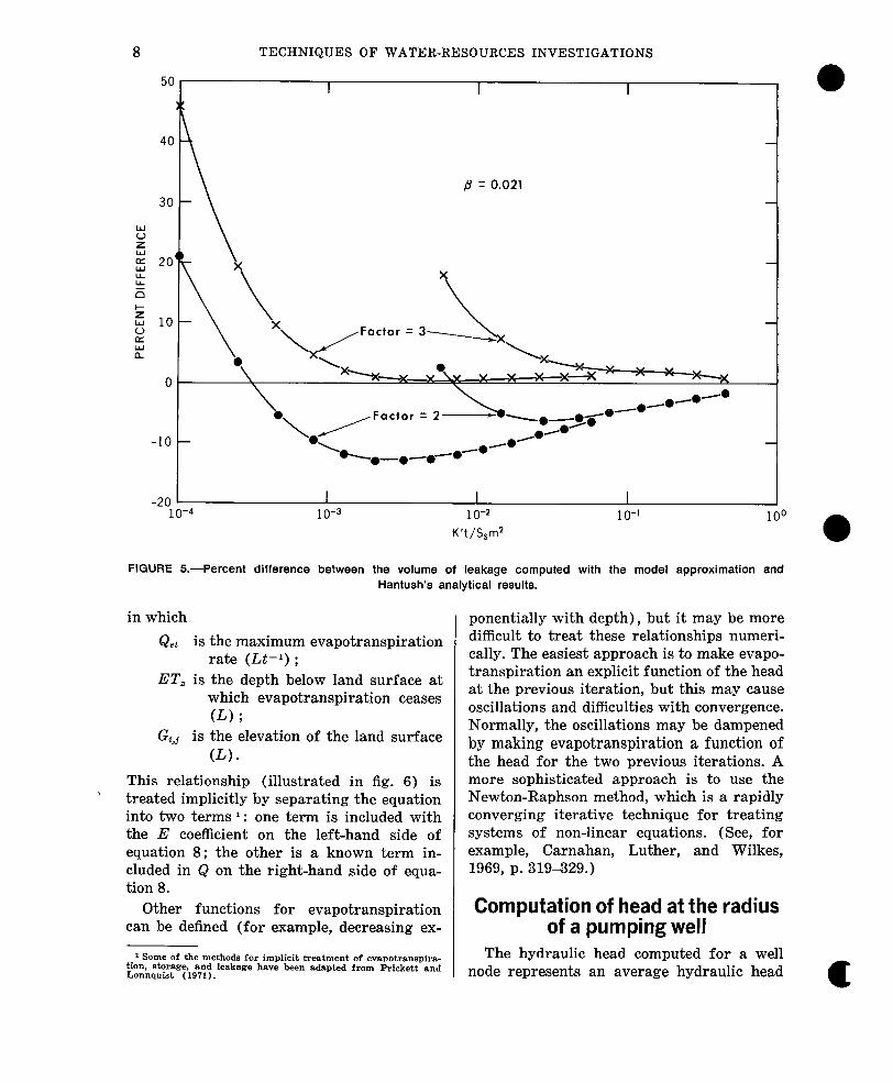
a factor of l/3 rather than the factor of l/2 used in the approximation by Bredehoeft and Pinder (1970). In figure 4 are plotted numerical results and Hantush’s (1960) analytic solution for p= 0.021 (p = 0.25 r [K’S,/ TS]U and r is the radial distance from the center of the pumping well). The drawdown values using a factor of l/3 are below but very close to the analytic curve after the first few time steps. The results using a factor of l/2 are close to the analytic solution but are about twice as far above the analytic curve as the factor of l/3 results are below the curve. In figure 5 are plotted the percent difference between the volume of leakage

computed numerically and the volume deter- mined analytically. Two sets of data are shown: a 16step simulation between dimensionless times of lo+ and 5.8x10-* and an 11-step simulation between dimensionless times of 5.8~10-~ and 4.4X 10-l. Based on those experiments, if 4 or 5 time steps are simulated before the period of interest, the volume of leakage and the drawdown computed numerically using a factor l/3 in equations 9 and 10 are close to the analytic solution.

Evapotranspiration

Evapotranspiration as a linear function of depth below the land surface is computed as

(11)

8

50

)C

0

-20 -

TECHNIQUES OF WATER-RESOURCES INVESTIGATIONS

/9 = 0.021

10-d 1 o-3 1 o-2

K’t/Ssm2 1 o-1 100

FIGURE 5.-Percent difference between the volume of leakage computed with the model approximation and Hantush’s analytical results.

in which

&et is the maximum evapotranspiration rate (U-l) ;

ET, is the depth below land surface at which evapotranspiration ceases WI ;

Gi,j is the elevation of the land surface W) *

This relationship (illustrated in fig. 6) is ’ treated implicitly by separating the equation

into two terms 1 : one term is included with the E coefficient on the left-hand side of equation 8 ; the other is a known term included in Q on the right-hand side of equation 8.

ponentially with depth), but it may be more difficult to treat these relationships numerically. The easiest approach is to make evapotranspiration an explicit function of the head at the previous iteration, but this may cause oscillations and difficulties with convergence. Normally, the oscillations may be dampened by making evapotranspiration a function of the head for the two previous iterations. A more sophisticated approach is to use the Newton-Raphson method, which is a rapidly converging iterative technique for treating systems of non-linear equations. (See, for example, Carnahan, Luther, and Wilkes, 1969, p. 319329.)

Other functions for evapotranspiration Computation of head at the radius can be defined (for example, decreasing ex- of a pumping well

1 Some of the methods for implicit treatment of evapotranspiration. storage. and leakage have been adapted from Prick&t and Lonnsuist (1971).

The hydraulic head computed for a well node represents an average hydraulic head


O- Gi,j Gi,j-ET,

DEPTH BELOW LAND SURFACE

FIGURE 6.-Evapotranspiration decreases linearly from Qet where the water table is at land surface to zero where the water table is less than or equal to GL,-ET..

Qw[i, j, k]/4

hi,j,k 0

-AX-

a

computed for the block and is not the head in a well. An option to compute the head and drawdown at a well is included in the model. This computation uses the radius, re, of a hypothetical well for which the average value of head for the cell applies. An approximat- ing equation is then used to make the extra- polation from re to the radius of a real well.

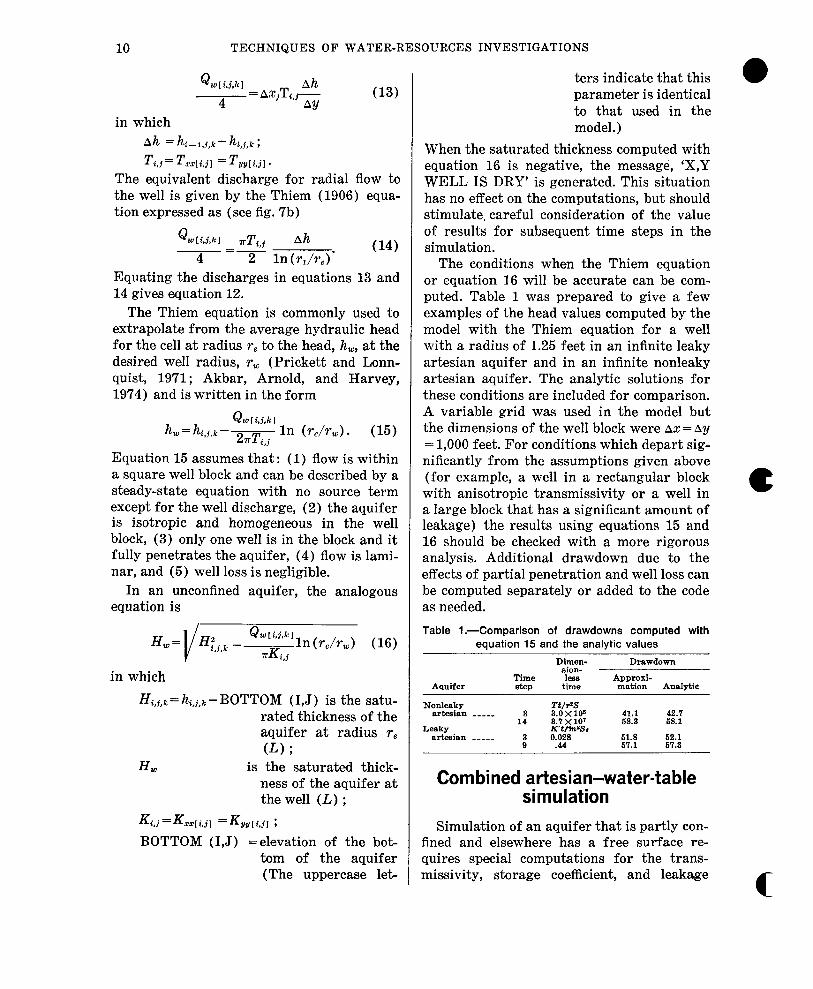
The radius re can be computed as (Prickett, 1967)

re = rJ4.81 (12) in which r1 =Axj= Ay, (fig. 7). Equation 12 assumes steady flow, no source term other than well discharge in the well block, and that the area around the well is isotropic and homogeneous. The derivation of equation 12 can be seen with reference to figure ‘7 in which the four nodes adjacent to node i,j are assumed to have head values equal to the value at node i - 1, j. In figure ‘7a one-quarter of the discharge to the well node i,j is computed by the model as

\/hi,i,k

b

3 FIGURE 7.-Flow from cell (i--l,/? to cell (Q)(a) and equivalent radial flow to well (i,n with radius r,(b).


Q urli.Lkl ah 4

= Ax~T~,~--- (13) AY

ters indicate that this 0

in which Ah = hc-l,j,k- hi,j,k ; Ti,j= Tm[i,jl = Tg,[i,jl*

The equivalent discharge for radial flow to the well is given by the Thiem (1906) equation expressed as (see fig. 7b)

Q ~1 ti,ikl T 77 i,j hh - =-- (14)

4 2 In (r&,)’ Equating the discharges in equations 13 and 14 gives equation 12.

The Thiem equation is commonly used to extrapolate from the average hydraulic head for the cell at radius re to the head, h,, at the desired well radius, rw (Prickett and Lonn- quist, 1971; Akbar, Arnold, and Harvey, 1974) and is written in the form

Qw~~.j.kI L = hi,j.k - 2nTj,j In (rehw) . (15)

Equation 15 assumes that: (1) flow is within a square well block and can be described by a steady-state equation with no source term except for the well discharge, (2) the aquifer is isotropic and homogeneous in the well block, (3) only one well is in the block and it fully penetrates the aquifer, (4) flow is lami- nar, and (5) well loss is negligible.

In an unconfined aquifer, the analogous equation is

I H,= V &J [ Likl Htjk --- , 3 J-G,

In (r&-d (16)

in which

Hi,j,k= hi,i,k - BOTTOM (1,J) is the saturated thickness of the aquifer at radius re (L) ;

HW is the saturated thickness of the aquifer at the well (L) ;

K4.j =Krnri.j, =Kgyli.jl ; BOTTOM (1,J) =elevation of the bot-

tom of the aquifer (The uppercase let-

parameter is identical to that used in the model.)

When the saturated thickness computed with equation 16 is negative, the message, ‘X,Y WELL IS DRY’ is generated. This situation has no effect on the computations, but should stimulate, careful consideration of the value of results for subsequent time steps in the simulation.

The conditions when the Thiem equation or equation 16 will be accurate can be computed. Table 1 was prepared to give a few examples of the head values computed by the model with the Thiem equation for a well with a radius of 1.25 feet in an infinite leaky artesian aquifer and in an infinite nonleaky artesian aquifer. The analytic solutions for these conditions are included for comparison. A variable grid was used in the model but the dimensions of the well block were Ax = Ay

= 1,000 feet. For conditions which depart significantly from the assumptions given above (for example, a well in a rectangular block with anisotropic transmissivity or a well in a large block that has a significant amount of leakage) the results using equations 15 and 16 should be checked with a more rigorous analysis. Additional drawdown due to the effects of partial penetration and well loss can be computed separately or added to the code as needed.

Table l.-Comparison of drawdowns computed with equation 15 and the analytic values

Aquifer Time BbP

Dimen- sionless

time

Drawdown

Approxi- mation Analytic

Nonleaky artesian _____

Leaky srteman ---_-

TtP.9 3 41.1 42.7

14 ::70::::

68.3 68.1 Iww;,

i O:E8 E:! 62.1 67.3

Combined artesian-water-table simulation

Simulation of an aquifer that is partly confined and elsewhere has a free surface requires special computations for the transmissivity, storage coefficient, and leakage

c


term. The following paragraphs describe the computations required. Some of the methods of coding these procedures have been adapted from Prickett and Lonnquist (1971).

Transmissivity

The transmissivity is computed as the saturated thickness of the aquifer times the hydraulic conductivity. This computation requires that the elevations of the top and bottom of the aquifer be specified. Where the aquifer crops out, the top of the aquifer is assigned a fictitious value greater than or equal to the elevation of the land surface.

Storage

The storage term requires special treatment at nodes where a conversion from artesian to water-table conditions, or vice versa, occurs during a time step. The program first checks for a change at a node during the last iteration. If there has been a change from artesian to water-table conditions, the storage term is

in which

SUBS = ( &i,~-l - TOP (I,J) 1

(&,j-Sy[i.jl 1 lAt ;

TOP (1,J) =elevation of the top of the aquifer.

The purpose of SUBS is to correctly appor- tion the storage coefficient and specific yield according to the relationship in figure 8a.

For a change from water-table to artesian conditions, the storage term is

g thy,,,,- hr,j,k--l) -SUBS

in which

SUBS= (hi,j,k-cTOP(I,J) 1 (Sy[i.j~ - L!&,~) /At.

SUBS subtra& the storage coefficient and adds the specific yield for the distance B illustrated in figure 8b.

Leakage

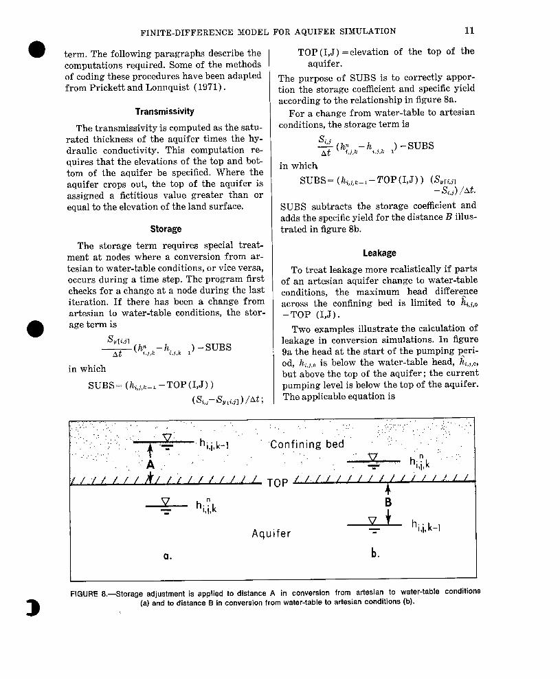
To treat leakage more realistically if parts of an artesian aquifer change to water-table conditions, the maximum head difference across the confining bed is limited to h,,j,,, -TOP (1,J).

Two examples illustrate the calculation of leakage in conversion simulations. In figure 9a the head at the start of the pumping period, hi,i,o is below the water-table head, h,,,,, but above the top of the aquifer; the current pumping level is below the top of the aquifer. The applicable equation is

,. & - 1 1. / /.k/ / / / / f /./. / ./. TOP A.‘/. r’ / / i 1 J ./ / / 1 / / 1 1 /

& bilk 9 7

Aquifer - hi,i, k-1

a. b.

FIGURE 8.--Storage adjustment is applied to distance A in conversion from artesian to water-table conditions

D (a) and to distance B in conversion from water-table to artesian conditions (b).


A V - hiiO I 1

FIGURE O.-Two of the possible situations in which leakage is restricted in artesian-water-table simulations.

“91 + TL t&,0 -TOP(I,J)).

For this situation q’c,j,k appears on the right- hand side of the difference equation and is treated explicitly. Only if both hi,j,o and h;,j,k are above the top of the aquifer is the leakage term treated implicitly by including TL in the E coefficient. This is accomplished in the code by setting U = 1.

In the second example (fig. 9b), both hi,j,o and h;,j,l, are below the top of the aquifer and the equation for leakage reduces to

K! . @i, j,k = - ,I’;&,,-TOP(I,J) 1.

If leakage across a subjacent confining bed is significant, it will be necessary to add a second leakage term. The flux described by this term will not be restricted where water- table conditions occur.

Test Problems In a subsequent section the computational

work required for solution of four test problems by the numerical techniques available in the model is analyzed. It is appropriate, however, to introduce the test problems here because they are used in the discussion of iteration parameters in the section on numerical

techniques. The problems are for steady-state conditions since the resulting set of simultaneous equations are more difficult to solve than are the set of equations for transient problems which generally involve smaller head changes. 0

For each of these problems a closure criterion was chosen to decide when a solution is obtained to the set of finite-difference equations. (See Remson, Hornberger, and Molz, 19’71, p. 185-186.) Normally, in this model, a solution is assumed if:

Max 1 hn-hn-l 1 5 E

where E is an arbitrary closure criterion (L) . For the purpose of the numerical comparisons given later in this documentation, the absolute value of the maximum residual (de fined by equation 28) is used to compare methods.

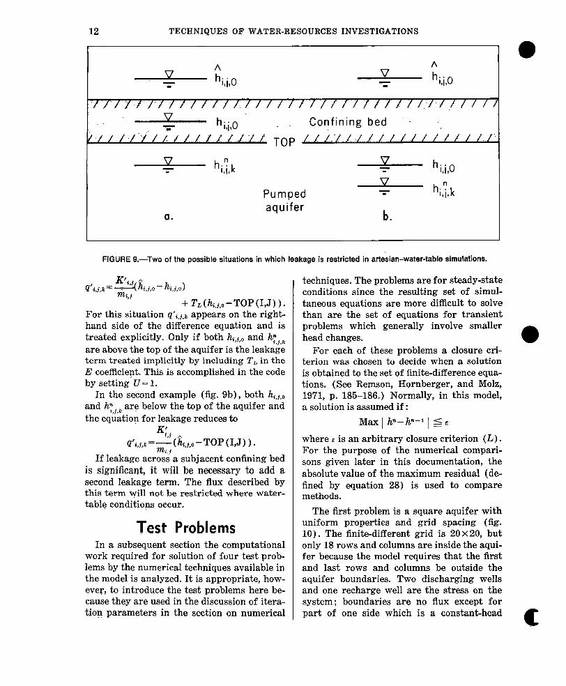
The first problem is a square aquifer with uniform properties and grid spacing (fig. 10). The finite-different grid is 20 x 20, but only 18 rows and columns are inside the aquifer because the model requires that the first and last rows and columns be outside the aquifer boundaries. Two discharging wells and one recharge well are the stress on the system ; boundaries are no flux except for part of one side which is a constant-head

c


0 PROBLEM CHARACTERISTICS

Transmlsstvlty: Txx = Tyy = 0.1 ft ‘/s (0.009m ‘/s) Grad spacing:nx =ay = 5000 ft (1500m) Dlmenslons of gnd. 18x18

I T- 0 W 20

15-

EXPLANATION OF SYMBOLS

& Constant head boundary, elevation 0 ft (0 m)

m No-flow boundary

w Dlschargmg well at 2 ft “/s (0.06 m ‘/s)

R Recharging well at 2 ft “/s (0.06 m 3/s)

-5~ Lme of equal drawdown Interval 5 ft. (15 m)

FIGURE lO.-Characteristics of test problem 1.

boundary. A closure criterion of 0.001 foot (0.0003 metre) was used.

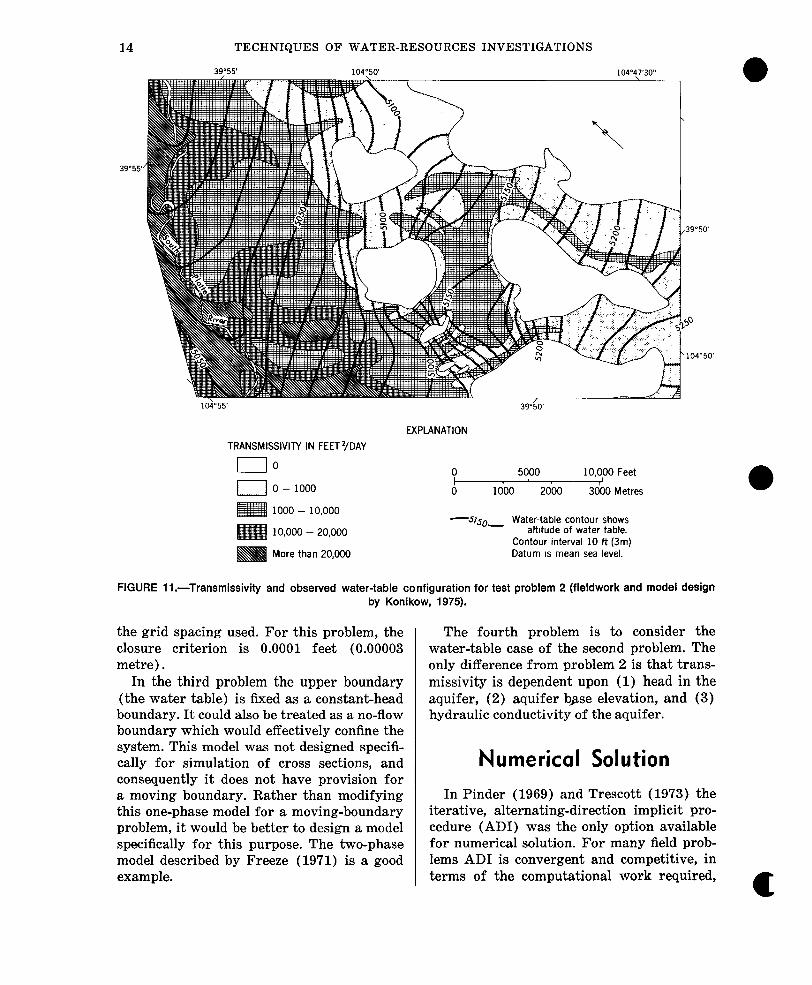
Konikow (1974) designed the second problem in his analysis of ground-water pollution at the Rocky Mountain Arsenal northeast of Denver, Cdo. It is included as one of the test problems because it is typical of many field problems and because there is some diffi- culty in obtaining a steady-state solution with the alternating-direction implicit procedure. The transmissivity distribution is shown in figure 11; note the extensive areas where the transmissivity is zero because the surficial deposits are unsaturated. The finite-difference grid representing this aquifer is 25 x38 with square blocks 1,000 feet (300 metres) on a side. The model has constantchead boundaries at the South Platte River and where the aquifer extends beyond the limits of the model; elsewhere no-flux boundaries are employed. Although this is a water-table aquifer, it is assumed for problem 2 that

transmissivity is independent of head. The model includes 49 irrigation wells and recharge from canals and irrigation. In figure 11 the observed water-table configuration is shown, and it is used as the initial surface for the simulation; the computed water table is generally within a few feet of the observed. For this problem the closure criterion is 0.001 foot (0.0003 metre).

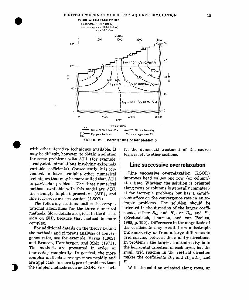
The third problem is a cross-section with three horizontal layers and other characteristics shown ,in figure 12. Transmissivity equals hydraulic conductivity for this problem because it is conceived as a slice one unit wide. The values for transmissivity are arbitrary. Note in particular that the horizontal conductivity is 100 times the vertical conductivity in all layers and that the middle layer acts as a confining layer between the upper and lower layers. The coefficients Bi,j and Hi,,, however, are 100 times greater than the horizontal coefficients Di,j and Fi,j because of


39055

TRANSMISSIVITY IN FEETZ/DAY EXPLANATION

no 0 5000 10,000 Feet

0 0 - 1000 0 ldoo 2ooo 3000 Metres

1000 - 10,000

10,000 - 20,000

More than 20,000

-~‘so, Water-table contour shows altitude of water table.

Contour interval 10 ft (3m) Datum IS mean sea level.

FIGURE Il.-Transmissivity and observed water-table configuration for test problem 2 (fieldwork and model design by Konikow, 1975).

the grid spacing used. For this problem, the closure criterion is 0.0001 feet (0.00003 metre) .

In the third problem the upper boundary (the water table) is fixed as a constant-head boundary. It could also be treated as a no-flow boundary which would effectively confine the system. This model was not designed specifically for simulation of cross sections, and consequently it does not have provision for a moving boundary. Rather than modifying this one-phase model for a moving-boundary problem, it would be better to design a model specifically for this purpose. The two-phase model described by Freeze (1971) is a good example.

The fourth problem is to consider the water-table case of the second problem. The only difference from problem 2 is that transmissivity is dependent upon (1) head in the aquifer, (2) aquifer base elevation, and (3) hydraulic conductivity of the aquifer.

Numerical Solution

In Pinder (1969) and Trescott (1973) the iterative, alternating-direction implicit procedure (ADI) was the only option available for numerical solution. For many field problems AD1 is convergent and competitive, in terms of the computational work required,

FINITE-DIFFERENCE MODEL FOR AQUIFER SIMULATION PROBLEM CHARACTERISTICS

Transmtsslwty Txx = 100 Tyy Grad spacmg AX = lOOOft (300117)

ay = 10 ft (3m)

METRES 0 1500 3000 4500 6000

1 Tyy = 10 ft (0.9m2/s)

0 0

0 6000 12000 18000

FEET

EXPLANATION

L Constant head boundary I$?%?%’ No-flow boundary

130- 135-- Equlpotentlal lines Vetilcal exaggeratm 83 1

FIGURE It.-Characteristics of test problem 3.

with other iterative techniques available. It may be difficult, however, to obtain a solution for some problems with AD1 (for example, steady-state simulations involving extremely variable coefficients). Consequently, it is con- venient to have available other numerical techniques that may be more suited than AD1 to particular problems. The three numerical methods available with this model are ADI, the strongly implicit procedure (SIP), and line successive overrelaxation (LSOR) .

The following sections outline the computational algorithms for the three numerical methods. More details are given in the discussion on SIP, because that method is more complex.

For additional details on the theory behind the methods and rigorous analysis of convergence rates, see for example, Varga (1962) and Remson, Hornberger, and Molz (1971). The methods are presented in order of increasing complexity. In general, the more complex methods converge more rapidly and are applicable to more types of problems than the simpler methods such as LSOR. For clari-

15

ty, the numerical treatment of the source term is left to other sections.

Line successive overrelaxation Line successive overrelaxation (LSOR)

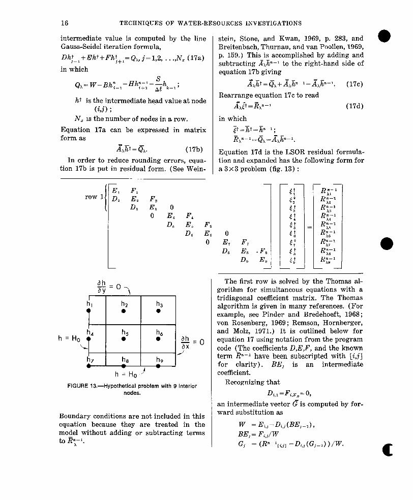
improves head values one row (or column) at a time. Whether the solution is oriented along rows or columns is generally immateri- al for isotropic problems but has a significant af%ct on the convergence rate in anisotropic problems. The solution should be oriented in the direction of the larger coefficients, either &,! and H4,, or & and Fi,j (Breitenbach, Thurnau, and van Poollen, 1969, p. 159). Differences in the magnitude of the coefficients may result from anisotropic transmissivity or from a large difference in grid spacing between the x and y directions. In problem 3 the largest transmissivity is in the horizontal direction in each layer, but the small grid spacing in the vertical direction makes the coefficients & and Hi,,r* & and Fi,+

With the solution oriented along rows, an


intermediate value is computed by the line Gauss-Seidel iteration formula,

Dh~~-l+Eh++Fh~+l=Qx,j=1,2, . . .,N, (17a)

in which

h+ is the intermediate head value at node (a ;

N, is the number of nodes in a row. Equation 17a can be expressed in matrix form as

=- A,h+ = &. (17b)

In order to reduce rounding errors, equation 17b is put in residual form. (See Wein-

h= Ho

row 1

I

E, F, D, Es F,

D, Es 0 0 E, F,

D, Es F, D, E,

0

-

0

E, F, D, E, -F,

D, Es -

i!LO av 7(

I hl

t h4 L b

stein, Stone, and Kwan, 1969, p. 283, and Breitenbach, Thurnau, and van Poollen, 1969, p. 159.) This is accomplished by adding and subtracting &%-l to the right-hand side of equation 17b giving

A,~+=~,+Ax~n-l-Ax~~-l. (I7c) Rearrange equat,ion 17~ to read

A=,@ =&n--1 (17d)

in which ~+=~+.-~w;

Equation 17d is the LSOR residual formula- tion and expanded has the following form for a 3x3 problem (fig. 13) :

hz 0

h5 0

h 0

h6 0

b

h=Ho9

FIGURE 13.-Hypothetical problem with 9 interior nodes.

Boundary conditions are not included in this equation because they are treated in the model without adding or subtracting terms to iy’.

The first row is solved by the Thomas algorithm for simultaneous equations with a tridiagonal coefficient matrix. The Thomas algorithm is given in many references. (For example, see Pinder and Bredehoeft, 1968; von Rosenberg, 1969 ; Remson, Hornberger, and Molz, 1971.) It is outlined below for equation 17 using notation from the program code (The coefficients D,.E,F, and the known term p-l have been subscripted with [i,j] for clarity). BE, is an intermediate coefficient.

Recognizing that

D,, = K,N,= 0, an intermediate vector C? is computed by forward substitution as

W = ELI-Di,j(BEj-d, BE, = F<,j,/ W Gj = (Rn-lii,jl - Di,j (G,-1) ) /W. c


0 The values of $ for row i are then computed by backward substitution as

4n approximate equation for J is 3’z~yz--1+E’i(~i+~‘i(~i+l

=R’i,i=1,2,. . .,N, (18)

n which where

since

The head values for row 1 are then computed by the equation

h;l=h;;l+cotfj,j=l,. . .,Na I I If o is 1, the solution is by the line Gauss-

Seidel formula, but convergence is slow in general. The convergence rate is improved significantly by “overrelaxation” with l<~ < 2. Discussion of the acceleration parameter is deferred until after the following section on two-dimensional correction.

Two-dimensional correction to LSOR

In certain problems, the rate of convergence of LSOR can be improved by applying a one-dimensional correction (1DC) procedure introduced by Watts (1971) or the ex- tended two-dimensional correction (2DC) method described by Aziz and Settari (1972). These methods remove the components of certain eigenvectors in the LSOR iteration matrix from the solution vector. If the eigen- values associated with these eigenvectors dominate the problem, particularly those including anisotropy, the convergence rate is greatly improved.

The 2DC method is applied after one or more LSOR iterations. The corrected head values are used as an improved starting point for the next iteration and the process is re- peated until convergence is achieved.

The two-dimensional correction for the head at (i,j) is defined as

h;;,k= htj,,+ai+ij, i= 1,. . .,N, j= 1,. . .,N,

in which

h;“,;.k is the corrected head at iteration n; ffi is the correction for row i ; h A is the correction for column j. N, is the number of nodes in a column.

H’t = - 8Hs,j ; j

An approximate equation for ,? is D’j~i--1+E’g~~+F~j~~$1=:R’i,j =1,2,. . .,N,

(19) in which

D’j= - ZDc,j; 21

E’j=X(D,,~+Fc,t+S.~ ; i At

Equations 18 and 19 are derived with the following equations

flR;;=O, i=1,2,. . .,N,

,and

i$lRy;=O, j=:l,2,. . .,N,

which force the sum of residuals for each row and each column to zero when the vector Em* is substituted into equation 8. Aziz and Set- tari (1972) give the exact equations for z and g but point out that equations 18 and 19 are good approximations and, in practice, are easier to solve. For example, equation 19, which used alone is Watts’ 1DC method, is written ‘in matrix form as


for the problem in figure 13. Equation 18 has an analogous form and both are easily solved by the Thomas algorithm.

Note that Cu and 2 in the model are zero for those rows and columns in which one or more_ constant-head nodes are located. If Cu and fi were not zero it would not be possible to maintain a constant value at the appropriate nodes. As Watts (1973) points out, therefore, the pro’cedure is most useful in simulations dominated by no-flow boundaries. For those simulations in which 2DC is useful, it is generally better to apply the corrections after several rather than after each LSOR iterac tion. After experimenting with a few problems, we have found it practical to apply 2DC after every 5 LSOR iterations.

LSOR acceleration parameter

The optimum value of o for maximum rate of convergence lies between 1 and 2 and is commonly between 1.6 and 1.9. If only one or two runs will be made on a problem, it is probably best to choose an o based on experience. If. many runs will be made, it will be worthwhile to use an o close to the optimum value. For simple problems O,Bt can be com- put,ed as explained, for example, by Remson, Hornberger, and Molz (19’71, p. 188-199) using the equation

2

w= I++p(G) (20)

in which

p(G) is the spectral radius (dominant eigen- value) of the Gauss-Seidel iteration matrix. For typical field problems it is possible to use equation 20 to estimate uopt in an iterative process if 2DC is not used. In the first simulation of the problem, set o= 1.0 and allow at least 100 iterations. In applying this method

to problems 1, 2, and 3 it took 25 iterations to arrive at mOpt for problem 2, but about 100 iterations to obtain WOpt for problem 1 and 3. Obviously this method may involve a lot of computational effort to obtain w,,~~. More efficient methods using equation 20 have been devised to update o during the iteration process. For example, Breitenbach, Thurnau, and van Poollen (1969) use a modified form of Varga’s (1962) “power method,” Carre’s (1961) method is described by Remson, Hornberger, and Molz (1971, p. 199-203)) and Cooley (1974) has a simple method for improving o for transient problems.

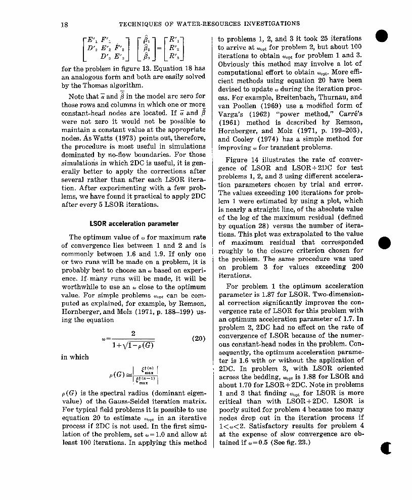
Figure 14 illustrates the rate of convergence of LSOR and LSOR+ 2DC for test problems 1, 2, and 3 using different acceleration parameters chosen by trial and error. The values exceeding 100 iterations for problem 1 were estimated by using a plot, which is nearly a straight line, of the absolute value of the log of the maximum residual (defined by equation 28) versus the number of iterations. This plot was extrapolated to the value of maximum residual that corresponded roughly to the closure criterion chosen for the problem. The same procedure was used on problem 3 for values exceeding 200 iterations.

For problem 1 the optimum acceleration parameter is 1.87 for LSOR. Two-dimensional correction significantly improves the convergence rate of LSOR for this problem with an optimum acceleration parameter of 1.7. In problem 2, 2DC had no effect on the rate of convergence of LSOR because of the numer- ous constant-head nodes in the problem. Con- sequently, the optimum acceleration parameter is 1.6 with or without the application of 2DC. In problem 3, with LSOR oriented across the bedding, Wopt is 1.88 for LSOR and about 1.70 for LSOR + 2DC. Note in problems 1 and 3 that finding Wept for LSOR is more critical than with LSOR+ 2DC. LSOR is poorly suited for problem 4 because too many nodes drop out in the iteration process if 1<0<2. Satisfactory results for problem 4 at the expense of slow convergence are obtained if 0 = 0.5 (See fig. 23.)


0

PROBFFM 1 PROBLEM 2

I I I I I

60

50

40

30

20

10

0 1.4 1.5 16 1 7 18 19 2.0 2 1.3 14 1.5 1.6 1.7 18 .9 .3 14 1.5 1.6 1.7 18 1.9 2.0

ACCELERATION PARAMETER

l LSOR computed

o LSOR extrapolated

X LSOR + 2DC every 5 iteration!

I I I I I I

I

250

I-

O-

PpOBLEM 3

I I I I I I

Alternating-direction implicit procedure

Peaceman and Rachford (1955) described the iterative, alternating-direction implicit procedure for solution of a steady-state (La- place) equation in two space dimensions. This procedure, however, is equally applicable to transient problems where it has the advant- age of allowing larger time steps than can be used with non-iterative ADI. (Non-iterative AD1 was used by Pinder and Bredehoeft, 1968.) In the AD1 technique, two sets of matrix equations are solved each iteration. The equations for row,s in which head values along rows are computed implicitly and those along columns are obtained from the previous column computations are defined as

Dh;I;h + E,.h”- % + Fh-f” =Q,,j=1,2,. . .,N, (21a)

in which

E,= - (D+F+;t+Mr) ;

FIGURE 14.-Number of iterations required for solution by LSOR and LSOR + 2DC using different acceleration parameters.

Qr= -Bhy~"_-,' + (B+H-A&)h"+'

-f&n-'- shx-l+ W; ‘+l At

M1 is the iteration parameter ; 1 is the iteration parameter index.

In matrix form equation 21.a is ~Jp-% = QT. @lb)

To put equation 21b in residual form, add and subtract A&+-l to the right-hand side giving

~~~*-~=a-~~~~-l+A=,~~-l (21c)

Rearrange equation 21~ to read : A=,p-n =j&n-1 GW

in which F”-‘/z=j+,L~n-1; &n-1=(&A=,+.

Equation 21d is the AD1 row formula in residual form. Its matrix form is the same as that for equation 17d and is solved for each row by the Thomas algorithm. To complete the first half of the AD1 iteration, Em-n is computed by


The equations in which head values along columns are considered implicitly and those along rows explicitly are written as : Bhin_l+E,h”+Hh~+I=&,,i=1,2,. . .,N, (22a)

in which

E,= - (B+H+;+il&) ;

&,= -Dh;y;h + (D+F-M,)hn-‘h

-Fhyy -;h,-,+ 74’.

Equation 22a in matrix form is z,iP= &. Wb)

By adding and subtracting ~&-~ to the right-hand side of equation 22b, it can be put in the residual form

&+~,n-$4; WC) in which

P =j+-j+M. j&n-M q&~&M.

Equation 22~ is solved for each column by the Thomas algorithm, and the vector @ for each row is obtained by the equation

j&j+%+f.

A set of iteration parameters is computed by the equation

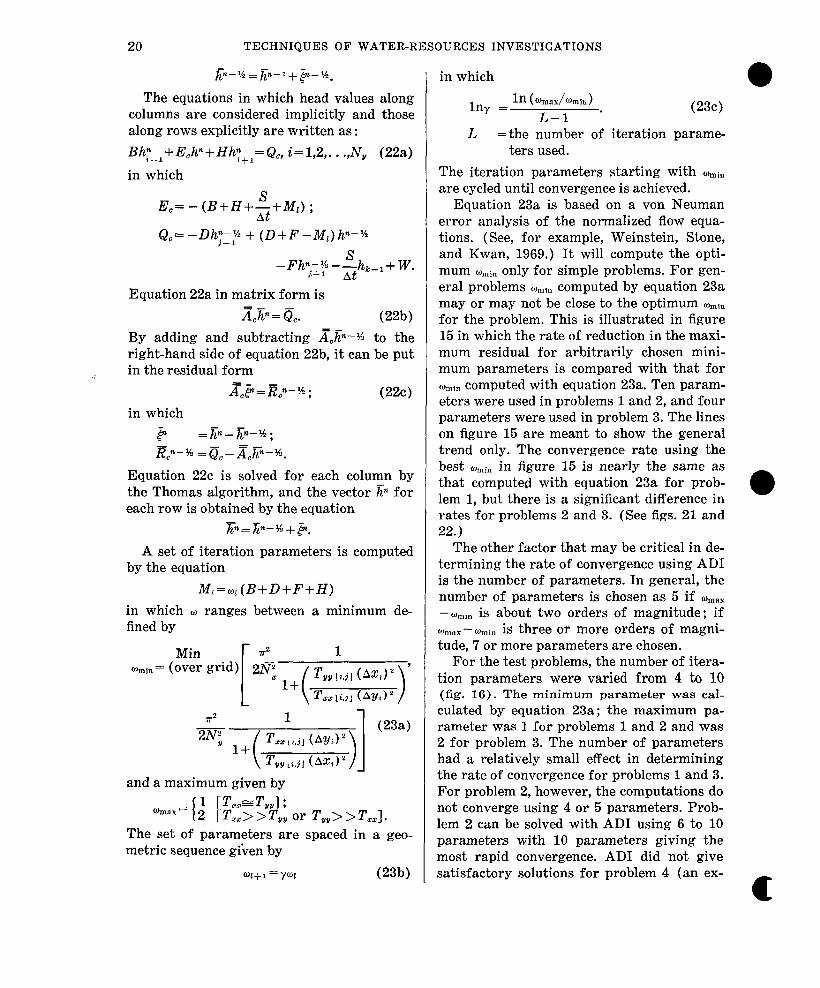
M,=w, (B+D+F+H) in which ,,, ranges between a minimum defined by

Min x2 1 wmin= (over grid) 2p

?+ TM/ [t.j~ (Ax,)’ ’ T,, [i,:~ (4-h) ’

2

G 1 (23a)

u 1+ T z.n :z,j~ (W) ’ T uu to1 (Ax,)’

and a maximum given by

%lax = I 1 IT,,=T,,l; 2 [T,,>>T,, or T,,>>T,,l.

The set of parameters are spaced in a geo- metric sequence given by

w+1=yw Wb)

in which

ln Y

= In (%d%xia) I _ (23~) L-l

L =the number of iteration parameters used.

The iteration parameters starting with wmilr are cycled until convergence is achieved.

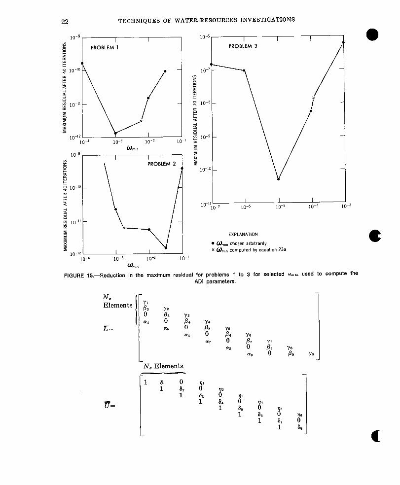
Equation 23a is based on a von Neuman error analysis of the normalized flow equations. (See, for example, Weinstein, Stone, and Kwan, 1969.) It will compute the optimum CO,in only for simple problems. For general problems %lin computed by equation 23a may or may not be close to the optimum %in for the problem. This is illustrated in figure 15 in which the rate of reduction in the maximum residual for arbitrarily chosen minimum parameters is compared with that for wnin computed with equation 23a. Ten parameters were used in problems 1 and 2, and four parameters were used in problem 3. The lines on figure 15 are meant to show the general trend only. The convergence rate using the best qnir, in figure 15 is nearly the same as that computed with equation 23a for problem 1, but there is a significant difference in 0

rates for problems 2 and 3. (See figs. 21 and 22. )

The other factor that may be critical in determining the rate of convergence using AD1 is the number of parameters. In general, the number of parameters is chosen as 5 if %ml - wmm is about two orders of magnitude ; if wmax -timin is three or more orders of magnitude, 7 or more parameters are chosen.

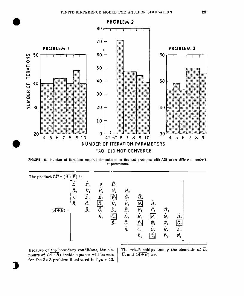
For the test problems, the number of iteration parameters were varied from 4 to 10 (fig. 16). The minimum parameter was calculated by equation 23a ; the maximum parameter was 1 for problems 1 and 2 and was 2 for problem 3. The number of parameters had a relatively small effect in determining the rate of convergence for problems 1 and 3. For problem 2, however, the computations do not converge using 4 or 5 parameters. Prob- lem 2 can be solved with AD1 using 6 to 10 parameters with 10 parameters giving the most rapid convergence. AD1 did not give satisfactory solutions for problem 4 (an ex-

c


cessive number of nodes always drop out of the solution) and, consequently, no results for problem 4 are shown in figure 16.

steady state should be achieved within a reasonable number of time steps with rapid convergence at each time step.

Strongly implicit procedure

When difficulties occur with AD1 in steady- state simulations, rather than experimenting with the critical minimum parameter or the number of parameters, it may be worthwhile to make the simulation a transient problem. In effect, S/At is used as an additional iteration parameter. If the storage coefficient is not made too large or the time step too small, ) XL=&

The set of equations (corresponding to equation 8) for the 3 x 3 problem in figure 13 may be expressed in matrix form as

(24)

L

Direct solution of equation 24 by Gaussian elimination usually requires more work and

0 computer storage than it,erative methods for problems of practical size because A’ decom- poses into a lower triangular matrix with non-zero elements from B to E in each row and an upper triangular matrix with non- zero elements from E to H in each row. All of these intermediate coefficients must be computed during Gaussian elimination, and the coefficients in the upper triangular matrix must be saved for backward substitution.

To reduce the computation time and storage requirements of direct Gaussian elimination, Stone (1968) developed an iterative method using approximate factorization. In this approach a modifying matrix B is added - to A’ formi’ng (A + B) so that equation 24 becomes

(A+B)K=Q+EE. (25)

(A-) can be made close to x but can be factored in2 the product of a lower triangular matrix L and an upper triangular matrix r, each of which has no more than three non- zero elements in each row, regardless of the size of N, and N,. Therefore, if the right- hand side of equation 25 is known, simple

recursion formulas can be derived, resulting in a considerable savings in computer time and storage. This leads to the iteration scheme --

(A+B)Iz”=~+B@-~. (26) In order to transform equation 26 into a residual form, K&l is subtracted from both sides giving --

(A+B)k=&’ (27) in which

P ,~n-~n-1. p-1 = Q- ~j&l. (2~)

The iterative scheme defined by equation 26 or 2’7 is closer to direct methods of solution (more implicit) than AD1 (hence the term strongly implicit procedure or SIP). The SIP algorithm requires (1) relationships among - the elements of z, g and (A + B) defined by rules of matrix multiplication for the equation

,? v’= (AT), and (2) relationships among the elements of Kand (Ax).

E and g have the following form for a general 3 x 3 problem (much of the notation is adapted from Remson, Hornberger, and Molz, 1971) ;


10-g I I

2 0 PROBLEM 1

k

1o-4 10-3 10-2 1

0 ml,”

0-l

I I I PROBLEM 3

I I Ej PROBLEM 2

‘4 J

2 lo-‘0 -

. 1 O-“li

\ x

EXPLANATION

l O,,, chosen arbttrarlly

I I X &,, computed by equahon 23a

10-3 10-Z 10-I 0 ml”

FIGURE 15.-Reduction in the maximum residual for problems 1 to 3 for selected w,$, used to compute the ADI parameters.

N, Elements

I

N, Elements .

‘1 i1

0

:

F Y7 a9 pas ‘p” 9 Y9

c


PROBLEM 1

--I

4 5 6 7 8 910

PROBLEM 2

8or--- 70 -

60 -

50 -

40 -

30 -

20 -

10 -

0’ 4* 5* 6 7 8 9 10

NUMBER OF ITERATION PARAMETERS *ADI DID NOT CONVERGE

PROBLEM 3

6ol----l

50

40

30 456789

FIGURE 16.-Number of iterations required for solution of the test problems with ADI using different numbers of parameters.

The product ~?a= (AT) is

(A+B)=

Because of the boundary conditions, the ele- The relationships among the elements of z, ments of (AT) inside squares will be zero

- g,and (A+B) are

B

for the 3x3 problem illustrated in figure 13.


a =B (3W

a&-l & (30b)

P =fi (3Oc)

y+“~~-1+p6,-1 =JG WW

YS =@ We)

l&V-l =@ Wf)

Yrl =g wk) where the i and j subscripts refer to the location on the model grid, not in matrix (A-).

In order to use equations 30a-30g as the basis of a numerical technique for solving equation 24 efhciently by eliminationLrela- tionships between the elements of A and - (A+B) must be defined. One possibility is to let the elzments_correspond exactly and ig- nore the C and G diagonal in (AT). Stone (1968)) however, found that this could not be used as the basis of a rapidly convergent iterative procedure. Instead, he defined a family of modified matrices starting with 30b and 30f. -

Then the other elements of (A + B) can be defined as=equal to the corresponding ele; men+ in A plus a linear combination of C and G. For example

in which $I and & are constants depending on the problem being solved.

What aze appropriate linear cosbinations of C and G with the elements of A? If equation 27 is written for node (i,j) , non-zero coefficients appear not only for the unknowns in the original difference equation but also for qmlj+* and c+li--l. This is illustrated in figure 17. To minimize the effects of the terms introduced in forming the modified matrix equation, E@ for the node (i,j) is defined as

~[~-lj+l-d~-l+r;+l -P)l +&$+*j-l-w(ty-l +q+,-ml (31)

where the terms in parentheses are second- order correct approximations for &.l.i+l, and &+l,j-l, respectively. (See Remson, Horn- berger, and Molz, 1971, p. 226, for derivation of these approximations.) To consider these terms good approximations to &i-l,i+l and

i-l X

I B

i+l z

j-l

A 0 X

T j j+l

FIGURE 17.-Coefficients of unknowns in equation 27.

t D+l,j--l an iteration parameter, 0, is added. The value of o ranges between 0 and 1, and its computation is discussed at the end of this section.

With the definition of E (31)) the iteration 0 scheme (equation 27) becomes

Bq-l+D~-l+~$+J’~+, +Hq+, +erq, i+,-“(~~~~~~+,-F)l+~~~+, j-, -4q-1+q+1 -P)] =R”-’ ’ (3%

Collecting coefficients in equation 32 associated with the nodal positions in the original difference equation gives the desired linear combinations of I? and 8 with the elements of x that define the remaining ele- - ments of (A+B) :

i?=B--wi? @a)

6=0-d (33b)

Jii=E+k+c12 (33c)

k=F-k W-W

ii=H-d We)

The coefficient 2 is obtained explicitly by combining equations 33a, 30a, and 30b as

& &-lB

l+osi-l’ @da)

a


0

Finally combining equation 33b and equations 3Oc and 30f gives

,A= V-ID 1+07]j-1.

Wb)

Equations 34, 33 and 30 (in that order) are the first part of the SIP algorithm.

Equation 28 written for node (i,j) is Rn-l=Q- (Bh;:;+Dh”-1 j-1

+Eh”-l+Fhy-;+Hhy-;).

As in the Thomas algorithm, the vector p is obtained by a process of forward and backward substitution. Combining equations 27 and 29 gives

~@=j+-l (35) Define an intermediate vector F by

@kp. (36) Then equation 35 becomes

~~=~?A~ (37) vn is first computed by forward substitution. This can be seen by writing equation 37 for node (i,j) :

0 aV;-, +/3V;~,+uVn=R”-’

or V”= (Rn-l-~V1_l-BV~_l)/Y.

The vector F may then be computed by backward substitution. Equation 36 for node (i,j) is

or P= V”-~~+, -‘1q+,.

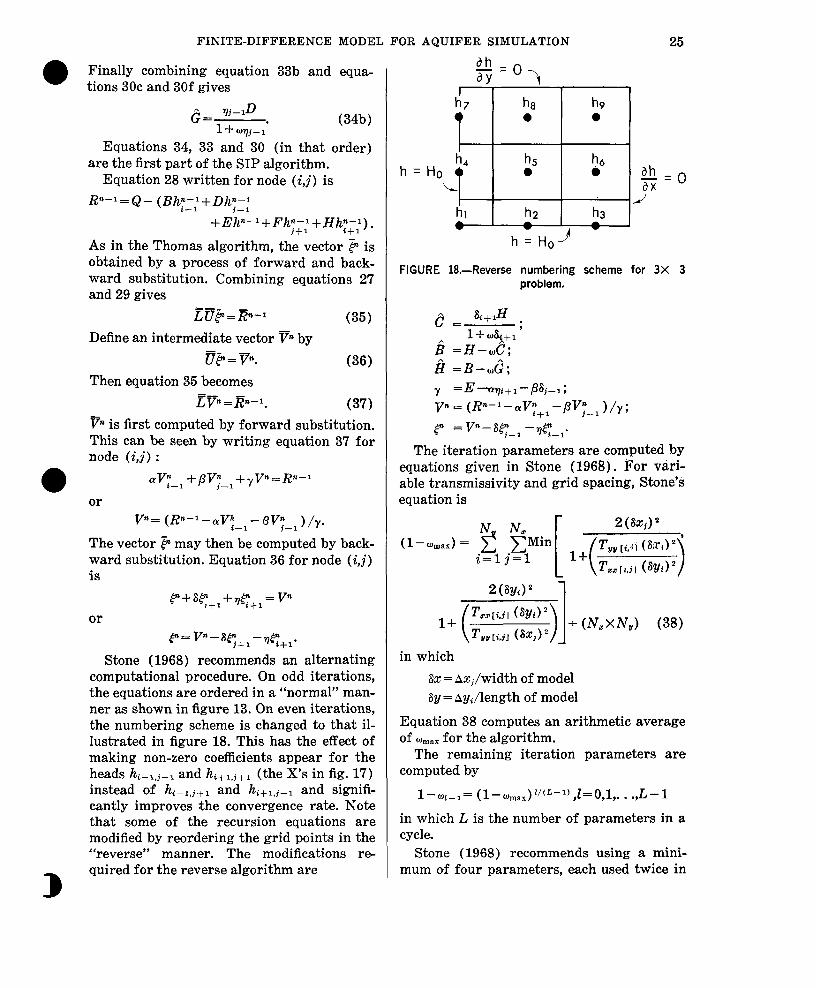
Stone (1968) recommends an alternating computational procedure. On odd iterations, the equations are ordered in a “normal” manner as shown in figure 13. On even iterations, the numbering scheme is changed to that illustrated in figure 18. This has the effect of making non-zero coefficients appear for the heads hi-1,j-1 and hi+l,j+l (the X’s in fig. 17) instead of hg-l,j+l and hi+l,j-l and significantly improves the convergence rate. Note that some of the recursion equations are modified by reordering the grid points in the “reverse” manner. The modifications re-

3

quired for the reverse algorithm are

FIGURE 18.-Reverse numbering scheme for 3X 3 problem.

Y =E -yYr]i+l-PSj--1;

vn = (R”-‘-aV;+, -P’;-, )/y;

p =vn-SC+, -7#- -

The iteration paramiteis are computed by equations given in Stone (1968 j. For variable transmissivity and grid spacing, Stone’s equation is

in which EX = AXj/width of model 6y = AyJength of model

Equation 38 computes an arithmetic average Of Oman for the algorithm.

The remaining iteration parameters are computed by

l- q+1= (l-wmax)~~(~-~),z=O,l,. . .,L-1

in which L is the number of parameters in a cycle.

Stone (1968) recommends using a minimum of four parameters, each used twice in


succession, starting with the largest first. Weinstein, Stone, and Kwan (1969)) however, indicate that it is not necessary to start with the largest parameter first or to repeat them.

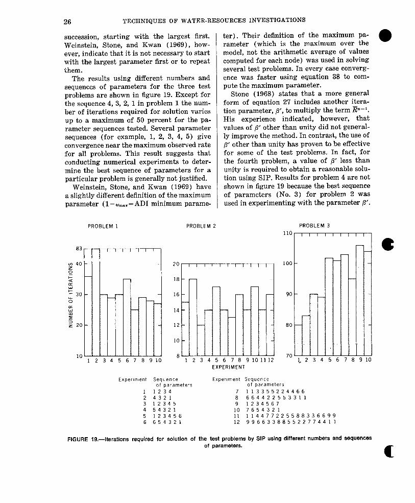
The results using different numbers and sequences of parameters for the three test problems are shown in figure 19. Except for the sequence 4, 3, 2, 1 in problem 1 the number of iterations required for solution varies up to a maximum of 50 percent for the parameter sequences tested. Several parameter sequences (for example, 1, 2, 3, 4, 5) give convergence near the maximum observed rate for all problems. This result suggests that conducting numerical experiments to deter- mine the best sequence of parameters for a particular problem is generally not justified.

Weinstein, Stone, and Kwan (1969) have a slightly different definition of the maximum parameter (1 - wII1.= = AD1 minimum parame-

PROBLEM 1

- 5 6

~ 7 8 91

ter). Their definition of the maximum parameter (which is the maximum over the model, not the arithmetic average of values computed for each node) was used in solving several test problems. In every case convergence was faster using equation 38 to compute the maximum parameter.

Stone (1968) states that a more general form of equation 27 includes another iteration parameter, p’, to multiply the term En-l. His experience indicated, however, that values of p’ other than unity did not generally improve the method. In contrast, the use of /3’ other than unity has proven to be effective for some of the test problems. In fact, for the fourth problem, a value of p’ less than unity is required to obtain a reasonable solution using SIP. Results for problem 4 are not shown in figure 19 because the best sequence of parameters (No. 3) for problem 2 was used in experimenting with the parameter p’.

PROBLEM 2

110

18

16

8 r I

Experiment Sequence of parameters

1 1234 2 4321 3 12345 4 54321 5 123456 6 654321

i iii, 3 4 5 6 7

90

80

PROBLEM 3

IIIIIlIIIl

EXPERIMENT

Experiment Sequence of parameters

7 113355224466 8 664422553311 9 1234567

10 7654321 11 114477225588336699 12 996633885522774411

7 8 9 10

FIGURE 19.4terations required for solution of the test problems by SIP using different numbers and sequences of parameters.

c


Comparison of Numerical Results

The rate of convergence using different numerical tech’niques for solving the test problems is compared in figures 20 to 23. The best results from the experiments with each iterative technique are used in the comparisons. Two curves (except for fig. 23) are shown for SIP : one with the parameter ,R’= 1 and the other with the best rate of convergence for p’#l. The sequence of w parameters is the same for both curves. Two curves are also shown for ADI: one in which the minimum parameter was calculated with equation 23a (indicated by an asterisk in the figures) ; the other with the best minimum parameter shown on figure 15.

In figures 20 to 23 the absolute value of the maximum residual for each iteration is plotted versus computation time where one unit of work is equal to the time required to complete one SIP iteration. Relative work per iteration is about 1 for ADI, 0.6 for LSOR, and 0.8 for LSOR+2DC. The maximum reb sidual for SIP and AD1 fluctuates from a maximum to a minimum over each cycle of parameters. For clarity, the curves connect the local minima for these two methods. Com- parisons in figures 20-23 should be made on the basis of the horizontal displacement of the curves, not on the basis of the termina- tion of the curves. This is similar to the type of comparisons made by Stone (1968).

Figure 20 shows the results for problem 1 (10 parameters for ADI, O= 1.87 for LSOR, o = 1.7 for LSOR + 2DC, parameter sequence, 1,1,3,3 5 5 2 2 4 4 6 6 for SIP). Of the se- 99,99,,,, quence of p’ parameters tried, the minimum work required to reduce the residual is obtained with p’ = 1.4, but this is only moder- ately better than using p/=1.0. ADI converges as rapidly as SIP for the first cycles of iteration, but from that point on converges slower than the other iterative techniques. The two AD1 curves show about the same rate of convergence for this problem. Next to SIP, LSOR+ZDC is most attractive for

D this problem.

1 o-7 I I I I

0 10 20 30 40 50 COMPUTATIONAL WORK

(Number of SIP Iterataons)

FIGURE PO.-Computational work required by different iterative techniques for problem 1.

The results for problem 2 are shown in figure 21 (10 parameters for ADI, O= 1.6 for LSOR and LSOR + 2DC, parameter sequence 1,2,3,4,5 for SIP). SIP requires the least amount of work for this problem (using p’#l.O does not significantly reduce the work required). LSOR and AD1 using the best omi,, from figure 15 are competitive with SIP. AD1 using q,,in computed with equation 23a requires about twice as much computational work. LSOR and LSOR+2DC take the same number of LSOR iterations so that the extra work required for 2DC is wasted for this problem,

In figure 22, the results using 4 parameters for ADI, the parameter sequence 1,2,3,4 for SIP, o= 1.88 for LSOR and w=1.70 for LSOR+2DC are plotted for problem 3. In this problem LSOR (with solution lines oriented along columns), AD1 with *in computed with equation 23a, and SIP with p’= 1 are competitive. Convergence is significantly improved by adding 2DC to LSOR, choosing the best omin from figure 15 for AD1 and let- ting p’ = 1.5 with SIP.


\ I I

10 I5 20

COMP”TATlONAL WORK (Number Of SIP Iterations)

FIGURE 21 .-Computational work required by different iterative techniques for problem 2.

FIGURE 22.-Computational work required by different iterative techniques for problem 3.

The results for problem 4 are shown in figures 23 and 24. The o iteration parameter sequence for SIP is 1,2,3,4,5, and the two- dimensional correction is applied every fifth iteratinn for LSOR+ 2DC. Konikow (oral

u 10 20 30 40 50

COMPUTATIONAL WORK (Number of SIP Iteratms)

FIGURE 23.-Computational work required by dlfferent iterative techniques for problem 4.

50

l-

/- 10 I b. 2 0.3 0.4 0.5 0.6 0.7 0.8

P’

I I I I

1 - 3 nodes dropped 2 - 4 nodes dropped

1

-lJ 1

2 2

I I I

FIGURE 24.-Number of iterations required for solution of problem 4 by SIP using different values of P’.


0

commun., 1975) was unable to obtain a solution to problem 4 using AD1 due to oscillations that eliminated nodes that should have been in the solution. This problem occurred not only with AD1 but also with LSOR and LSOR+ 2DC with ~>0.6 and with SIP with p’~O.6. The oscillations are apparently caused in part by the nonlinearities of the water-table problem and the necessity to cal- culate transmissivity at the known iteration level. In a water-table simulation the transmissivity is set to zero and nodes are dropped from the aquifer if the computed head is bet low the base of the aquifer. For problem 4, at least 3 nodes should be dropped with the initial conditions used.

A solution to problem 4 in which 3 to 4 nodes are dropped is obtained with LSOR and LSOR + 2DC when w= 0.5 at the expense of slow convergence. Clearly the most suitable method for this problem is SIP with p’90.6 (fig. 23). In effect the use of p’<l for SIP and 0<1 for LSOR represents “under- relaxation” and has the effect of dampening oscillations of head from one iteration to the next. This reduces the tendency for incorrect delet,ion of nodes from the solution.

Solution of problem 4 emphasizes the ad- vantage of the extra SIP iteration parameter. The optimum value of p’ inferred from figure 24 is about 0.5. Note in figure 24 that an addit,ional node is dropped for p’=O.5 and 0.6. However, the effect of this node on the remainder of the solution is negligible. For p’>O.6, either convergence was not obtained or excessive numbers of nodes were dropped for those cases that did converge.

The numerical experiments included in this report support the general conclusions of Stone (1968) and Weinstein, Stone, and Kwan (1969) that SIP is a more powerful iterative technique than AD1 for most problems. SIP is attractive, not only because of its relatively high convergence rates but because it is generally not necessary to conduct numerical experiments to select a suitable sequence of parameters. SIP has the disad- vantage of requiring 3 additional N,X N,

B arrays.

For the first three problems examined here, AD1 is a slightly better technique than LSOR when “mill near the optimum is used. Al- though this result agrees with Bjordammen and Coats (1969) who concluded that AD1 is superior to LSOR for the oil reservoir problems they investigated, it is deceptive because less work is required to obtain mopt for LSOR than is required to find the best umin for AD1 by trial and error. Furthermore, LSOR is clearly superior to AD1 in application to problem 4 where a solution was not possible with AD1 as used in this simulator.

LSOR + 2DC seems to be particularly useful with problems dominated by no-flux boundaries. The correction procedure can significantly improve the rate of convergence of LSOR even in problems such as problem 3 where all pj are zero and non-zero (Y~ occur for the lower half of the model only.

Considerations in Designing on Aquifer Model

Boundary conditions An aquifer system is usually larger than

the project area. Nevertheless the physical boundaries of the aquifer should be included in the model if it is feasible. Where it is im- practical to include one or more phy&al boundaries (for example, in an alluvial valley that may be several hundred miles long) the finite-difference grid can be expanded and the boundaries located far enough from the project area so that they will have negligible effect in the area of interest during the simulation period. The influence of an artificial boundary can be checked by comparing the results of two simulation runs using different artificial boundary conditions.

Boundaries that can be treated by the model are of two types: constant head and constant flux. Constant-head boundaries are specified by assigning a negative storage coefficient to the nodes that define the constant- head boundary. This indicates to the program that these nodes are to be skipped in the computations.

chapter cl finite-difference model for 0 … · techniques of water-resources investigations of the...

Documents