chapter 3users.dsic.upv.es/~jlinares/grafics/chapter 3.pdf · computer graphics tema 3. ... – the...

Tema 3. Transformaciones 2D 1Computer Graphics Chapter 3. 2D Transformations 1

Chapter 3Chapter 3

Chapter 3. 2D Transformations3.1 Introduction3.2 2D Transformation3.3 Composing transformations3.4 Geometric transformations around a point3.5 Coordinate system transformations


3.1 Introduction

• The model to visualize is on 2D or 3D geometric space

• Geometric transformations are generally compulsory in order to visualize our model into a device

• Geometric transformations are also compulsory in CAD systems, simulation, computer games etc.

• The transformations we are going to study are: translation, rotation and scaling


3.1 Introduction

2D and 3D coordinate systems

Y

Point at (2,-2,2)

R3

Right-handedcoordinate system

Z

X

Point at (2,3)R2

Y

X


3.1 Introduction

Y

Operation to movesum 5 to x, sum 4 to y

R2

X

Here=(2,3)

There=(7,7)

An example of geometric transformation


3.1 Introduction

• How can relate different objects?– Object position can be considered

respecting a central reference point called origin

– A vector indicates which is the direction to follow from origin and the path length to reach the point

• Notation: row or column – Ex.: the vector pointing to the center of

the car

• We will use column notation and transformation matrices will be pre-multiplied

X

Y

(2,3)(10,2)

(8,7.5)

⎥⎦

⎤⎢⎣

⎡2

10[ ]210


3.1 Introduction

• Vectors are used in computer graphics to:– Represent vertices positions– Determine a surface orientation

• Surface normal vector– Model light interaction

• Light vector

L

N

θγ

L’

N


3.1 Introduction

Sum of vectors

X

Y

P

P’

P+P’Y

X

⎥⎦

⎤⎢⎣

⎡=

32

P

⎥⎦

⎤⎢⎣

⎡=

24

P'

⎥⎦

⎤⎢⎣

⎡=⎥

⎦

⎤⎢⎣

⎡+⎥

⎦

⎤⎢⎣

⎡=+=

56

24

32

P'P'P'


3.1 Introduction

• Product by a scalar• Linear dependency

– Two vector are linearly dependents when one is multiple of the other

X

Y

-P

2P

P

αPY

X

⎥⎦

⎤⎢⎣

⎡=⎥

⎦

⎤⎢⎣

⎡=

23

yx

P

⎥⎦

⎤⎢⎣

⎡=⎥

⎦

⎤⎢⎣

⎡⋅⋅

=⎥⎦

⎤⎢⎣

⎡=

46

2232

2y2x

P2


3.1 Introduction

• Base vectors of the plane– The unit vectors (of length 1) in x and y axes are called standard base vectors of

the plane– The collection of all the scalar multiples of [1 0] give us the first coordinate axis– The collection of all the scalar multiples of [0 1] give us the second coordinate

axis• Non-orthogonal base vectors

– Can we get any [n m] vector as a combination of two arbitrary vectors [a b] and [c d]?

– It is always possible to find α and β meanwhile [a b] and [c d] do not be linearly dependents

⎥⎦

⎤⎢⎣

⎡⋅+⋅⋅+⋅

=⎥⎦

⎤⎢⎣

⎡⋅+⎥

⎦

⎤⎢⎣

⎡⋅=⎥

⎦

⎤⎢⎣

⎡dbca

ba

mn

βαβα

βαdc


3.1 Introduction

• Algebraic properties of vectors:– Commutative

• P + Q = Q + P– Associative

• (P + Q) + R = P + (Q + R)– Identity (sum)

• There is a vector 0 / (P+0)=(0+P)=P for all P

– Reverse• For any P exists a vector

-P / P + (-P) = 0

– Distributive (vector):• r (P+Q)=rP+rQ

– Distributic (scalar):• (r + s)P=rP+sP

– Associative (scalar): • r(sP)=(rs)P

– Identity (product): • For the real number 1,

1P=P for all P


3.1 Introduction

• Dot product of two vectors– The result is a scalar– Defines the length of a vector

(P*P)=x2 + y2 is the square of the length

– Allows to normalize vectors• The norm of a vector is its length• The vector is unitary if |P|=1• To normalize: P/|P|

– Measures the angles between two vectors

• If P and P’ are different of 0 then P*P’ = |P||P’|cos(θ−φ)

P

P’θ

φ

(θ−φ)

|P|sinθ

|P|cosθ

P

y'yx'xy'x'

yx

P'P ⋅+⋅=⎥⎦

⎤⎢⎣

⎡•⎥⎦

⎤⎢⎣

⎡=•

PPP •=+


3.1 Introduction

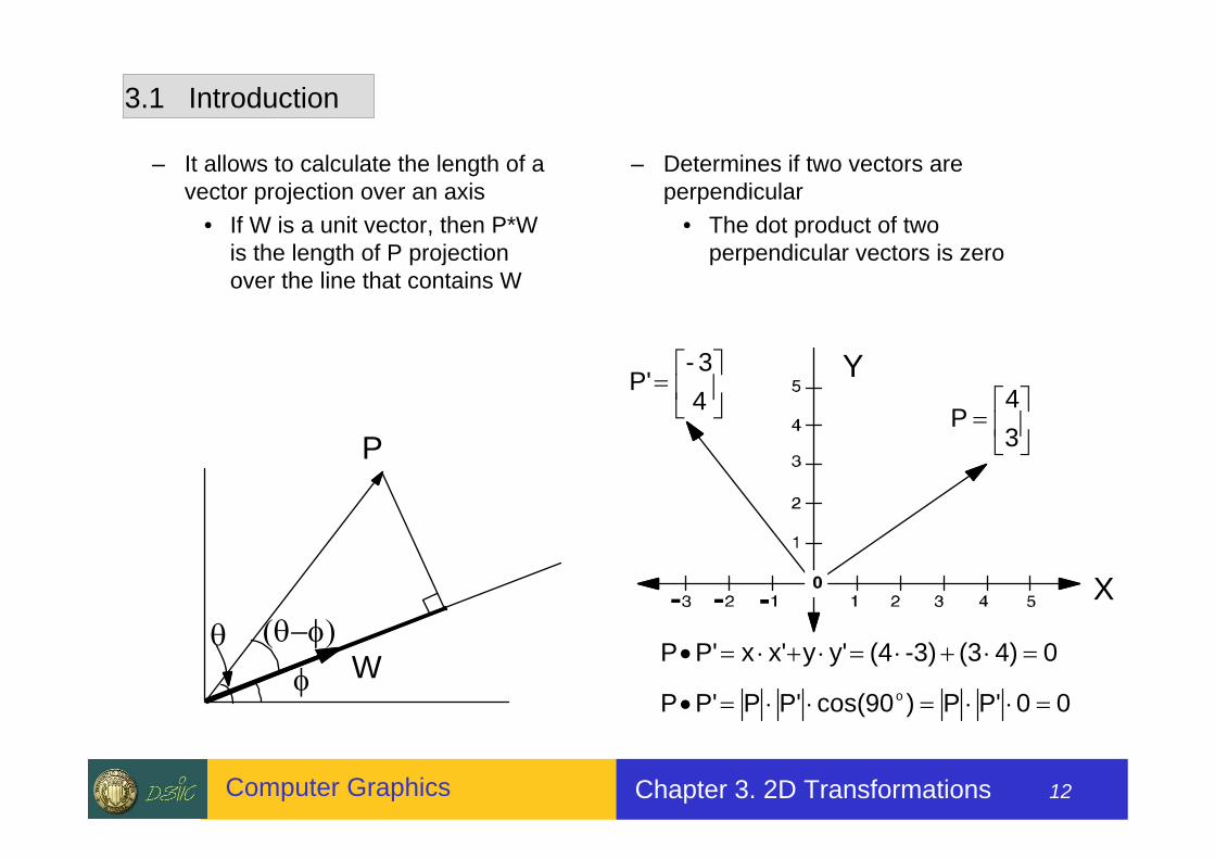
– It allows to calculate the length of a vector projection over an axis

• If W is a unit vector, then P*W is the length of P projection over the line that contains W

– Determines if two vectors are perpendicular

• The dot product of two perpendicular vectors is zero

P

Wθ

φ

(θ−φ)

⎥⎦

⎤⎢⎣

⎡=

43-

P'

⎥⎦

⎤⎢⎣

⎡=

34

P

Y

X

04)(3-3)(4y'yx'xP'P =⋅+⋅=⋅+⋅=•

00P'P)cos(90P'PP'P o =⋅⋅=⋅⋅=•


3.1 Introduction

• Cross product– The result is a vector (orthogonal to the

two input vectors)– Measures the angle between two vectors

• If P and P’ are different to 0 then |PxP’|= |P||P’|sen(θ−φ)

– Allows to calculate the point-to-line distance

• If W is a unit vector, then |PxW| is the distance from P to the line that contains W

– Determine is two vectors are parallel• The cross product modulus of two

parallel vectors is 0

z'y'x'zyxkji

P'P

→→→

=×

P

P’θφ

(θ−φ)

P

Wθ

φ(θ−φ)


3.2 2D Transformations

• 2D Points: as column vectors

• Transformations: square matrices that pre-multiply the vector

• In case of considering the points as row columns, we will use the transpose matrices (and post-multiplications)



• Translation– To move an object from one position to another different

X’ = X + Tx; Y’ = Y + Ty;

P’ = P + T

• Delete primitives of current position• Sum shift to control points• Redraw primitives in the new position

PXY

PXY

TTT

x

y

=⎡

⎣⎢⎤

⎦⎥′ =

′′

⎡

⎣⎢

⎤

⎦⎥ =

⎡

⎣⎢

⎤

⎦⎥



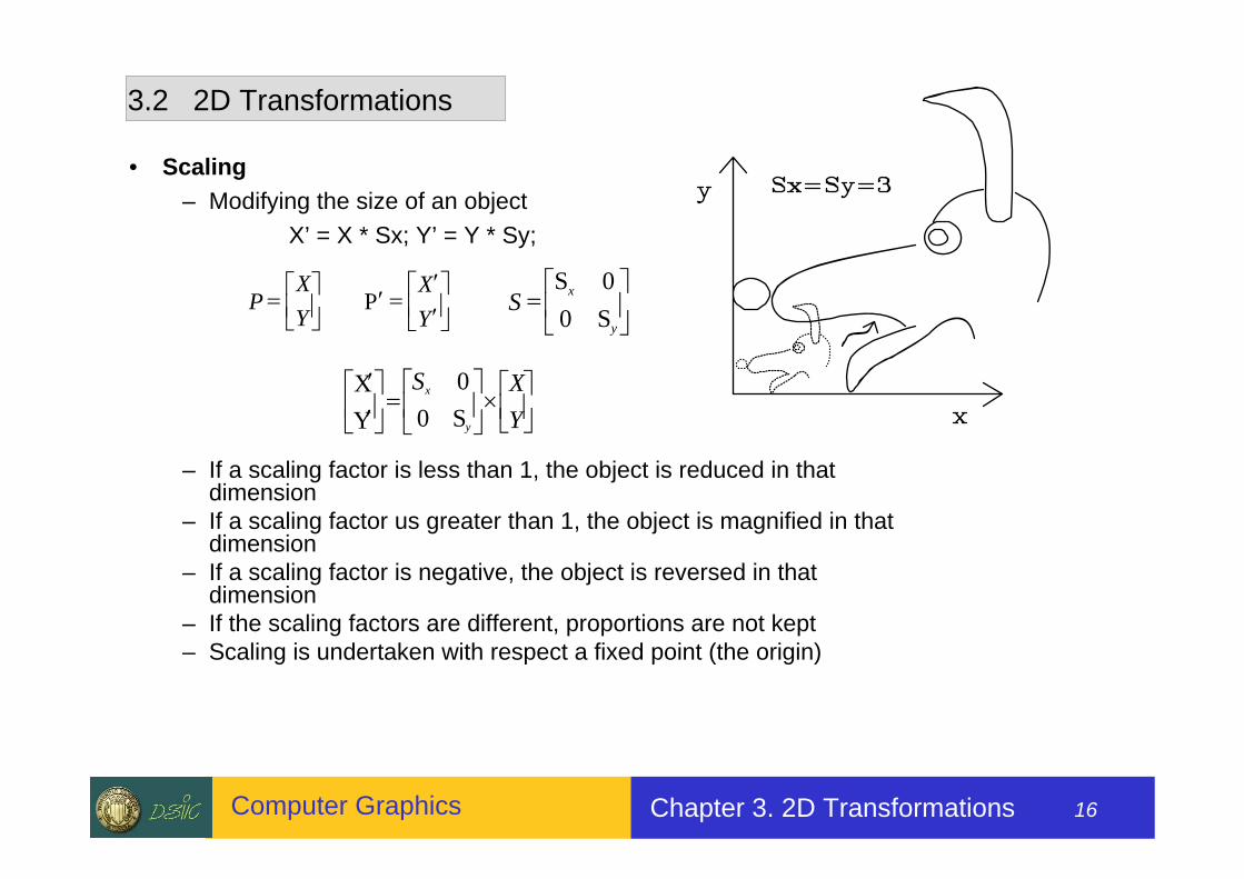
• Scaling– Modifying the size of an object

X’ = X * Sx; Y’ = Y * Sy;

– If a scaling factor is less than 1, the object is reduced in that dimension

– If a scaling factor us greater than 1, the object is magnified in that dimension

– If a scaling factor is negative, the object is reversed in that dimension

– If the scaling factors are different, proportions are not kept– Scaling is undertaken with respect a fixed point (the origin)

SS

Sx

y

=⎡

⎣⎢

⎤

⎦⎥

00

PXY

PXY

= ⎡⎣⎢⎤⎦⎥

′ =′′

⎡

⎣⎢⎤

⎦⎥

′′

⎡

⎣⎢⎤

⎦⎥=⎡

⎣⎢

⎤

⎦⎥×⎡⎣⎢⎤⎦⎥

XY

SS

XY

x

y

00



• Scaling



• Rotation– Rotation of a point with respect another one (in this case the origin)– If a point in polar coordinates (r, β) a rotation is applied:

X’ = r*cos(β+α) = r*(cos(β)*cos(α) - sen(β)*sen (α)) = (r*cos(β))*cos(α) - (r*sen(β))*sen (α) = X*cos(α) - Y*sen (α)

Y’ = r*sen(β+α) = r*(sen(β)*cos(α) + cos(β)*sen (α)) = (r*sen(β))*cos(α) - (r*cos(β))*sen (α) = Y*cos(α) + X*sen (α)

P’ = R * P

( )R =

−⎡

⎣⎢

⎤

⎦⎥

cos sen( )sen( ) cos( )

α αα αr


3.3 Composing transformations

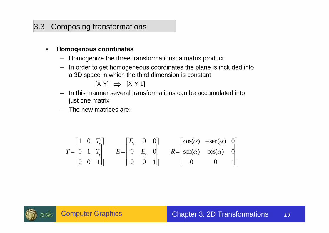
• Homogenous coordinates– Homogenize the three transformations: a matrix product– In order to get homogeneous coordinates the plane is included into

a 3D space in which the third dimension is constant[X Y] [X Y 1]

– In this manner several transformations can be accumulated into just one matrix

– The new matrices are:

⇒

TTT E

EE R

x

y

x

y=⎡

⎣

⎢⎢⎢

⎤

⎦

⎥⎥⎥

=⎡

⎣

⎢⎢⎢

⎤

⎦

⎥⎥⎥

=−⎡

⎣

⎢⎢⎢

⎤

⎦

⎥⎥⎥

1 00 10 0 1

0 00 00 0 1

00

0 0 1

cos( ) sen( )sen( ) cos( )

α αα α



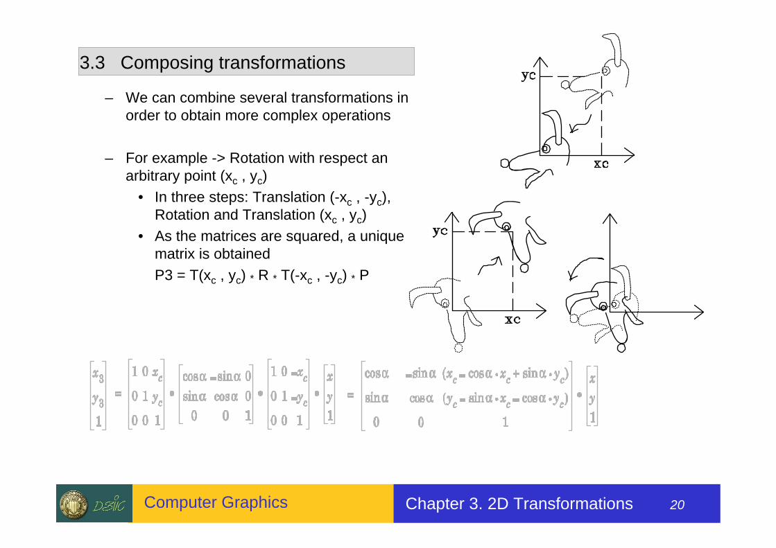
– We can combine several transformations in order to obtain more complex operations

– For example -> Rotation with respect an arbitrary point (xc , yc)

• In three steps: Translation (-xc , -yc), Rotation and Translation (xc , yc)

• As the matrices are squared, a unique matrix is obtainedP3 = T(xc , yc) * R * T(-xc , -yc) * P



• Order of transformations– The matrix product is not commutative

M1*M2<>M2*M1– Transformations either– Transformations that are commutative

• Translation-Translation• Scaling-Scaling• Rotation-Rotation• Proportional scaling-Rotation

– Non-commutative transformations• Translation-Scaling• Traslation-Rotation• Non-proportional scaling-Rotation

Translation after rotation

Rotation after translation


3.4 Geometric transformations around a point

• Complex operations are divided into more simple ones

• Traslation: Translation does not depend on a reference point

• Scaling: Scaling around a reference point (x,y)– Translating the object (-x,-y)– Scaling– Undo translation

• Rotation: Rotations around a center of rotation (CR)– Translating the object(-CR)– Rotation– Undo translation


3.5 Coordinate system transformations

• Real world coordinate system (RWC)– Description of real physic system– Metric units depend on the representation– They have to be converted into device metrics (mapping)– The mapping is composed by a scaling and a shift

• Device coordinate system (DC)– Depends on the device

• Screen size, in pixels• Where the origin is• Positive direction of each coordinate

• Normalized device coordinate system (NDC)– In order to carry out a normalized mapping, a ficticious device of

width and height 1 is used


• How can we go from a coordinate system to another in the most efficient and normalized way

• An area of the real world is defined: window• An area of the device is defined: viewport

– The viewport size goes from a pixel to all the screen– What it is outside the windows goes outside the

viewport• The coordinate transformation from RWC to DC is

carried out into two steps:– From RWC to NCD

• Normalized transformation– From NCD to DC

• Device transformation

Real world coordinates

Normalized coordinate system

windows

viewport



• Window-viewport transformation:– Windows bottom-left corner is moved to origin– Scaling factor are applied in order to force window

an viewport identical sizes– Origin is translated to viewport bottom-left corner

vxmax

vymin

vymax

vxmin

Viewport

wymax

wymin

wxmin wxmax

Window

Real world coordinates

Normalized device coordinates



• NDC to DC is similar to the previous one• In general, windows and viewports are rectangular• Types of transformations between systems:

• Isotropic (keeping proportions, 1 scaling factor) or anisotropic (2 scaling factors). To achieve the isotropic, viewport definition has to be proportional to the window

ISOTROPIC

ANISOTROPIC

Viewport

With clipping

Without clipping

Window


chapter 3users.dsic.upv.es/~jlinares/grafics/chapter 3.pdf · computer graphics tema 3. ... – the...

Documents