Computing covariant Lyapunov vectors, Oseledetsvectors, and dichotomy projectors: a comparative

numerical study

Gary Froyland, Thorsten Huls, Gary Morriss, and Thomas Watson

December 6, 2012

Abstract

Covariant Lyapunov vectors or Oseledets vectors are increasingly being used fora variety of model analyses in areas such as partial differential equations, nonau-tonomous differentiable dynamical systems, and random dynamical systems. Thesevectors identify spatially varying directions of specific asymptotic growth rates andobey equivariance principles. In recent years new computational methods for ap-proximating Oseledets vectors have been developed, motivated by increasing modelcomplexity and greater demands for accuracy. In this numerical study we intro-duce two new approaches based on singular value decomposition and exponentialdichotomies and comparatively review and improve two recent popular approachesof Ginelli et al. [24] and Wolfe and Samelson [43]. We compare the performance ofthe four approaches via three case studies with very different dynamics in terms ofsymmetry, spectral separation, and dimension. We also investigate which methodsperform well with limited data.

1 Introduction

The asymptotic behaviour of a linear ODE x(t) = Ax(t), x(t) ∈ Rd is completely deter-mined by the spectral properties of the d×d matrix A. Similarly, the long-term behaviourof a nonlinear ODE x(t) = f(x(t)) in a small neighbourhood of a fixed point x0, for whichf(x0) = 0, is completely determined by the spectral properties of the linearisation of fat x0. Well-known extensions of these facts can be constructed when x0 is periodic viaFloquet theory. However, for general time-dependent linear ODEs x(t) = A(t)x(t), theeigenvalues of A(t) contain no useful information about the asymptotic behaviour as thesimple example of [8, p. 30] illustrates. On the other hand, if the A(t) are generatedby a process with well-defined statistics, there is a good spectral theory for the systemx(t) = A(t)x(t), and this is the content of the celebrated Oseledets Multiplicative ErgodicTheorem (MET), which we state and explain shortly. The “well-defined statistics” areoften generated by some underlying (typically ergodic) dynamical system.

For clarity of exposition, we will discuss discrete-time dynamics; it is trivial to converta continuous-time system to a discrete-time system by creating eg. time-1 maps flowingfrom time t to time t+1. Let X denote our base space, the space on which the underlying

1

process that controls the time-dependence of the matrices A occurs. As we will place aprobability measure on X, we formally need a σ-algebra X of sets that we can measure1.We denote the underlying process on X by T : X and assume that T is invertible. Oneformally requires that T is measurable2 with respect to X. The “well-defined statistics”are captured by a T -invariant probability measure µ on X; that is, µ = µ ◦ T−1, and wesay that T preserves µ. Finally, it is common to assume that the underlying process isergodic, which means that any subsets X ′ ∈ X of X that are invariant (T−1(X ′) = X ′,implying that trajectories beginning in X ′ stay in X ′ forever in forward and backwardtime) have either µ-measure 0 (they are trivial), or µ-measure 1 (up to sets of µ-measure0 they are all of X).

Now we come to the matrices A, which are generated by a measurable matrix-valuedfunction A : X → Md(R), where Md(R) is the space of d × d real matrices. We choosean initial x ∈ X and begin iterating T to produce an orbit x, Tx, T 2x, . . .. Concurrently,we multiply · · ·A(T 2x) ·A(Tx) ·A(x), and we are interested in the asymptotic behaviourof this matrix product. In particular, we are interested in (i) the growth rates

λ(x, v) := limn→∞

1

nlog ‖A(T n−1x) · · ·A(Tx) · A(x)v‖

as v varies in Rd and (ii) the subspaces W (x) ⊂ Rd on which the various growth ratesoccur. Throughout, ‖·‖ denotes the standard Euclidean vector norm or the associatedmatrix operator norm ‖A‖ = max‖v‖=1 ‖Av‖; whether ‖·‖ is a vector or matrix normwill be clear from the context. Surprisingly, the “well-defined statistics” and ergodicityensures that these limits exist, and that there are at most d different values λ1 > λ2 >· · · > λ` ≥ −∞ that λ(x, v) can take, as v varies over Rd and x varies over µ-almostall of X (note we allow λ` = −∞ to include the case of non-invertible A). We can alsodecompose Rd pointwise in X as Rd =

⊕`i=1 Wi(x), where for all v ∈ Wi(x) \ {0}, one

has

limn→∞

1

nlog ‖A(T n−1x) · · ·A(x)v‖ = λi. (1)

The subspaces Wi are equivariant (or covariant) with respect to A over T ; that is, theysatisfy

Wi(Tx) = A(x)Wi(x) (2)

for 1 ≤ i < `.We use the following stronger version of the MET, which guarantees an Oseledets

splitting even when the matrices A are non-invertible.

Theorem 1.1 ([20], Theorem 4.1). Let T be an invertible ergodic measure-preservingtransformation of the probability space (X,X, µ). Let A : X → Md(R) be a measurablefamily of matrices satisfying ∫

log+ ‖A(x)‖ dµ(x) <∞.

1for example, if X is a topological space, we can set X to be the standard Borel σ-algebra generatedby open sets on X.

2if X is a topological space, and T is continuous, then T is measurable with respect to the standardBorel σ-algebra generated by open sets.

2

Then there exist λ1 > λ2 > · · · > λ` ≥ −∞ and dimensions m1, . . . ,m` with m1 + · · · +m` = d, and a measurable family of subspaces Wi(x) ⊂ Rd such that for µ-almost everyx ∈ X, the following hold.

1. dimWi(x) = mi,

2. Rd =⊕`

i=1Wi(x),

3. A(x)Wi(x) ⊂ Wi(Tx) with equality if λi > −∞,

4. For all v ∈ Wi(x) \ {0}, one has

limn→∞

1

nlog ‖A(T n−1x) · · ·A(x)v‖ = λi.

The range of applications of the MET to the analysis of dynamical systems is vast.Below, we mention just of few of the settings in which the MET is used.

Example 1.2.

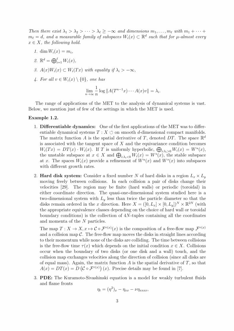
1. Differentiable dynamics: One of the first applications of the MET was to differ-entiable dynamical systems T : X on smooth d-dimensional compact manifolds.The matrix function A is the spatial derivative of T , denoted DT . The space Rd

is associated with the tangent space of X and the equivariance condition becomesWi(Tx) = DT (x) ·Wi(x). If T is uniformly hyperbolic,

⊕i:λi>0Wi(x) = W u(x),

the unstable subspace at x ∈ X and⊕

i:λi<0Wi(x) = W s(x), the stable subspaceat x. The spaces Wi(x) provide a refinement of W u(x) and W s(x) into subspaceswith different growth rates.

2. Hard disk system: Consider a fixed number N of hard disks in a region Lx ×Lymoving freely between collisions. In each collision a pair of disks change theirvelocities [29]. The region may be finite (hard walls) or periodic (toroidal) ineither coordinate direction. The quasi-one-dimensional system studied here is atwo-dimensional system with Ly less than twice the particle diameter so that thedisks remain ordered in the x direction. Here X = ([0, Lx]× [0, Ly])

N × R2N (withthe appropriate equivalence classes depending on the choice of hard wall or toroidalboundary conditions) is the collection of 4N -tuples containing all the coordinatesand momenta of the N particles.

The map T : X → X, x 7→ C ◦ F τ(x)(x) is the composition of a free-flow map F τ(x)

and a collision map C. The free-flow map moves the disks in straight lines accordingto their momentum while none of the disks are colliding. The time between collisionsis the free-flow time τ(x) which depends on the initial condition x ∈ X. Collisionsoccur when the boundary of two disks (or one disk and a wall) touch, and thecollision map exchanges velocities along the direction of collision (since all disks areof equal mass). Again, the matrix function A is the spatial derivative of T , so thatA(x) = DT (x) = D

(C ◦ F τ(x)

)(x). Precise details may be found in [7].

3. PDE: The Kuramoto-Sivashinski equation is a model for weakly turbulent fluidsand flame fronts

ηt = (η2)x − ηxx − νηxxxx,

3

where ν is a damping coefficient. Another familiar example is the complex Ginzburg-Landau equation

ηt = η − (1 + iβ)|η|2η + (1 + iα)ηxx

where η(x, t) is complex and α and β are parameters. In both of these cases it ispossible to approximate solutions of the partial differential equations using Fourierspectral methods (see [11] for details). For instance, in the case of the 1-dimensionalKuramoto-Sivashinski PDE we look for solutions of the form

η(x, t) =∞∑

k=−∞

ak(t)eikx/L,

where L is a unitless length parameter, then solve the following system of ODEsfor the Fourier coefficients ak(t):

ak = (q2k − q4

k)ak − iqk2

∞∑m=−∞

amak−m,

where qk = k/L. Since the ak decrease rapidly with k, truncating the above systemof ODEs is justified.

In the setting of this review we treatX as the space of Fourier coefficients (a1, . . . , ad)of the truncated PDE, and consider the transformation T : X → X defined bychoosing some τ > 0 and letting T ((a1, . . . , ad)) = (a1(τ), . . . , ad(τ)) where theak(t) are solutions to the system of ODEs with initial conditions ak(0) = ak. Thematrix function A is again the spatial derivative of T so that

A(x) = DT (x) =

∂a1(τ)∂a1

∂a1(τ)∂a2

· · ·∂a2(τ)∂a1

∂a2(τ)∂a2

.... . .

.

4. Nonautonomous ODEs and transfer operators: Consider an autonomousODE x(t) = f(x(t)) on X (for example, the Lorenz flow on X = R3), and its flowmap ξ(τ, x) which flows the points x forward τ time units. We think of the coordi-nates x as a “generalised time” and the ODE x(t) = f(x(t)) is our base system. Weuse this base ODE (the driving system) to construct a nonautonomous ODE or skewproduct ODE as y(t) = F (ξ(t, x), y(t)). Given an initial time t and a flow time τ ,

one may construct finite-rank approximations P(τ)x (t) of the Perron-Frobenius op-

erator P(τ)(x(t)) that track the evolution of densities from base “time” x(t) to

x(t+τ); see [22] for details. The matrices P(τ)x (t) form a cocycle and Oseledets sub-

space computations enable the extraction of coherent sets in the nonautonomousflow (see [22]). Coherent sets are time-dependent analogues of almost-invariant setsfor autonomous systems; see [12, 19, 18]. Finite-time constructions for coherentsets are described in [23]. In the setting of this review, T : X → X is defined as

T (x) = ξ(τ, x), and A(x) = P(τ)x (t).

4

From now on, we denote A(T n−1x) · · ·A(x) as A(x, n). The proof of the classicalMET [30] shows that the matrix limit

Ψ(x) = limn→∞

((A(x, n))∗A(x, n))1/2n

(3)

exists for µ-almost all x ∈ X. The matrix Ψ(x) is symmetric, depends measurably on x,and its eigenvalues are eλ1(x) > · · · > eλ`(x). The corresponding eigenspaces are denotedU1(x), . . . , U`(x) and one has

Vi(x) :=⊕j=i

Wj(x) =⊕j=i

Uj(x). (4)

Thus Vi(x) captures growth rates from λi down to λ`; that is, for v ∈ Vi(x) \ Vi+1(x)

λi = limn→∞

1

nlog ‖A(x, n)v‖ . (5)

There are many ways to write the Vi(x) as a direct sum of subspaces Yi(x), . . . , Y`(x)such that (5) holds for v ∈ Yi(x). Two such ways are shown in (4), but one can inductivelychoose the Yi(x) to be any space of dimension mi contained in Vi, with trivial intersectionwith Vi+1(x). Regarding the two possibilities in (5), the “U” decomposition of Vi(x) isorthogonal, while the “W” decomposition (the Oseledets splitting of Theorem 1.1) isequivariant (satisfies property (2)). Thus, Wi(x) is mapped onto Wi(Tx) by A(x), andthe subspaces Wi(x),Wi(Tx),Wi(T

2x), . . ., track the evolution of their elements under thelinear action of A(x), A(Tx), A(T 2x), . . .. On the other hand, the image of Ui(x) underA(x) is in general not mapped onto Ui(Tx) and the same is true of other non-equivariant(or non-covariant) splittings. The splitting given by the Wi(x) is the unique3 splittingwith both the correct growth rates and the equivariance property.

Until recently, classical results provided existence of the splitting Rd = W1(x) ⊕· · · ⊕ W`(x) only in the situation where the matrices A(x), x ∈ X were invertible(see eg. Theorem 3.4.11 [2]), and otherwise, one only obtained a filtration (or flag)Rd = V1(x) ⊃ V2(x) ⊃ · · · ⊃ V`(x) ⊃ V`+1(x) = {0} (see eg. Theorem 3.4.1 [2]).Theorem 1.1 (cf. Theorem 4.1 of [20]) demonstrated that one can remove the invertiblematrix hypothesis and still obtain a splitting; we thus in this paper deal directly with theequivariant splitting Rd = W1(x)⊕ · · ·⊕W`(x) as it separates the vectors into individualsubspaces directly responsible for each distinct Lyapunov exponent, with the additionalimportant dynamical property of equivariance. We call the subspaces of this decompo-sition “Oseledets subspaces”; these are spanned by “Oseledets vectors” (also known as“covariant Lyapunov vectors”4).

3Uniqueness of the Wi(x) is clear in the case where the matrices A(x), x ∈ X are invertible as theWi(x) may be defined to be the spaces with the right growth rates in both forward and backward time(in the backward time case, T−1 and A−1 are used), however the splitting is also unique even when thematrices A are not invertible; see also [21] for an operator setting.

4In the literature, there is an inconsistent use of the term “Lyapunov vector”. In some cases, Lyapunovvectors refer to the subspaces Ui(x), while in others the term refers to the Wi(x). The presence of theadjective “covariant” indicates that one is referring to the equivariant Oseledets vectors Wi(x). Wetherefore use the expressions “Oseledets vector” or “covariant Lyapunov vector” to refer to the Wi(x)and refrain from using “Lyapunov vector”.

5

Non-covariant subspaces such as the Ui(x) have been studied by many authors. Dieciet al. [13, 14, 15] prove convergence rates for SVD and QR methods used to approximatethe Ui(x) above under the assumption of integral separation (discussed later in this sec-tion), as well as convergence rates for approximations of the Sacker-Sell spectrum. Thedirectional information that arises as a byproduct of common QR-based numerical Lya-punov exponent approximation methods [5, 6, 38] has been used extensively to analyseparticle systems [7, 36, 42, 40, 41] and is precisely the above Ui(x) decomposition appliedto the time-reversed system (in the case where both the map T and matrices A(x) areinvertible) [17].

An alternative approach for finding covariant vectors in non-autonomous systems isbased on the so called Sacker-Sell spectrum, cf. [37]. The Sacker-Sell spectrum is definedvia exponential dichotomies, cf. [10, 31] which we briefly introduce for linear differenceequations of the form

wn+1 = Anwn, n ∈ Z, An ∈Md(R) invertible. (6)

In the current context we associate the sequence of matrices {An}n∈Z with an invertiblematrix cocycle over a single orbit, e.g. for some x ∈ X let An = A(T nx). We restrictthe introduction of exponential dichotomies to invertible systems only, and note that ajustification of our algorithm for computing dichotomy projectors strongly depends onthis assumption. Theory defining exponential dichotomies for non-invertible matrices iscontained in eg. [3]. Numerical experiments indicate that Algorithms 3.1 and 3.2 alsoapply in the non-invertible case, however, the corresponding analysis is a topic of futureresearch.

We denote by Φ the solution operator of (6), defined as

Φ(n,m) :=

An−1 . . . Am, for n > m,

I, for n = m,

A−1n . . . A−1

m−1, for n < m.

Definition 1.3. The linear difference equation (6) has an exponential dichotomywith data (K,αs, αu, P

sn, P

un ) on J ⊂ Z, if there exist two families of projectors P s

n andP un = I − P s

n and constants K,αs, αu > 0, such that the following statements hold:

P snΦ(n,m) = Φ(n,m)P s

m ∀n,m ∈ J, (7)

‖Φ(n,m)P sm‖ ≤ Ke−αs(n−m)

‖Φ(m,n)P un ‖ ≤ Ke−αu(n−m)

∀n ≥ m, n,m ∈ J.

Consider the scaled equation

wn+1 = e−λAnwn, n ∈ Z. (8)

Definition 1.4. The Sacker-Sell or dichotomy spectrum is defined as

σED := {λ ∈ R : (8) has no exponential dichotomy on Z}.

The complementary set R \ σED is called the resolvent set.

6

In the literature, the Sacker-Sell spectrum is often defined as the set γ ∈ R+, forwhich the scaled equation

wn+1 =1

γAnwn, n ∈ Z, (9)

has no exponential dichotomy, see, for example [3]. Note that the Sacker-Sell spectrumwith respect to (8) is the logarithm of the Sacker-Sell spectrum with respect to (9).

Under the additional assumptions that An and (An)−1 are uniformly bounded, theSacker-Sell spectrum consists of at most d disjoint, closed intervals, where d denotes thedimension of the space, cf. [37, 4], i.e. there exists an ` < d such that

σED =⋃i=1

[λ−i , λ+i ], where λ+

i+1 < λ−i for i = 1, . . . , `− 1.

It is well known that the Lyapunov spectrum, when it exists, is a subset of the Sacker-Sell spectrum, see [16]. While the Lyapunov spectrum provides information on boundedsolutions of (6) from time 0 to time n ≥ 0, the Sacker-Sell spectrum gives information onbounded solutions from time m to time n. These answers may be different for differentinitial n because, in contrast to the MET setting, there is no a priori stationarity assump-tion on a base dynamical system generating the matrix cocycle. Note that for λ ∈ R \ σED

it follows from [31, Lemma 2.7] that the inhomogeneous equation wn+1 = e−λAnwn + rnhas for every bounded sequence rZ a unique bounded solution on Z.

Dichotomy projectors of the scaled equation (8) are constant in resolvent intervalsRi := (λ+

i , λ−i−1), i = 1, . . . , ` + 1, where λ−0 = ∞ and λ+

`+1 = −∞, see Figure 1. Wedenote these families of projectors by (P i,s

n , P i,un ).

Ri

σED σED

λ−i λ+i λ−i−1 λ+

i−1

Figure 1: Spectral setup.

In analogy to the MET we obtain the family of subspaces

W in = R(P i,s

n ) ∩R(P i+1,un ), n ∈ Z, i = 1, . . . , `

that decompose Rd for each n ∈ Z

Rd =⊕i=1

W in, (10)

and using the invariance property (7) it follows for all i = 1, . . . , ` that

AnWin = W i

n+1, n ∈ Z.

7

Furthermore, for each w ∈ W im, there exists a constant K = K(w) > 0 such that the

following equations hold

‖Φ(n,m)w‖ = Ke(λ+i +r+i (n−m))(n−m), for n ≥ m, where lim sup

n→∞r+i (n) = 0,

‖Φ(n,m)w‖ = Ke(λ−i +r−i (n−m))(n−m), for n < m. where lim sup

n→∞r−i (n) = 0.

Under the assumption of integral separateness one finds d solutions of (6) with pair-wise different exponential growth rates [1, 32]. Consequently, integrally separated systemhave d distinct Lyapunov exponents and these exponents are stable w.r.t. additive pertur-bations of the system, see Theorem 5.4.8 [1]. The latter property is particularly useful forproving error estimates for numerical methods, [13, 14, 15]. In contrast to an integral sep-aration, an exponential separation allows a decomposition into ` < d covariant subspacesRd =

⊕`i=1W

in, such that each pair of solutions from different subspaces, has a different

exponential growth rate; see [33, 9]. Exponential separation and integral separation bothimply a lower bound on the angle between pairs of subspaces with different growth rates;see [9] and references therein. If a discrete time system has an exponential dichotomy,it is exponentially separated, however, the converse is not true, because, for example,exponential separation may be present, but either exponential expansion or contractionmay be absent [9]. In the multiplicative ergodic theorem setting (eg. Theorem 1.1), oneobtains a discrete Lyapunov spectrum with at most d distinct Lyapunov exponents, how-ever without further assumptions, such as exponential separation, in general there is nolower bound on the angle between subspaces in the Oseledets splitting. In the presentwork, we do not assume simplicity of the covariant splitting (10); ie. we do not assumethat dimW i

n = 1 for all i = 1, . . . , d.When working with data over a finite time interval, one has access only to a fi-

nite sequence A0, A1, . . . , An−1. In this case, one either assumes there is an underlyingergodic process generating the sequence A0, A1, . . . , An−1 or one considers exponentialdichotomies.

An outline of the paper is as follows. In Sections 2 and 3, we introduce two newmethods for computing Oseledets vectors. The first method is based on the proof of thegeneralised MET in [20] and is particularly simple to implement and fast to execute.The second method is an adaptation of an approach to compute dichotomy projectors[25]. In Section 4 we review the approaches by Ginelli et al [24] and Wolfe and Samelson[43]. In Sections 2, 3, and 4 we provide MATLAB code snippets to implement thealgorithms presented. Section 5 contains numerical comparisons of the performance ofthe four methods on three dynamical systems. The first case study is a dynamical systemsformed via composition of a sequence of 8× 8 matrices constructed so that all Oseledetsvectors are known at time 0; we thus compare the accuracy of the methods exactly inthis case study. The second case study is an eight-dimensional system generated by twohard disks in a quasi-one-dimensional box. The third case study is a nonlinear modelof time-dependent fluid flow in a cylinder; the matrices are generated by finite-rankapproximations of the corresponding time-dependent transfer operators. The three casestudies have been chosen to represent a cross-section of a variety of features of systemsthat either help or hinder the computation of Oseledets vectors, and we draw out theadvantages and disadvantages of each of the four methods considered.

8

2 An SVD-based approach

The approach outlined in this section is simple to execute and exhibits quick convergence.However, as the length of the sample orbit becomes too large this approach fails.

In [20, proof of Theorem 4.1] it is proven that the limit

limN→∞

A(T−Nx,N)Ui(T−Nx)

exists and is equal to the ith Oseledets subspace Wi(x). That is, if one computes Ui inthe far past and pushes forward to the present, the result is a subspace close to Wi(x).Thus, the strategy in [20] is to first estimate Ui in the past and push forward.

The numerical method of approximating Wj(x), x ∈ X, is implemented in the follow-ing steps:

Algorithm 2.1 (To estimate Wj(x)).

1. Choose M,N > 0 and form the matrix

Ψ(M)(T−Nx) =(A(T−Nx,M)∗A(T−Nx,M)

)1/2M(11)

as an approximation of (3) at T−Nx ∈ X.

2. Compute U(M)j (T−Nx), the jth orthonormal eigenspace of Ψ(M)(T−Nx) as an ap-

proximation of Uj(T−Nx).

3. Define W(M,N)j (x) = A(T−Nx,N)U

(M)j (T−Nx), approximating the Oseledets sub-

space Wj(x).

Listing 1 shows part of a MATLAB implementation of Algorithm 2.1. The arrayA=

[A(T−Nx) | A(T−N+1x) | · · · | A(TM−1x)

]contains the d×d matrices which generate

the cocycle A : X × Z+ → Md(R), and the matrix Psi is formed by multiplying thematrices contained in A. Step 1 of Algorithm 2.1 is performed prior to the code in Listing1, Step 2 is performed in lines 1-3 and lines 4-7 perform Step 3. The function returns Wjas its estimate to Wj(x).

Listing 1: Sample MATLAB code of Algorithm 2.1 to approximate Wj(x)

1 [ ˜ , s , v ] = svd (Psi ) ;2 [ ˜ , p ] = sort (diag (s ) , ’ descend ’ ) ;3 Wj = v ( : , p (j ) )/ norm (v ( : , p (j ) ) ) ;4 for h = 1 : N5 Wj = A ( : , ( h−1)∗dim+1:h∗dim )∗Wj ;6 Wj = Wj/norm (Wj ) ;7 end

The values of M and N can be chosen with relative freedom and in our examples thatfollow we have chosen M = 2N to compute over a time window centred on x, from T−Nx

9

to TNx. Unfortunately, we cannot choose M and N arbitrarily large and expect accurateresults. If A(T−Nx,M) is constructed via the product

A(T−Nx,M) = A(TM−N−1x) · · ·A(T−N+1x)A(T−Nx)

then with larger M the numerical inaccuracies of matrix multiplication compound andthis product becomes more singular and thus a poorer approximation of A(T−Nx,M).Because of this, Ψ(M)(T−Nx) cannot be expected to accurately approximate Ψ(T−Nx) forlarge M . However, even if we suppose Ψ(M)(T−Nx) accurately approximates Ψ(T−Nx),

the small, but non-zero, difference in U(M)j (T−Nx) and Uj(T

−Nx) grows roughly as

O(eN(λ1−λj)

)during the push-forward in step 3 above. For these reasons M and N

must be chosen carefully.

2.1 Improving the basic SVD-based approach

We present a simple improvement that can overcome one of the sources of numericalinstability, namely the push-forward process in step 3 above.

xT−Nkx· · ·T−N1x TMx· · ·

...

Ψ(M)(x)

Ψ(M)(T−Nkx)

Ψ(M)(T−N1x)

...

U(M)j (T−N1x) W

(M,Nk)j (T−Nkx)· · · W

(M,0)j (x)· · ·

Figure 2: Schematic of the re-orthogonalisation described in Section 2.1. The black linerepresents the orbit centred at x ∈ X and the points T−Nkx are those points at whichwe ensure orthogonality with the subspaces Vj(T

−Nkx)⊥. To do this we use the (blue)approximations Ψ(M)(T−Nkx) to approximate Vj(T

−Nkx)⊥ and perform the (red) push-

forward and orthoganlisation steps starting with U(M)j (T−N1x) and ending with W

(M,0)j (x)

(see Algorithm 2.2).

Recall that the subspace Vj(x) = Uj(x) ⊕ · · · ⊕ U`(x) = (U1(x)⊕ · · · ⊕ Uj−1(x))⊥ isA-invariant and that for v ∈ Vj(x)\Vj+1(x) (with V`+1(x) = {0}) we have

λj(x) = limn→∞

1

nlog ‖A(x, n)v‖ .

The subspace Vj(x) contains Wj(x),Wj+1(x), . . . ,W`(x), and so the Oseledets sub-space Wj(x) is necessarily perpendicular to all U1(x), . . . , Uj−1(x). To solve the numericalinstability of step 3 we enforce this condition periodically.

The amended algorithm is implemented as follows:

10

Algorithm 2.2 (To estimate Wj(x)).

1. Choose M,N1 > N2 > · · · > Nn = 0 and form the matrices

Ψ(M)(T−Nkx) =(A(T−Nkx,M)∗A(T−Nkx,M)

)1/2M, k = 1, . . . , n.

2. Compute all the orthonormal eigenspaces U(M)i (T−Nkx), i = 1, . . . , j − 1 of (11)

(replacing N with Nk in (11)) and the eigenspace U(M)j (T−N1x).

3. Let projV : Rd → Rd be the orthogonal projection onto the subspace V so

that ker (projV ) = V ⊥ and V(M)j (x) =

(U

(M)1 (x)⊕ · · · ⊕ U (M)

j−1 (x))⊥

. Define

W(M,N1)j (T−N1x) = U

(M)j (T−N1x), and then define iteratively by pushing forward

and taking orthogonal projections:

W(M,Nk+1)j

(T−Nk+1x

)= proj

V(M)j (T−Nk+1x)

(A(T−Nkx,Nk+1 −Nk

)W

(M,Nk)j

(T−Nkx

))4. W

(M,Nn)j (x) = W

(M,0)j (x) is our approximation of Wj(x).

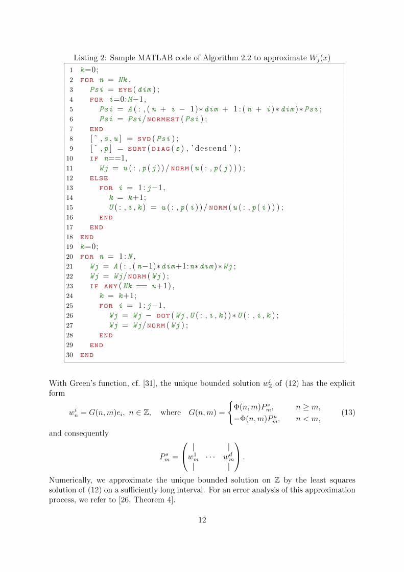
Listing 2 shows an example implementation of Algorithm 2.2 in MATLAB. Lines 1-18 are responsible for performing Steps 1 and 2, whilst the push forward procedure ofStep 3 is performed in lines 20-30. Again, the matrix cocycle is stored in A=

[A(T−Nx)

∣∣A(TN−1x)

∣∣ · · · | A(TM−1x)]

and the function returns Wj as its approximation of Wj(x).The variable Nk is a one-dimensional array containing the elements of {Nk} and is countedby k.

Remark 1. Unfortunately, some numerical issues with this approach remain. They stemprimarily from the long multiplication involved in building the variable Psi of Listings 1and 2. This results in Psi becoming too singular and hence U

(M)j (T−nx) (j 6= 1) poorly

approximates Uj(T−nx). As can be seen in Section 5, Algorithm 2.2 works superbly for

W2(x) as U(M)1 (T−nx) is well approximated for large n. However when estimating Wj(x),

j > 2, a good estimate of U(M)j−1 (x) is required for an accurate projection proj

V(M)j

and for

large n such an estimate becomes unreliable.

3 A dichotomy projector approach

We derive an approach for the computation of a vector wjn ∈ W jn = R(P j,s

n )∩R(P j+1,un ).

For this task, we first need a guess of Λright ∈ Ri and of Λleft ∈ Ri+1 in two neighbouringresolvent intervals that lie close to the common spectral interval, see Figure 3.

Numerical experiments indicate that we get the best results by choosing Λright andΛleft close to (but outside) the second Sacker-Sell interval. This conclusion is supportedby theoretical estimates on the approximation error for Algorithm 3.2, discussed at theend of Section 3.

The following observation from [25, 26] allows the computation of dichotomy projec-tors by solving

win+1 = Anwin + δn,m−1ei, n ∈ Z, ei i-th unit vector. (12)

11

Listing 2: Sample MATLAB code of Algorithm 2.2 to approximate Wj(x)

1 k=0;2 for n = Nk ,3 Psi = eye (dim ) ;4 for i=0:M−1,5 Psi = A ( : , ( n + i − 1)∗dim + 1 : ( n + i )∗dim )∗Psi ;6 Psi = Psi/normest (Psi ) ;7 end

8 [ ˜ , s , u ] = svd (Psi ) ;9 [ ˜ , p ] = sort (diag (s ) , ’ descend ’ ) ;

10 if n==1,11 Wj = u ( : , p (j ) )/ norm (u ( : , p (j ) ) ) ;12 else

13 for i = 1 : j−1,14 k = k+1;15 U ( : , i , k ) = u ( : , p (i ) )/ norm (u ( : , p (i ) ) ) ;16 end

17 end

18 end

19 k=0;20 for n = 1 : N ,21 Wj = A ( : , ( n−1)∗dim+1:n∗dim )∗Wj ;22 Wj = Wj/norm (Wj ) ;23 if any (Nk == n+1) ,24 k = k+1;25 for i = 1 : j−1,26 Wj = Wj − dot (Wj , U ( : , i , k ) )∗U ( : , i , k ) ;27 Wj = Wj/norm (Wj ) ;28 end

29 end

30 end

With Green’s function, cf. [31], the unique bounded solution wiZ of (12) has the explicitform

win = G(n,m)ei, n ∈ Z, where G(n,m) =

{Φ(n,m)P s

m, n ≥ m,

−Φ(n,m)P um, n < m,

(13)

and consequently

P sm =

| |w1m · · · wdm| |

.

Numerically, we approximate the unique bounded solution on Z by the least squaressolution of (12) on a sufficiently long interval. For an error analysis of this approximationprocess, we refer to [26, Theorem 4].

12

Λleft Λright

R3 R2

λ1

Figure 3: Choice of Λleft/right in case i = 2.

The algorithms that we propose in this section compute a vector w ∈ W j0 in analogy

to Wj(x) in the previous sections. For simplicity, we restrict the representation to thecase j = 2 and assume that W 1

n and W 2n are one-dimensional subspaces.

In the absence of information about the dichotomy intervals, one may proceed asfollows. Given a finite sequence of matrices, one can estimate a point in the spectralinterval [λ−q , λ

+q ], q = 1, 2, 3 by computing the (logarithmic) growth rates of one-, two-,

and three-dimensional subspaces using direct multiplication; these growth rates shouldapproximate λ1, λ1+λ2, and λ1+λ2+λ3, respectively. By taking differences to obtain esti-mates λq, q = 1, 2, 3, (the caret indicating estimated quantities) one should obtain values

in the interior of [λ−q , λ+q ], q = 1, 2, 3. We then estimate Λleft = λ2 − (λ2 − λ3)/10 / λ−2

and Λright = λ2 − (λ2 − λ1)/10 ' λ+2 .

In the first step of our first algorithm, we compute a basis of the two-dimensionalspace R(P 3,u

0 ). Then, in the second step, we search for the direction w in this subspacethat additionally lies in R(P 2,s

0 ) and assure in this way that w ∈ R(P 2,s0 )∩R(P 3,u

0 ) = W 20 .

Algorithm 3.1 (A Dichotomy Projector approach to estimate W2(x) by computing W 20 ).

1. Suppose N ∈ N and consider n ∈ [−N,N ] ∩ Z. Let An = A(T nx).

Solve the least squares problem

win+1 = e−Λleft

Anwin + δn,−1r

i, n = −N, . . . , N − 1, i = 1, 2 (14)

such that ‖(wi−N , . . . , wiN)‖2 is minimised,

where the ri are chosen at random and ‖·‖2 is the `2-norm. Define pi := A−1wi−1,

i = 1, 2.

2. Solve for w[0,N ] and κ the least squares problem

wn+1 = e−Λright

Anwn, n = 0, . . . , N − 1, (15)

w0 + κp1 + p2 = 0, (16)

such that ‖(w0, . . . , wN , κ)‖2 is minimised.

Then w0 is our approximation of w2(x) ∈ W2(x).

13

The unique bounded solutions on Z of these two steps satisfy p1, p2 ∈ R(P 3,u0 ) and

these vectors are generically linear independent. Furthermore w0 ∈ R(P 2,s0 ) due to (15)

and w0 ∈ R(P 3,u0 ) due to (16). Thus w0 ∈ R(P 3,u

0 ) ∩R(P 2,s0 ) = W 2

0 .Note that (14) has the form

Bw = r, with B ∈M2dN,d(2N+1)(R), r ∈ R2dN ,

where

B =

−e−Λleft

A−N I. . . . . .

−e−ΛleftAN I

, w =

w−N...

wN−1

,

and the nth entry of r is the vector δn,−1ri ∈ Rd for i = 1, 2.

The least squares solution can be obtained, using the Moore-Penrose inverse:

w = B+r, where B+ = BT (BBT )−1,

cf. [39]. Numerically, we find w by solving the linear system BBTy = r; then w = BTy.Note that in the unlikely case where p1 ∈ W 2

0 , Algorithm 3.1 fails. An alternativeapproach for computing vectors in W 2

0 that avoids this problem is introduced in Algorithm3.2. The main idea of this algorithm is to take a random vector r, project it first toR(P 3,u

0 ) and then eliminate components in the wrong subspaces, by projecting with P 2,s0 .

Algorithm 3.2 (An alternate Dichotomy Projector approach).

1. Again, suppose N ∈ N and consider n ∈ [−N,N ] ∩ Z and let An = A(T nx) asabove. Solve the least squares problem

wn+1 = e−Λleft

Anwn + δn,−1r, n = −N, . . . , N − 1, (17)

such that ‖(w−N , . . . , wN)‖2 is minimised,

where r is chosen at random, and define r′ = A−1w−1.

2. Solve the least squares problem

w′n+1 = e−Λright

Anw′n + δn,−1r

′, n = −N, . . . , N − 1, (18)

such that ‖(w′−N , . . . , w′N)‖2 is minimised.

Then w′0 is our approximation of w2(x) ∈ W2(x).

The solution w0 on Z of these two steps satisfies w0 = P 2,s0 P 3,u

0 r ∈ R(P 2,s0 )∩R(P 3,u

0 ) =W 2

0 .

3.1 Error estimate

We give an error estimate for the solution of Algorithm 3.2 for a finite choice of N . Detailson deriving this estimate are postponed to a forthcoming publication.

For Λleft and Λright close to the boundary of the second Sacker-Sell spectral interval,we denote the dichotomy rates of

wn+1 = e−Λleft

Anwn, wn+1 = e−Λright

Anwn, n ∈ Z (19)

14

Listing 3: Sample MATLAB code for Algorithm 3.1

1 % s t e p 12 B = zeros (2∗N∗dim , 2∗ ( N+1)∗dim ) ;3 for i = 1:2∗N4 B (dim∗(i−1)+1:dim∗i , dim∗(i−1)+1:dim∗i )5 = −exp(−Lambda_left )∗A ( : , dim∗(i−1)+1:dim∗i ) ;6 B (dim∗(i−1)+1:dim∗i , dim∗(i )+1:dim∗(i+1))7 = eye (dim ) ;8 end

9 R = zeros (2∗dim∗N , 2 ) ;10 R (dim∗(N−1)+1:dim∗N , : ) = rand (dim , 2 ) ;11 y = (B∗B ’ ) \ R ;12 u = B ’∗ y ;13 p1 = A ( : , dim∗(N−1)+1:dim∗N )∗u (dim∗(N−1)+1:dim∗N , 1 ) ;14 p2 = A ( : , dim∗(N−1)+1:dim∗N )∗u (dim∗(N−1)+1:dim∗N , 2 ) ;15 p1 = v1/norm (v1 ) ; v2 = v2/norm (v2 ) ;16 % s t e p 217 B = zeros (dim∗(N+1) ,dim∗(N+1)+1);18 for i = 0 : N−119 B (dim∗i+1:dim∗(i+1) ,dim∗i+1:dim∗(i+1))20 = −exp(−Lambda_right )∗A ( : , dim∗(i+N )+1:dim∗(i+N+1)) ;21 B (dim∗i+1:dim∗(i+1) ,dim∗(i+1)+1:dim∗(i+2))22 = eye (dim ) ;23 end

24 B (dim∗N+1:dim∗(N+1) ,1 :dim ) = eye (dim ) ;25 B (dim∗N+1:dim∗(N+1) ,dim∗(N+1)+1) = p1 ;26 R = zeros (dim∗(N+1) ,1) ;27 R (dim∗N+1:dim∗(N+1) ,1) = −p2 ;28 y = (B∗B ’ ) \ R ;29 u = B ’∗ y ;30 w2 = u (dim∗N+1:dim∗(N+1))/norm (u (dim∗N+1:dim∗(N+1))) ;

by (α`,s, α`,u) and (αr,s, αr,u), respectively. Let w0 be the solution of Algorithm 3.2 on Zand let w0 be its approximation for a finite choice of N . Careful estimates show that theapproximation error in the “wrong subspace” R(Q), with Q := I − P 2,s

0 P 3,u0 is given as

‖Q(w0 − w0)‖ ≤ CN(e−α`,sN + e−α

r,uN), (20)

where the constant C > 0 does not depend on N .The exponential dichotomy rates α`,s and αr,u of the difference equations (19) depend

on the choice of Λleft and Λright in the following way: for Λleft in the resolvent set R3 =[λ+

3 , λ−2 ] the difference equation

wn+1 = e−Λleft

Anwn, n ∈ Z

15

Listing 4: Sample MATLAB code for the second step of Algorithm 3.2

1 B = zeros (2∗N∗dim , 2∗ ( N+1)∗dim ) ;2 for i = 1:2∗N3 B (dim∗(i−1)+1:dim∗i , dim∗(i−1)+1:dim∗i )4 = −exp(−Lambda_right )∗A ( : , dim∗(i−1)+1:dim∗i ) ;5 B (dim∗(i−1)+1:dim∗i , dim∗i+1:dim∗(i+1)) = eye (dim ) ;6 end

7 R = zeros (2∗dim∗N , 1 ) ;8 R (dim∗(N−1)+1:dim∗N , : ) = p1 ;9 y = (B∗B ’ ) \ R ;

10 u = B ’∗ y ;11 w2 = u (dim∗N+1:dim∗(N+1))/norm (u (dim∗N+1:dim∗(N+1))) ;

has an exponential dichotomy with stable dichotomy rate α`,s for all α`,s with

0 < α`,s < Λleft − λ+3 .

Similarly, for Λright in the resolvent set R2 = [λ+2 , λ

−1 ] the difference equation

wn+1 = e−Λright

Anwn, n ∈ Z

has an exponential dichotomy with unstable dichotomy rate αr,u for all αr,u with

0 < αr,u < λ−1 − Λright.

Note that both of the above inequalities are strict.Inspecting equation (20), we get the best (smallest) maximal error if we choose Λleft ∈

R3 and Λright ∈ R2 so as to maximise α`,s and αr,u. Consequently, we get the bestnumerical approximations, if Λleft and Λright are chosen close to, but not equal to, theboundary of the common spectral interval [λ−2 , λ

+2 ].

4 The Ginelli and Wolfe schemes

4.1 The Ginelli scheme

The Ginelli Scheme was first presented by Ginelli et al. in [24] as a method for accu-rately computing the covariant Lyapunov vectors of an orbit of an invertible differentiabledynamical system where the A(x) = DT (x) are the Jacobian matrices of the flow or map.

Estimates of the Wj(x) are found by constructing equivariant subspaces Sj(x) =W1(x)⊕· · ·⊕Wj(x) and filtering the invariant directions contained therein using a powermethod on the inverse system restricted to the subspaces Sj(x).

To construct the subspaces Sj(x) we utilise the notion of the stationary Lyapunovbasis [17]. Choose j orthonormal vectors s1(T−nx), s2(T−nx), . . . , sj(T

−nx), n ≥ 1, suchthat si(T

−nx) /∈ Vj+1(T−nx) for 1 ≤ i ≤ j and construct

s(n)i (x) = A(T−nx, n)si(T

−nx), i = 1, . . . , j.

16

Using the Gram-Schmidt procedure, construct the orthonormal basis{s(n)

1 (x), . . . , s(n)j (x)} from {s(n)

1 (x), . . . , s(n)j (x)}, that is,

s(n)1 (x) =

1∥∥∥s(n)1 (x)

∥∥∥ s(n)1 (x),

s(n)2 (x) =

1∥∥∥(s(n)2 (x)−

(s

(n)2 (x) · s(n)

1 (x))s

(n)1 (x)

)∥∥∥(s

(n)2 (x)−

(s

(n)2 (x) · s(n)

1 (x))s

(n)1 (x)

),

(21)

...

Then as n→∞ the basis {s(n)1 (x), . . . , s

(n)j (x)} converges to a set of orthonormal vectors

{s(∞)1 (x), . . . , s

(∞)j (x)} which span the j fastest expanding directions of the cocycle A [17],

that is, if the multiplicities m1 = · · · = mj = 1

Sj(x) := span{s

(∞)1 (x), . . . , s

(∞)j (x)

}= W1(x)⊕ · · · ⊕Wj(x)

= V1(x)\Vj+1(x). (22)

If the Oseledets subspaces are not all one-dimensional, that is the Lyapunov spectrumis degenerate, then we choose Sj(x) only for those j which are the sum of the first kmultiplicities, i.e., j = m1 + · · ·+mk. Then

Sj(x) = W1(x)⊕ · · · ⊕Wk(x)

= V1(x)\Vk+1(x).

In the interest of readability we assume the Oseledets subspaces are one-dimensional butnote that the approach may be extended to the multi-dimensional case.

Note that the Sj(x) are equivariant by construction:

A(x, n)Sj(x) = Sj(Tnx)

provided j ≤ m1 + · · ·+m`−1 if λ` = −∞.We describe the Ginelli approach to finding W2(x). Suppose dimW1(x) =

dimW2(x) = 1 and λ1 > λ2 > −∞ and that the basis {s(∞)1 (x), s

(∞)2 (x)} is known

at x ∈ X. Note first that span{s

(∞)1 (x)

}= W1(x). Let c(x) ∈ R2 denote the coefficients

of w2(x) ∈ W2(x) in the basis {s(∞)1 (x), s

(∞)2 (x)} (recall that the orthogonal projection of

w2(x) onto s(∞)i (x) is zero for i = 3, 4, . . . , d)

then

w2(x) = c1(x)s(∞)1 (x) + c2(x)s

(∞)2 (x).

Lemma 4.1. Let Q(x) denote the d × 2 matrix whose ith column is s(∞)i (x). Then for

each n ≥ 0 there exists an upper triangular, 2× 2 matrix R(x, n) satisfying

A(x, n)Q(x) = Q(T nx)R(x, n). (23)

17

Proof. Note that

A(x, n)Q(x) = A(x, n)

| |s

(∞)1 (x) s

(∞)2 (x)

| |

=

| |A(x, n)s

(∞)1 (x) A(x, n)s

(∞)2 (x)

| |

= Q(T nx)R(x, n)

where

Q(T nx) =

| |s

(∞)1 (T nx) s

(∞)2 (T nx)

| |

and

R(x, n) =

∥∥∥A(x, n)s(∞)1 (x)

∥∥∥ ⟨s

(∞)1 (T nx), A(x, n)s

(∞)2 (x)

⟩0

∥∥∥A(x, n)s(∞)2 (x)

∥∥∥ , (24)

using the equivariance of S1(x) = span{s(∞)1 (x)} and S2(x) = span{s(∞)

1 (x), s(∞)2 (x)}.

Thus, the QR-decomposition of Lemma 4.1 is equivalent to the Gram-Schmidt or-thonormalisation that defines the stationary Lyapunov bases. The columns of Q(T nx)form the stationary Lyapunov basis at T nx.

We have chosen the above notation R(x, n) specifically since, defined in this way, Rforms a cocycle which is the restriction of A to the invariant subspaces Sj.

Lemma 4.2. The matrix R(x, n) defined above forms a cocycle over T .

Proof. Let n,m ≥ 0 then

A(x, n+m)Q(x) = Q(T n+mx)R(x, n+m) (25)

by Lemma 4.1. Since A(x, n+m) = A(T nx,m)A(x, n),

A(x, n+m)Q(x) = A(T nx,m)A(x, n)Q(x)

= A(T nx,m)Q(T nx)R(x, n)

= Q(T n+mx)R(T nx,m)R(x, n). (26)

Equating (25) and (26) gives

R(T nx,m)R(x, n) = R(x, n+m),

as Q(T n+mx) is left-invertible.

18

Since c(x) is the vector of coefficients of the second Oseledets vector of the cocycle A,it is the second Oseledets vector of the cocycle R. To see this, recall w2(x) = Q(x)c(x) ∈W2(x) so that

λ2 = limn→∞

1

nlog ‖A(x, n)Q(x)c(x)‖

which, due to (23), becomes

λ2 = limn→∞

1

nlog ‖Q(T nx)R(x, n)c(x)‖

= limn→∞

1

nlog ‖R(x, n)c(x)‖

since the columns of Q(T nx) are orthonormal.We may approximate c(x) numerically using a simple power method on the inverse

cocycle R−1 (which exists since λ1 > λ2 > −∞).The Ginelli method can be summarised by the following steps:

Algorithm 4.3 (Ginelli method of approximating w2(x) ∈ W2(x)).

1. Choose x ∈ X and M > 0 and form {s(M)1 (x), s

(M)2 (x)} by first randomly se-

lecting two orthonormal vectors {s1(T−Mx), s2(T−Mx)} then performing the push-forward/Gram-Schmidt procedure given by (21). That is, define

s(M)i (x) = A(T−Mx,M)si(T

−Mx), i = 1, 2,

followed by setting

s(M)1 (x) = N

(s

(M)1 (x)

),

s(M)2 (x) = N

(s

(M)2 (x)−

(s

(M)2 (x) · s(M)

1 (x))s

(M)1 (x)

),

where N : v 7→ v/ ‖v‖. The vectors {s(M)1 (x), s

(M)2 (x)} form an approximation to

the stationary Lyapunov basis {s(∞)1 (x), s

(∞)2 (x)}.

2. Choose N > 0 and using the approximate basis {s(M)1 (x), s

(M)2 (x)} in (24), form an

approximation to R(x,N), denoted by R(M)(x,N).

3. Choose c′ ∈ R2 either at random, or by some guess at the second Oseledets vectorof R at TN(x) ∈ X, in this review we found c′ = (0, 1) to work well. Use the inverseiteration method to approximate c(x), that is, define our approximation to c(x) as

c(M,N)(x) = R(M)(x,N)−1c′

= R(M)(TNx,−N)c′

4. Then

w(M,N)2 (x) =

| |s

(M)1 (x) s

(M)2 (x)

| |

c(M,N)(x)

is our approximation to w2(x) ∈ W2(x).

19

As before, there is some freedom of choice of both M and N as well as of the initialorthonormal basis {s1(T−Mx), s2(T−Mx)}, used to approximate S2(x), and of the 2-tuple

c′. The larger M and N are chosen, the more accurate w(M,N)2 (x) will be, provided

s2(T−Mx) /∈ W1(T−Mx)∪V3(T−Mx) and c′ /∈ E1(TMx) where E1 is the Oseledets subspaceof R with Lyapunov exponent λ1.

Listing 5: Sample MATLAB code for Algorithm 4.3

1 [ Q , ˜ ] = qr (rand (dim , j ) , 0 ) ; c = [ zeros (1 ,j−1) 1 ] ;2 for i = 1 : N ,3 QNew = A ( : , ( i−1)∗dim+1:i∗dim )∗Q ;4 [ Q , ˜ ] = qr (QNew , 0 ) ;5 end

6 Q0 = Q ;7 for i = N+1:2∗N+1,8 QNew = A ( : , ( i−1)∗dim +1: i∗dim )∗Q ;9 [ Q , R ] = qr (QNew , 0 ) ;

10 AllR = horzcat (R , AllR ) ;11 end

12 numOfR = size (AllR , 2 ) / j ;13 for i = 1 : numOfR14 R = AllR ( : , ( i−1)∗j+1:i∗j ) ;15 cNew = R\c ;16 c = cNew/norm (cNew ) ;17 end

18 w = Q0∗c ;

Listing 5 shows an example implementation of Algorithm 4.3 in MATLAB whichapproximates wj(x) ∈ Wj(x) using M = N and s1(T−Mx), . . . , sj(T

−Mx) are chosenat random and c′ = ( 0, . . . , 0︸ ︷︷ ︸

j−1 entries

, 1). Lines 2 through 6 construct the approximation of

the stationary Lyapunov basis,{s

(M)1 (x), . . . , s

(M)j (x)

}which is stored as columns of

the matrix Q(x) represented as the variable Q0, while lines 7 through 11 construct thecocycle R stored in AllR as [R(x) | R(Tx) | · · · | R(TNx)]. Lines 12 through 17 performa simple power method on R(x,N)−1 to find the coefficient vector c, which represents the

approximation of wj(x) in the basis{s

(M)1 (x), . . . , s

(M)j (x)

}. Thus, the approximation is

given by Q(x)c. Although Algorithm 4.3 is specific to the case where j = 2, Listing 5 isapplicable to any j for which R(x,N)−1 exists.

It can be shown that, in this case where the top Lyapunov exponent has multiplicity1, E1 = span{(1, 0)T}.

Lemma 4.4. If the first Lyapunov exponent has multiplicity 1, the dominant Oseledetssubspace of the cocycle R is E1 = span{(1, 0)T}.

Proof. Recall that s(∞)1 (x) ∈ W1(x) since span

{s

(∞)1 (x)

}= S1(x) = V1(x)\V2(x) (from

20

(22)) and for all s ∈ V1(x)\V2(x)

λ1 = limn→∞

1

nlog ‖A(x, n)s‖ .

We may write s = Q(x)(a, 0)T for some a ∈ R then

λ1 = limn→∞

1

nlog∥∥A(x, n)Q(x)(a, 0)T

∥∥= lim

n→∞

1

nlog∥∥Q(T nx)R(x, n)(a, 0)T

∥∥and since ‖Q(T nx)s‖ = ‖s‖ (the columns of Q are orthonormal)

λ1 = limn→∞

1

nlog∥∥R(x, n)(a, 0)T

∥∥ .Since S1 is A-invariant, span{(1, 0)T} is R-invariant and the proof is complete.

4.1.1 Limited Data Scenario

In the case where convergence isn’t satisfactory because the amount of cocycle dataavailable is too small (for any M and N to be small), the approximations from Algorithm4.3 can be improved by using better guesses at s1(T−Mx), s2(T−Mx) and c′.

Note that s(∞)1 (x) and s

(∞)2 (x) are two orthonormal vectors optimised for maximal

growth over the time interval [−∞, 0] ∩ Z. In the situation where the values of M andN are limited, one can choose those two vectors that are optimised for growth over theshorter time interval [−M, 0] ∩ Z. In [43] this is achieved by computing the left singularvectors of A(T−Mx,M). This approach works well for small M but can become inaccuratefor very large M for the reasons in Remark 1.

In practice, we have observed that a combination of Step 1 in Algorithm 4.3 and theabove provides the most robust method of accurately approximating s

(∞)1 (x) and s

(∞)2 (x).

As an alternative to Algorithm 4.3 the following may be used: For M ≥ M ′, computevectors optimised for growth from −M to −M + M ′, then push-forward these vectorsfrom −M +M ′ to 0.

Algorithm 4.5 ( Improved Algorithm 4.3).

1. Choose x ∈ X and M ≥ M ′ > 0. Compute the two left singular vectorsof A(T−Mx,M ′) corresponding to the two largest singular values and call them

s1(T−M+M ′x) and s2(T−M+M ′x). Now define{s

(M,M ′)1 (x), s

(M,M ′)2 (x)

}as an ap-

proximation to{s

(∞)1 (x), s

(∞)2 (x)

}by the Gram-Schmidt orthonormalisation of

A(T−M+M ′x,M −M ′)s1(T−M+M ′x) and A(T−M+M ′x,M −M ′)s2(T−M+M ′x) as in(21).

Steps 2–4 as in Algorithm 4.3.

In practice, one should choose M ′ large enough so that enough data is sampled, butnot so large that A(T−Mx,M ′) is too singular.

21

4.2 The Wolfe scheme

The approach followed by Wolfe et al. [43] directly computes the subspace splittingas the intersection of two sets of invariant subspaces. The description of the numericalconstruction of the subspaces Sj(x) featured below differs slightly from [43], however,the essential features of the approach are retained. In fact, the constructions featuredhere improve upon those in [43] in terms of accuracy versus amount of cocycle data used

– in the notation of Algorithm 4.6 below, if M1 is made larger, w(M1,M ′1,M2)2 (x) is more

accurate, which is not the case in [43] for the same reasons discussed in Remark 1.Recall the eigenspace decomposition Uj(x) of the limiting matrix Ψ(x) presented in

Section 2 and define Vj(x) = Uj(x) ⊕ · · · ⊕ U`(x). Recall that Vj(x) ⊃ Wj(x),Wj+1(x),. . . ,W`(x). Also recall from the previous section that Sj(x) ⊃ W1(x),W2(x), . . . ,Wj(x).Thus

Wj(x) = Vj(x) ∩ Sj(x).

Again, in the interest of readability we assume the Oseledets subspaces Wj(x), andthe eigenspaces Uj(x), are one-dimensional. As in the case of the previous section, theideas here may be extended to the case in which the Oseledets subspaces are not one-dimensional. Let uj(x) be the singular vector spanning Uj(x) and let sj(x) = s

(∞)j (x) be

the jth element of the stationary Lyapunov basis as in the previous section. Then note

wj(x) =

j∑i=1

〈wj(x), si(x)〉 si(x),

wj(x) =d∑i=j

〈wj(x), ui(x)〉ui(x).

Taking inner products with uk(x) and sk(x) respectively gives

〈wj(x), uk(x)〉 =

j∑i=1

〈wj(x), si(x)〉 〈si(x), uk(x)〉 for k ≥ j, (27)

〈wj(x), sk(x)〉 =d∑i=j

〈wj(x), ui(x)〉 〈ui(x), sk(x)〉 for k ≤ j. (28)

Substituting (27) into (28) and rearranging gives

〈wj(x), sk(x)〉 =

j∑i=1

(d∑h=j

〈sk(x), uh(x)〉 〈uh(x), si(x)〉

)〈si(x), wj(x)〉 . (29)

Note that∑d

h=1 〈sk(x), uh(x)〉 〈uh(x), si(x)〉 = δki so

d∑h=j

〈sk(x), uh(x)〉 〈uh(x), si(x)〉 = δki −j−1∑h=1

〈sk(x), uh(x)〉 〈uh(x), si(x)〉 .

22

Then (29) becomes

〈wj(x), sk(x)〉 =

j∑i=1

δki 〈si(x), wj(x)〉 −j∑i=1

j−1∑h=1

〈sk(x), uh(x)〉 〈uh(x), si(x)〉 〈si(x), wj(x)〉

= 〈sk(x), wj(x)〉 −j∑i=1

j−1∑h=1

〈sk(x), uh(x)〉 〈uh(x), si(x)〉 〈si(x), wj(x)〉

0 =

j∑i=1

j−1∑h=1

〈sk(x), uh(x)〉 〈uh(x), si(x)〉 〈si(x), wj(x)〉 . (30)

Equation (30) may be considered as a j × j homogeneous linear equation by defining amatrix entry-wise as

Dki =

j−1∑h=1

〈sk(x), uh(x)〉 〈uh(x), si(x)〉

and solving

Dy = 0,

where yi = 〈si(x), wj(x)〉. The entries of y are then the coefficients of wj(x) with respectto the basis s1(x) . . . , sj(x).

The Wolfe approach may be implemented as follows:

Algorithm 4.6 (Improved Wolfe approach to approximating wj(x) ∈ Wj(x)).

1. Choose x ∈ X and M1 ≥ M ′1 > 0 and construct {s(M1,M ′1)

1 (x), . . . , s(M1,M ′1)j (x)} as

an approximation of the stationary Lyapunov basis vectors {s(∞)1 (x), . . . , s

(∞)j (x)}

using the methods outlined in Step 1 of Algorithm 4.5, that is, compute the leftsingular vectors of A(T−M1x,M ′

1) corresponding to the j− 1 largest singular values

and call them si(T−M1+M ′1x), i = 1, . . . , j − 1. Then form the s

(M1,M ′1)i (x) by the

Gram-Schmidt orthornormalisation of A(T−M1+M ′1x,M1−M ′1)si(T

−M1+M ′1x) for i =1, . . . , j − 1.

2. Choose M2 > 0 and construct the one-dimensional eigenspaces U(M2)1 (x), . . . ,

U(M2)j−1 (x) as approximations to the eigenspaces U1(x), . . . , Uj−1(x) as in Step 1 of

Algorithm 2.1, that is, construct

Ψ(M2)(x) = (A(x,M2)∗A(x,M2))1/2M2 ,

and let U(M2)i (x) be the ith orthonormal eigenspace of Ψ(M2)(x). Define u

(M2)i (x) ∈

U(M2)i (x), i = 1, . . . , j − 1.

3. Form the matrix D as above:

Dki =

j−1∑h=1

⟨s

(M1,M ′1)k (x), u

(M2)h (x)

⟩⟨u

(M2)h (x), s

(M1,M ′1)i (x)

⟩.

23

4. Solve the homogeneous linear equation Dy = 0. Then w(M1,M ′1,M2)j =

∑ji=1 yisi(x)

forms our approximation of wj(x) ∈ Wj(x).

This approach suffers from the same numerical stability issue of Algorithm 2.2 of Sec-tion 2.1. Namely, the vector spaces U

(M)1 (x), . . . , U

(M)j−1 (x) may only poorly approximate

U1(x), . . . , Uj−1(x) for M too large (see the final paragraph of Section 2.1).A recent paper [27] provides alternative descriptions of both the Ginelli et al. and

Wolfe and Samelson methods, well-suited to those familiar with the QR-decompositionbased numerical method for estimating Lyapunov exponents due to Benettin et al. [5, 6]and Shimada and Nagashima [38]. The discussion in [27] is restricted to invertible cocyclesgenerated by the Jacobian matrices of a dynamical system. Although this assumptionallows stable numerical methods to be constructed, i.e., better convergence obtained forlarger data sets, it means some important examples in which the matrix cocycle is non-invertible are overlooked, for example the case study of Section 5.3. While the memoryfootprint of the implementations discussed in [27] is estimated, there is no discussionof convergence rates or accuracy with respect to the amount of cocycle data available.Finally, while the examples featured in [27] explain the methods presented in the contextof differentiable dynamical systems the case studies of Section 5 in the present paperfocus on comparative performance of the methods presented, via a broad range of possibleapplications.

5 Numerical comparisons of the four approaches

We present three detailed case studies, comparing the four approaches for calculatingOseledets subspaces. The first case study is a nontrivial model for which we know theOseledets subspaces exactly and can therefore precisely measure the accuracy of themethods. The second case study produces a relatively low-dimensional matrix cocycle,while the third case study generates a very high-dimensional matrix cocycle; in these casestudies we use two fundamental properties of Oseledets subspaces to assess the accuracyof the four approaches.

5.1 Case Study 1: An exact model

In general the Oseledets subspaces cannot be found analytically which makes the task ofdetermining the efficacy of the above approaches difficult. However, the exact model de-scribed below allows us to compare the numerical approximations with the exact solutionby building a cocycle in which the subspaces are known a priori.

We generate a system with simple Lyapunov spectrum λ1 > λ2 > · · · > λd > −∞.We form a diagonal matrix

R =

eλ1 0

eλ2

. . .

0 eλd

24

and generate the cocycle by the sequence of matrices {An} where

An = SnRS−1n−1

Sn =

I + εZ, for n 6= −1, n ∈ [−N,N ] ∩ Z,

I +

0

z2 0. . . . . .

zd 0

, for n = −1.(31)

The entries of Z and the numbers z2, . . . , zd are uniformly randomly generated from theinterval [0, 1]. By construction, the columns of Sn−1 span the Oseledets subspaces at timen ∈ [−N,N ] ∩ Z.

We compare the exact result at time n = 0 with the approximations computed bythe various algorithms for d = 8, {λ1, . . . , λ8} = {log 8, log 7, log 6, . . . , log 1} and ε = 0.1for varying amounts of cocycle data

{A(T−Nx), . . . , A(TNx)

}. The exact model has a

well separated spectrum, is generated using invertible matrices, and is of relatively lowdimension.

For this model we use the following choice of parameters to execute the algorithms:

• Algorithm 2.2: M = N and {Nk} = {1, 6, . . . , 5k − 4, . . . , 5K − 4, N} where5K − 4 < N ≤ 5K + 1.

• Algorithm 3.1: We estimate the three largest Lyapunov exponents λ1 > λ2 > λ3

and set Λright = λ2 + 0.1(λ1 − λ2) and Λleft = λ2 − 0.1(λ2 − λ3).

• Algorithm 3.2: As for Algorithm 3.1.

• Algorithm 4.5: M = N , M ′ = 5, and c′ = (0, 1).

• Algorithm 4.6: Let M1 = N , M ′1 = 5 and M2 = N .

Figure 4 compares the approximations yielded from the various approaches outlinedin Sections 2, 3 and 4 with the known solution of Equation (31). Each algorithm exhibitsapproximately exponential convergence with respect to the length of the sample cocycleup to (almost) machine accuracy of about 10−16. Algorithm 4.3 is notably erratic whereasthe other algorithms converge smoothly, which suggests that in the limited data scenario(small N) it represents the less satisfactory choice.

Performing a linear regression on the data shown in Figure 4 for a sample whereeach method is still converging (N . 230) yields a gradient of −0.13342 ≈ log 7 − log 8suggesting that the convergence rate is roughly exponential in the difference of the largestand 2nd largest Lyapunov exponent.

Algorithm 2.2 is slightly more accurate than the other algorithms for large N , whilethere is a limit to the accuracy of Algorithms 3.1 and 3.2.

It is worth noting that Algorithms 2.2 and 4.6 do not perform as well when approxi-mating Oseledets subspaces corresponding to Lyapunov exponents λ3, . . . , λ`. Whilst theyreach machine accuracy with ease for W1 and W2, forming A(x, n) = A(T n−1x) · · ·A(x)via numerical matrix multiplication produces greater inaccuracies for subspaces W3

25

0 50 100 150 200 250 300 35010−18

10−16

10−14

10−12

10−10

10−8

10−6

10−4

10−2

100

102

N

∥ ∥ ∥w(N)

2(x

)−w

2(x

)∥ ∥ ∥Algorithm 2.2Algorithm 3.1Algorithm 3.2Algorithm 4.5Algorithm 4.6

Figure 4: Comparing the approximations of the second Oseledets subspace W(N)2 (x)

with the exact solution W2(x) which is known a priori. Each “N -approximation” iscomputed using cocycle data {A(T−Nx), A(T−N+1x), . . . , A(TNx)}. The comparison is

simply the Euclidean norm of the separation of the two unit vectors w(N)2 (x) ∈ W (N)

2 (x)and w2(x) ∈ W2(x).

through W` (see Remark 1). On the other hand, Algorithms 3.1, 3.2 and 4.5 do notsuffer from the same issue because they do not need to form A(x, n) but use only thegenerating matrices A(x). As such, they still reach machine accuracy, although a greateramount of data (larger N) is required.

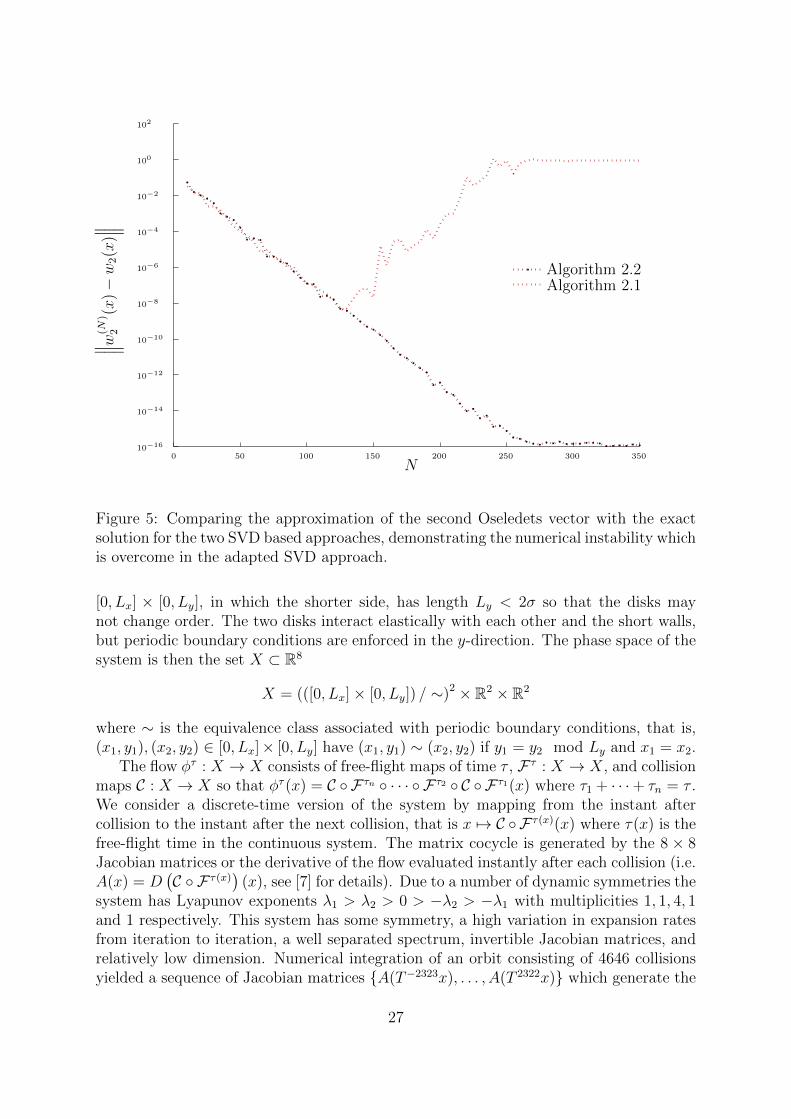
Figure 5 is similar to Figure 4 except that it compares only Algorithms 2.1 and 2.2.In doing so, it highlights the result of one of the numerical instabilities of Algorithm 2.1,namely the pushing forward of U

(M)j (T−Nx) in Step 3.

Finally, Figure 6 shows the execution times of Algorithms 2.2, 3.1, 3.2, 4.5 and 4.6,which were timed using MATLAB’s timing functionality. The most time-consuming stepin Algorithm 4.5 is the SVD performed as part of the alterations from Section 4.1.1.Algorithm 4.6 must perform two SVDs and Algorithm 2.2 must perform many more,which accounts for their longer execution times.

5.2 Case Study 2: Particle dynamics - two disks in a quasi-one-dimensional box

We consider the quasi-one-dimensional heat system studied extensively by Morriss et al.[7, 29, 36, 42, 40, 41] which consists of two disks of diameter σ = 1 in a rectangular box,

26

0 50 100 150 200 250 300 35010−16

10−14

10−12

10−10

10−8

10−6

10−4

10−2

100

102

N

∥ ∥ ∥w(N)

2(x

)−w

2(x

)∥ ∥ ∥

Algorithm 2.2Algorithm 2.1

Figure 5: Comparing the approximation of the second Oseledets vector with the exactsolution for the two SVD based approaches, demonstrating the numerical instability whichis overcome in the adapted SVD approach.

[0, Lx] × [0, Ly], in which the shorter side, has length Ly < 2σ so that the disks maynot change order. The two disks interact elastically with each other and the short walls,but periodic boundary conditions are enforced in the y-direction. The phase space of thesystem is then the set X ⊂ R8

X = (([0, Lx]× [0, Ly]) / ∼)2 × R2 × R2

where ∼ is the equivalence class associated with periodic boundary conditions, that is,(x1, y1), (x2, y2) ∈ [0, Lx]× [0, Ly] have (x1, y1) ∼ (x2, y2) if y1 = y2 mod Ly and x1 = x2.

The flow φτ : X → X consists of free-flight maps of time τ , F τ : X → X, and collisionmaps C : X → X so that φτ (x) = C ◦ F τn ◦ · · · ◦ F τ2 ◦ C ◦ F τ1(x) where τ1 + · · ·+ τn = τ .We consider a discrete-time version of the system by mapping from the instant aftercollision to the instant after the next collision, that is x 7→ C ◦F τ(x)(x) where τ(x) is thefree-flight time in the continuous system. The matrix cocycle is generated by the 8 × 8Jacobian matrices or the derivative of the flow evaluated instantly after each collision (i.e.A(x) = D

(C ◦ F τ(x)

)(x), see [7] for details). Due to a number of dynamic symmetries the

system has Lyapunov exponents λ1 > λ2 > 0 > −λ2 > −λ1 with multiplicities 1, 1, 4, 1and 1 respectively. This system has some symmetry, a high variation in expansion ratesfrom iteration to iteration, a well separated spectrum, invertible Jacobian matrices, andrelatively low dimension. Numerical integration of an orbit consisting of 4646 collisionsyielded a sequence of Jacobian matrices {A(T−2323x), . . . , A(T 2322x)} which generate the

27

0 50 100 150 200 250 300 35010−4

10−3

10−2

10−1

100

101

Algorithm 2.2Algorithm 3.1Algorithm 3.2Algorithm 4.5Algorithm 4.6

N

τ

Figure 6: Comparing the execution time τ of the various algorithms using MAT-LAB’s timing functionality. Each algorithm is executed using the cocycle data{A(T−Nx), . . . , A(TNx)

}.

cocycle A.For this model we use the same choice of parameters to execute the algorithms as

with the previous model:

• Algorithm 2.2: M = N and {Nk} = {1, 6, . . . , 5k − 4, . . . , 5K − 4, N} where5K − 4 < N ≤ 5K + 1.

• Algorithm 3.1: We estimate the three largest Lyapunov exponents λ1 > λ2 > λ3

and set Λright = λ2 + 0.1(λ1 − λ2) and Λleft = λ2 − 0.1(λ2 − λ3).

• Algorithm 3.2: As for Algorithm 3.1.

• Algorithm 4.5: M = N , M ′ = 5, and c′ = (0, 1).

• Algorithm 4.6: Let M1 = N , M ′1 = 5 and M2 = N .

5.2.1 Criteria to assess the accuracy of estimated Oseledets spaces

Since the Oseledets subspaces for this model are unknown, we test the approximationsfor two properties of Oseledets subspaces, namely their equivariance and the expansionrate, which defines the corresponding Lyapunov exponent.

28

Equivariance: To test for equivariance, we approximate the second Oseledetsvector, w

(N)2 (T nx), at each time n = 0, 1, . . . , 30. We then compute∥∥∥N (A(x, n)w

(N)2 (x)

)− w(N)

2 (T nx)∥∥∥ and plot the result, where v

N7→v/ ‖v‖. If the ap-

proximations are equivariant this value would be zero.

Expansion Rate: To test the expansion rate, each approach is used to computethe second Oseledets vector, w

(N)2 (x) ∈ W

(N)2 (x), at time n = 0 and we plot

1m

log∥∥∥A(x,m)w

(N)2 (x)

∥∥∥ versus m. If W(N)2 (x) is accurate, elements of W

(N)2 (x) should

grow at the correct rate: λ2.Whilst the Oseledets vector w2(x) must satisfy the above two properties, we must be

careful when examining the results of these numerical experiments. For instance, (i) it ispossible to choose vectors that are equivariant despite not being contained in any singleOseledets subspace, and (ii) any element of V2(x)\V3(x) ! W2(x) (a much larger set thanW2(x)) has Lyapunov exponent λ2.

5.2.2 Numerical Results

Figure 7 shows the results of the equivariance test for the quasi-one-dimensional two diskmodel. At the lower end of cocycle data length (N = 75) all Algorithms except 3.2display reasonable equivariance, although Algorithm 3.1 remains equivariant for only ahandful of steps. For N = 150 and N = 225 all approaches appear to produce close toequivariant results (note the changing scales in the vertical direction), with Algorithms3.1 and 3.2 lagging behind when N = 225.

Figure 8 shows the results of the expansion rate test for the quasi-one-dimensional twodisk model for various amounts of cocycle data

{A(T−Nx), . . . , A(TNx)

}. As expected,

when there is a limited amount of data available (N small) the approximations eitherexpand at the higher rate of λ1 or only expand at the rate of λ2 for a brief time beforethe error grows too large. As N is increased, the approximations expand at λ2 for longerperiods, suggesting that they more accurately represent w2(x).

Most algorithms perform similarly regarding expansion rate. Note that the amountof cocycle data (size of N) needed to perform well in the Expansion Rate test is less thanthat needed to perform well in the Equivariance test - this demonstrates the importanceof good performance in both tests in order to assess whether or not the algorithms areperforming well.

5.3 Case Study 3: Time-dependent fluid flow in a cylinder; atransfer operator description

An important emerging application for Oseledets subspaces is the detection of strangeeigenmodes, persistent patterns, and coherent sets for aperiodic time-dependent fluidflows. In the periodic setting strange eigenmodes have been found as eigenfunctions ofa Perron-Frobenius operator via classical Floquet theory; [34, 28, 35]. However, in theaperiodic time-dependent setting, Floquet theory cannot be applied. An extension toaperiodically driven flows was derived in [22], based on the new multiplicative ergodictheory of [20]. Discrete approximations of a Perron-Frobenius cocycle representing the

29

Algorithm 2.2Algorithm 3.1Algorithm 3.2Algorithm 4.5Algoirthm 4.6

m

∥ ∥ ∥N( A(x,m

)w(N

)2

(x)) −

w(N

)2

(Tm

(x))∥ ∥ ∥

m

∥ ∥ ∥N( A(x,m

)w(N

)2

(x)) −

w(N

)2

(Tm

(x))∥ ∥ ∥

m

∥ ∥ ∥N( A(x,m

)w(N

)2

(x)) −

w(N

)2

(Tm

(x))∥ ∥ ∥

0 5 10 15 20 25 3010−6

10−5

10−4

10−3

10−2

10−1

100

101

0 5 10 15 20 25 3010−12

10−11

10−10

10−9

10−8

10−7

10−6

10−5

10−4

0 5 10 15 20 25 3010−14

10−13

10−12

10−11

10−10

10−9

10−8

10−7

10−6

10−5

Figure 7: The equivariance test for the various algorithms on the quasi-one-dimensionaltwo disk model. Each approach is used to approximate the second Oseledets vector,w

(N)2 (T nx) ∈ W (N)

2 (T nx) using cocycle data {A(T−Nx), . . . , A(TNx)}, at each time n =

0, 1, . . . , 30. We then compute∥∥∥NA(x, n)w

(N)2 (x)− w(N)

2 (T nx)∥∥∥ and plot the result. Note

the different scales on each vertical axis. The plots shown are for N = 75 (top left),N = 150 (top right) and N = 225 (bottom).

aperiodic flow are constructed and in this aperiodic setting the leading sub-dominant Os-eledets subspaces play the role of the leading sub-dominant eigenfunctions in the periodicforcing case.

We review the four methods of approximating Oseledets subspaces with the aperiod-ically driven cylinder flow from [22]. The flow domain is Y = [0, 2π]× [0, π], t ∈ R+ andthe flow is defined by the following forced ODE:

x = c− A(z(t)) sin(x− νz(t)) cos(y) + εG(g(x, y, z(t))) sin(z(t)/2) mod 2π

y = A(z(t)) cos(x− νz(t)) sin(y).(32)

Here, z(t) = 6.6685z1(t), where z1(t) is generated by the standard Lorenz flow,A(z(t)) = 1 + 0.125 sin(

√5z(t)), G(ψ) := 1/(ψ2 + 1)

2and the parameter function

30

Algorithm 2.2Algorithm 3.1Algorithm 3.2Algorithm 4.5Algorithm 4.6

m

1 mlo

g∥ ∥ ∥A(x

,m)w

(N)

2(x

)∥ ∥ ∥

m

1 mlo

g∥ ∥ ∥A(x

,m)w

(N)

2(x

)∥ ∥ ∥

m

1 mlo

g∥ ∥ ∥A(x

,m)w

(N)

2(x

)∥ ∥ ∥

0 20 40 60 80 100 120 140 160 180 2000.18

0.2

0.22

0.24

0.26

0.28

0.3

0.32

0.34

0 20 40 60 80 100 120 140 160 180 200

0.16

0.18

0.2

0.22

0.24

0.26

0.28

0.3

0.32

0.34

0 20 40 60 80 100 120 140 160 180 2000.18

0.2

0.22

0.24

0.26

0.28

0.3

0.32

0.34

Figure 8: The expansion rate test for the various approaches on the quasi-one-dimensionaltwo disk model. The second Oseledets vector, w

(N)2 (x) ∈ W (N)

2 (x), is approximated using

cocycle data {A(T−Nx), . . . , A(TNx)} and we plot 1m

log∥∥∥A(x,m)w

(N)2 (x)

∥∥∥ versus m. If

the approximation is accurate this quantity should tend to the value of λ2 ≈ 0.210,otherwise it would tend to the value of λ1 ≈ 0.325 both of which are shown in blue. Theplots shown are for N = 25 (top left), N = 75 (top right) and N = 150 (bottom).

ψ = g(x, y, z(t)) := sin(x−νz(t)) sin(y)+y/2−π/4 vanishes at the level set of the stream-function of the unperturbed (ε = 0) flow at instantaneous time t = 0, i.e., s(x, y, 0) = π/4,which divides the phase space in half.

We set ε = 1 as this value is sufficiently large to ensure no KAM tori remain in thejet regime, but sufficiently small to maintain islands originating from the nested periodicorbits around the elliptic points of the unperturbed system.

We construct the discretised Perron-Frobenius matrices P(τ)x (t) =: A(x) as described

in Section 3 of [22], and briefly recapped in Example 1.2, using a uniform grid of 120×60boxes, τ = 8 and −32 ≤ t ≤ 32. In total, we generate 8 such matrices of dimension7200 × 7200. Thus, in this case study we have a limited amount of data, no symmetry,high dimension, and the matrices are non-invertible and sparse.

In order to obtain reasonable results we executed Algorithms 2.2, 3.1, 3.2, 4.3 and 4.6with the following parameters:

• Algorithm 2.2: M = N = 4 and {Nk} = {2, 4}.

31

0 2 4 60

1

2

3

(a)

−0.1

−0.05

0

0.05

0.1

0 2 4 60

1

2

3

(b)

−0.1

−0.05

0

0.05

0.1

0 2 4 60

1

2

3

(c)

0

0.01

0.02

0.03

0.04

0 2 4 60

1

2

3

(d)

−0.1

−0.05

0

0.05

0.1

0 2 4 60

1

2

3

(e)

−0.1

−0.05

0

0.05

0.1

Figure 9: The second Oseledets subspace as determined by (a) Algorithm 2.2, (b) Algo-rithm 3.1, (c) Algorithm 3.2, (d) Algorithm 4.3 and (e) Algorithm 4.6.

• Algorithm 3.1: We estimate the three largest Lyapunov exponents λ1 > λ2 > λ3

and set Λright = λ2 + 0.1(λ1 − λ2) and Λleft = λ2 − 0.1(λ2 − λ3).

• Algorithm 3.2: As for Algorithm 3.1.

• Algorithm 4.5: M ′ = M = 4 (so that only an SVD is used, and no push-forwardstep), N = 4 and c′ = (0, 1).

• Algorithm 4.6: M1 = M ′1 = 4 and M2 = 4.

The results of these numerical experiments are shown in Figures 9 and 10. Recall thatin this setting, the cocycle A(x, n) is a cocycle of discretised Perron-Frobenius operatorsacting on piecewise constant functions defined on Y ; we identify these piecewise constantfunctions (with 7200 pieces) with vectors in R7200. Figure 9 first shows the approximationsof the second Oseledets vector w2(x) at time t = 0. In this setting the Oseledets vectorslocate coherent structures : Figure 10 compares the push-forward of the approximations inFigure 9 with independently computed approximations of w2(Tx) - the second Oseledetsvector at time t = 8.

32

0 2 4 60

1

2

3

(1a)

−0.1

−0.05

0

0.05

0.1

0 2 4 60

1

2

3

(1b)

−0.2

−0.1

0

0.1

0.2

0 2 4 60

1

2

3

(2a)

−0.1

0

0.1

0 2 4 60

1

2

3

(2b)

−0.05

0

0.05

0 2 4 60

1

2

3

(3a)0

0.02

0.04

0.06

0 2 4 60

1

2

3

(3b)

0

0.05

0.1

0 2 4 60

1

2

3

(4a)

−0.1

−0.05

0

0.05

0.1

0 2 4 60

1

2

3

(4b)

−0.2

−0.1

0

0.1

0.2

0 2 4 60

1

2

3

(5a)

−0.1

−0.05

0

0.05

0.1

0 2 4 60

1

2

3

(5b)

−0.2

−0.1

0

0.1

0.2

Figure 10: Comparing the approximations of the second Oseledets vector w2(Tx) at timet = 8 with the push-forward of the approximations at time t = 0. Those labelled (a) are

the push-forwards A(x, 1)w(4)2 (x) whilst those labelled (b) are independently computed

approximations w(4)2 (Tx) of w2(Tx). The algorithms used are as follows: (1) Algorithm

2.2, (2) Algorithm 3.1, (3) Algorithm 3.2, (4) Algorithm 4.3 and (5) Algorithm 4.6.

In this study the data sample is insufficiently long for Algorithm 3.2 to work effectively,but the other algorithms produce similar results. A visual inspection of Figure 10 showsthat the highlighted structures are approximately equivariant/coherent.

6 Conclusion

We introduced two new methods for computing Oseledets subspaces: one based on singu-lar value decompositions and the other based on dichotomy projectors. We also reviewedrecent methods by Ginelli et al. [24] and Wolfe and Samelson [43], and presented an im-provement to both of these approaches that intelligently selected initial bases when onlyshort time series were available to compute with. Finally, we carried out a comparativenumerical investigation involving all four methods.

Generally speaking, we found that Algorithms 2.2, 4.5, and 4.6 outperformed thedichotomy projector methods (Algorithms 3.1 and 3.2) when limited to moderate amountsof data were available, however, the dichotomy projector methods performed very wellwhen long time series of matrices were available. The Ginelli approach (in particular theimproved Algorithm 4.5) also worked very well with long time series.

The improvements made to Algorithm 2.1 in Section 2.1 (namely the orthogonalisationstep in Algorithm 2.2) produced an algorithm that could take advantage of longer matrixsequences and return very accurate results. Of course, for each Algorithm one mustchoose the associated parameters sensibly to ensure good results.

When only a short to moderate time series was available, we found mixed results interms of the best algorithm. The improved SVD approach (Algorithm 2.2) was best forlow to moderate length time series in the exact Toy model, while the improved Ginelli(Algorithm 4.5) and improved Wolfe (Algorithm 4.6) were marginally best in terms ofequivariance and expansion rate, respectively for the 2-disk model. Each of these threealgorithms produced similar results in the fluid-flow system.

Choosing appropriate parameters for a particular application can be difficult. In thepresent review, good values were chosen by educated experimentation. On the otherhand, the dichotomy projector methods, Algorithms 3.1 and 3.2, use parameters (Λright

and Λleft) which can be chosen in a deterministic manner - by estimating Lyapunovexponents, which is a reasonably robust numerical procedure. Furthermore, a rigorouserror approximation exists for Algorithm 3.2, a feature currently lacking for Algorithms2.2, 4.5 and 4.6.

The memory footprint of each approach scales quite differently with dimension. InSection 5.3, Algorithms 2.2 and 4.6 could take advantage of the sparseness of the d ×d generating matrices of the cocycle. However, since A(x, n) is formed by matrixmultiplication, for large n the matrix A(x, n) becomes dense and may require memoryof the order of d2 floating point numbers. The dichotomy projector Algorithms 3.1 and3.2, need to form an Nd × (N + 1)d matrix, but with sparse generating matrices, thisrequires memory much less than of the order of d2 floating point numbers. Algorithm 4.5has the most conservative memory footprint, but depends on its initialisation parameterM ′ and the Oselelets subspace number j. If M ′ is large, then A(T−Mx,M ′) in Step 1can become dense and require O(d2) floating point numbers. On the other hand, thestationary Lyapunov basis requires jd floating point numbers to be stored, so if j ≈ d

34

this can becomes comparable to d2.Section 5.3 involves non-invertible generating matrices and apart from Algorithm 3.2,

each approach succeeded in producing a reasonable solution, showing that the Algorithmscan perform well in the non-invertible setting. Continuing with the non-invertible situa-tion, if one wishes to approximate Oseledets subspaces corresponding to negative numberswith very large magnitudes (λj ≈ −∞), then Algorithms 2.2 and 4.6 may struggle asrapidly contracting directions (relative to the dominant direction corresponding to λ1) arequickly squashed during the matrix multiplication used to approximate A(x, n) leadingto inaccurate numerical representation of A(x, n).

The dichotomy projector approaches of Algorithms 3.1 and 3.2 are able to compute Os-eledets subspaces corresponding to smaller, sub-dominant Lyapunov exponents λ3, λ4, . . .provided larger amounts of cocycle data is available. However, if λj ≈ −∞, we are forcedto choose Λright or Λleft ≈ −∞ which means either problem (14) or (15) (in Algorithm3.1 which also feature in Algorithm 3.2) are ill-conditioned and fail.

The same problem manifests itself in Algorithm 4.5, even though it is able to computeOseledets subspaces corresponding to smaller, sub-dominant Lyapunov exponents. Thesum of the logarithm of the diagonal entries of the j×j generating matrices of the cocycleR(x, n) average to the logarithmic expansion rate of the j-parallelepiped formed at x by

the stationary Lyapunov basis s(∞)1 (x), . . . , s

(∞)j (x) as it is pushed-forward. Thus, the

logarithm of the ith diagonal entry of the generating matrices of R(x, n) has a timeaverage of λi [6] and if λj ≈ −∞, R(x, n) will feature diagonal entries close to, or equalto zero and R(x, n)−1 won’t exist.

In summary, Algorithms 2.2 and 4.6 are best suited to situations with limited cocycledata when one of the most dominant Oseledets subspaces is desired. Algorithm 4.5can be applied to both limited and high data situations by choosing M ′ appropriately,and can compute most Oseledets subspaces provided their Lyapunov exponents are well-conditioned. If ample data is available and information regarding the system is lacking(making the choice of parameters for the other approaches difficult), the approaches ofAlgorithms 3.1 and 3.2 may be preferred for their relatively deterministic parameterselection.

References

[1] L. Ya. Adrianova. Introduction to linear systems of differential equations, volume146 of Translations of Mathematical Monographs. American Mathematical Society,Providence, RI, 1995. Translated from the Russian by Peter Zhevandrov.

[2] L. Arnold. Random dynamical systems. Springer Verlag, 1998.

[3] B. Aulbach and S. Siegmund. The dichotomy spectrum for noninvertible systemsof linear difference equations. Journal of Difference Equations and Applications,7(6):895–913, 2001. On the occasion of the 60th birthday of Calvin Ahlbrandt.

[4] B. Aulbach and S. Siegmund. A spectral theory for nonautonomous difference equa-tions. In New trends in difference equations (Temuco, 2000), pages 45–55. Taylor &Francis, London, 2002.

35

[5] G. Benettin, L. Galgani, A. Giorgilli, and J. M. Strelcyn. All Lyapunov characteristicnumbers are effectively computable. C. R. Acad. Sci. Paris, 286:431–433, 1978.

[6] G. Benettin, L. Galgani, A. Giorgilli, and J. M. Strelcyn. Lyapunov characteristicexponents for smooth dynamical systems and for Hamiltonian systems: A methodfor computing all of them. part I: Theory. part II: Numerical application. Meccanica,15:9–30, 1980.

[7] T. Chung, D. Truant, and G. P. Morriss. From Lyapunov modes to their exponentsfor hard disk systems. Physical Review E, 81(6, Part 2), JUN 14 2010.

[8] F. Colonius and W. Kliemann. The dynamics of control. Systems & Control: Founda-tions & Applications. Birkhauser Boston Inc., Boston, MA, 2000. With an appendixby Lars Grune.

[9] N.D. Cong and D.T. Son. An open set of unbounded cocycles with simple Lyapunovspectrum and no exponential separation. Stoch. Dyn., 7(3):335–355, 2007.

[10] W. A. Coppel. Dichotomies in Stability Theory. Springer-Verlag, Berlin, 1978.Lecture Notes in Mathematics, Vol. 629.

[11] P. Cvitanovic, R. L. Davidchack, and E. Siminos. On the state space geometry ofthe Kuramoto–Sivashinsky flow in a periodic domain. SIAM Journal on AppliedDynamical Systems, 9:1–33, 2010.

[12] M. Dellnitz and O. Junge. On the approximation of complicated dynamical be-haviour. SIAM Journal for Numerical Analysis, 36(2):491–515, 1999.

[13] L. Dieci and C. Elia. The singular value decomposition to approximate spectra of dy-namical systems. Theoretical aspects. Journal of Differential Equations, 230(2):502–531, 2006.

[14] L. Dieci, C. Elia, and E. Van Vleck. Exponential dichotomy on the real line: SVDand QR methods. Journal of Differential Equations, 248(2):287–308, 2010.

[15] L. Dieci, C. Elia, and E. Van Vleck. Detecting exponential dichotomy on the realline: SVD and QR algorithms. Bit Numerical Mathematics, 51(3):555–579, 2011.

[16] L. Dieci and E. S. Van Vleck. Lyapunov spectral intervals: theory and computation.SIAM J. Numer. Anal., 40(2):516–542 (electronic), 2002.

[17] S. V. Ershov and A. B. Potapov. On the concept of stationary Lyapunov basis.Physica D, 118(3-4):167–198, 1998.

[18] G. Froyland. Statistically optimal almost-invariant sets. Physica D, 200:205–219,2005.

[19] G. Froyland and M. Dellnitz. Detecting and locating near-optimal almost-invariantsets and cycles. SIAM J. Sci. Comput., 24(6):1839–1863, 2003.

36

[20] G. Froyland, S. Lloyd, and A. Quas. Coherent structures and isolated spectrum forPerron-Frobenius cocycles. Ergodic Theory and Dynamical Systems, 30(03):729–756,2010.

[21] G. Froyland, S. Lloyd, and A. Quas. A semi-invertible Oseledets theorem withapplications to transfer operator cocycles. To appear in Discrete and ContinuousDynamical Systems, Series A.

[22] G. Froyland, S. Lloyd, and N. Santitissadeekorn. Coherent sets for nonautonomousdynamical systems. Physica D, 239(16):1527–1541, 2010.

[23] G. Froyland, N. Santitissadeekorn, and A. Monahan. Transport in time-dependentdynamical systems: Finite-time coherent sets. Chaos, 20:043116, 2010.

[24] F. Ginelli, P. Poggi, A. Turchi, H. Chate, R. Livi, and A. Politi. Characterizing dy-namics with covariant Lyapunov vectors. Physical Review Letters, 99(13), September28 2007.

[25] T. Huls. Numerical computation of dichotomy rates and projectors in discrete time.Discrete Contin. Dyn. Syst. Ser. B, 12(1):109–131, 2009.

[26] T. Huls. Computing Sacker-Sell spectra in discrete time dynamical systems. SIAMJ. Numer. Anal., 48(6):2043–2064, 2010.

[27] P. V. Kuptsov and U. Parlitz. Theory and computation of covariant Lyapunovvectors. http://arxiv.org/pdf/1105.5228v2.pdf, 2011.

[28] W. Liu and G. Haller. Strange eigenmodes and decay of variance in the mixing ofdiffusive tracers. Physica D, 188(1):1–39, 2004.

[29] G. P. Morriss and D. Truant. Characterization of the Lyapunov modes for an equi-librium quasi-one-dimensional system. Journal of Statistical Mechanics – Theoryand Experiment, 2009(2):P02029, February 2009.

[30] V. I. Oseledec. A multiplicative ergodic theorem. Lyapunov characteristic numbersfor dynamical systems. Trans. Moscow Math. Soc, 1968.

[31] K. J. Palmer. Exponential dichotomies, the shadowing lemma and transversal ho-moclinic points. In Dynamics reported, Vol. 1, pages 265–306. Teubner, Stuttgart,1988.

[32] K.J. Palmer. Exponential dichotomy, integral separation and diagonalizability oflinear systems of ordinary differential equations. J. Differential Equations, 43(2):184–203, 1982.

[33] K.J. Palmer. Exponential separation, exponential dichotomy and spectral theory forlinear systems of ordinary differential equations. J. Differential Equations, 46(3):324–345, 1982.

[34] A. Pikovsky and O. Popovych. Persistent patterns in deterministic mixing flows.EPL (Europhysics Letters), 61(5):625, 2003.

37

[35] O. Popovych, A. Pikovsky, and B. Eckhardt. Abnormal mixing of passive scalars inchaotic flows. Physical Review E, 75(3):036308, 2007.

[36] D. J. Robinson and G. P. Morriss. Lyapunov mode dynamics in hard-disk systems.Journal of Statistical Physics, 131(1):1–31, April 2008.

[37] R. J. Sacker and G. R. Sell. A spectral theory for linear differential systems. J.Differential Equations, 27(3):320–358, 1978.

[38] I. Shimada and T. Nagashima. A numerical approach to ergodic problem of dissipa-tive dynamical systems. Prog. Theor. Phys., 61:1605–1616, 1979.

[39] N. Shinozaki, M. Sibuya, and K. Tanabe. Numerical algorithms for the Moore-Penrose inverse of a matrix: direct methods. Ann. Inst. Statist. Math., 24:193–203,1972.

[40] T. Taniguchi and G. P. Morriss. Time-dependent mode structure for Lyapunovvectors as a collective movement in quasi-one-dimensional systems. Physical ReviewE, 71(1):016218, Jan 2005.

[41] T. Taniguchi and G. P. Morriss. Time-oscillating Lyapunov modes and the momen-tum autocorrelation function. Physical Review Letters, 94(15):154101, Apr 2005.

[42] T. Taniguchi and G. P. Morriss. Lyapunov modes for a nonequilibrium system witha heat flux. Comptes Rendus Physique, 8(5-6):625–632, June-August 2007.

[43] C. L. Wolfe and R. M. Samelson. An efficient method for recovering Lyapunovvectors from singular vectors. Tellus: Series A, 59(3):355–366, 2007.

38