e.m. field tensor & covariant equation of motion
TRANSCRIPT

P. Piot, PHYS 571 – Fall 2007
e.m. Field tensor & covariant equation of motion
4 potential4 potential
• Define the tensor of dimension 2
• F, is the e.m. field tensor. It is easily found to be
• In SI units, F is obtained by E → E/c
• The equation of motion is

P. Piot, PHYS 571 – Fall 2007
Invariant of the e.m. field tensor
• Consider the following invariant quantities
• Usually one redefine these invariants as
• Which can be rewritten as
where
• Finally note the identities

P. Piot, PHYS 571 – Fall 2007
Eigenvalues of the e.m. field tensor
• The eigenvalues are given by
• Characteristic polynomial• With solutions

P. Piot, PHYS 571 – Fall 2007
Motion in an arbitrary e.m. field I
• We now attempt to solve directly the equation
following the treatment by Munos. Let
• The equation of motion reduces to
• Where the matrix exponential is defined as
We consider a time independent e.m. field

P. Piot, PHYS 571 – Fall 2007
Motion in an arbitrary e.m. field II
• The main work is now to compute the matrix exponential. • To compute the power series of F one needs to recall the identities
• Because of this one can show that any power of F can be written as linear combination of F, F, F2 and I:
• This means
P. Piot, PHYS 571 – Fall 2007
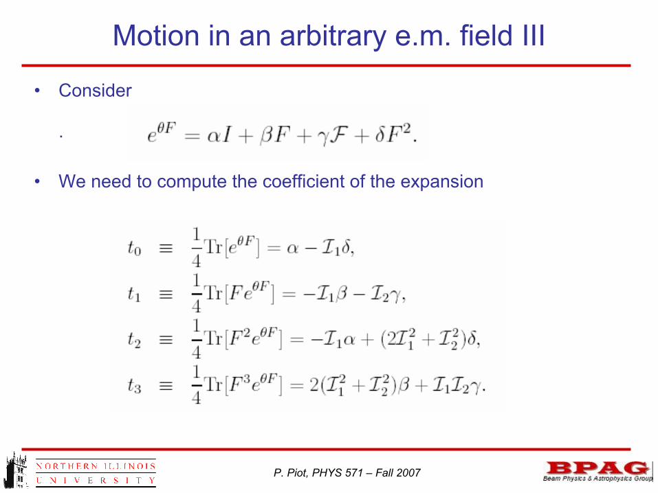
• Consider
.
• We need to compute the coefficient of the expansion
Motion in an arbitrary e.m. field III
P. Piot, PHYS 571 – Fall 2007
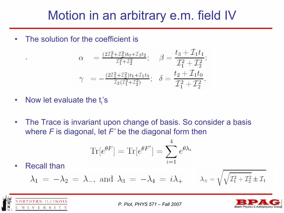
• The solution for the coefficient is
.
• Now let evaluate the ti’s
• The Trace is invariant upon change of basis. So consider a basiswhere F is diagonal, let F’ be the diagonal form then
• Recall than
Motion in an arbitrary e.m. field IV

P. Piot, PHYS 571 – Fall 2007
• The traces are then.
• Now let evaluate the ti’s
Motion in an arbitrary e.m. field V

P. Piot, PHYS 571 – Fall 2007
• The traces are then.
• Substitute in the power expansion to yield
Motion in an arbitrary e.m. field VI

P. Piot, PHYS 571 – Fall 2007
• Remember that
• Integrate for
Motion in an arbitrary e.m. field VII

P. Piot, PHYS 571 – Fall 2007
• Let’s consider the special case
• Then
• So we just take the limit in the equation motion derived in the previous slide which means:
• So we obtain
Motion in an arbitrary e.m. field VIII

P. Piot, PHYS 571 – Fall 2007
• With
• compute
ExB drift

P. Piot, PHYS 571 – Fall 2007
• With
• compute
ExB drift I
P. Piot, PHYS 571 – Fall 2007
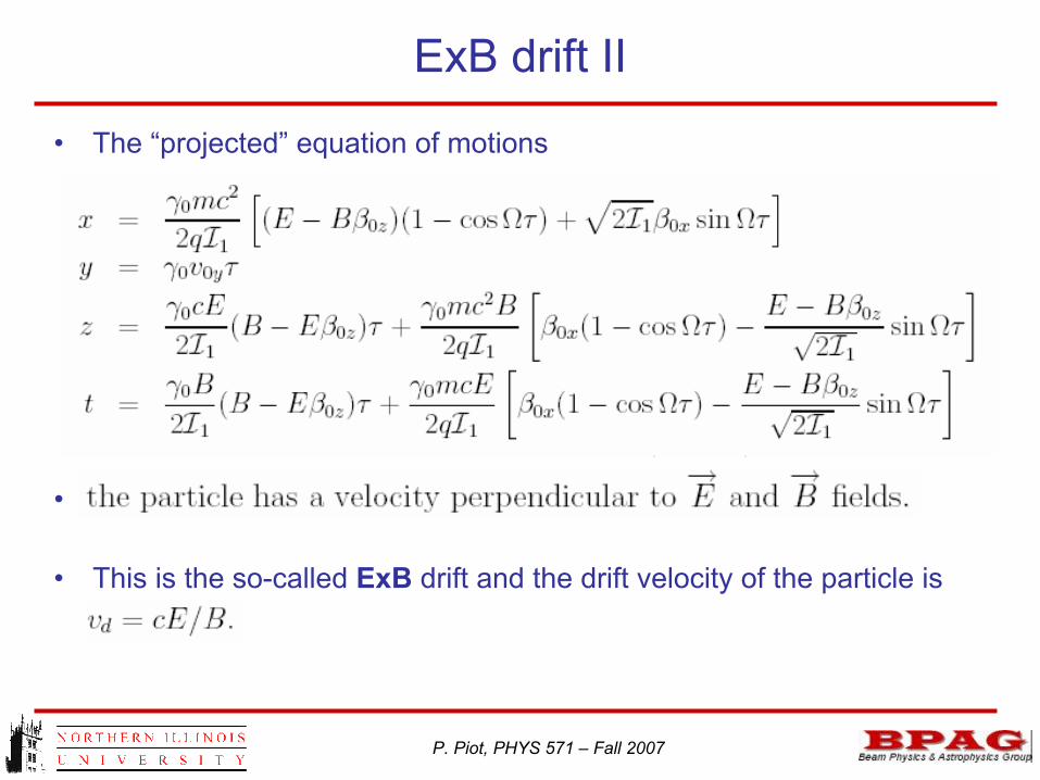
• The “projected” equation of motions
• …..
• This is the so-called ExB drift and the drift velocity of the particle is
ExB drift II

P. Piot, PHYS 571 – Fall 2007
ExB drift III