appendix a relations between covariant and contravariant bases978-3-662-43444-4/1.pdf · relations...
TRANSCRIPT

Appendix ARelations Between Covariantand Contravariant Bases
The contravariant basis vector gk of the curvilinear coordinate of uk at the pointP is perpendicular to the covariant bases gi and gj, as shown in Fig. A.1. Thiscontravariant basis gk can be defined as
a gk � gi � gj ¼or
oui� or
ou jðA:1Þ
where a is the scalar factor; gk is the contravariant basis of the curvilinearcoordinate of uk.
Multiplying Eq. (A.1) by the covariant basis gk, the scalar factor a results in
ðgi � gjÞ: gk ¼ aðgk: gkÞ ¼ a dkk ¼ a
) a ¼ ðgi � gjÞ : gk � gi; gj; gk
� � ðA:2Þ
The scalar triple product of the covariant bases can be written as
a ¼ g1; g2; g3½ � ¼ ðg1 � g2Þ : g3 ¼ffiffiffigp ¼ J ðA:3Þ
where Jacobian J is the determinant of the covariant basis tensor G.The direction of the cross product vector in Eq. (A.1) is opposite if the dummy
indices are interchanged with each other in Einstein summation convention.Therefore, the Levi-Civita permutation symbols (pseudo-tensor components) canbe used in expression of the contravariant basis.
ffiffiffigp
gk ¼ J gk ¼ ðgi � gjÞ ¼ �ðgj � giÞ
) gk ¼eijkðgi � gjÞffiffiffi
gp ¼
eijkðgi � gjÞJ
ðA:4Þ
where the Levi-Civita permutation symbols are defined by
eijk ¼þ1 if ði; j; kÞ is an even permutation;
�1 if ði; j; kÞ is an odd permutation;
0 if i ¼ j; or i ¼ k; or j ¼ k
8><
>:
, eijk ¼ 12ði� jÞ � ðj� kÞ � ðk � iÞ for i; j; k ¼ 1; 2; 3
ðA:5Þ
H. Nguyen-Schäfer and J.-P. Schmidt, Tensor Analysis and ElementaryDifferential Geometry for Physicists and Engineers, Mathematical Engineering 21,DOI: 10.1007/978-3-662-43444-4, � Springer-Verlag Berlin Heidelberg 2014
197

Thus, the cross product of the covariant bases gi and gj results from Eq. (A.4):
ðgi � gjÞ ¼ eijkffiffiffigp
gk ¼ eijkJgk � eijkgk
) gk ¼eijkðgi � gjÞffiffiffi
gp ¼ eijkðgi � gjÞ
) eijk ¼ ðgi � gjÞgk
ðA:6Þ
The covariant permutation symbols in Eq. (A.6) can be defined as
eijk ¼þ ffiffiffi
gp
if ði; j; kÞ is an even permutation;� ffiffiffi
gp
if ði; j; kÞ is an odd permutation;0 if i ¼ j; or i ¼ k; or j ¼ k
8<
:ðA:7Þ
The contravariant permutation symbols in Eq. (A.6) can be defined as
eijk ¼þ 1ffiffi
gp if ði; j; kÞ is an even permutation;
� 1ffiffigp if ði; j; kÞ is an odd permutation;
0 if i ¼ j; or i ¼ k; or j ¼ k
8<
:ðA:8Þ
The covariant basis vector gk of the curvilinear coordinate of uk at the point P isperpendicular to the contravariant bases gi and gj, as shown in Fig. A.1. Therefore,the cross product of the contravariant bases gi and gj can be written as
ðgi � g jÞ ¼ eijkffiffiffiffigp gk ¼
eijk
Jgk � eijkgk
) eijk ¼ ðgi � g jÞgkðA:9Þ
Thus, the covariant basis results from Eq. (A.9):
gk ¼ eijkffiffiffiffigp ðgi � g jÞ ¼ eijkJðgi � g jÞ
¼ eijkðgi � g jÞðA:10Þ
Obviously, there are some relations between the covariant and contravariantpermutation symbols:
eijk eijk ¼ 1 ðno summationÞeijk ¼ eijkJ2 ðno summationÞ
ðA:11Þ
g1
g 2
g 3
u1 u2
u3
P
g 3
g 1
g 2
x 3
x1 x 20
e1e2
e3
Fig. A.1 Covariant andcontravariant bases ofcurvilinear coordinates
198 Appendix A: Relations Between Covariant and Contravariant Bases

The tensor product of the covariant and contravariant permutation pseudo-tensors is a sixth-order tensor.
eijk epqr ¼ dijkpqr ¼
þ1; ði; j; kÞ and ðl;m; nÞ even permutation;�1; ði; j; kÞ and ðl;m; nÞ odd permutation;0; otherwise
8<
:ðA:12Þ
The sixth-order Kronecker tensor can be written in the determinant form:
eijk epqr ¼ dijkpqr ¼
dip di
q dir
d jp d j
q d jr
dkp dk
q dkr
�������
�������ðA:13Þ
Using the tensor contraction rules with k = r, one obtains
dijpq ¼ dijr
pqr ¼di
p diq di
r
d jp d j
q d jr
drp dr
q drr
�������
�������¼
dip di
q dir
d jp d j
q d jr
0 0 1
�������
�������
) eijepq ¼ dijpq ¼ 1 �
dip di
q
d jp d j
q
�����
�����¼ di
pdjq � di
qdjp
ðA:14Þ
Further contraction of Eq. (A.14) with j = q gives
eiqepq ¼ dipd
qq � di
qdqp
¼ dipd
qq � di
p ¼ 2dip � di
p ¼ dip for i; p ¼ 1; 2
ðA:15Þ
From Eq. (A.15), the next contraction with i = p gives
epqepq ¼ dpp ðsummation over pÞ
¼ d11 þ d2
2 ¼ 2 for p ¼ 1; 2ðA:16Þ
Similarly, contracting Eq. (A.13) with k = r; j = q, one has for a three-dimensional space.
eiqepq ¼ dipd
qq � dq
pdiq
¼ dipd
qq � di
p ¼ 3dip � di
p ¼ 2dip for i; p ¼ 1; 2; 3
ðA:17Þ
Contracting Eq. (A.17) with i = p, one obtains
epqepq ¼ 2dpp ðsummation over pÞ
¼ 2ðd11 þ d2
2 þ d33Þ
¼ 2ð1þ 1þ 1Þ ¼ 6 for p ¼ 1; 2; 3
ðA:18Þ
Appendix A: Relations Between Covariant and Contravariant Bases 199

The covariant metric tensor M can be written as
M ¼g11 g12 g13
g21 g22 g23
g31 g32 g33
2
4
3
5 ðA:19Þ
where the covariant metric coefficients are defined by gij ¼ gi � gj.The contravariant metric coefficients in the contravariant metric tensor M-1
result from inverting the covariant metric tensor M.
M�1 ¼g11 g12 g13
g21 g22 g23
g31 g32 g33
2
4
3
5 ðA:20Þ
where the contravariant metric coefficients are defined by gij ¼ gi � g j.Thus, the relation between the covariant and contravariant metric coefficients
can be written as
gikgkj ¼ gkjgik ¼ di
j ,M�1M ¼MM�1 ¼ I ðA:21Þ
In the case of i 6¼ j, all terms of gikgkj equal zero. Thus, only nine terms of gikgki
for i = j remain in a three-dimensional space R3:
gikgki ¼ g1kgk1 þ g2kgk2 þ g3kgk3 for i; k ¼ 1; 2; 3
¼ d11 þ d2
2 þ d33 ¼ di
i for i ¼ 1; 2; 3
¼ 1þ 1þ 1 ¼ 3
ðA:22Þ
The relation between the covariant and contravariant bases in the generalcurvilinear coordinates results in
gi:gj ¼ gikgkj ¼ dij for i � j
) gi:gi ¼ g1:g1 þ g2:g2 þ g3:g3 for i ¼ 1; 2; 3¼ gikgki ¼ di
i for i; k ¼ 1; 2; 3ðA:23Þ
According to Eq. (A.23), nine terms of gikgki for k = 1, 2, 3 result in
g1 � g1 ¼ g1kgk1 ¼ g11g11 þ g12g21 þ g13g31 ¼ d11 for i ¼ 1;
g2 � g2 ¼ g2kgk2 ¼ g21g12 þ g22g22 þ g23g32 ¼ d22 for i ¼ 2;
g3 � g3 ¼ g3kgk3 ¼ g31g13 þ g32g23 þ g33g33 ¼ d33 for i ¼ 3:
8><
>:ðA:24Þ
The scalar product of the covariant and contravariant bases gives
gðiÞ � gðiÞ ¼ gðiÞ�� �� � gðiÞ
������ cosð gðiÞ; gðiÞÞ
¼ffiffiffiffiffiffiffiffigðiiÞ
q� ffiffiffiffiffiffiffiffi
gðiiÞp
cosðgðiÞ; gðiÞÞ ¼ 1ðA:25Þ
where the index (i) means no summation is carried out over i.
200 Appendix A: Relations Between Covariant and Contravariant Bases
Equation (A.25) indicates that the product of the covariant and contravariantbasis norms generally does not equal one in the curvilinear coordinates.
ffiffiffiffiffiffiffiffigðiiÞ
q� ffiffiffiffiffiffiffiffi
gðiiÞp ¼ 1
cosð gðiÞ; gðiÞÞ� 1 ðA:26Þ
In orthogonal coordinate systems, g(i) is parallel to g(i). Therefore, Eq. (A.26)becomes
ffiffiffiffiffiffiffiffigðiiÞ
q� ffiffiffiffiffiffiffiffi
gðiiÞp ¼ 1)
ffiffiffiffiffiffiffiffigðiiÞ
q¼ 1
ffiffiffiffiffiffiffiffigðiiÞp ¼ 1
hiðA:27Þ
Appendix A: Relations Between Covariant and Contravariant Bases 201

Appendix BPhysical Components of Tensors
The physical component of a tensor can be defined as the tensor component on itsunitary covariant basis. Therefore, the covariant basis of the general curvilinearcoordinates has to be normalized.
Dividing the covariant basis by its vector length, the unitary covariant basis(covariant-normalized basis) results in
g�i ¼gi
gij j¼ giffiffiffiffiffiffiffiffi
gðiiÞp ) g�i
�� �� ¼ 1 ðB:1aÞ
The covariant basis norm |gi| can be considered as a scale factor hi withoutsummation over (i).
hi ¼ gij j ¼ffiffiffiffiffiffiffiffigðiiÞp ðB:1bÞ
Thus, the covariant basis can be related to its unitary covariant basis by therelation
gi ¼ffiffiffiffiffiffiffiffigðiiÞp
g�i ¼ hig�i ðB:2Þ
The contravariant basis can be related to its unitary covariant basis using Eqs.(2.47 and B.2).
gi ¼ gijgj ¼ gijhjg�j ðB:3Þ
The contravariant second-order tensor can be written in the unitary covariantbases using Eq. (B.2).
T ¼ Tijgigj ¼ ðTijhihjÞ g�i g�j � T�ijg�i g�j ðB:4Þ
Thus, the physical contravariant tensor components denoted by star result in
T�ij � hihjTij ðB:5Þ
The covariant second-order tensor can be written in the unitary contravariantbases using Eq. (B.3).
T ¼ Tijgig j ¼ ðTijg
ikgjlhkhlÞ g�kg�l � T�ijg�kg�l ðB:6Þ
H. Nguyen-Schäfer and J.-P. Schmidt, Tensor Analysis and ElementaryDifferential Geometry for Physicists and Engineers, Mathematical Engineering 21,DOI: 10.1007/978-3-662-43444-4, � Springer-Verlag Berlin Heidelberg 2014
203

Similarly, the physical covariant tensor components denoted by star result in
T�ij � gikgjlhkhlTij ðB:7Þ
The mixed tensors can be written in the unitary covariant bases using Eqs. (B.2and B.3)
T ¼ Tij gig
j ¼ Tij giðgjkgkÞ
¼ Tij ðhig
�i Þðgjkhkg�kÞ
¼ ðTij g
jkhihkÞg�i g�k
� ðTij Þ�g�i g�k
ðB:8Þ
Thus, the physical mixed tensor components denoted by star result in
ðTij Þ� � gjkhihkTi
j ðB:9Þ
Analogously, the contravariant vector can be written using Eq. (B.2).
v ¼ vigi ¼ ðvihiÞg�i
� v�ig�i ¼v�i
higi
ðB:10Þ
Thus, the physical component of the contravariant vector v on the unitary basisgi
* is defined as
v�i � hivi ¼ ffiffiffiffiffiffiffiffi
gðiiÞp
vi ðB:11Þ
The contravariant basis can be normalized dividing by its vector length withoutsummation over (i).
g�i ¼ gi
gij j ¼gi
ffiffiffiffiffiffiffiffigðiiÞ
p ðB:12Þ
where g(ii) is the contravariant metric coefficient that results from Eq. (A.20).Using Eq. (B.12), the covariant vector v can be written as
v ¼ vigi ¼ vi
ffiffiffiffiffiffiffiffigðiiÞ
qg�i � v�i g�i ðB:13Þ
Thus, the physical component of the covariant vector v results in
v�i ¼ vi
ffiffiffiffiffiffiffiffigðiiÞ
qðB:14Þ
According to Eq. (A.27), Eq. (B.14) can be rewritten in orthogonal coordinatesystems:
v�i ¼ffiffiffiffiffiffiffiffigðiiÞ
qvi ¼
1ffiffiffiffiffiffiffiffigðiiÞp vi ¼
1hi
vi ðB:15Þ
204 Appendix B: Physical Components of Tensors

Using Eq. (B.3), the covariant vector can be written in
v ¼ vigi ¼ vig
ijgj
¼ ðvigijhjÞg�j � v�j g�j
¼v�j
gijhjgi
ðB:16Þ
Thus, the physical contravariant vector component of v on the unitary basis gj*
can be defined as
v�j � gijhjvi ðB:17Þ
Furthermore, the vector v can be written in both covariant and contravariantbases.
v ¼ vjgj ¼ vigi
) ðvjgjÞ:gk ¼ ðvigiÞ:gk
) vjdjk ¼ vigik
) vk ¼ vigik
ðB:18Þ
Interchanging i with j and k with i, one obtains
vi ¼ v jgij ðB:19Þ
Only in orthogonal coordinate systems, we have
gij ¼ 0 for i 6¼ j; gðiiÞ ¼ h2i ðB:20Þ
Thus, one obtains from Eq. (B.19)
vi ¼ v jgij ¼ v1gi1 þ v2gi2 þ � � � þ vNgiN
¼ vigðiiÞ ¼ vih2i
ðB:21Þ
Substituting Eq. (B.11) into Eq. (B.21), one obtains Eq. (B.22) that is equivalentto Eq. (B.15).
vi ¼ vih2i ¼
v�i
hi
� �h2
i ¼ hiv�i ðB:22Þ
Appendix B: Physical Components of Tensors 205

Appendix CNabla Operators
Some useful Nabla operators are listed in Cartesian and general curvilinearcoordinates:
1. Gradient of an invariant f
• Cartesian coordinate {xi}
rf ¼ of
oxex þ
of
oyey þ
of
ozez ðC:1Þ
• General curvilinear coordinate {ui}
rf ¼ f;igi ¼ of
ouigi ¼ of
ouigijgj ðC:2Þ
2. Gradient of a vector v
• General curvilinear coordinate {ui}
rv ¼ vk;i þ v jCk
ij
� gkgi ¼ vk
��igkgi
¼ vk;i � vjCjik
�gkgi ¼ vkjigkgi
ðC:3Þ
3. Divergence of a vector v
• Cartesian coordinate {xi}
r � v ¼ ovx
oxþ ovy
oyþ ovz
ozðC:4Þ
H. Nguyen-Schäfer and J.-P. Schmidt, Tensor Analysis and ElementaryDifferential Geometry for Physicists and Engineers, Mathematical Engineering 21,DOI: 10.1007/978-3-662-43444-4, � Springer-Verlag Berlin Heidelberg 2014
207
• General curvilinear coordinate {ui}
r:v ¼ viij � ðvi
;i þ v jCiijÞ
¼ 1J
oðJviÞoui
¼ J�1ðJviÞ;ir � v ¼ vk ij gki ¼ ðvk;i � vjC
jikÞgk � gi
ðC:5Þ
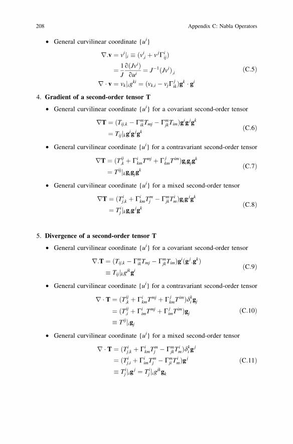
4. Gradient of a second-order tensor T
• General curvilinear coordinate {ui} for a covariant second-order tensor
rT ¼ ðTij;k � CmikTmj � Cm
jkTimÞgig jgk
¼ Tij kj gig jgkðC:6Þ
• General curvilinear coordinate {ui} for a contravariant second-order tensor
rT ¼ ðTij;k þ Ci
kmTmj þ C jkmTimÞgigjg
k
¼ T ijkj gigjg
kðC:7Þ
• General curvilinear coordinate {ui} for a mixed second-order tensor
rT ¼ ðTij;k þ Ci
kmTmj � Cm
jkTimÞgig
jgk
¼ Tij kj gig
jgkðC:8Þ
5. Divergence of a second-order tensor T
• General curvilinear coordinate {ui} for a covariant second-order tensor
r:T ¼ ðTij;k � CmikTmj � Cm
jkTimÞgiðg j:gkÞ� Tij kj gjkgi
ðC:9Þ
• General curvilinear coordinate {ui} for a contravariant second-order tensor
r � T ¼ ðTij;k þ Ci
kmTmj þ C jkmTimÞdk
i gj
¼ ðTij;i þ Ci
imTmj þ C jimTimÞgj
� Tijij gj
ðC:10Þ
• General curvilinear coordinate {ui} for a mixed second-order tensor
r � T ¼ ðTij;k þ Ci
kmTmj � Cm
jkTimÞdk
i g j
¼ ðTij;i þ Ci
imTmj � Cm
ji TimÞg j
� Tij ij g j ¼ Ti
j ij gjkgk
ðC:11Þ
208 Appendix C: Nabla Operators

6. Curl of a vector v
• Cartesian coordinate {xi}
r� v ¼ex ey ezoox
ooy
ooz
vx vy vz
������
������ðC:12Þ
The curl of v results from calculating the determinant of Eq. (C.12).
r� v ¼ ovz
oy� ovy
oz
� �ex þ
ovx
oz� ovz
ox
� �ey þ
ovy
ox� ovx
oy
� �ez ðC:13Þ
• General curvilinear coordinate {ui}
r� v ¼ eijkvj;igk ðC:14Þ
The contravariant permutation symbol is defined by
eijk ¼þJ�1 if ði; j; kÞ is an even permutation;�J�1 if ði; j; kÞ is an odd permutation;0 if i ¼ j; or i ¼ k; or j ¼ k
8<
:ðC:15Þ
where J is the Jacobian.
7. Laplacian of an invariant f
• Cartesian coordinate {xi}
r2f � Df ¼ o2f
ox2þ o2f
oy2þ o2f
oz2ðC:16Þ
• General curvilinear coordinate {ui}
r2f � Df ¼ ðf;ij � f;kCkijÞgij
¼ ðvi;j � vkCkijÞgij � vi j
�� gijðC:17Þ
where the covariant vector component and its covariant derivative withrespect to uk are defined by
vi ¼ f;i ¼of
oui; vk ¼ f;k ¼
of
ouk; vi;j ¼ f;ij ¼
o2f
ouiou jðC:18Þ
Appendix C: Nabla Operators 209

8. Calculation rules of the Nabla operators
Div Grad f ¼ r � ðrf Þ ¼ r2f ¼ Df Laplacianð Þ ðC:19Þ
Curl Grad f ¼ r� ðrf Þ ¼ 0 ðC:20Þ
Div Curl v ¼ r � ðr � vÞ ¼ 0 ðC:21Þ
DðfgÞ ¼ f Dgþ 2rf � rgþ gDf ðC:22Þ
Curl Curl v ¼ r� ðr � vÞ ¼ rðr � vÞ � Dv Curl identityð Þ ðC:23Þ
The Laplacian of v in Eq. (C.23) is computed in the tensor formulation forgeneral curvilinear coordinates.
Div Grad v ¼ Laplacian v ¼ Dv
¼ r � ðrvÞ ¼ r2v
¼ ðvij;k
�� � vip
�� Cpjk þ vp
j
�� CipkÞgjkgi
� vijk
�� gjkgi
ðC:24Þ
210 Appendix C: Nabla Operators

Appendix DEssential Tensors
Derivative of the covariant basis
gi;j ¼ Ckijgk ðD:1Þ
Derivative of the contravariant basis
gi;j ¼
ogi
ou j� Ci
jkgk ¼ �Cijkgk ðD:2Þ
Derivative of the covariant metric coefficient
gij;k ¼ Cpikgpj þ Cp
jkgp i ðD:3Þ
First-kind Christoffel symbol
Cijk ¼ 12ðgik;j þ gjk;i � gij;k Þ ¼ glkC
lij
) Clij ¼ glkCijk
ðD:4Þ
Second-kind Christoffel symbol based on the covariant basis
Ckij ¼ gi;j � gk ¼ gklCijl ðD:5Þ
Ckij ¼
ouk
oxp� o2xp
ouiou j¼ Ck
ji ðD:6Þ
Ckij ¼ gkp1
2ðgip;j þ gjp;i � gij;pÞ ðD:7Þ
Ciij ¼
1J
oJ
ou j¼ oðln JÞ
ou jðD:8Þ
Second-kind Christoffel symbol based on the contravariant basis
Cikj ¼ �Ci
kj ¼ Cijk ðD:9Þ
H. Nguyen-Schäfer and J.-P. Schmidt, Tensor Analysis and ElementaryDifferential Geometry for Physicists and Engineers, Mathematical Engineering 21,DOI: 10.1007/978-3-662-43444-4, � Springer-Verlag Berlin Heidelberg 2014
211

Covariant derivative of covariant first-order tensors
Ti j
�� ¼ Ti;j � CkijTk ¼ T;j � gi ðD:10Þ
Covariant derivative of contravariant first-order tensors
Tij
�� ¼ Ti;j þ Ci
jkTk ¼ T;j � gi ðD:11Þ
Covariant derivative of covariant and contravariant second-order tensors
Tij kj ¼ Tij;k � CmikTmj � Cm
jkTim
Tijkj ¼ Tij
;k þ CikmTmj þ C j
kmTimðD:12Þ
Covariant derivative of mixed second-order tensors
Tij kj ¼ Ti
j;k þ CikmTm
j � CmjkTi
m
T ji kj ¼ T j
i;k þ C jkmTm
i � CmikT j
m
ðD:13Þ
Second covariant derivative of covariant first-order tensors
Ti kj
�� ¼ Ti;jk � Cmik;jTm � Cm
ikTm;j
� Cmij Tm;k þ Cm
ij CnmkTn
� CmjkTi;m þ Cm
jkCnimTn
ðD:14Þ
Second covariant derivative of the contravariant vector
vklmj � vk
l;m
�� � vkp
�� Cplm þ vp
lj Ckpm ðD:15Þ
where
vkl;m ¼�� vk
lj �
;m� vk;lm þ vn
;mCknl þ vnCk
nl;m ðD:16Þ
vkp
�� � vk;p þ vnCk
np ðD:17Þ
vplj � vp
;l þ vnCpnl ðD:18Þ
Riemann–Christoffel tensor
Rnijk � Cn
ik;j � Cnij;k þ Cm
ikCnmj � Cm
ij Cnmk ðD:19Þ
Riemann curvature tensor
Rlijk � glnRnijk ðD:20Þ
212 Appendix D: Essential Tensors

First-kind Ricci tensor
Rij ¼oCk
ik
ou j�
oCkij
ouk� Cr
ijCkrk þ Cr
ikCkrj
¼ o2ðln JÞouiou j
� 1J
oðJCkijÞ
oukþ Cr
ikCkrj
ðD:21Þ
Second-kind Ricci tensor
Rij � gikRkj
¼ gik o2ðln JÞoukou j
� 1J
oðJCmkjÞ
oumþ Cm
knCnmj
� � ðD:22Þ
Ricci curvature
R ¼ gij o2ðln JÞouiou j
� 1J
oðJCkijÞ
oukþ Ck
irCrkj
!
ðD:23Þ
Einstein tensor
Gij � Ri
j �12di
jR ¼ gikGkj
Gij ¼ gikGkj ¼ Rij � 1
2gijR
ðD:24Þ
Gij
���i¼ 0 ðD:25Þ
First fundamental form
I ¼ Edu2 þ 2Fdudvþ Gdv2;
M ¼ ðgijÞ �E F
F G
� ¼
ruru rurv
rvru rvrv
� ðD:26Þ
Second fundamental form
II ¼ Ldu2 þ 2Mdudvþ Ndv2;
H ¼ ðhijÞ �L M
M N
� ¼
ruun ruvn
ruvn rvvn
� ðD:27Þ
Gaussian curvature of a curvilinear surface
K ¼ j1j2 ¼LN �M2
EG� F2¼ detðhijÞ
detðgijÞðD:28Þ
Mean curvature of a curvilinear surface
H ¼ 12ðj1 þ j2Þ ¼
EN � 2MF þ LG
2ðEG� F2Þ ðD:29Þ
Appendix D: Essential Tensors 213

Unit normal vector of a curvilinear surface
n ¼ g1 � g2
g1 � g2j j ¼ru � rvffiffiffiffiffiffiffiffiffiffiffiffiffiffiffidetðgijÞ
p ¼ ru � rvffiffiffiffiffiffiffiffiffiffiffiffiffiffiffiffiffiffiEG� F2p ðD:30Þ
Differential of a surface area
dA ¼ g1 � g2j jdudv ¼ffiffiffiffiffiffiffiffiffiffiffiffiffiffiffiffiffiffiffiffiffiffiffiffiffiffiffiffiffiffig11g22 � ðg12Þ2
qdudv
¼ffiffiffiffiffiffiffiffiffiffiffiffiffiffiffidetðgijÞ
qdudv ¼
ffiffiffiffiffiffiffiffiffiffiffiffiffiffiffiffiffiffiEG� F2p
dudvðD:31Þ
Gauss derivative equations
gi;j ¼ Ckijgk þ hijg3 ¼ Ck
ijgk þ hijn
, gi j
�� � gi;j � Ckijgk ¼ hijn
ðD:32Þ
Weingarten’s equations
ni ¼ �h ji gj ¼ �ðhikgjkÞgj ðD:33Þ
Codazzi’s equations
Kij;k ¼ Kik;j ) ðK11;2 ¼ K12;1 ; K21;2 ¼ K22;1Þ ðD:34Þ
Gauss equations
K ¼ det ðK ji Þ ¼ ðK1
1 K22 � K1
2 K21Þ
¼ K11K22 � K212
g11g22 � g212
¼ R1212
g
ðD:35Þ
214 Appendix D: Essential Tensors

Appendix EEuclidean and Riemannian Manifolds
In the following appendix, we summarize fundamental notations and basic resultsfrom vector analysis in Euclidean and Riemannian manifolds. This section can bewritten informally and is intended to remind the reader of some fundamentals ofvector analysis in general curvilinear coordinates. For the sake of simplicity, weabstain from being mathematically rigorous. Therefore, we recommend someliterature given in References for the mathematically interested reader.
E.1 N-dimensional Euclidean Manifold
N-dimensional Euclidean manifold EN can be represented by two kinds ofcoordinate systems: Cartesian (orthonormal) and curvilinear (non-orthogonal)coordinate systems with N dimensions. Lines, curves, and surfaces can beconsidered as subsets of Euclidean manifold. Two lines or two curves can generatea flat (planes) and curvilinear surface (cylindrical and spherical surfaces),respectively. Both kinds of surfaces can be embedded in Euclidean space.
E.1.1 Vector in Cartesian Coordinates
Cartesian coordinates are an orthonormal coordinate system in which the bases(i, j, k) are mutually perpendicular (orthogonal) and unitary (normalized vectorlength). The orthonormal bases (i, j, k) are fixed in Cartesian coordinates. Anyvector could be described by its components and the relating bases in Cartesiancoordinates.
The vector r can be written in Euclidean space E3 (three-dimensional space) inCartesian coordinates (cf. Fig. E.1).
r ¼ xiþ yjþ zk ðE:1Þ
H. Nguyen-Schäfer and J.-P. Schmidt, Tensor Analysis and ElementaryDifferential Geometry for Physicists and Engineers, Mathematical Engineering 21,DOI: 10.1007/978-3-662-43444-4, � Springer-Verlag Berlin Heidelberg 2014
215

where
x, y, z are the vector components in the coordinate system (x, y, z);i, j, k are the orthonormal bases of the corresponding coordinates.
The vector length of r can be computed using the Pythagorean theorem as
rj j ¼ffiffiffiffiffiffiffiffiffiffiffiffiffiffiffiffiffiffiffiffiffiffiffiffiffiffix2 þ y2 þ z2
p� 0 ðE:2Þ
E.1.2 Vector in Curvilinear Coordinates
We consider a curvilinear coordinate system (u1, u2, u3) of Euclidean space E3,i.e., a coordinate system which is generally non-orthogonal and non-unitary (non-orthonormal basis). By abuse of notation, we denote the basis vector simply basis.
In other words, the bases are not mutually perpendicular and their vectorlengths are not equal to one (Klingbeil 1966; Nayak 2012). In the curvilinearcoordinate system (u1, u2, u3), there are three covariant bases g1, g2, and g3 andthree contravariant bases g1, g2, and g3 at the origin 00, as shown in Fig. E.2.Generally, the origin 00 of the curvilinear coordinates could move everywhere inEuclidean space; therefore, the bases of the curvilinear coordinates only depend on
z
x
y
r
0
x
y
z
ij
k
P(x,y,z)
y j
zk
x i
(xi +y j)
zk
Fig. E.1 Vector r inCartesian coordinates
g 1
g 2
g 3
u1 u2
u3
P(u1,u2,u3)
r
0‘
g 3
g1
g 2
Fig. E.2 Bases of thecurvilinear coordinates
216 Appendix E: Euclidean and Riemannian Manifolds
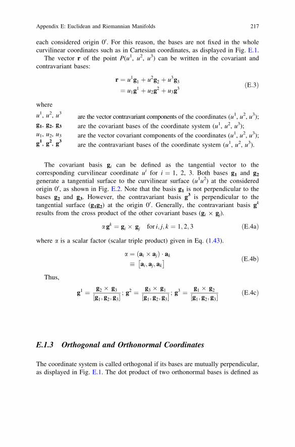
each considered origin 00. For this reason, the bases are not fixed in the wholecurvilinear coordinates such as in Cartesian coordinates, as displayed in Fig. E.1.
The vector r of the point P(u1, u2, u3) can be written in the covariant andcontravariant bases:
r ¼ u1g1 þ u2g2 þ u3g3
¼ u1g1 þ u2g2 þ u3g3ðE:3Þ
where
u1, u2, u3are the vector contravariant components of the coordinates (u1, u2, u3);
g1, g2, g3 are the covariant bases of the coordinate system (u1, u2, u3);u1, u2, u3 are the vector covariant components of the coordinates (u1, u2, u3);g1, g2, g3
are the contravariant bases of the coordinate system (u1, u2, u3).
The covariant basis gi can be defined as the tangential vector to thecorresponding curvilinear coordinate ui for i = 1, 2, 3. Both bases g1 and g2
generate a tangential surface to the curvilinear surface (u1u2) at the consideredorigin 00, as shown in Fig. E.2. Note that the basis g1 is not perpendicular to thebases g2 and g3. However, the contravariant basis g3 is perpendicular to thetangential surface (g1g2) at the origin 00. Generally, the contravariant basis gk
results from the cross product of the other covariant bases (gi 9 gj).
a gk ¼ gi � gj for i; j; k ¼ 1; 2; 3 ðE:4aÞ
where a is a scalar factor (scalar triple product) given in Eq. (1.43).
a ¼ ðai � ajÞ � ak
� ai; aj; ak
� � ðE:4bÞ
Thus,
g1 ¼ g2 � g3
g1; g2; g3½ � ; g2 ¼ g3 � g1
g1; g2; g3½ � ; g3 ¼ g1 � g2
g1; g2; g3½ � ðE:4cÞ
E.1.3 Orthogonal and Orthonormal Coordinates
The coordinate system is called orthogonal if its bases are mutually perpendicular,as displayed in Fig. E.1. The dot product of two orthonormal bases is defined as
Appendix E: Euclidean and Riemannian Manifolds 217

i : j ¼ ij j � jj j � cos ði; jÞ
¼ ð1Þ � ð1Þ � cosp2
�
¼ 0
ðE:5Þ
Thus,
i � j ¼ i � k ¼ j � k ¼ 0 ðE:6Þ
If the length of each basis equals 1, the bases are unitary vectors.
ij j ¼ jj j ¼ kj j ¼ 1 ðE:7Þ
If the coordinate system satisfies both conditions (E.6) and (E.7), it is called theorthonormal coordinate system, which exists in Cartesian coordinates.
Therefore, the vector length in the orthonormal coordinate system results from
rj j2 ¼ r � r¼ x iþ y jþ zkð Þ � xiþ y jþ z kð Þ¼ x2ði � iÞ þ xyði � jÞ þ xzði � kÞþ yxðj � iÞ þ y2ðj � jÞ þ yzðj � kÞþ zxðk � iÞ þ zyðk � jÞ þ z2ðk � kÞ
ðE:8Þ
Due to Eqs. (E.6 and E.7), the vector length in Eq. (E.8) becomes
rj j2¼ x2 þ y2 þ z2 ) rj j ¼ffiffiffiffiffiffiffiffiffiffiffiffiffiffiffiffiffiffiffiffiffiffiffiffix2 þ y2 þ z2
pðE:9Þ
The cross product (called vector product) of a pair of bases of the orthonormalcoordinate system is (informally) given by means of right-handed rule; that is, ifthe right-hand fingers move in the rotating direction from the basis j to the basis k,the thumb will point in the direction of the basis i = j 9 k. The bases (i, j, k) forma right-handed triple.
i ¼ j� k ¼ �k � j
j ¼ k� i ¼ �i � k
k ¼ i� j ¼ �j � i
8><
>:ðE:10Þ
The cross product of two orthonormal bases can be defined as
i� jj j ¼ ij j � jj j � sinði; jÞ
¼ ð1Þ � ð1Þ � sinp2
�
¼ kj j
ðE:11Þ
218 Appendix E: Euclidean and Riemannian Manifolds

E.1.4 Arc Length Between Two Points in a Euclidean Manifold
We consider two points P(x1, x2, x3) and Q(x1, x2, x3) in Euclidean space E3 inCartesian and curvilinear coordinate systems, as shown in Figs. E.3 and E.4. Bothpoints P and Q have three components x1, x2, and x3 in Cartesian coordinates (e1,e2, e3). To simplify some mathematically written expressions, the coordinates x, y,and z in Cartesian coordinates can be transformed into x1, x2, and x3; the bases (i, j,k) turn to (e1, e2, e3).
We now turn to the notation of the differential dr of a vector r. The differentialdr can be expressed using the Einstein summation convention (Klingbeil 1966;Kay 2011):
dr � eidxi for i ¼ 1; 2; 3
¼X3
i¼1
eidxiðE:12Þ
The Einstein summation convention used in Eq. (E.12) indicates that dr equalsthe sum of ei dxi by running the dummy index i from 1 to 3.
x3
x1
x 2
r
0
x1
x 2
x 3
e1
e2
e3
P
r + dr
dr Q
(C)
ds
Fig. E.3 Arc length ds ofP and Q in Cartesiancoordinates
P(u i(t1),…)
Q(ui(t2),…)
ds
dr
r + dr
r
u1 u2
u 3
0‘(C)
g 3
g1
g 2
Fig. E.4 Arc length ds ofP and Q in the curvilinearcoordinates
Appendix E: Euclidean and Riemannian Manifolds 219

The arc length ds between the points P and Q (cf. Fig. E.3) can be calculated bythe dot product of two differentials.
ðdsÞ2 ¼ dr � dr
¼ ðeidxiÞ � ðejdx jÞ¼ ðei � ejÞdxi � dx j
¼ dxi � dxi for i ¼ 1; 2; 3:
ðE:13Þ
Thus, the arc length in the orthonormal coordinate system results in
ds ¼ffiffiffiffiffiffiffiffiffiffiffiffiffiffiffiffidxi � dxip
for i ¼ 1; 2; 3:
¼ffiffiffiffiffiffiffiffiffiffiffiffiffiffiffiffiffiffiffiffiffiffiffiffiffiffiffiffiffiffiffiffiffiffiffiffiffiffiffiffiffiffiffiffiffiffiffiffiðdx1Þ2 þ ðdx2Þ2 þ ðdx3Þ2
q ðE:14Þ
The points P and Q have three components u1, u2, and u3 in the curvilinearcoordinate system with the basis (g1, g2, g3) in Euclidean 3-space, as displayed inFig. E.4. The location vector r(u1,u2,u3) of the point P is a function of ui.Therefore, the differential dr of the vector r can be rewritten in a linearformulation of dui.
dr ¼ or
ouidui
� giduiðE:15Þ
where gi is the covariant basis of the curvilinear coordinate ui.Analogously, the arc length ds between two points of and Q in the curvilinear
coordinate system can be calculated by
ðdsÞ2 ¼ dr � dr
¼ ðgiduiÞ � ðgjdu jÞ¼ ðgi � gjÞ dui � du j
¼ gij dxi � dx j for i; j ¼ 1; 2; 3
ðE:16Þ
Therefore,
ds ¼ffiffiffiffiffiffiffiffiffiffiffiffiffiffiffiffiffiffiffiffiffiffiffiffiffigij dxi � dx j�� ��
q
) s ¼Zt2
t1
ffiffiffiffiffiffiffiffiffiffiffiffiffiffiffiffiffiffiffiffiffiffiffiffiffiffi
gijdxi
dt� dx j
dt
����
����
s
dtðE:17Þ
where
t is the parameter in the curve C with the coordinate ui(t);gij is the defined as the metric coefficient of two non-orthonormal bases.
220 Appendix E: Euclidean and Riemannian Manifolds
gij ¼ gi � gj ¼ gj � gi ¼ gji 6¼ d ji ðE:18Þ
It is obvious that the symmetric metric coefficients gij vanish for any i 6¼ j in theorthogonal bases because gi is perpendicular to gj; therefore, the metric tensor canbe rewritten as
gij ¼0 if i 6¼ jgii if i ¼ j
�ðE:19Þ
In the orthonormal bases, the metric coefficients gij in Eq. (E.19) become
gij � d ji ¼
0 if i 6¼ j1 if i ¼ j
�ðE:20Þ
where d ji is called the Kronecker delta.
E.1.5 Bases of the Coordinates
The vector r can be rewritten in Cartesian coordinates of Euclidean space E3.
r ¼ xiei ðE:21Þ
The differential dr results from Eq. (E.21) in
dr ¼ eidxi
¼ or
oxidxi
ðE:22Þ
Thus, the orthonormal bases ei of the coordinate xi can be defined as
ei ¼or
oxifor i ¼ 1; 2; 3 ðE:23Þ
Analogously, the basis of the curvilinear coordinate ui can be calculated in thecurvilinear coordinate system of E3.
gi ¼or
ouifor i ¼ 1; 2; 3 ðE:24Þ
Substituting Eq. (E.24) into Eq. (E.18), we obtain the metric coefficients gij thatare generally symmetric in Euclidean space; that is, gij = gji.
Appendix E: Euclidean and Riemannian Manifolds 221
gij ¼ gi � gj ¼ gji 6¼ d ji
¼ or
oui:or
ou j¼ or
oxm
oxm
oui
� �:
or
oxn
oxn
ou j
� �
¼ oxm
oui
oxn
ou jðem: enÞ ¼
oxm
oui
oxn
ou jdn
m
¼ oxk
oui
oxk
ou jfor k ¼ 1; 2; 3
ðE:25Þ
According to Eqs. (E.4a and E.4b), the contravariant basis gk is perpendicular toboth covariant bases gi and gj. Additionally, the contravariant basis gk is chosensuch that the vector length of the contravariant basis equals the inversed vectorlength of its relating covariant basis; thus, gk � gk ¼ 1. As a result, the scalarproducts of the covariant and contravariant bases can be written in generalcurvilinear coordinates (u1,…, uN).
gi � gk ¼ gk � gi ¼ dki for i; k ¼ 1; 2; . . .;N
gi � gk ¼ gik ¼ gki 6¼ dki for i; k ¼ 1; 2; . . .;N
(
ðE:26Þ
E.1.6 Orthonormalizing a Non-orthonormal Basis
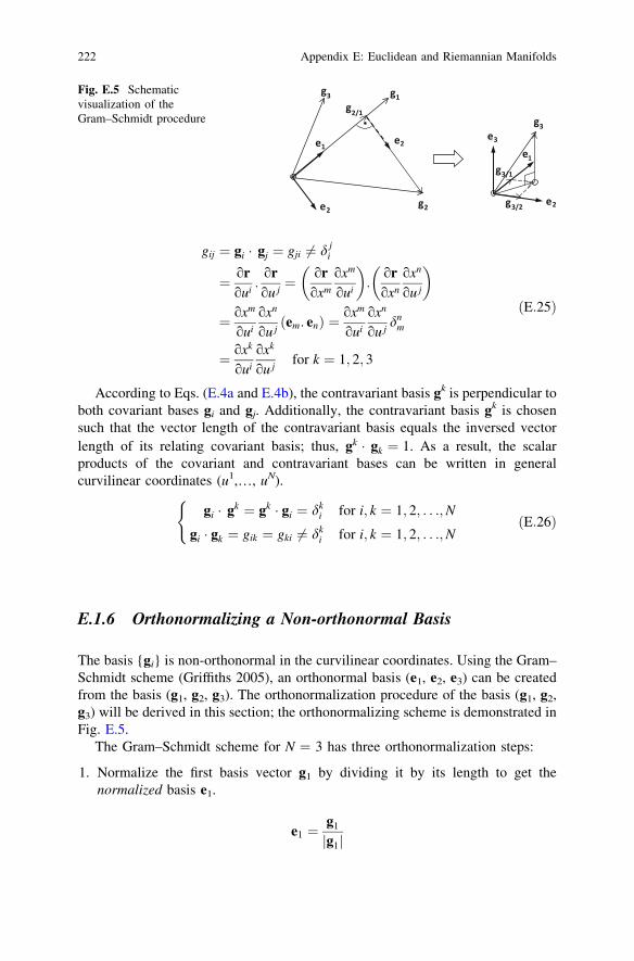
The basis {gi} is non-orthonormal in the curvilinear coordinates. Using the Gram–Schmidt scheme (Griffiths 2005), an orthonormal basis (e1, e2, e3) can be createdfrom the basis (g1, g2, g3). The orthonormalization procedure of the basis (g1, g2,g3) will be derived in this section; the orthonormalizing scheme is demonstrated inFig. E.5.
The Gram–Schmidt scheme for N = 3 has three orthonormalization steps:
1. Normalize the first basis vector g1 by dividing it by its length to get thenormalized basis e1.
e1 ¼g1
g1j j
e1
g1
g2
g3
e2
e2
g2/1g3
e3
e2
e1
g3/1
g3/2
Fig. E.5 Schematicvisualization of theGram–Schmidt procedure
222 Appendix E: Euclidean and Riemannian Manifolds

2. Project the basis g2 onto the basis g1 to get the projection vector g2/1 on thebasis g1. The normalized basis e2 results from subtracting the projection vectorg2/1 from the basis g2. Then, iteratively, normalize this vector by dividing it byits length to generate the basis e2.
e2 ¼g2 � g2=1
g2 � g2=1
������¼ g2 � ðg2 � e1Þe1
g2 � ðg2 � e1Þe1j j
3. Subtract projections along the bases of e1 and e2 from the basis g3 andnormalize it to obtain the normalized basis e3.
e3 ¼g3 � g3=1 � g3=2
g3 � g3=1 � g3=2
������¼ g3 � ðg3 � e1Þe1 � ðg3 � e2Þe2
g3 � ðg3 � e1Þe1 � ðg3 � e2Þe2j j
Using the Gram–Schmidt scheme, the orthonormal basis {e1, e2, e3} resultsfrom the non-orthonormal bases {g1, g2, g3}.
Generally, the orthogonal bases {e1, e2, …, eN} for the N-dimensional space canbe generated from the non-orthonormal bases {g1, g2, …, gN} according to theGram–Schmidt scheme as follows:
ej ¼gj �
Pj� 1i¼ 1 ðgj � eiÞei
gj �Pj�1
i¼ 1 ðgj � eiÞei
������
for j ¼ 1; 2; . . .;N
E.1.7 Angle Between Two Vectors and Projected VectorComponent
The angle h between two vectors a and b can be defined by means of the scalarproduct (Fig. E.6).
cos h ¼ a � b
aj j � bj j ¼gi � gj aib j
aj j � bj j
¼ gijaib j
ffiffiffiffiffiffiffiffiffiffiffiffiffigijaia j
p�ffiffiffiffiffiffiffiffiffiffiffiffiffigklbkbl
p ¼ gijaib j
ffiffiffiffiffiffiffiffiaiaip
�ffiffiffiffiffiffiffiffib jbj
pðE:27Þ
where
aj j2 ¼ a � a
¼ gijaia j ¼ gijaiaj ¼ aiai for i; j ¼ 1; 2; . . .;N
ðE:28Þ
Appendix E: Euclidean and Riemannian Manifolds 223

in whichai, bj are the contravariant vector components;ai, bj are the covariant vector components;gij, gij are the covariant and contravariant metric coefficients of the bases.
The projected component of the vector a on vector b results from its vectorlength and Eq. (E.27).
ab ¼ aj j � cos h
¼ aj j � gijaib j
aj j � bj j ¼gijaib j
bj j
¼ gijaib j
ffiffiffiffiffiffiffiffiffiffiffiffiffigklbkbl
p for i; j; k; l ¼ 1; 2; . . .;N
ðE:29Þ
ExamplesGiven two vectors a and b:
a ¼ 1 � e1 þffiffiffi3p� e2 ¼ aigi;
b ¼ 1 � e1 þ 0 � e2 ¼ b jgj
Thus, the relating vector components are
g1 ¼ e1; g2 ¼ e2
a1 ¼ 1; a2 ¼ffiffiffi3p
b1 ¼ 1; b2 ¼ 0
The covariant metric coefficients gij in the orthonormal basis (e1, e2) can becalculated according to Eq. (E.18).
ðgijÞ ¼g11 g12
g21 g22
� �¼ 1 0
0 1
� �
The angle h between two vectors results from Eq. (E.27).
θcos.a=ba
θ
)( iua
)( iub
Fig. E.6 Angle between twovectors and projected vectorcomponent
224 Appendix E: Euclidean and Riemannian Manifolds

cos h ¼ gijaib j
ffiffiffiffiffiffiffiffiffiffiffiffiffigijaia j
p�ffiffiffiffiffiffiffiffiffiffiffiffiffigklbkbl
p for i; j; k; l ¼ 1; 2
¼ g11a1b1 þ g12a1b2 þ g21a2b1 þ g22a2b2
ffiffiffiffiffiffiffiffiffiffiffiffiffigijaia j
p�ffiffiffiffiffiffiffiffiffiffiffiffiffigklbkbl
p
¼ ð1 � 1 � 1Þ þ ð0 � 1 � 0Þ þ ð0 �ffiffiffi3p� 1Þ þ ð1 �
ffiffiffi3p� 0Þ
ffiffiffiffiffiffiffiffiffiffiffiffiffiffiffiffiffiffiffiffiffiffiffiffiffiffiffiffi1þ 0þ 0þ 3p
�ffiffiffiffiffiffiffiffiffiffiffiffiffiffiffiffiffiffiffiffiffiffiffiffiffiffiffiffi1þ 0þ 0þ 0p ¼ 1
2
Therefore,
h ¼ cos�1 12
� �¼ p
3
The projected vector component can be calculated according to Eq. (E.29).
ab ¼gijaib j
ffiffiffiffiffiffiffiffiffiffiffiffiffigklbkbl
p for i; j; k; l ¼ 1; 2
¼ ð1 � 1 � 1Þ þ ð0 � 1 � 0Þ þ ð0 �ffiffiffi3p� 1Þ þ ð1 �
ffiffiffi3p� 0Þ
ffiffiffiffiffiffiffiffiffiffiffiffiffiffiffiffiffiffiffiffiffiffiffiffiffiffiffiffi1þ 0þ 0þ 0p ¼ 1
E.2 General N-dimensional Riemannian Manifold
The concept of the Riemannian geometry is a very important fundamental brick inthe modern physics of relativity and quantum field theories, theoretical elementaryparticles physics, and string theory. In contrast to the homogenous Euclideanmanifold, the non-homogenous Riemannian manifold only contains a tuple of fiberbundles of N arbitrary curvilinear coordinates of u1, …, uN. Each of the fiberbundle is related to a point and belongs to the N-dimensional differentiableRiemannian manifold. In the case of the infinitesimally small fiber lengths in alldimensions, the fiber bundle now becomes a single point. Therefore, the tuple offiber bundles becomes a tuple of points in the manifold. In fact, Riemannian
Riemannian manifold RN
Pi (u1,…,uN) u1u
Pi
gN
g1
g2
uN
RN
Fig. E.7 N tuples ofcoordinates in Riemannianmanifold
Appendix E: Euclidean and Riemannian Manifolds 225

manifold only contains a point tuple (Riemann 2013).In turn, each point of the point tuple can move along a fiber bundle in
N arbitrary directions (dimensions) in the N-dimensional Riemannian manifold.Generally, a hypersurface of the fiber bundle of curvilinear coordinates {ui} fori = 1, 2,…, N at a certain point can be defined as a differentiable (N - 1)-dimensional subspace with a codimension of one. This definition can beunderstood that the (N - 1)-dimensional subbundle of fibers moves along theone-dimensional remaining fiber.
E.2.1 Point Tuple in Riemannian Manifold
We now consider an N-dimensional differentiable Riemannian manifold RN thatcontains a tuple of points. In general, each point in the manifold locally hasN curvilinear coordinates of u1,…, uN embedded at this point. Therefore, theconsidered point Pi can be expressed in the curvilinear coordinates as Pi(u
1, …,uN). The notation of Riemannian manifold allows the local embedding of anN-dimensional affine tangential manifold (called affine tangential vector space)into the point Pi, as displayed in Fig. E.7. The arc length between any two pointsof N tuples of coordinates in the manifold does not physically change in anychosen basis. However, its components are changed in the coordinate bases thatvary in the manifold. Therefore, these components must be taken into account inthe transformation between different curvilinear coordinate systems in Riemannianmanifold. To do that, each point in Riemannian manifold can be embedded withthe individual metric coefficients gij for the relating point. Note that the metriccoefficients gij of the coordinates (u1, …, uN) at any point are symmetric, and theytotally have N2 components in an N-dimensional manifold. That means one canembed an affine tangential manifold EN at any point in Riemannian manifold RN inwhich the metric coefficients gij could be only applied to this point and changefrom one point to another point. However, the dot product (inner product) is notvalid any longer in the affine tangential manifold (Klingbeil 1966; Riemann 2013).
E.2.2 Flat and Curved Surfaces
By abuse of notation and by completely abstaining from mathematicalrigorousness, we introduce the notation of flat and curved surfaces. A surface inEuclidean space is called flat if the sum of angles in any triangle ABC is equal to180� or, alternatively, if the arc length between any two points fulfills thecondition in Eq. (E.13). Therefore, the flat surface is a plane in Euclidean space.On the contrary, an arbitrary surface in a Riemannian manifold is called curved ifthe angular sum in an arbitrary triangle ABC is not equal to 180�, as displayed inFig. E.8.
226 Appendix E: Euclidean and Riemannian Manifolds

Conditions for the flat and curved surfaces (Oeijord 2005):
aþ bþ c ¼ 180 for a flat surface
aþ bþ c 6¼ 180 for a curved surface
(
ðE:30Þ
Furthermore, the surface curvature in Riemannian manifold can be used todetermine the surface characteristics. Additionally, the line curvature is alsoapplied to studying the curve and surface characteristics.
E.2.3 Arc Length Between Two Points in Riemannian Manifold
We now consider a differentiable Riemannian manifold and calculate the arclength between two points P(u1, …, uN) and Q(u1, …, uN). The arc length is animportant notation in Riemannian manifold theory. The coordinates (u1, …, uN)can be considered as a function of the parameter t that varies from P(t1) to Q(t2).
The arc length ds between the points P and Q thus results from
ds
dt
� �2
¼ dr
dt:dr
dtðE:31Þ
where the derivative of the vector r(u1, …, uN) can be calculated as
dr
dt¼ dðgiu
iÞdt
� gi _uiðtÞ for i ¼ 1; 2; . . .;N
ðE:32Þ
Substituting Eq. (E.32) into Eq. (E.31), one obtains the arc length
ds ¼ffiffiffiffiffiffiffiffiffiffiffiffiffiffiffiffiffiffiffiffiffiffiffiffiffiffiffiffieðgi _uiÞ � ðgj _u jÞ
qdt
¼ffiffiffiffiffiffiffiffiffiffiffiffiffiffiffiffiffiffiffiffiffiffiffiffiffiffie gij _uiðtÞ _u jðtÞ
qdt for i; j ¼ 1; 2; . . .;N
ðE:33Þ
where e (= ±1) is the functional indicator that ensures the square root alwaysexists.
αβ γ
α +β + γ ≠180°
A
B C SA
B
C
αβ γ
P
α +β + γ = 180°(a) (b)Fig. E.8 Flat and curvedsurfaces
Appendix E: Euclidean and Riemannian Manifolds 227

Therefore, the arc length of PQ is given by integrating Eq. (E.33) from theparameter t1 to the parameter t2.
s ¼Zt2
t1
ffiffiffiffiffiffiffiffiffiffiffiffiffiffiffiffiffiffiffiffiffiffiffiffiffiffie gij _uiðtÞ _u jðtÞ
qdt for i; j ¼ 1; 2; . . .;N ðE:34Þ
where the covariant metric coefficients gij are defined by
gij ¼ gi:gj 6¼ d ji
¼ oxk
oui� oxk
ou jfor k ¼ 1; 2; . . .;N
ðE:35Þ
We now assume that the points P(u1,u2) and Q(u1,u2) lie on the Riemanniansurface S, which is embedded in Euclidean space E3. Each point on the surfaceonly depends on two parameterized curvilinear coordinates of u1 and u2 that arecalled the Gaussian surface parameters, as shown in Fig. E.9.
The differential dr of the vector r can be rewritten in the coordinates (u1, u2):
dr ¼ or
ouidui
� r; idui
� aidui for i ¼ 1; 2
ðE:36Þ
where ai is the tangential vector of the coordinate ui on the Riemannian surface.Therefore, the arc length ds on the differentiable Riemannian parameterized
surface can be computed as
ðdsÞ2 ¼ dr � dr
¼ ai � ajduidu j
� aijduidu j for i; j ¼ 1; 2
ðE:37Þ
x1
x 2
x 3
0
r(u1,u 2)
P
u1
u 2
Qa1
a2
Riemannian surface S
s=PQ
Euclideanspace E3
Fig. E.9 Arc length betweentwo points in a Riemanniansurface
228 Appendix E: Euclidean and Riemannian Manifolds

whereas aij are the surface metric coefficients only at the point P in the coordinates(u1, u2) on the Riemannian curved surface S. The formulation of (ds)2 in Eq. (E.37)is called the first fundamental form for the intrinsic geometry of Riemannianmanifold (Springer 2012; Lang 1999; Lee 2000; Fecko 2011).
The surface metric coefficients of the covariant and contravariant componentshave the similar characteristics such as the metric coefficients:
aij ¼ aji ¼ ai � aj 6¼ d ji
¼ oxk
oui:oxk
ou jfor k ¼ 1; 2; . . .;N;
ðE:38aÞ
a ji ¼ ai � a j ¼ d j
i ðE:38bÞ
Instead of the metric coefficients gij in the curvilinear Euclidean space, thesurface metric coefficients aij are used in the general curvilinear Riemannianmanifold.
E.2.4 Tangent and Normal Vectors on the Riemannian Surface
We consider a point P(u1, u2) on a differentiable Riemannian surface that isparameterized by u1 and u2. Furthermore, the vectors a1 and a2 are the covariantbases of the curvilinear coordinates (u1, u2), respectively. In general, ahypersurface in an N-dimensional manifold with coordinates {ui} for i = 1, 2,…, N can be defined as a differentiable (N - 1)-dimensional subspace with acodimension of 1.
The basis ai of the coordinate ui can be rewritten as
ai ¼or
oui
� r;i for i ¼ 1; 2ðE:39Þ
The covariant basis ai is tangent to the coordinate ui at the point P. Both basesa1 and a2 generate the tangential surface T tangent to the Riemannian surface S atthe point P, which is defined by the curvilinear coordinates of u1 and u2, as shownin Fig. E.10.
The angle of two intersecting Gaussian parameterized curves ui and uj resultsfrom the dot product of the bases at the point P(ui, uj).
ai � aj ¼ aij j � aj
�� �� cosðai; ajÞ )
cos hij � cosðai; ajÞ ¼ai � aj
aij j � aj
�� ��
¼ aijffiffiffiffiffiffiffiffiaðiiÞp � ffiffiffiffiffiffiffiffi
aðjjÞp 1 for hij 2 0; p
2
h iðE:40Þ
Appendix E: Euclidean and Riemannian Manifolds 229

Note that
aij j ¼ffiffiffiffiffiffiffiffiffiffiffiffiai � aip ¼ ffiffiffiffiffiffiffiffi
aðiiÞp
; no summation over ðii)
where aii and ajj are the vector lengths of ai and aj; aij, the surface metriccoefficients.
The surface metric coefficients can be defined by
aij ¼ ai � aj 6¼ d ji
¼ oxk
oui� oxk
ou jfor k ¼ 1; 2. . .;N
ðE:41Þ
E.2.5 Angle Between Two Curvilinear Coordinates
We now give a concrete example of the computation of the angle between twocurvilinear coordinates. Given two arbitrary basis vectors at the point P(u1, u2), wecan write them with the covariant basis {ei}:
a1 ¼ 1 � e1 þ 0 � e2;
a2 ¼ 0 � e1 þ 1 � e2:
The covariant metric coefficients aij can be calculated:
ðaijÞ ¼a11 a12
a21 a22
� �¼ 1 0
0 1
� �
The angle between two base vectors results from Eq. (E.40):
u1
u2
nP
r,2 = a2
(S)
r,1 = a1
θ12
r(u1, u 2)
0
tangential surface T
Riemannian surface
NP
P
Fig. E.10 Tangent vectors tothe curvilinear coordinates(u1, u2)
230 Appendix E: Euclidean and Riemannian Manifolds

cos hij ¼aij
ffiffiffiffiffiffiffiffiaðiiÞp � ffiffiffiffiffiffiffiffi
aðjjÞp
) cos h12 ¼a12ffiffiffiffiffiffi
a11p � ffiffiffiffiffiffi
a22p ¼ 0
ffiffiffi1p�ffiffiffi1p ¼ 0
Thus,
h12 ¼ cos�1 a12ffiffiffiffiffiffia11p � ffiffiffiffiffiffi
a22p
� �¼ cos�1 0ð Þ ¼ p
2
In this case, the curvilinear coordinates of u1 and u2 are orthogonal at the pointP on the Riemannian surface S, as shown in Fig. E.10.
The tangent vectors a1 and a2 generate the tangential surface T tangent to theRiemannian surface S at the point P. The normal vector NP to the tangentialsurface T at the point P is given by
NP ¼or
oui� or
ou j¼ r; i � r; j
� ai � aj for i; j ¼ 1; 2
¼ a ak
ðE:42Þ
where
a is the scalar factor;ak
is the contravariant basis of the curvilinear coordinate of uk.
Multiplying Eq. (E.42) by the covariant basis ak, the scalar factor a results in
aðak � akÞ ¼ a dkk ¼ a ¼ ðai � ajÞ � ak
) a ¼ ðai � ajÞ � ak � ai; aj; ak
� � ðE:43Þ
The scalar factor a equals the scalar triple product that is given in Nayak(2012):
a � a1; a2; a3½ � ¼ ðai � ajÞ � ak ¼ ðak � aiÞ � aj ¼ ðaj � akÞ � ai
¼a11 a12 a13
a21 a22 a23
a31 a32 a33
�������
�������
12
¼a31 a32 a33
a11 a12 a13
a21 a22 a23
�������
�������
12
¼a21 a22 a23
a31 a32 a33
a11 a12 a13
�������
�������
12
¼ffiffiffiffiffiffiffiffiffiffiffiffiffiffiffidet ðaijÞ
q� J
ðE:44Þ
where Jacobian J is the determinant of the covariant basis tensor.The unit normal vector nP in Eq. (E.42) becomes using the Lagrange identity.
Appendix E: Euclidean and Riemannian Manifolds 231

nP ¼ai � aj
ai � aj
�� �� ¼ai � ajffiffiffiffiffiffiffiffiffiffiffiffiffiffiffiffiffiffiffiffiffiffiffiffiffiffiffiffiffiffiffiffiffiffiffi
aðiiÞ � aðjjÞ � ðaijÞ2q ðE:45Þ
Note that
aij j2¼ ai � ai ¼ aðiiÞ; no summation over ðii)
The Lagrange identity results from the cross product of two vectors a and b.
a� bj j ¼ aj j � bj j sinða; bÞ )a� bj j2 ¼ aj j2� bj j2sin2ða; bÞ
¼ aj j2� bj j2� 1� cos2ða; bÞ �
¼ aj j � bj jð Þ2� aj j: bj j � cosða; bÞð Þ2
¼ aj j � bj jð Þ2� a � bð Þ2
Thus,
a� bj j ¼ffiffiffiffiffiffiffiffiffiffiffiffiffiffiffiffiffiffiffiffiffiffiffiffiffiffiffiffiffiffiffiffiffiffiffiffiaj j2� bj j2�ða � bÞ2
qðE:46Þ
Equation (E.46) is called the Lagrange identity.
E.2.6 Surface Area in Curvilinear Coordinates
The surface area S in the differentiable Riemannian curvilinear surface, asdisplayed in Fig. E.11, can be calculated using the Lagrange identity (Nayak2012).
a2
a1
a1du1
a2du2
u1
u1+du1
u2+du2
u2
P(u1,u 2) dS
r(u1,u2)
0
Fig. E11 Surface area in thecurvilinear coordinates
232 Appendix E: Euclidean and Riemannian Manifolds

S ¼ZZ
or
oui� or
ou j
����
����duidu j
¼ZZ
ai � aj
�� �� duidu j
¼ZZ ffiffiffiffiffiffiffiffiffiffiffiffiffiffiffiffiffiffiffiffiffiffiffiffiffiffiffiffiffiffiffiffiffiffiffiffiffi
aij j2: aj
�� ��2�ðai:ajÞ2q
duidu j
¼ZZ ffiffiffiffiffiffiffiffiffiffiffiffiffiffiffiffiffiffiffiffiffiffiffiffiffiffiffiffiffiffiffiffiffi
aðiiÞ: aðjjÞ � ðaijÞ2q
duidu j
ðE:47Þ
Therefore,
S ¼ZZ
a1 � a2j j du1du2 for i ¼ 1; j ¼ 2
¼ZZ ffiffiffiffiffiffiffiffiffiffiffiffiffiffiffiffiffiffiffiffiffiffiffiffiffiffiffiffiffiffiffiffiffi
a11 � a22 � ða12Þ2q
du1du2ðE:48Þ
In Eq. (E.47), the vector length squared can be calculated as
aij j2¼ ai � ai ¼ aðiiÞ no summation over ðiiÞ
E.3 Kronecker Delta
The Kronecker delta is very useful in tensor analysis and is defined as
d ji �
ou j
oui¼ 0 for i 6¼ j
1 for i ¼ j
�ðE:49Þ
where ui and uj are in the same coordinate system and independent of each other.Some properties of the Kronecker delta (Kronecker tensor) are considered
(Nayak 2012; Oeijord 2005). We summarize a few properties of the Kroneckerdelta:
Property 1Chain rule of differentiation of the Kronecker delta using the contraction rule (cf.Appendix A)
d ji ¼
ou j
oui¼ ou j
ouk
ouk
oui¼ d j
kdki ðE:50Þ
Appendix E: Euclidean and Riemannian Manifolds 233

Property 2Kronecker delta in Einstein summation convention
dija
jk ¼ di1a1k þ � � � þ di
iaik þ � � � þ di
NaNk
¼ 0þ � � � þ 1:aik þ � � � þ 0
¼ aik
ðE:51Þ
Property 3Product of Kronecker deltas
dijd
jk ¼ di
1d1k þ � � � þ di
idik þ � � � þ di
NdNk
¼ 0þ � � � þ 1:dik þ � � � þ 0
¼ dik
ðE:52Þ
Note that
dðiÞðiÞ � d11 ¼ d2
2 ¼ � � � ¼ dNN ¼ 1 no summation over the free index ið Þ;
However,
dii � d1
1 þ d22 þ � � � þ dN
N ¼ N summation over the dummy index ið Þ:
E.4 Levi-Civita Permutation Symbols
Levi-Civita permutation symbols in a three-dimensional space are third-orderpseudo-tensors. They are a useful tool to simplify the mathematical expressionsand computations (Klingbeil 1966; Nayak 2012; Kay 2011).
The Levi-Civita permutation symbols can simply be defined as
eijk ¼þ1 if ði; j; kÞ is an even permutation;
�1 if ði; j; kÞ is an odd permutation;
0 if i ¼ j; or i ¼ k; or j ¼ k
8><
>:
, eijk ¼ 12ði� jÞ � ðj� kÞ � ðk � iÞ for i; j; k ¼ 1; 2; 3
ðE:53Þ
Here, we abstain from giving an exact definition of even and odd permutationsbecause this would go beyond the scope of this book. The reader is referred to theliterature (Lee 2000; Fecko 2011).
234 Appendix E: Euclidean and Riemannian Manifolds

According to Eq. (E.53), the Levi-Civita permutation symbols can be expressedas
eijk ¼eijk ¼ ejki ¼ ekij ðeven permutationÞ;�eikj ¼ �ekji ¼ �ejik ðodd permutationÞ
�ðE:54Þ
The 27 Levi-Civita permutation symbols for a three-dimensional coordinatesystem are graphically displayed in Fig. E.12.
References
Fecko M (2011) Differential geometry and lie groups for physicists. Cambridge University Press,Cambridge
Griffiths DJ (2005) Introduction to quantum mechanics, 2nd edn. Pearson Prentice Hall Inc.,Englewood Cliffs
Kay DC (2011) Tensor calculus. Schaum’s Outline Series, McGraw-HillKlingbeil E (1966) Tensorrechnung für Ingenieure (in German). B.I.-Wissenschafts-verlag,
Mannheim/Wien/ZürichLang S (1999) Fundamentals of differential geometry. Springer, Berlin, New YorkLee J (2000) Introduction to smooth manifolds. Springer, Berlin, New YorkNayak PK (2012) Textbook of tensor calculus and differential geometry. PHI Learning, New
DelhiOeijord NK (2005) The very basics of tensors. IUniverse Inc, New YorkRiemann B (2013) Über die Hypothesen, welche der Geometrie zu Grunde liegen, Springer
Spektrum. Springer, Berlin, HeidelbergSpringer CE (2012) Tensor and vector analysis. Dover Publications Inc, Mineola
Further Reading
Aris R (1989) Vectors, tensors, and the basic equations of fluid mechanics. Dover PublicationsInc, New York
Chen N (2010) Aerothermodynamics of turbomachinery, analysis and design. Wiley, New YorkItskov M (2010) Tensor algebra and tensor analysis for engineers—with applications to
continuum mechanics, 2nd edn. Springer, Berlin
⎟⎟⎟
⎠
⎞
⎜⎜⎜
⎝
⎛ −
001
000
100=ijk
i = 1,2,3
j = 1,2,3
⎟⎟⎟
⎠
⎞
⎜⎜⎜
⎝
⎛
− 010
100
000
⎟⎟⎟
⎠
⎞
⎜⎜⎜
⎝
⎛−
000
001
010
Fig. E.12 27 Levi-Civitapermutation symbols
Appendix E: Euclidean and Riemannian Manifolds 235
Lovelock D, Rund H (1989) Tensors, differential forms, and variational principles. DoverPublications Inc, New York
Susskind L, Lindesay J (2005) An introduction to black holes, information and the string theoryrevolution. World Scientific Publishing, Singapore
Synge JL, Schild A (1978) Tensor calculus. Dover Publications Inc, New York
236 Appendix E: Euclidean and Riemannian Manifolds

Definitions of Mathematical Symbolsin this Book
• First partial derivative of a second-order tensor with respect to uk
Tij;k �
oTij
oukð1Þ
Do not confuse Eq. (1) with the symbol used in some books:
Tij;k �
oTij
oukþ Ci
kmTmj þ C jkmTim
This symbol is equivalent to Eq. (2) used in this book.
• First covariant derivative of a second-order tensor with respect to uk
Tijkj � Tij
;k þ CikmTmj þ C j
kmTim ð2Þ
• Second partial derivative of a first-order tensor with respect to uj and uk
Ti;jk �o2Ti
ou joukð3Þ
Do not confuse Eq. (3) with the symbol used in some books:
Ti;jk �o2Ti
ou jouk� Cm
ik;jTm � Cmik
oTm
ou j� Cm
ij
oTm
ouk
þ Cmij C
nmkTn � Cm
jk
oTi
oumþ Cm
jkCnimTn
This symbol is equivalent to Eq. (4) used in this book.
• Second covariant derivative of a first-order tensor with respect to uj and uk
H. Nguyen-Schäfer and J.-P. Schmidt, Tensor Analysis and ElementaryDifferential Geometry for Physicists and Engineers, Mathematical Engineering 21,DOI: 10.1007/978-3-662-43444-4, � Springer-Verlag Berlin Heidelberg 2014
237

Ti kj
�� � Ti;jk � Cmik;jTm � Cm
ikTm;j � Cmij Tm;k
þ Cmij C
nmkTn � Cm
jkTi;m þ CmjkC
nimTn
ð4Þ
• Christoffel symbols of first kind
Cijkinstead of i; j; k½ � used in some books.
• Christoffel symbols of second kind
Ckijinstead of
ki j
� �used in some books.
238 Definitions of Mathematical Symbols in this Book
Index
AAbstract index notation, 95, 190Adjoint, 17Ambient coordinate, 136, 137Ampere–Maxwell law, 185Angle between two vectors, 223Antisymmetric, 21, 62Arc length, 219, 220, 228Area differential, 103
BBasis tensors, 51Bianchi first identity, 90Bianchi second identity, 97Black hole, 193Block symmetry, 117Bra, 17Bra and ket, 15
CCartan’s formula, 132Cauchy’s strain tensor, 180, 182Cauchy’s stress tensor, 176Cayley–Hamilton theorem, 180CFD, 164Characteristic equation, 13, 32, 179Christoffel symbol, 82Codazzi’s equation, 124Computational fluid dynamics, 164Congruence, 125Constitutive equations, 173Continuity equation, 164Contravariant basis, 217Contravariant metric tensor components, 68Coordinate velocity, 136, 137Coriolis acceleration, 168Cosmological constant, 190Covariant and contravariant bases, 42
Covariant basis, 217Covariant derivative, 88Covariant Einstein tensor, 97Covariant first-order tensor, 86Covariant metric tensor components, 68Covariant partial derivative, 86Covariant Riemann curvature tensor, 90Cross product, 55Curl (rotation), 149Curl identity, 152Curvature vector, 106Curved surfaces, 227Cyclic property, 118Cylindrical coordinates, 5
DDerivative of the contravariant basis, 82Derivative of the covariant basis, 74Derivative of the product, 82Divergence, 145, 147Divergence theorem, 158Dual bases, 42Dual-vector spaces, 36
EEigenfrequency, 13Eigenkets, 30Eigenvalue, 11Eigenvector, 13Einstein field equations, 190Einstein tensor, 97Einstein–Maxwell equations, 190, 191Elasticity tensor, 183Electric charge density, 185Electric displacement, 184Electric field strength, 184, 186, 191Electrodynamics, 184Electromagnetic stress–energy tensor, 191
H. Nguyen-Schäfer and J.-P. Schmidt, Tensor Analysis and ElementaryDifferential Geometry for Physicists and Engineers, Mathematical Engineering 21,DOI: 10.1007/978-3-662-43444-4, � Springer-Verlag Berlin Heidelberg 2014
239

Electromagnetic waves, 186Elliptic point, 109Energy or rothalpy equation, 171Energy–momentum tensor, 191Euclidean N-space, 215Euclidean space, 227Euler’s characteristic, 119
FFaraday’s law, 185First fundamental form, 107First-kind Christoffel symbol, 77First-kind Ricci tensor, 95, 96Flat space, 91Flat surface, 227Four-current density vector, 187Four-dimensional manifold, 187Four-dimensional space time, 187Frenet orthonormal frame, 118Friction stress contravariant tensor, 170
GGauss derivative equations, 120, 121Gauss divergence theorem, 158Gauss equation, 124Gauss theorem, 158Gauss’s law for electric fields, 184Gauss’s law for magnetic fields, 185Gauss’s Theorema Egregium, 113Gauss–Bonnet theorem, 118Gauss–Codazzi equations, 123Gaussian curvature, 111, 115Gaussian surface parameters, 228Geodesic curvature, 106Gradient, 144Gradient of a contravariant vector, 145Gradient of a covariant vector, 145Gradient of an invariant, 144Gram–Schmidt scheme, 222, 223Gravitational constant, 190, 192Green’s identities, 160
HHermitian, 29Hermitian transformation, 29Hermitian transformation matrix, 31Hessian tensor, 112, 114Hooke’s law, 183Hyperbolic point, 109
IIdentity matrix, 23Inner product of two kets, 21Interior product, 132Intrinsic geometry, 229Intrinsic value, 55Invariant time derivative, 137
JJacobi identity, 128Jacobian, 4, 41
KKet orthonormal bases, 19Ket transformation, 25Ket vector, 17Killing vector, 136Kinetic energy–momentum tensor, 191Kronecker delta, 221, 233
LLagrange identity, 232Laplacian of a contravariant vector, 151Laplacian of an invariant, 151Levi-Civita permutation, 234Levi-Civita permutation symbol, 55Lie derivative, 130Lie dragged, 128, 129Light speed, 186Linear adjoint operator, 21Lorentz transformation, 186
MMagnetic field density, 184Magnetic field strength, 184Maxwell’s equations, 184Mean curvature, 111Metric tensor, 221Minkowski space, 187Mixed components, 55Mixed metric tensor components, 68Momentum equations, 166Moving surface, 136Multifold N-dimensional tensor space, 63Multilinear functional, 1, 36
240 Index

NNabla operator, 143Navier–Stokes equations, 164Newton’s constant, 192N-order tensor, 35Normal curvature, 106Normal vector, 231
OOne form, 131Orthonormal coordinate, 218Orthonormalization, 218Outer product, 22
PParabolic point, 109Parameterized curves, 101Partial derivatives of the Christoffel symbols,
90Photon sphere, 195Physical tensor component, 72Physical vector components, 163Poincaré group, 187Poincaré transformation, 186Polar materials, 176Positive definite, 21Principal curvature planes, 111Principal normal curvatures, 111Principal strains, 182Principal stresses, 178Projection operator, 23Propagating speed, 186
RRicci curvature, 96Ricci tensor, 95, 190Ricci’s lemma, 93Riemann curvature, 115, 116Riemann curvature tensor, 90Riemann–Christoffel tensor, 89, 90, 94, 95Riemannian manifold, 222
SSchwarzschild’s solution, 192Second covariant derivative, 115Second fundamental form, 108Second partial derivative, 89Second-kind Christoffel symbol, 75, 121Second-kind Ricci tensor, 95Second-order tensor, 50Shear modulus, 183Shift tensor, 39Skew symmetric, 21Space–time dimensions, 184Space–time equations, 184Spherical coordinates, 8Stokes theorem, 159Stress and strain tensors, 172Substantial derivative, 167Surface area, 232Surface coordinates, 136Surface curvature tensor, 123Surface triangulation, 119
TTangential coordinate velocity, 136, 137Tangential surface, 230Tensor, 35Tensor product, 50Transformed ket basis, 26Transpose conjugate, 17
UUnit normal vector, 105Unit tangent vector, 105
VVolume differential, 162
WWeingarten’s equations, 121
Index 241