Chapter 8

CALCULUS OF VARIATIONS

• Introduction • Euler Equation • Functions, Functionals and Neighborhoods • More Complex Problems

o Functional with Higher Derivatives in the Integrand o Functional with Several Functions in the Integrand o Functional with Several Functions and Higher Derivatives o Functional with More than One Independent Variable

• Constrained Variational Problems o Algebraic Constraints o Integral Constraints o Differential Equation Constraints

• Closure • References • Problems

Introduction

The calculus of variations and its extensions are devoted to finding the optimum function that gives the best value of the economic model and satisfies the constraints of a system. The need for an optimum function, rather than an optimal point, arises in numerous problems from a wide range of fields in engineering and physics, which include optimal control, transport phenomena, optics, elasticity, vibrations, statics and dynamics of solid bodies and navigation. Two examples are determining the optimal temperatures profile in a catalytic reactor to maximize the conversion and the optimal trajectory for a missile to maximize the satellite payload placed in orbit. The first calculus of variations problem, the Brachistochrone problem, was posed and solved by Johannes Bernoulli in 1696(1). In this problem the optimum curve was determined to minimize the time traveled by a particle sliding without friction between two points.

This chapter is devoted to a relatively brief discussion of some of the key concepts of this topic. These include the Euler equation and the Euler-Poisson equations for the case of several functions and several independent variables with and without constraints. It begins with a derivation of the Euler equation and extends these concepts to more detailed cases. Examples are given to illustrate this theory.

The purpose of this chapter is to develop an appreciation for what is required to determine the optimum function for a variational problem. The extensions and applications to optimal control, Pontryagin's maximum principle and continuous dynamic programming are left to books devoted to those topics.

Functions, Functionals and Neighborhoods

It will be necessary to discuss briefly functionals and neighborhoods before developing the Euler equation for the solution of the simplest problem in the calculus of variations. In mathematical programming the maximum or minimum of a function was determined to be an optimal point or set of points. In the calculus of variations the maximum or minimum value of

a functional is determined to be an optimal function. A functional is a function of a function and depends on the entire path of one or more functions rather than a number of discrete variables.

For the calculus of variations the functional is an integral, and the function that appears in the integrand of the integral is to be selected to maximize or minimize the value of the integral. The texts by Forray(1), Ewing(2), Weinstock(3), Schechter(4), and Sagan(6) elaborate on this concept. However, at this point let us examine an example of the functional given by equation (8-1). The minimum of this functional is a function y(x) that gives the shortest distance between two points [x0,y(x0)] and [x1,y(x1)].

In this equation y' is the first derivative of y with respect to x. The function that minimizes this integral, a straight line, will be obtained as an illustration of the use of the Euler equation in the next section.

The concept of a neighborhood is used in the derivation of the Euler equation to convert the problem into one of finding the stationary point of a function of a single variable. A function is said to be in the neighborhood of a function y if | | < h (5). This is illustrated in Figure 8-1(a). The concept can be extended for more restrictive conditions such as that shown in Figure 8-1(b) when | | < h and |

| < h. For this case is said to be in the neighborhood of first order to y. Consequently, the higher the order of the neighborhood the more nearly the functions will coincide. Extensions of these definitions will lead to what are referred to as strong and weak variations(6).

Euler Equation

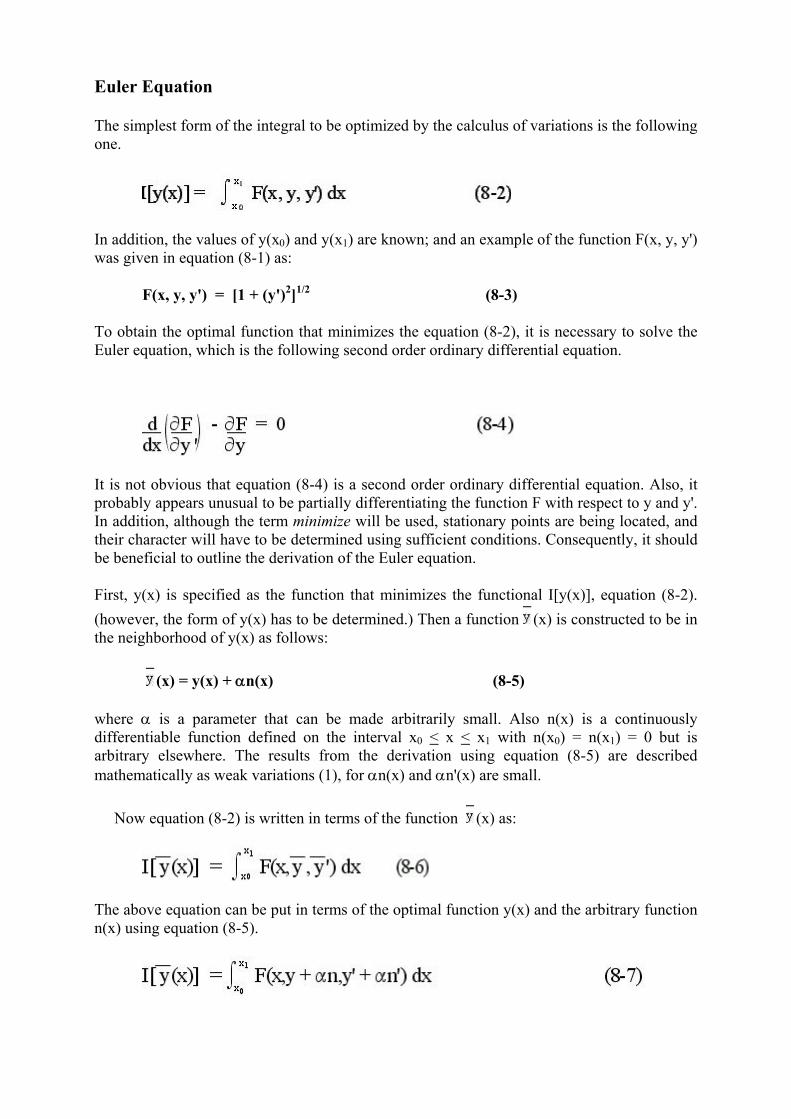
The simplest form of the integral to be optimized by the calculus of variations is the following one.

In addition, the values of y(x0) and y(x1) are known; and an example of the function F(x, y, y') was given in equation (8-1) as:

F(x, y, y') = [1 + (y')2]1/2 (8-3)

To obtain the optimal function that minimizes the equation (8-2), it is necessary to solve the Euler equation, which is the following second order ordinary differential equation.

It is not obvious that equation (8-4) is a second order ordinary differential equation. Also, it probably appears unusual to be partially differentiating the function F with respect to y and y'. In addition, although the term minimize will be used, stationary points are being located, and their character will have to be determined using sufficient conditions. Consequently, it should be beneficial to outline the derivation of the Euler equation.

First, y(x) is specified as the function that minimizes the functional I[y(x)], equation (8-2). (however, the form of y(x) has to be determined.) Then a function (x) is constructed to be in the neighborhood of y(x) as follows:

(x) = y(x) + αn(x) (8-5)

where α is a parameter that can be made arbitrarily small. Also n(x) is a continuously differentiable function defined on the interval x0 < x < x1 with n(x0) = n(x1) = 0 but is arbitrary elsewhere. The results from the derivation using equation (8-5) are described mathematically as weak variations (1), for αn(x) and αn'(x) are small.

Now equation (8-2) is written in terms of the function (x) as:

The above equation can be put in terms of the optimal function y(x) and the arbitrary function n(x) using equation (8-5).

The mathematical argument(3) is made that all of the possible functions lie in an arbitrarily small neighborhood of y because α can be made arbitrarily small. As such, the integral of equation (8-7) may be regarded as an ordinary function of α, Φ(α), because would specify the value of the integral knowing Φ(α = 0) at the minimum from y(x).

The minimum of Φ(α) is obtained by sitting the first derivative of Φ with respect to α equal to zero. The differentiation is indicated as:

Leibnitz' rule, equation (8-10), is required to differentiate the integral given in equation (8-9).

where x0 and x1 correspond to a1 and a2, and α corresponds to t.

The upper and lower limits, x0 and x1, are constants; and the following derivatives in the second and third terms on the right hand side of equation (8-10) are zero for this case.

Consequently, the order of integration and differentiation is interchanged, and equation (8-9) can be written as:

The integrand can be expanded as follows:

where dx/dα = 0, because x is treated as a constant in the mathematical argument of considering changes from curve to curve at constant x.

Substituting equation (8-13) into equation (8-12) gives:

The following results are needed:

Using equation (8-15), we can write equation (8-14) as:

An integration-by-parts will give a more convenient form for the term involving n' i.e.:

The first term on the right hand side is zero for n(xo) = n(x1) = 0. Combining the results from equation (8-17) with equation (8-16) gives:

At the optimum dΦ/dα = 0, and letting α → 0 has → y and '→ y'. Therefore, the above equation becomes:

To obtain the Euler equation the fundamental lemma of the calculus of variation is used. This lemma can be stated after Weinstock (3) as:

"If x0 and x1 (>x0) are fixed constants and G(x) is a particular continuous function in the interval x0 < x < x1 and if:

for every choice of the continuously differentiable function n(x) for which n(x0) = n(x1) = 0 then G(x) = 0 identically in the interval x0 < x < x1."

The proof of this lemma is by contradiction, and is given by Weinstock (3).

Applying this lemma to equation (8-18) gives the Euler equation.

This equation is a second order ordinary differential equation and has boundary conditions y(xo) and y(x1). The solution of this differential equation y(x) optimizes the integral I[y(x)].

A more convenient form of the Euler equation can be obtained by applying the chain rule to ∂F(x, y, y')/∂y'.

Substituting (equation 8-20) into equation (8-4) and rearranging gives a more familiar form for a second order ordinary differential equation.

A more convenient way to write this equation is:

The coefficients for the differential equation come from partially differentiating F.

A special case that sometimes occurs is to have F(y, y'), i.e., F is not a function of x. For this situation it can be shown that:

This equation may be integrated once to obtain a form of the Euler equation given below which can be a more convenient starting point for problem solving.

where the constant is evaluated using one of the boundary conditions.

At this point it should be noted that the necessary conditions of the classical theory of maxima and minima have been used to locate a stationary point. This point may be a minimum, maximum or saddle point. To determine its character, sufficient conditions must be

used; and these will be discussed subsequently. However, before that the following example is used to illustrate an application of the Euler equation.

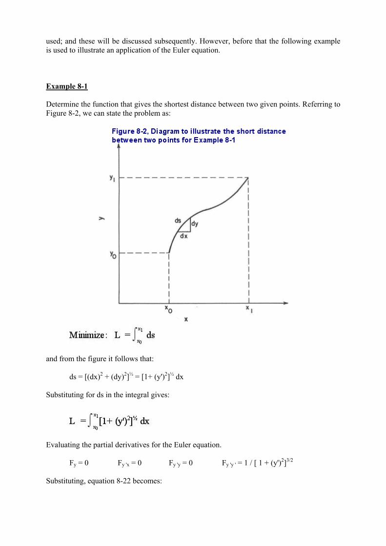
Example 8-1

Determine the function that gives the shortest distance between two given points. Referring to Figure 8-2, we can state the problem as:

and from the figure it follows that:

ds = [(dx)2 + (dy)2]½ = [1+ (y')2]½ dx

Substituting for ds in the integral gives:

Evaluating the partial derivatives for the Euler equation.

Fy = 0 Fy 'x = 0 Fy 'y = 0 Fy 'y ' = 1 / [ 1 + (y')2]3/2

Substituting, equation 8-22 becomes:

simplifying gives

Integrating the above equation twice gives:

y = c1 x + c2

This is the equation of a straight line; and the constants, c1 and c2, are evaluated from the boundary conditions.

Another classic problem of the calculus of variation as mentioned earlier is the Brachistochrone problem(10). The shape of the curve between two points is to be determined to minimize the time of a particle sliding along a wire without frictional resistance. The particle is acted upon only by gravitational forces as it travels between the two points. The approach to the solution is the same as for Example 8-1, and the integral for the time of travel, T, is given by Weinstock(3) as:

and the solution is in terms of the following parametric equations.

x = x0 + a[θ - sin(θ)] y = y0 + a[1 - cos(θ)] (8-26)

The details of the solution are given by Weinstock(3). The solution is the equations for a cycloid.

The method of obtaining the Euler equation is used almost directly to obtain the results for more detailed forms of the integrand of equation (8-2). The next section extends the results for more complex problems

More Complex Problems

In the procedure used to obtain the Euler equation, first a function was constructed to have the integral be a function of a single independent variable, i and then the classical theory of maxima and minima was applied to locate the stationary point. This same method is used for more complex problems which include more functions, e.g., y1, y2,..., yn; in higher order derivatives, e.g., y, y',..., y(n); and more than one independent variable, e.g., y(x1, x2). It is instructive to take these additional complications in steps. First, the case will be considered for one function y with higher order derivatives; and then this will be followed by the case of several functions with first derivatives, all for one independent variable. These results can then be combined for the case of several functions with higher order derivatives. The results will be a set of ordinary differential equations to be solved. Then further elaboration on the same ideas for the case of more than one independent variable will give a partial differential equation to be solved for the optimal function. Finally, any number of functions of varying

order of derivatives with several independent variables will require that a set of partial differential equations be solved for the optimal functions.

Functional with Higher Derivatives in the Integrand

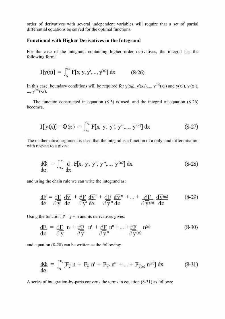
For the case of the integrand containing higher order derivatives, the integral has the following form:

In this case, boundary conditions will be required for y(x0), y'(x0),..., y(m)(x0) and y(x1), y'(x1), ..., y(m)(x1).

The function constructed in equation (8-5) is used, and the integral of equation (8-26) becomes.

The mathematical argument is used that the integral is a function of a only, and differentiation with respect to a gives:

and using the chain rule we can write the integrand as:

Using the function = y + n and its derivatives gives:

and equation (8-28) can be written as the following:

A series of integration-by-parts converts the terms in equation (8-31) as follows:

where equation (8-32) is the same as equation (8-17).

Equation (8-31) can be written as:

At the optimum a ® 0 to have ® y, ... , (m) y(m); and dF/da = 0 to give:

by employing the fundamental lemma of the calculus of variations.

This equation is normally written as follows and is called the Euler-Poisson equation.

This equation is an ordinary differential equation of order 2m and requires 2m boundary conditions. The following example illustrates its use in finding the optimal function.

Example 8-2(1)

Determine the optimum function that minimizes the integral in the following equation.

The Euler-Poisson equation for m = 2 is:

Evaluating the partial derivatives gives:

Substituting into the Euler- Poisson equation gives a fourth order ordinary differential equation.

The solution of this differential equation is:

y = c1e2x + c2e-2x + c3 cos 2x + c4 sin 2x

where the constants of integration are evaluated using the boundary conditions.

Functional with Several Functions in the Integrand

For the case of the integrand containing several functions, y1,y2,...,yp, the integral has the following form.

and boundary conditions on each of the functions are required, i.e., y1(x0), y1(x1), y2(x0), y2(x1), ..., yp(x0), yp(x1).

The function constructed in equation (8-5) is used, except in this case p functions are required.

1 = y1 + a1 n1 (8-38)

.

.

p = yp + ap np

with p parameters a1, a2,..., ap which can be made arbitrarily small. These equations are substituted into equation (8-37) and then the mathematical argument is used that the integral is a function of a1, a2,..., ap.

To locate the stationary point(s) of the integral, the first partial derivatives of F with respect to a1, a2,..., ap are set equal to zero. This gives the following set of p equations.

The chain rule is used with the function F, as previously to give:

Substituting into equation (8-40), we obtain an equation comparable to equation (8-16).

Integration by parts, letting ai ® 0 to have i ® yi and i' ® yi', and to have ¶F/¶ai = 0 gives the equation comparable to equation (8-18), i.e.:

Applying the fundamental lemma of the calculus of variations gives the following set of equations comparable to equation (8-4).

This is a set of Euler equations, and the following example illustrates the use of these equations to find the optimum set of functions.

Example 8-3(1)

Determine the optimum functions that determine the stationary points for the following integral.

The two Euler equations are:

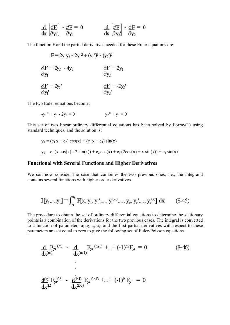
The function F and the partial derivatives needed for these Euler equations are:

The two Euler equations become:

-y1" + y2 - 2y1 = 0 y2" + y1 = 0

This set of two linear ordinary differential equations has been solved by Forray(1) using standard techniques, and the solution is:

y1 = (c1 x + c2) cos(x) + (c3 x + c4) sin(x)

y2 = c1 (x cos(x) - 2 sin(x)) + c2 cos(x) + c3 (2cos(x) + x sin(x)) + c4 sin(x)

Functional with Several Functions and Higher Derivatives

We can now consider the case that combines the two previous ones, i.e., the integrand contains several functions with higher order derivatives.

The procedure to obtain the set of ordinary differential equations to determine the stationary points is a combination of the derivations for the two previous cases. The integral is converted to a function of parameters a1,a2,..., ap, and the first partial derivatives with respect to these parameters are set equal to zero to give the following set of Euler-Poisson equations.

This is a set of p ordinary differential equations, and the order of each one is determined by the highest order derivative appearing in the integrand. The following example illustrates the use of these equations.

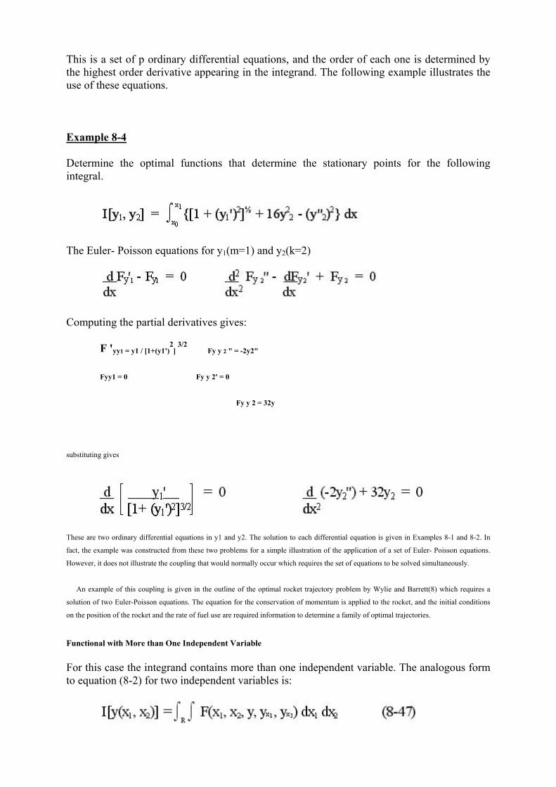
Example 8-4

Determine the optimal functions that determine the stationary points for the following integral.

The Euler- Poisson equations for y1(m=1) and y2(k=2)

Computing the partial derivatives gives:

F 'yy1 = y1 / [1+(y1')2

] 3/2

Fy y 2 " = -2y2"

Fyy1 = 0 Fy y 2' = 0

Fy y 2 = 32y

substituting gives

These are two ordinary differential equations in y1 and y2. The solution to each differential equation is given in Examples 8-1 and 8-2. In

fact, the example was constructed from these two problems for a simple illustration of the application of a set of Euler- Poisson equations.

However, it does not illustrate the coupling that would normally occur which requires the set of equations to be solved simultaneously.

An example of this coupling is given in the outline of the optimal rocket trajectory problem by Wylie and Barrett(8) which requires a

solution of two Euler-Poisson equations. The equation for the conservation of momentum is applied to the rocket, and the initial conditions

on the position of the rocket and the rate of fuel use are required information to determine a family of optimal trajectories.

Functional with More than One Independent Variable

For this case the integrand contains more than one independent variable. The analogous form to equation (8-2) for two independent variables is:

where the integral is integrated over the region R, and yx1 and yx2 indicate partial differentiation of y with respect to x1 and x2.

The procedure to obtain the differential equation to be solved for the optimal solution of equation (8-47) follows the mathematical

arguments used for the case of one independent variable. However, Green's theorem is required for the integration by parts, and the function

n(x1,x2) is zero on the surface of the region R. The function (x1,x2) is constructed from the optimal function y(x1,x2) and the arbitrary

function n(x1,x2) as:

(x1, x2) = y(x1, x2) + an(x1, x2) (8-48)

where is the parameter that can be made arbitrarily small.

Now the integral in equation (8-47) can be considered to be a function of a only, as was done in the previous mathematical arguments, i.e.:

I[ (x1 ,x2)] = I[y(x1, x2) + an(x1, x2)] = F(a) (8-49)

Then differentiating with respect to a gives an equation comparable to equation (8-12). The surface of the region R is a constant allowing the

interchange of the order of differentiation and integration.

Applying the chain rule as was done previously where F is not considered a funtion of x1 and x2 for changes from surface to surface, the

integrand becomes:

The

integral in equation (8-50) can be written in the following form using equation (8-50) and (8-51).

which is comparable to equation (8-16).

In this case the integration-by-parts is performed using Green's theorem in the plane which is:

This theorem is applied to the second two terms of equation (8-52) where f = n, G = ¶F/¶yxx1 and H = ¶F/¶yxx2 . An equation comparable to

equation (8-18) is obtained by allowing a ® 0 such that ® y, x1 ® yxx1 and x2 ® yxx2 ; and dF/da = 0 to have:

Again, it is argued using an extension of the fundamental lemma of the calculus of variations that if the integral is equal to zero, then the

term in the brackets is equal to zero because n(x1,x2) is arbitrary everywhere except on the boundaries where it is zero. The result is the

equation that corresponds to the Euler equation, equation (8-4).

Also, this equation can be expanded using the chain rule to give an equation that corresponds to equation (8-21) which is:

It can be seen that this is a second order partial differential equation in two independent variables. Appropriate boundary conditions at the

surface in terms of y and the first partial derivatives of y are required for a solution.

Prior to illustrating the use of equation (8-55), a general form is given from Burley(9) by the following equation for n independent variables

with only first partial derivatives in the integrand.

The derivation of this equation follows the one for two independent variables.

The following example illustrates an application of equation (8-55). Other applications are given by Forray(1) and Schechter(4).

Example 8-5(1)

The following equation describes the potential energy of a stretched membrane which is a minimum for small deflections. If A is the tension

per unit length and B is the external load, the optimum shape y(x1, x2) is determined by minimizing the integral.

Obtain the differential equation that is to be solved for the optimum shape.

The extension of the Euler Equation for this case of two independent variables was given by equation (8-55).

The integrand for F in the above equation is:

The following results are obtained from evaluating the partial derivatives.

Substituting into the equation and simplifying gives:

This is a second-order, elliptic partial differential equation. The solution requires boundary conditions that give the shape of the sides of the

membrane. The solution of the partial differential equation will be the shape of the membrane.

The text by Courant and Hilbert(5) gives the extension for higher order derivatives in the integrand. Also, that book gives solutions for a

number of problems including membrane shapes of rectangles and circles and is an excellent reference book on free and forced vibrations of

membranes. In the next section, the results for unconstrained problems are extended to those with constraints. The constraints can be of three

types for calculus of variations problems; and they are algebraic, integral, and differential equations

Constrained Variational Problems

Generally, there are two procedures used for solving variational problems that have constraints. These are the methods of direct substitution and Lagrange multipliers. In the method of direct substitution, the constraint equation is substituted into the integrand; and the problem is converted into an unconstrained problem as was done in Chapter II. In the method of Lagrange multipliers, the Lagrangian function is formed; and the unconstrained problem is solved using the appropriate forms of the Euler or Euler-Poisson equation. However, in some cases the Lagrange multiplier is a function of the independent variables and is not a constant. This is an added complication that was not encountered in Chapter II.

Algebraic Constraints

To illustrate the method of Lagrange multipliers, the simplest case with one algebraic equation will be used. The extension to more complicated cases are the same as that for analytical methods:

The Lagrangian function is formed as shown below.

L(x, y, y', λ) = F(x, y, y') + λ(x) G(x, y) (8-59)

The Lagrange multiplier λ is a function of the independent variable, x, and the unconstrained Euler equation is solved as given below.

along with the constraint equation G(x, y) = 0.

There is a Lagrange multiplier for each constraint equation when the Lagrangian function is formed. A derivation of the Lagrange multiplier method is given by Forray(1), and the following example illustrates the technique.

Example 8-6(8)

The classic example to illustrate this procedure is the problem of finding the path of a unit mass particle on a sphere from point (0,0,1) to point (0,0,-1) in time T, which minimizes the integral of the kinetic energy of the particle. The integral to be minimized and the constraint to be satisfied are:

The Langrangian function is:

L[x(t), y(t), z(t), λ(t)] = [(x')2 + (y')2 + (z')2]½ + λ(x2 + y2 + z2 - 1)

There are three optimal functions to be determined and the corresponding three Euler equations are:

Performing the partial differentiation of L, recognizing that [(x')2 + (y')2 + (z')2]½ = s' (an arc length which is a constant), and substituting into the Euler equations; three simple second order ordinary differential equations are obtained.

These can be integrated after some manipulations to give:

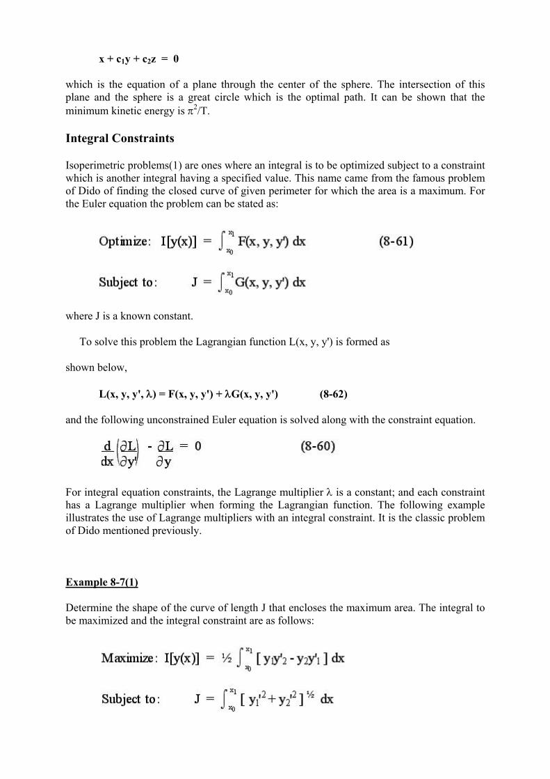
x + c1y + c2z = 0

which is the equation of a plane through the center of the sphere. The intersection of this plane and the sphere is a great circle which is the optimal path. It can be shown that the minimum kinetic energy is π2/T.

Integral Constraints

Isoperimetric problems(1) are ones where an integral is to be optimized subject to a constraint which is another integral having a specified value. This name came from the famous problem of Dido of finding the closed curve of given perimeter for which the area is a maximum. For the Euler equation the problem can be stated as:

where J is a known constant.

To solve this problem the Lagrangian function L(x, y, y') is formed as

shown below,

L(x, y, y', λ) = F(x, y, y') + λG(x, y, y') (8-62)

and the following unconstrained Euler equation is solved along with the constraint equation.

For integral equation constraints, the Lagrange multiplier λ is a constant; and each constraint has a Lagrange multiplier when forming the Lagrangian function. The following example illustrates the use of Lagrange multipliers with an integral constraint. It is the classic problem of Dido mentioned previously.

Example 8-7(1)

Determine the shape of the curve of length J that encloses the maximum area. The integral to be maximized and the integral constraint are as follows:

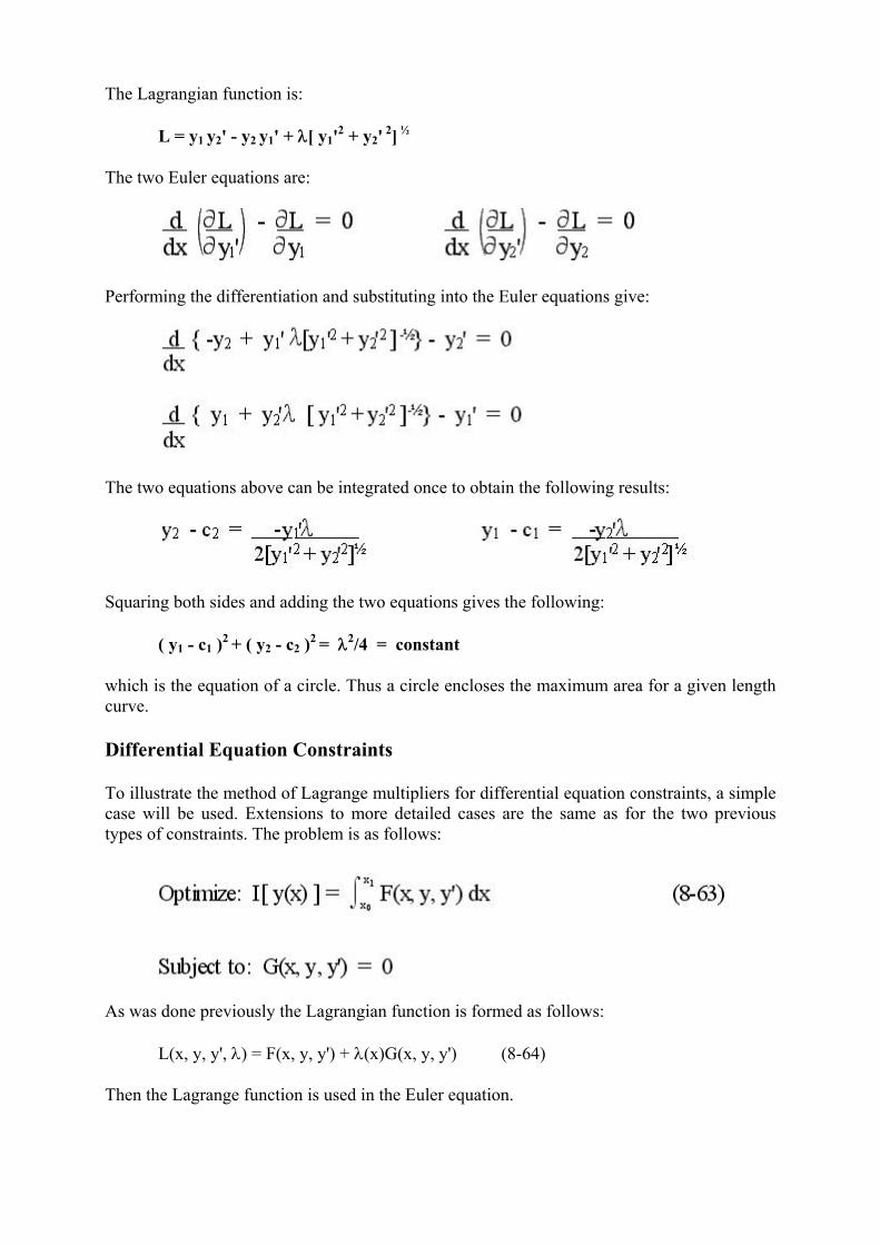
The Lagrangian function is:

L = y1 y2' - y2 y1' + λ[ y1'2 + y2' 2] ½

The two Euler equations are:

Performing the differentiation and substituting into the Euler equations give:

The two equations above can be integrated once to obtain the following results:

Squaring both sides and adding the two equations gives the following:

( y1 - c1 )2 + ( y2 - c2 )2 = λ2/4 = constant

which is the equation of a circle. Thus a circle encloses the maximum area for a given length curve.

Differential Equation Constraints

To illustrate the method of Lagrange multipliers for differential equation constraints, a simple case will be used. Extensions to more detailed cases are the same as for the two previous types of constraints. The problem is as follows:

As was done previously the Lagrangian function is formed as follows:

L(x, y, y', λ) = F(x, y, y') + λ(x)G(x, y, y') (8-64)

Then the Lagrange function is used in the Euler equation.

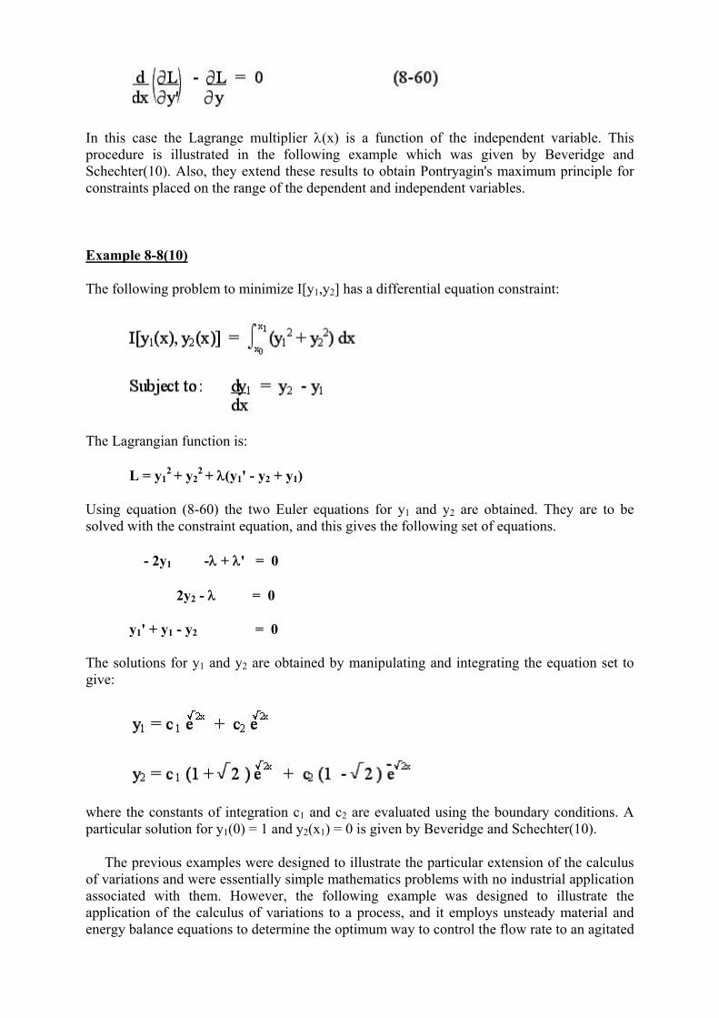
In this case the Lagrange multiplier λ(x) is a function of the independent variable. This procedure is illustrated in the following example which was given by Beveridge and Schechter(10). Also, they extend these results to obtain Pontryagin's maximum principle for constraints placed on the range of the dependent and independent variables.

Example 8-8(10)

The following problem to minimize I[y1,y2] has a differential equation constraint:

The Lagrangian function is:

L = y12 + y2

2 + λ(y1' - y2 + y1)

Using equation (8-60) the two Euler equations for y1 and y2 are obtained. They are to be solved with the constraint equation, and this gives the following set of equations.

- 2y1 -λ + λ' = 0

2y2 - λ = 0

y1' + y1 - y2 = 0

The solutions for y1 and y2 are obtained by manipulating and integrating the equation set to give:

where the constants of integration c1 and c2 are evaluated using the boundary conditions. A particular solution for y1(0) = 1 and y2(x1) = 0 is given by Beveridge and Schechter(10).

The previous examples were designed to illustrate the particular extension of the calculus of variations and were essentially simple mathematics problems with no industrial application associated with them. However, the following example was designed to illustrate the application of the calculus of variations to a process, and it employs unsteady material and energy balance equations to determine the optimum way to control the flow rate to an agitated

tank. Although the example is relatively simple, it illustrates economic model and process constraints for a dynamic system; and an optimal control function is developed.

Example 8-9(11)

An agitated tank contains W pounds of water at 32°F. It is desired to raise the temperature of the water in the tank to 104°F in (2.0)½ hours by feeding water at a rate of W lb. per hour. The tank is completely filled with water, and the overflow water at T2(t) is equal to the input flow rate at T1(t). The average residence time of water in the tank is one hour, and the tank is perfectly mixed. The temperature of the inlet can be adjusted as a function of time by an electric heater in the feed pipe which is connected to a variable voltage transformer. The sensible heat accompanying water flowing into and out of the tank during the process must be considered lost. Therefore, it is, desired to minimize the integral of the sum of squares of the difference between the temperatures, T1(t) and T2(t), and the reference temperature, 32°F. This economic model is given by the following equation.

An unsteady-state energy balance on the water in the tank at time t gives the following equation relating the temperatures T1(t), T2(t) and the system parameters.

For water the heat capacity, Cp, is equal to 1.0 BTU/lb°F, and this equation simplifies to the following form:

The calculus of variations problem can now be formulated as:

with T1(0) = T2(0) = 32°F, and T2 (√2) = 104°F as boundary conditions.

Two optimal functions are determined, and the solution of two Euler equations are required using equation (8-60). The Lagrangian function is:

L[T1(t),T2(t), λ(t)] = (T1 - 32)2 + (T2 - 32)2 + λ(t)[T2' - T1 + T2]

and the Euler equations are:

The results of performing the differentiation are:

Substituting into the Euler equations gives the following set of equations.

The third equation is the constraint, and these equations are solved for T1(t) and T2(t). The set has two ordinary differential equations and one algebraic equation. Manipulating and solving this set for one equation in terms of T2(t) gives:

T2" - 2T2 = - 64

With the boundary conditions of T2(0) = 32 and T2 (√2) = 104, the solution to the differential equation is:

where 9.91 = 72/(e2 - e-2). The constraint is used to obtain the entering water temperature as a function of time, and substituting in the solution for T2(t) gives:

The solutions for the optimal functions, T1(t) and T2(t) are tabulated and plotted in Figure 8-3. As shown in the figure the warm water temperature increases to 209°F for the water temperature in the tank to reach 104°F in √2 hours.

Closure

Some of the important results from the chapter are summarized in an abbreviated form in Table 8-1. First, a set of Euler equations is shown in the table to be solved when the integrand contains several optimal functions and their first derivatives. Corresponding boundary conditions are required on each of these Euler equations which are second order ordinary differential equations. Next in the table is the integral that has higher order derivatives in the integrand. For this case the Euler-Poisson equation has to be solved, and it is of order 2m, where m is the order of the highest derivative in the integrand. Also appropriate boundary conditions on y and its derivatives at x0 and x1 are required to obtain the particular solution of the differential equation. A combination of these two cases is given in the table where a set of Euler-Poisson equations is solved for the optimum functions.

When the optimal function involves more than one independent variable a partial differential equation has to be solved, and the table shows the case for two independent variables, a second order partial differential equation. Equation (8-57) gives the comparable equation for n independent variables. However, the results given in the table and the chapter are only for an optimal function with first partial derivatives in the integrand. Results comparable to the Euler-Poisson equation with higher order derivatives are available in Weinstock(3).

When constraints are involved the Lagrange function is formed as shown in the table. This gives an unconstrained problem that can be solved by the Euler and/or Euler Poisson equation, along with the constraint equations.

The purpose of the chapter was to give some of the key results of the calculus of variations, and to emphasize the similarities and differences between finding an optimal function and an optimal point. Consequently, it was necessary to select the methods given here from some equally important methods that were omitted. Two of these are the concept of a variation and the use of the second variation for the sufficient conditions to determine if the function was actually a maximum or minimum. These are discussed by Courant and Hilbert(5) along with the problem of the existence of a solution. Also, most texts discuss the moving (or natural) boundary problem where one or both of the limits on the integral to be optimized can be a function of the independent variable. This leads to extensions of the Brachistochrone problem and Forray's discussion(1) is recommended. With the background of this chapter, extension to Hamilton's principle follows, and is typically the next topic presented on the subject. Also, this material leads to extensions that include Pontryagin's maximum principle, Sturm-Liouville problems, and application in optics, dynamics of particles, vibrations, elasticity, and quantum mechanics.

The calculus of variations can be used to solve transport phenomena problems, i.e., obtain solutions to the partial differential equations representing the conservation of mass, momentum and energy of a system. In this approach the partial differential equations are converted to the corresponding integral to be optimized from the calculus of variations. Then approximate methods of integration are used to find the minimum of the integral, and this yields the concentration, temperature and/or velocity profiles required for the solution of the original differential equations. This approach is described by Schechter(4) in some detail.

Again the purpose of the chapter was to introduce the topic of finding the optimal function. The references at the end of the chapter are recommended for further information; they include the texts by Fan(12) and Fan and Wang(13) on the maximum principle and Kirk(14) among others (7,15,16) on optimal control.

References

1. Forray, M. J., Variational Calculus in Science and Engineering, McGraw-Hill Book Company, New York (1968).

2. Ewing, G. M. Calculus of Variations with Applications, W.W. Norton Co. Inc, New York (1969).

3. Weinstock, Robt. Calculus of Variations, McGraw-Hill Book Company, New York (1952).

4. Schechter, R. S. The Variational Method in Engineering, McGraw-Hill Book Company, New York (1967).

5. Courant, R. and D. Hilbert, Methods of Mathematical Physics, Vol. I, John Wiley and Sons, Inc., New York (1953).

6. Sagan, Hans Introduction to the Calculus of Variations, McGraw Hill Book Co., New York (1969).

7. M.M. Denn, Optimization by Variational Methods, McGraw-Hill Book Company, New York (1970).

8. Wylie, C. R. and L. C. Barrett, Advanced Engineering Mathematics 5th Ed., McGraw-Hill Book Company, New York (1982).

9. Burley, D. M., Studies in Optimization, John Wiley and Sons, Inc., New York (1974).

10. Beveridge, G. S. G. and R. S. Schechter, Optimization: Theory and Practice, McGraw-Hill Book Company, New York (1970).

11. Fan, L.T., E.S. Lee, and L.E. Erickson, Proc. of the Mid-Am. States Univ. Assoc. Conf. on Modern Optimization Techniques and their Application in Engineering Design, Part I, Kansas State University, Manhattan, Kansas (Dec.19-22,1966).

12. L.T. Fan, The Continuous Maximum Principle, John Wiley and Sons Inc., New York (1966).

13. L.T. Fan and C.S. Wang, The Discrete Maximum Principal, John Wiley and Sons Inc., New York (1964).

14. Kirk, D.E. Optimal Control Theory, An Introduction. Prentice Hall, Inc., Englewood Clifffs, New Jersey (1970).

15. Miele, A. , Optimization Techniques with Applications to Aerospace Systems, Ed., G. Leitman, Ch.4, Academic Press, New York (1962).

16. Connors, M. M. and D. Teichroew, Optimal Control of Dynamic Operations Research Models, International Textbook Inc., Scranton, Pennsylvania (1967)

Problems

8-1(16). A product is being produced at a steady rate of P0 pounds per hour. It is necessary to change the production rate to P1 pounds per hour and minimize the cost resulting from raw material lost to off-specification product and overtime wages during the transition period. This is modeled by the following cost function.

C(t) = c1 P'2 + c2 tP'

where c1 and c2 are cost coefficients and P'= dP/dt. The total cost for the change in the production schedule is given by:

where Po = P(to) and P1 = P(t1) are known.

Determine the optimum way the production rate P(t) is to be changed to minimize the total cost.

Solution

The Euler equation is solved for P(t) which minimizes CT.

C(t) = C1P'2 + C2tP'

The Euler equation is:

Substituting gives:

Integrating twice gives:

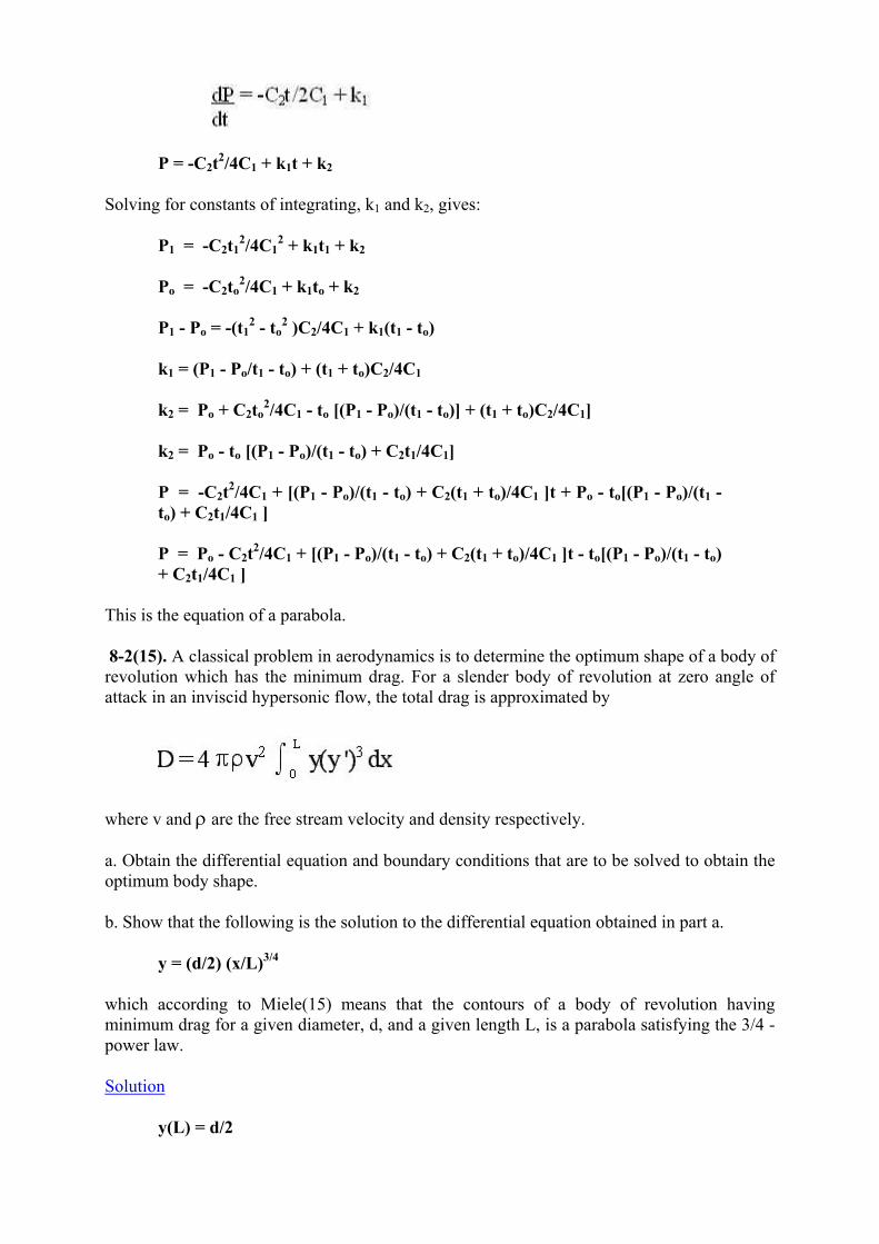
P = -C2t2/4C1 + k1t + k2

Solving for constants of integrating, k1 and k2, gives:

P1 = -C2t12/4C1

2 + k1t1 + k2

Po = -C2to2/4C1 + k1to + k2

P1 - Po = -(t12 - to

2 )C2/4C1 + k1(t1 - to)

k1 = (P1 - Po/t1 - to) + (t1 + to)C2/4C1

k2 = Po + C2to2/4C1 - to [(P1 - Po)/(t1 - to)] + (t1 + to)C2/4C1]

k2 = Po - to [(P1 - Po)/(t1 - to) + C2t1/4C1]

P = -C2t2/4C1 + [(P1 - Po)/(t1 - to) + C2(t1 + to)/4C1 ]t + Po - to[(P1 - Po)/(t1 - to) + C2t1/4C1 ]

P = Po - C2t2/4C1 + [(P1 - Po)/(t1 - to) + C2(t1 + to)/4C1 ]t - to[(P1 - Po)/(t1 - to) + C2t1/4C1 ]

This is the equation of a parabola.

8-2(15). A classical problem in aerodynamics is to determine the optimum shape of a body of revolution which has the minimum drag. For a slender body of revolution at zero angle of attack in an inviscid hypersonic flow, the total drag is approximated by

where v and ρ are the free stream velocity and density respectively.

a. Obtain the differential equation and boundary conditions that are to be solved to obtain the optimum body shape.

b. Show that the following is the solution to the differential equation obtained in part a.

y = (d/2) (x/L)3/4

which according to Miele(15) means that the contours of a body of revolution having minimum drag for a given diameter, d, and a given length L, is a parabola satisfying the 3/4 - power law.

Solution

y(L) = d/2

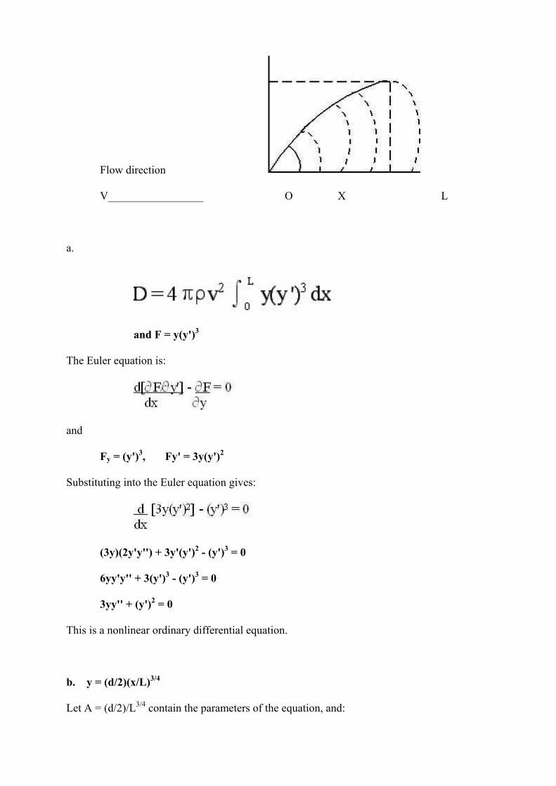
Flow direction

V_________________ O X L

a.

and F = y(y')3

The Euler equation is:

and

Fy = (y')3, Fy' = 3y(y')2

Substituting into the Euler equation gives:

(3y)(2y'y'') + 3y'(y')2 - (y')3 = 0

6yy'y'' + 3(y')3 - (y')3 = 0

3yy'' + (y')2 = 0

This is a nonlinear ordinary differential equation.

b. y = (d/2)(x/L)3/4

Let A = (d/2)/L3/4 contain the parameters of the equation, and:

y = Ax3/4

y' = 3/4 Ax -1/4

y" = -3/16 Ax -5/4

Substituting the above into the differential equation in part a gives:

3(Ax3/4)(-3/16 Ax -5/4) + (3/4 Ax -1/4)2 = 0

-9/16 A2x -1/2 + 9/16 A2x -1/2 = 0

Thus, this equation is a solution to the differential equation.

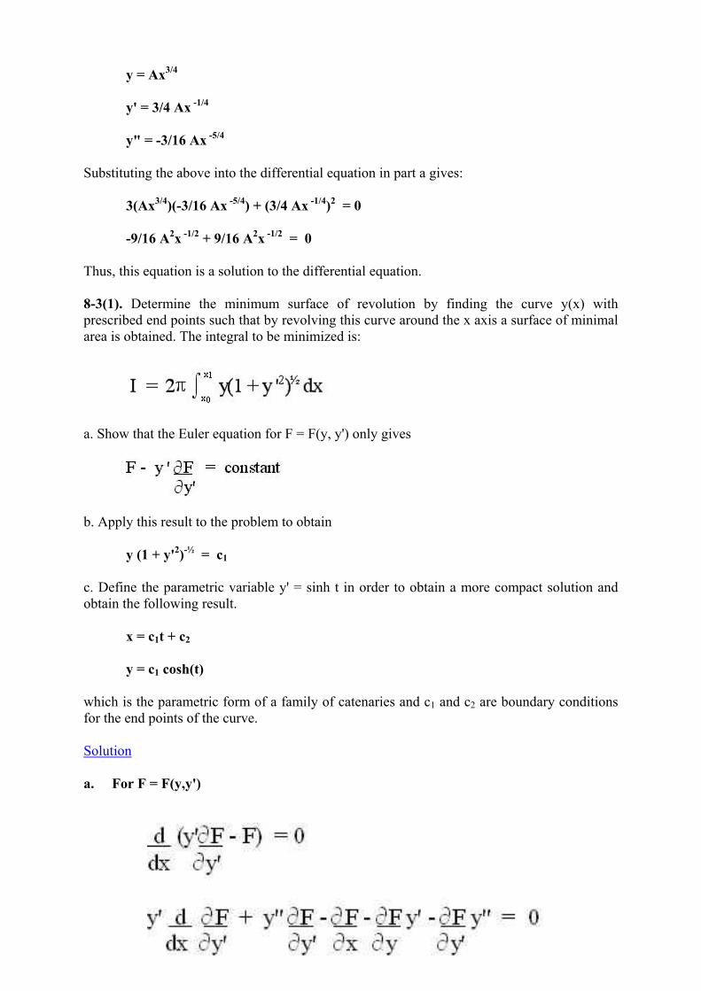
8-3(1). Determine the minimum surface of revolution by finding the curve y(x) with prescribed end points such that by revolving this curve around the x axis a surface of minimal area is obtained. The integral to be minimized is:

a. Show that the Euler equation for F = F(y, y') only gives

b. Apply this result to the problem to obtain

y (1 + y'2)-½ = c1

c. Define the parametric variable y' = sinh t in order to obtain a more compact solution and obtain the following result.

x = c1t + c2

y = c1 cosh(t)

which is the parametric form of a family of catenaries and c1 and c2 are boundary conditions for the end points of the curve.

Solution

a. For F = F(y,y')

b.

Let F = y 1 + (y')2

Using Euler Equation

Simplifying gives:

y[1 + (y')2]-½ = C1

c. Given y' = sinh(t), then integrating gives:

y = C1 cosh t

Then using the above gives:

dx = dy/y' = C1 sinh(t) dt/sinh(t) = C1 dt

Integrating the above gives:

x = C1t + C2

and y1 = C1 cosh t

This is the parametric form of a family of catenaries, and the constants C1 and C2 are determined from end points of the curves.

8-4(9). Find the shape at equilibrium of a chain of length, L, which hangs from two points at the same level. The potential energy, E, of the chain is given by the following equation:

and is subject to the specified total length L by the following equation.

with boundary conditions of y(x0) = y(x1) = 0. To obtain the equilibrium shape of the chain, it is necessary to minimize the energy subject to the length restriction. Show that the following differential equation is obtained from the Euler equation.

y' = [k2 (y + λ)2 - 1]½

Make the substitution k(y + λ) = coshθ ,and obtain the solution given below.

cosh k(x + α) = k (y + λ)

This curve is the catenary, and the constants k, α, λ can be obtained from the boundary conditions and the constraint on L.

Solution

Using the Lagrange multiplier method, the following unconstrained extremum is obtained.

F = (y + λ)[1 + (y')2]½

C = y' ∂F/∂y' - F

(y')2 = C2(y + λ)2 - 1

y' = [C2(y + λ)2 - 1]½

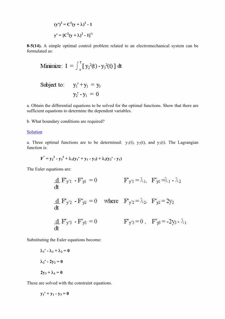
8-5(14). A simple optimal control problem related to an electromechanical system can be formulated as:

a. Obtain the differential equations to be solved for the optimal functions. Show that there are sufficient equations to determine the dependent variables.

b. What boundary conditions are required?

Solution

a. Three optimal functions are to be determined: y1(t), y2(t), and y3(t). The Lagrangian function is:

F* = y22 - y3

2 + λ1(y1' + y1 - y3) + λ2(y2' - y1)

The Euler equations are:

Substituting the Euler equations become:

λ1' - λ1 + λ2 = 0

λ2' - 2y2 = 0

2y3 + λ1 = 0

These are solved with the constraint equations.

y1' + y1 - y3 = 0

y2' - y1 = 0

There are five differential equations and five dependent variables: y1(t), y2(t), y3(t), 1(t) and 2(t) which area function of t.

b. Boundary conditions are required at t=0 and t=T as shown below.

y1(0) = y10 y1(T) = y1T

y2(0) = y20 y2(T) = y2T

y3(0) = y30 y3(T) = y3T

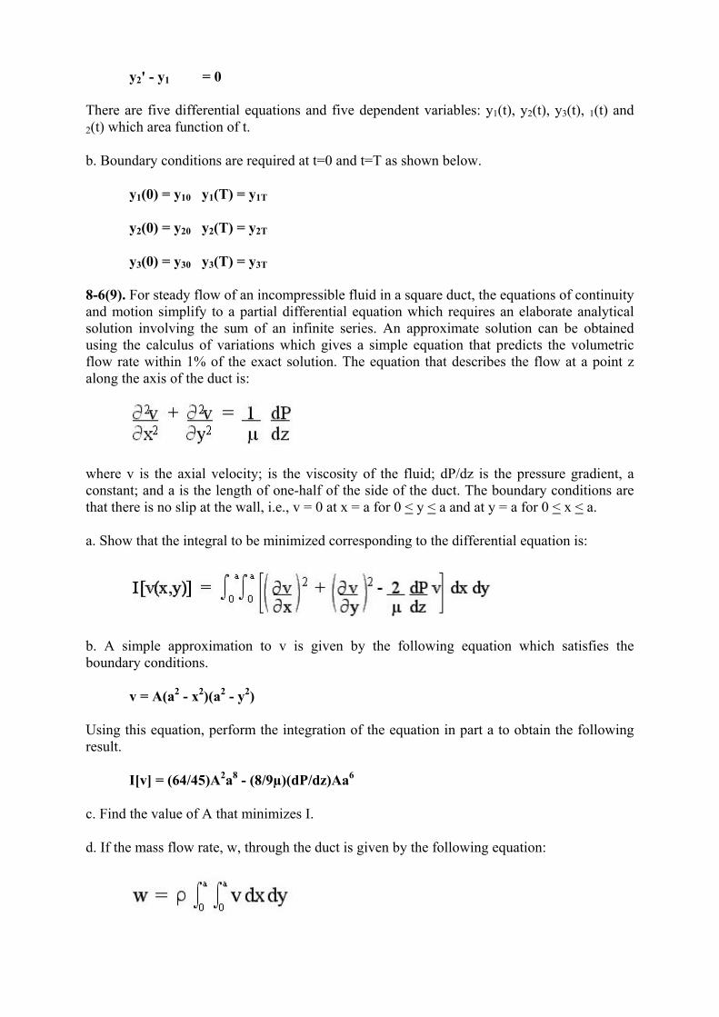
8-6(9). For steady flow of an incompressible fluid in a square duct, the equations of continuity and motion simplify to a partial differential equation which requires an elaborate analytical solution involving the sum of an infinite series. An approximate solution can be obtained using the calculus of variations which gives a simple equation that predicts the volumetric flow rate within 1% of the exact solution. The equation that describes the flow at a point z along the axis of the duct is:

where v is the axial velocity; is the viscosity of the fluid; dP/dz is the pressure gradient, a constant; and a is the length of one-half of the side of the duct. The boundary conditions are that there is no slip at the wall, i.e., v = 0 at x = a for 0 < y < a and at y = a for 0 < x < a.

a. Show that the integral to be minimized corresponding to the differential equation is:

b. A simple approximation to v is given by the following equation which satisfies the boundary conditions.

v = A(a2 - x2)(a2 - y2)

Using this equation, perform the integration of the equation in part a to obtain the following result.

I[v] = (64/45)A2a8 - (8/9µ)(dP/dz)Aa6

c. Find the value of A that minimizes I.

d. If the mass flow rate, w, through the duct is given by the following equation:

show that the following result is obtained:

w = 0.556 ρ(dP/dz)a4 / µ

The analytical solution has the same form, but the coefficient is 0.560. Thus the approximate solution is within 1% of the exact solution.

Solution

a. For

The extension of Euler equation for this case of two independent variables was given by equation (8-55).

This equation can be written as:

The integrand for F in the above equation is:

F = (∂v/∂x)2 + (∂v/∂y)2 - (2/µ)(dP/dz) v

The partial derivatives appearing in the Euler equation are:

∂F/∂vx = 2(∂v/∂x) , ∂F/∂vy = 2(∂v/∂y)

∂F/∂v = - (2/µ)(dP/dz)

Substituting the above expressions into the Euler equation gives:

This is the differential equation required.

b.

v = A(a2 - x2)(a2 - y2)

vx = A(-2x)(a2 - y2)

vx2 = 4A2x2(a4 - 2a2y2 + y4)

vy = A(-2y)(a2 - x2)

vy2 = 4A2y2(a4 - 2a2x2 + x4)

Performing the integration in steps as follows, gives:

= 4A2[8a8/45]

Similarly:

= - (2/µ)(dP/dz) A(4a6/9) = - (8a6A/9µ)(dP/dz)

I[v] = (64/45) A2a8 - (8a6A/9µ)(dP/dz)

c.

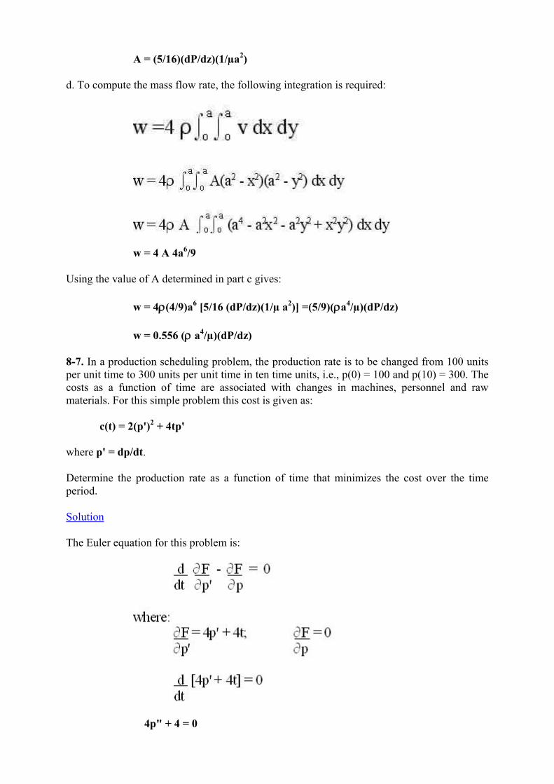
A = (5/16)(dP/dz)(1/µa2)

d. To compute the mass flow rate, the following integration is required:

w = 4 A 4a6/9

Using the value of A determined in part c gives:

w = 4ρ(4/9)a6 [5/16 (dP/dz)(1/µ a2)] =(5/9)(ρa4/µ)(dP/dz)

w = 0.556 (ρ a4/µ)(dP/dz)

8-7. In a production scheduling problem, the production rate is to be changed from 100 units per unit time to 300 units per unit time in ten time units, i.e., p(0) = 100 and p(10) = 300. The costs as a function of time are associated with changes in machines, personnel and raw materials. For this simple problem this cost is given as:

c(t) = 2(p')2 + 4tp'

where p' = dp/dt.

Determine the production rate as a function of time that minimizes the cost over the time period.

Solution

The Euler equation for this problem is:

4p" + 4 = 0

p" = -1

Integrating this simple second-order ordinary differential equation gives:

p' = -t + C1

p = -t2/2 + C1t + C2

Solving for C1 and C2 with the boundary conditions give:

100 = 0 + C1(0) + C2 and C2 = 100

300 = -100/2 + 10C1 + C2 and C1 = 25

C1 = 25

Substituting, the particular solution is:

p = -t2/2 + 25t + 100

8-8(1). Determine the deflection in an uniformly-loaded, cantilever beam, y(x), where y is the deflection as a function of distance down the beam from the wall (x=0) to the end of the beam (x = L). The total potential energy of the system to be minimized is given by:

where E is the bending rigidity and q is the load. The boundary conditions at the wall end are y(0) = y'(0) = 0 and at the supported end of y'''(L) = y"(L) = 0.

Solution

The Euler-Poisson equation for m = 2 is:

For this problem, the integrand is:

Performing the partial differentiation gives:

Substituting into the Euler-Poisson equation gives:

The boundary conditions for this fourth-order ordinary differential are:

y(0) = 0 y"(L) = 0

y'(0) = 0 y"(L) = 0

Integrating the differential equation one time gives:

d3y/dx3 = q/E x + C1

Using y'''(L) = 0, C1 can be evaluated and is:

C1 = -qL/E

The differential equation becomes:

d3y/dx3 = qx/E - qL/E

Integrating again gives:

d2y/dx2 = (q/E)(x2/2) - (q/E)(Lx) + C2

Using y"(L) = 0, C2 can be evaluated and is:

C2 = qL2/2E

The differential equation becomes:

d2y/dx2 = (q/E)(x2/2) - (q/E)(Lx2/2) + qL2/2E

Integrating again gives:

dy/dx = (q/E)(x3/6) - (q/E)Lx2/2 + (qL2/2E)(x) + C3

Using y'(0) = 0, C3 = 0. This integrating again gives:

y = (q/E)x4/24 - qLx3/6E + (qL2/2E)(x2/2) + C4

Using y(0) = 0, C4 = 0; and the solution is:

y = (q/E)(x4/24) - (qL/E)(x3/6) + (qL2/E)(x2/4)

or

y = q/2E [ (x4/12) - (Lx3/3) + (L2x2/2)]