characterisation of fracture network realisations for … · characterisation of fracture network...

Proceedings World Geothermal Congress 2015

Melbourne, Australia, 19-25 April 2015

1

Characterisation of Fracture Network Realisations for Geothermal Reservoir Flow

Modelling

Marc K. Elmouttie, Brett Poulsen and Greg Krahenbuhl

CSIRO Earth Science and Resource Engineering

[email protected]

Keywords: Discrete fracture network modeling, Monte Carlo simulation, uncertainty quantification

ABSTRACT

Characterisation of fractured reservoirs is required for prediction of the economic viability of geothermal projects. However,

accurate characterisation is often not possible mainly because of the uncertainties associated with fracture properties such as

location, size, orientation and aperture. Modelling of fluid flow in geothermal reservoirs often requires explicit representation of the

fracture network as only a minority of the fractures may be responsible for the majority of the flow. To account for the uncertainty,

stochastic methods are used and multiple fracture network realisations are generated.

Given the computation time associated with performing a fluid flow analysis, only a subset of these fracture network realisations

can be analysed. We have investigated the use of fast-to-compute geometry based metrics to characterise individual fracture

network realisations prior to selection of a sub-set for explicit fluid flow analyses, the goal being to select realisations that

accurately represent both conservative and aggressive scenarios. To assess the success of the metrics, we used a fluid flow solver

utilising a pipe network generator to represent the fracture networks as connected 1-dimensional flow elements. We find that the

success of such metrics depends on the complexity of the fracture network.

1. INTRODUCTION

The goal of any rock mass modelling is to capture the salient features of the rock for the purposes of the analysis to be undertaken.

Heterogeneity of the rock mass results in both model uncertainty and stochastic uncertainty. The former results from our limited

understanding of the geology, hydrogeology, discontinuities and rock matrix present in the field. The latter is present even if our

understanding is accurate because many of the properties of interest (e.g. fracture diameter and aperture) can only practically be

considered to be stochastic variables.

The effective fracture network permeability of a geothermal reservoir is clearly subject to both types of uncertainties. Stochastic

modelling approaches can be used to quantify the uncertainty in estimation of reservoir properties and performance however

computational methods must be efficient enough to support timely analysis and ideally allow the engineer to use an iterative

approach to refine and confirm an understanding of the reservoir. The work described in this paper attempts to at least partially

address this requirement by providing a method to efficiently quantify the uncertainty associated with geothermal reservoir flow

modelling.

Modern computing facilities mean that modelling of complex physics associated with geothermal and enhanced geothermal

systems is now possible. Sophisticated physics, coupled processes, complex geologies and stochastic processes can all be evaluated

given enough computing time. The parameters associated with the modelling process can be divided into 3 spaces: model

size/scale, physics complexity and representation of uncertainty. The latter refers to both model uncertainty and stochastic

uncertainty. Figure 1 shows a schematic representation of these parameters.

Figure 1 The parameters associated with the modelling process

Elmouttie, Poulsen and Krahenbuhl

2

Very often, the representation of uncertainty is neglected in an attempt to model the most sophisticated physics and detailed

geometry possible. However, the heterogeneity of the rock mass is often crucial in many areas of rock mechanics, including slope

stability, reservoir characterisation, blasting and rock processing. Explicit representation of the rock mass heterogeneity facilitates

the representation of uncertainty.

For understanding fluid flow through fractured rock, the heterogeneity of the fracture network needs to be captured accurately.

There are alternate ways to represent this and the two fundamentally different approaches can be labelled stochastic continuum

methods using effective porous medium (EPM) and stochastic discrete methods using discrete fracture networks (DFN).

In EPM modelling, the simulation volume is discretised into gridded blocks and the properties of the rock mass in each block are

averaged out. Most reservoir modelling of fractured rock masses use this approach but implement what is known as a dual-porosity

model (i.e. dual referring to the fracture network versus the rock matrix). This modelling is valid for rock masses with high fracture

frequencies and well connected networks so that the fracture properties can be averaged out over a grid block. Clearly, this

approach is of limited use for reservoirs where the flow occurs predominantly through a small number of fractures in the network.

In DFN modelling, fractures are individually represented in the model allowing the simulation process to account for the individual

fracture properties (orientation, size, location, aperture etc) and ensemble properties (density, connectivity etc). However, explicit

representation of fractures and rock mass defects imposes very significant computational costs in both processing time and memory

consumption. This is especially true for complex DFN modelling where hundreds of thousands of individual fractures may be

required. Moreover, for stochastic modelling, hundreds or thousands of DFN realisations may need to be generated and used in the

modelling process to determine confidence intervals for model predictions.

In practice, the computer codes capable of numerically modelling the fluid flow through even a single DFN realisation for simple

scenarios is computationally expensive and therefore it is only practical to numerically model a small subset of DFN realisations.

The flow response of individual DFN realisations can differ markedly so guidance is required in the choice of which realisations to

use in the modelling process. Figure 2 shows an analysis of fracture network connectivity associated with two realisations of a

geothermal reservoir. Clearly some apriori knowledge of the properties of individual realisations as they pertain to fluid flow

through the reservoir would assist the choice of realisations for numerical modelling.

Figure 2 Example of two different predictions of fracture network connectivity associated with two realisations of a

geothermal reservoir. Fractures with black outline indicate the conducting part of the network.

These two modelling approaches with their specific advantages need not be exclusive if the anisotropic fluid flow properties

required as an input property for the EPM are estimated based on DFN modelling. This approach is further optimised if an estimate

can be made of the realisations place in the parameter space, for example if the overall permeability is at the 50th, 70th or 90th

percentile of the distribution of realisations.

The aim of this paper is to address the computational issues by providing techniques to identify which DFN realisations should be

selected for modelling to accurately characterise the confidence intervals. By doing so, the number of numerical simulations can be

drastically reduced. DFN based analysis for reservoir modelling, predominantly in the hydrocarbon industry, has a long history.

The analysis of fluid flow properties of fractured reservoirs is based on connectivity analysis associated with percolation theory of

porous media (Berkowitz 1995). The concept of the percolation threshold can be adapted to fracture networks as follows.

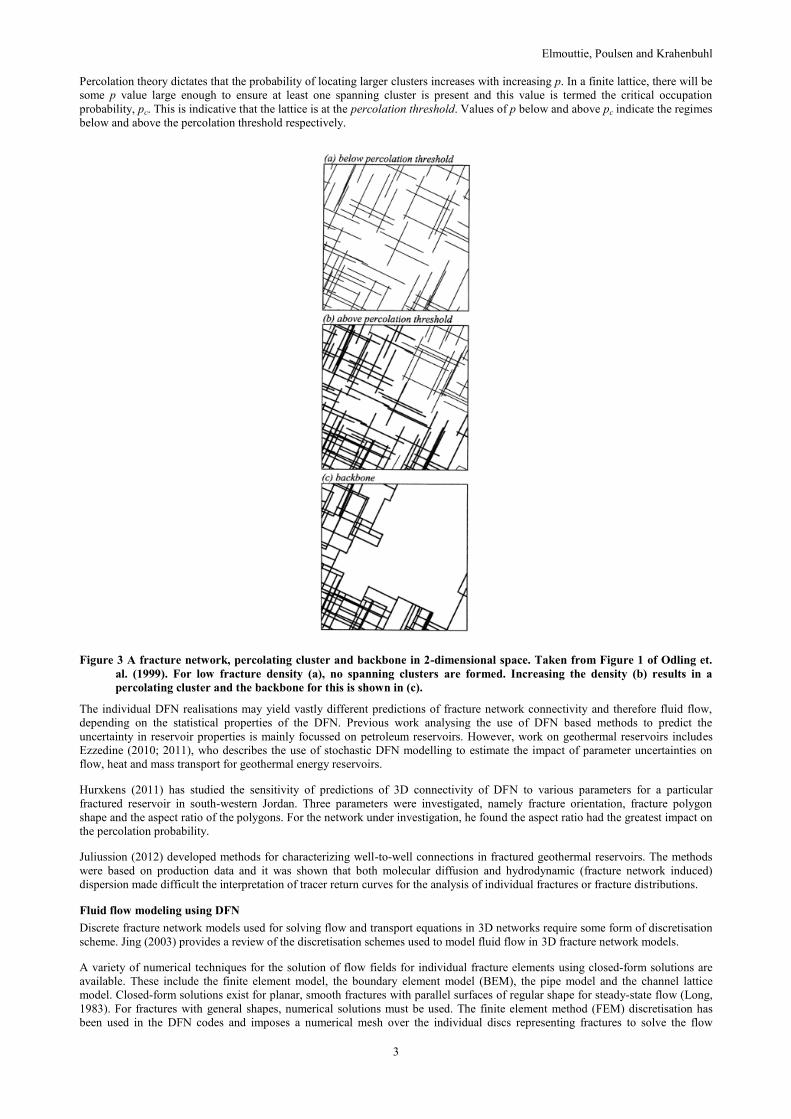
Consider a lattice with clusters - groups of interconnected bonds or sites. For a finite lattice, the probability that a site belongs to a

cluster that connects opposing faces of the lattice (percolating or spanning cluster- see Figure 3) is defined as p. There is also the

concept of the backbone which indicates the conducting part of the percolating cluster, or in other words, the subset of fractures

required to maintain the flow through the cluster (Figure 3c). Note that the backbone need not include all the fractures belonging to

the percolating cluster. Graph theory is used to identify fractures belonging to the backbone, and fractures which link to the

backbone but do not provide connectivity back to it will be marked as not part of the backbone. Note that the definition of a

backbone in 2D is much more trivial than in 3D. For example, Priest (1993, chapter 6) presents a discussion of the removal of

unused fractions of fractures from the backbone, a process that makes sense in 2D but not in 3D were partially intersecting fractures

are possible. The connectivity of a synthetic fracture network is also sensitive to the assumptions used in the generation process.

For example, Bonneau et. al. (2013) have shown that the planar fracture assumption can lead to a significant under-estimation of

connectivity.


3

Percolation theory dictates that the probability of locating larger clusters increases with increasing p. In a finite lattice, there will be

some p value large enough to ensure at least one spanning cluster is present and this value is termed the critical occupation

probability, pc. This is indicative that the lattice is at the percolation threshold. Values of p below and above pc indicate the regimes

below and above the percolation threshold respectively.

Figure 3 A fracture network, percolating cluster and backbone in 2-dimensional space. Taken from Figure 1 of Odling et.

al. (1999). For low fracture density (a), no spanning clusters are formed. Increasing the density (b) results in a

percolating cluster and the backbone for this is shown in (c).

The individual DFN realisations may yield vastly different predictions of fracture network connectivity and therefore fluid flow,

depending on the statistical properties of the DFN. Previous work analysing the use of DFN based methods to predict the

uncertainty in reservoir properties is mainly focussed on petroleum reservoirs. However, work on geothermal reservoirs includes

Ezzedine (2010; 2011), who describes the use of stochastic DFN modelling to estimate the impact of parameter uncertainties on

flow, heat and mass transport for geothermal energy reservoirs.

Hurxkens (2011) has studied the sensitivity of predictions of 3D connectivity of DFN to various parameters for a particular

fractured reservoir in south-western Jordan. Three parameters were investigated, namely fracture orientation, fracture polygon

shape and the aspect ratio of the polygons. For the network under investigation, he found the aspect ratio had the greatest impact on

the percolation probability.

Juliussion (2012) developed methods for characterizing well-to-well connections in fractured geothermal reservoirs. The methods

were based on production data and it was shown that both molecular diffusion and hydrodynamic (fracture network induced)

dispersion made difficult the interpretation of tracer return curves for the analysis of individual fractures or fracture distributions.

Fluid flow modeling using DFN

Discrete fracture network models used for solving flow and transport equations in 3D networks require some form of discretisation

scheme. Jing (2003) provides a review of the discretisation schemes used to model fluid flow in 3D fracture network models.

A variety of numerical techniques for the solution of flow fields for individual fracture elements using closed-form solutions are

available. These include the finite element model, the boundary element model (BEM), the pipe model and the channel lattice

model. Closed-form solutions exist for planar, smooth fractures with parallel surfaces of regular shape for steady-state flow (Long,

1983). For fractures with general shapes, numerical solutions must be used. The finite element method (FEM) discretisation has

been used in the DFN codes and imposes a numerical mesh over the individual discs representing fractures to solve the flow


4

equations. The BEM discretisation requires only the disc boundaries and fracture intersections be represented, a dimensional

reduction that has advantages in reducing pre-processing complexities.

The simple pipe model represents a fracture as a pipe of equivalent hydraulic conductivity starting at the disc centre and ending at

the intersections with other fractures, based on the fracture transmissivity, size and shape distributions (Cacas, 1990). The channel

lattice model is an extension of the simple pipe model and represents the entire fracture by a network of regular pipe networks.

These pipe models lead to a simpler representation of the fracture system geometry, but may have difficulties to properly represent

systems of a number of large fractures.

The channel lattice model is more suitable for simulating the complex flow behaviour inside the fractures, such as the ‘‘channel

flow’’ phenomena (Tsang and Tsang, 1987), and is computationally less demanding than the FEM and BEM models since the

solutions of the flow fields through the pipe elements are analytical. The numerical method used in this paper to validate the metrics

is similar to the channel lattice model, which is also known as the equivalent pipe method. Long et al (1985) and Dershowitz &

Fidelibus (1999) present a detailed description of pipe network generation.

In this work, we have used Itasca’s Slope Model software which contains a pipe network generator developed by Itasca. Slope

Model is a numerical code developed as part of the Large Open Pit (LOP) project (Read & Stacey 2009) for the simulation of slope

stability. Fluid flow within fractures and the rock matrix is represented in Slope Model and can be coupled to the mechanical rock

mass response or studied in isolation. The program accepts a general DFN consisting of multiple discs or arbitrarily shaped joints

that overlay the predefined lattice discretisation of the modelling domain.

In Slope Model, fluid flow along fractures is solved using a flow geometry consisting of a network of fluid nodes and pipes

automatically created based on the fracture network and underlying lattice. The resolution of the flow geometry is therefore

uniform and based on the lattice node spacing defined by the user. Implications for the flow geometry resolution of fractures from

this approach will be discussed in detail later in this paper.

In the fracture flow model implemented in Slope Model, fluid pressures are stored in the fluid nodes that are connected by pipes or

one-dimensional flow elements. When coupled to the rock mechanical response, fluid interacts with the rock mass in the calculation

of effective stresses on joint planes and in turn the rock mass interacts with fluid flow by changing the joint effective aperture and

by evolution of the flow geometry with the creation of micro cracks within the rock mass.

Scope and goals of this work

The objectives of this work were to determine if geometry based, fast-to-compute metrics of the fracture network realisations could

be used to predict which realisations would lead to vastly different outcomes in DFN fluid flow modelling. The analysis was

limited to the static production scenario of a reservoir consisting of sub-horizontal fractures, where it is assumed the pre-existing

fracture network geometry remains unchanged (i.e. no fracture propagation). Given the initial assessment of performance of the

flow simulator being used, the number of fractures per DFN realisation was limited to 100. This number is chosen so that

sufficiently complex fracture network geometries can be analysed whilst limiting the simulation time per realisation to less than a

day. In each realisation, the fracture fluid flow properties (aperture, permeability) were identical. This will focus the analysis on

fracture network connectivity. In all modelling presented in this paper, fracture apertures have been set to 1mm. No mechanical or

thermal coupling physics was investigated.

Section 2 presents a validation of the metrics being assessed using simple DFN geometries and section 3 tests the most successful

metric against more realistic DFN geometries.

2. VALIDATION OF METRICS

2.1 Modifications to flow modelling software

A variety of codes was investigated in varying degrees of detail in order to satisfy the scope and goals of this work. Once the final

decision to use Slope Model was made, several modifications were implemented by Itasca including the ability to monitor flow

inflow/outflows on specific boundaries; the ability to represent domains of arbitrary size and the ability to define the magnitude of

gravitational acceleration (set to zero for this work).

2.2 Metrics considered for this work

Based on the theory of fluid flow through fractured networks, several geometry based metrics were considered for this work,

namely:

Minimum intersection trace length per backbone

Sum of intersection trace lengths per backbone

Sum of backbone areas

Flow solution using simple pipe network (labelled Qsum)

The ‘intersection trace’ is defined as the line segment defining the intersection between two fractures.

The DFN generator used in this work was that developed for the Siromodel probabilistic slope stability analysis software developed

for the LOP project (Read & Stacey 2009). All metrics utilised code developed for this work by CSIRO to extract the cluster and

backbone properties of the individual DFN realizations. The last metric will now be explained in more detail.

2.3 Flow solution using simple pipe network

The metrics being considered in this work all relate to the geometry (areas and lengths of intersecting traces) of the fractures

associated with the percolating backbone. The pipe network generators available in third party codes such as Slope Model use this


5

geometry to generate the equivalent pipe network properties (connectivity and pipe conductances). A significant computational cost

is associated with solving for the flow patterns on each individual fracture based on the geometry of the intersection traces on that

fracture. We have investigated the significance of neglecting this aspect of the flow solution and simply solving for the flow

assuming a constant head pressure at each fracture. Further, to keep computation times down, we have developed a simple pipe

network generator which utilises the intersection trace data (lengths, relative separation on a given fracture) to assign pipe

conductances (Figure 4). In this figure, the thicknesses of the pipes qualitatively represent relative conductances. The equivalent

pipe conductances are calculated assuming parallel plate theory with plate width being the average of the trace lengths and plate

length given by the separation of the trace centroids.

Figure 4 Pipe network generator developed for this work takes fracture intersection traces on a given fracture (left) and

uses the trace centroids and separations to assign pipe conductances (right). Thicker lines indicate higher

conductance. Face topology is explicitly accounted for.

As shown in the figure, if a fracture is completely partitioned by a trace then the pipe network is constrained accordingly and no

pipes are generated across that trace. This was implemented to approximate the flow scenario where such a persistent trace must

affect the flow. We name this aspect of the algorithm accounting for face topology. A normalisation factor is also determined to

ensure that the sum of the pipe ‘areas’ does not exceed the area of the original fracture – such an absurdity would not otherwise be

prevented because the trace connectivity does not fully respect the spatial locations of the traces on the fracture (or, more formally,

the flow within the fracture is not being solved).

Once the pipe network has been generated, we assume that the flow Q along the pipe is driven by the head loss P and that the flow

is proportional to the conductance C of the fluid through the pipe, that is:

𝑄 = 𝐶𝑃 (1)

Moreover we assume laminar flow and parallel plate flow, so that the conductance between two connected nodes denoted by i and j

is given by:

𝐶𝑖𝑗 =𝑎𝑖𝑗

3

12𝜇

𝑊𝑖𝑗

𝐿𝑖𝑗 (2)

where a, W and L represent the fracture aperture, width and length respectively and µ represents the dynamic viscosity of the fluid.

If there is conservation of mass at each node (i.e. no nett gain/loss of fluid), then the pressure at node j can be expressed as the sum

of the flows to/from its neighbours

𝑄𝑖𝑗 = 𝐶𝑖𝑗(𝑃𝑖 − 𝑃𝑗) (3)

To simplify, the problem is reformulated so that the pressure at the central node is defined in terms of those at its neighbours. The

pressure at the central node is then determined by summing the weighted neighbour pressures normalized by the sum of the

conductances. We also define a parameter dij which represents the weighted conductances at the internal nodes.

We then solve for the pressures at the internal nodes given the constraints at the boundary nodes using the following matrix

formulation

𝐴𝑥 = 𝐵 (4)

where x represents the pressures Pi and A represents the symmetric, sparse matrix constructed for internal nodes with


6

𝐴𝑖𝑗 = {−1 𝑖𝑓 𝑖 = 𝑗𝑑𝑖𝑗 𝑖𝑓 𝑖 ≠ 𝑗

0 𝑒𝑥𝑡. 𝑛𝑜𝑑𝑒𝑠

(5)

For external nodes, we construct the B matrix

𝐵𝑖 = − ∑ 𝑑𝑖𝑗𝑗 𝑃𝑗 (6)

Figure 5 A representation of a simple network consisting of a node (white) connected to four nodes

Using this formulation, one can solve for the pressures at the internal nodes.

2.4 Validation DFN geometries

A number of simple DFN geometries were used to validate the metrics and compare their performances. Geometries were chosen

for which analytical solutions could be derived for investigating the performance of the flow solver. A summary of the DFN

geometries is presented in Table 1. From these simulations a number of decisions were made regarding the reliability of the flow

solver for this work. A lattice resolution of 7.5m (relative to the model dimensions of 1000x x 1000m x 500m) was chosen as a

compromise between model resolution and computing requirements, and it was anticipated that the error between solved flows and

actual flows would be of the order of 10%. The error includes resolution errors (i.e. a finer mesh is generally more accurate),

location errors (where the spatial location of the fracture influences the result) and boundary incompatibility errors (due to

limitations of using uniform boundary pressures in this solver).

The results are presented in Figure 6 and Figure 7. From the study of the four metrics, it was observed that a metric based on the

geometry of the DFN can be used to predict the relative permeabilities of simple DFN geometries at least in a qualitative sense. For

realisations with geometries conducive to parallel flow, a metric based on a simplified solution of the flow equations shows the

most promise.

1 2

j n

i


7

Table 1 Validation simulations and Slope Model results

SIM ID DESCRIPTION SCHEMATIC MODELLED FLOW (M3/S)

THEORY (M3/S)

031 Single XY persistent

0.34 *

031b Two XY persistent

0.61 *

031c Three XY persistent

0.95 *

031d Six XY persistent

1.84 *

033 Ten XY persistent

3.23 *

034 Single 50% wide in Y

0.0397 0.042

035 Three 25%, 50% & 75% wide in Y

0.1247 0.125

036 Fully intersecting connector

0.0362 0.034

037 50% Partially intersecting central

0.0310 0.030

038 25% Partially intersecting central

0.0218 0.023

039b Five fully intersecting connectors

0.0507 *

039c Ten fully intersecting connectors

0.0537 *

*No analytical solution determined due to complex boundary conditions or DFN geometry


8

(a)

(b)

(c)

(d)

Figure 6 Metrics versus Slope Model predictions of outflow. Sum of minimum intersection traces for cluster backbones (a),

sum of backbone areas (b), sum of intersection traces within backbones (c), and flow calculation based on simple

pipe network (d) shown. Linear fits shown in red. Region close to the origin is shown in more detail in Figure 7.

3 REALISTIC SIMULATIONS

A series of increasingly realistic DFN geometries were used to investigate the performance of the metrics against the predictions of

the flow solver.

3.1 2.5D simulations – orthogonal fracture sets, variance of single fracture size

A number of simulations were conducted using a constrained problem space to determine the applicability of the metrics confirmed

in section 2. A ‘2.5D’ approach was used in the sense that fracture locations were constrained to a single plane (XZ) but with 3-

dimensional forms (i.e. 3D polygons). This ensured only flows through the east-west boundaries required monitoring and

intersection traces were all oriented in the same direction (north-south), assisting in the interpretation of results.

Initially, three realisations were generated each with 9 fractures (hexagons). The boundary fractures were 500m wide, six of the

fractures were 300m wide but the central fracture in each realisation had a width of 300, 200 and 150m respectively. The third

realisation is shown in Figure 8 and represents the ‘touching’ case such that from a geometrical point of view, no further decrease

in fracture size would permit flow. Of course, given the finite lattice resolution used in numerical modelling tools such as Slope

Model, the discretisation process would alter these characteristics. Figure 8(b) shows this effect and it is clear that the spatial

resolution of the pipe network changes the connectivity characteristics of the central fracture with its neighbours significantly.


9

(a)

(b)

(c)

(d)

Figure 7 Data from Figure 6 but limited to simulations 34 to 39c. Linear fits shown in red.

(a) (b)

Figure 8 The third of a series of 3 realisations of two orthogonal fractures sets. Figure (a) shows the DFN geometry and (b)

shows the pipe network.

Figure 9 shows the relationship of the three metrics for each of the three simulations (referred to as 111, 222 and 333) to Slope

Model predictions. Further, two simulations labelled 444 and 555 were also generated with minimum sized interior fractures and

minimum sized interior and boundary fractures respectively. Other simulations discussed in the next section are also shown. The

correlation seen in the validation simulations described in section 2 is confirmed although simulation 333 suffers from lattice

resolution effects (discussed in section 3.5).

3.2 2.5D simulations – orthogonal fracture sets, variance of multiple fracture sizes

The analysis described in the previous section was extended but this time, all seven fractures interior to the bounding fractures had

sizes generated randomly. A uniform distribution was used with limits of 150m (i.e. the limiting case for connectivity) to 300m.

Using these parameters, thirty simulations were generated with a percolation probability of around 70%. Figure 9 shows the results

from this analysis for several of the realisations from the set of thirty. One can see reasonable correlation with the Slope Model

predictions for all four metrics, but it is the sum of summed intersection trace lengths and the flow solution using simple pipe

network whose linear fit is most accurate. The latter has a more noticeable offset from the origin, and this is presumed to be a result

N

E

Z

N

E

Z


10

of the discretisation effect that is very apparent in the Slope Model data. Note that some simulation identifications have been shown

in red to indicate that at least one intersection trace lengths is below the recommended resolution threshold of the lattice/pipe

network (roughly 3 to 4 lattice resolutions). These results were promising and encouraged investigation of more realistic DFN.

(a)

(b)

(c)

(d)

Figure 9 (a) Sum of minimum intersection trace lengths versus Slope Model predictions for several of the realisations of two

orthogonal fractures sets with randomly sized interior fractures, (b) sum of backbone areas (c) sum of summed

intersection trace lengths and (d) flow solution using primitive pipe network versus Slope Model predictions.

Simulation identifications shown in red indicate the present of intersection trace lengths below the recommended

lattice resolution threshold. Linear trends shown in red.

3.3 2.5D simulations – parallel fluid flow paths

Another two realisations were generated to investigate the metrics’ ability to deal with parallel fluid flow paths within the context

of the 2.5D simulations. The realisations were labelled 666 and 777 and were based on realisation 111 but with a secondary set of

fractures (see Figure 10). The minimum trace length metric shown in Figure 9a does not discriminate between realisations 111 and

666/777, however the remaining metrics perform better and the Qsum metric performed the best.


11

(a) (b)

Figure 10 Geometry for the parallel flow path realisations 666 and 777

3.4 2.5D simulations – Sub-horizontal fractures, random centroids

The analysis was further extended to another set of 2.5D simulations using a more realistic DFN geometry with more closely

packed, sub-horizontal fractures providing both series and parallel flow paths. Table 2 shows the DFN properties used for these

simulations. Sub-horizontal fractures were generated so as to approximate the geometry of the full 3D simulations described in

section 3.5. After some trials, the number of fractures per realisation was set to 25 to ensure percolating backbones formed for the

flow simulations to be meaningful (percolation probability was 93%).

Table 2 DFN properties for the 2.5D simulations

Parameter Value Number of fractures 25 Size / distribution 400±100m (lognormal) Orientation dip and dip direction / distribution 0.0±11.5/90.0±0.0 (normal) Fracture representation decagon (approximating circles) Percolation Probability 93%

An example DFN realisation is shown in Figure 11.

Figure 11 Example DFN realisation from the 2.5D simulations

The use of sub-horizontal fractures further increased sensitivity to the finite resolution of the lattice / pipe network used in Slope

Model. One realization which was assessed as non-percolating based on the geometric analysis was rendered percolating due to the

‘welding’ of closely spaced fractures in the spatial discretisation process. Another effect of the lattice discretisation is the ‘offset’

seen in the horizontal axis intercept of the plots comparing various metrics to the Slope Model predictions. When only small flow

simulations are used, the apparent offset of the curve as well as the gradient increase. This is a limitation of the current

experimental method as it will prevent confirmation of the metric’s validity for more realistic / dense fracture networks. In fact, it

may be the case that because of this coarse lattice resolution, for most of the realisations the entire DFN percolates, meaning the

concepts of percolating cluster and backbone do not apply. Although some attempt has been made to identify which realisations are

incompatible with the lattice resolution, this has been limited to an analysis of intersection trace lengths. In general, other fracture

network properties that require interrogation include fracture separation, fracture size (although not so relevant in these DFN

realisations as the size distribution was constrained) and fracture proximity to the boundaries of the model.

Figure 12 shows the distribution of backbone areas and minimum intersecting trace lengths per backbone for the 30 realisations.


12

(a)

(b)

(c)

Figure 12 Distribution of (a) minimum trace lengths, (b) backbone areas and (c) Qsum flows using simple pipe networks for

all 30 realisations.

There was insufficient time to analyse every 2.5D realisation using Slope Model, so a selection representative of the various

backbone areas and minimum trace lengths were used. The results are shown in Figure 13. Although there is some evidence for a

trend in the metrics, the scatter is significant and the correlations are generally poor. However, the Qsum metric based on a solution

of the flow equations using the simplified pipe network shows generally good correlation.


13

(a)

(b)

(c) (d)

Figure 13 (a) Sum of minimum intersection trace lengths versus Slope Model predictions for the selected 2.5D realisations,

(b) sum of backbone areas (c) sum of summed intersection trace lengths and (d) solution of flow equations using

simple pipe network versus Slope Model predictions. Simulation identifications shown in red indicate the present of

intersection trace lengths below the recommended lattice resolution threshold. Linear trends shown in red.

3.5 Full 3D simulations - Realistic geometry

Finally, and notwithstanding the limitations identified in the 2.5D simulations, analysis of a DFN geometry that more accurately

captures the heterogeneity in a geothermal reservoir was performed. Justification for the geometry chosen was based on literature

describing fracture networks in DFN reservoirs consisting predominantly of sub-horizontal fractures in both pre- and post

stimulation phases (e.g. Xu et. al. 2012). The choice of orientation and size parameters for the DFN generation was motivated

primarily to achieve percolating clusters for flow analysis without the need to model fracture propagation. The properties are shown

in Table 3.

The pressure boundary conditions for these simulations were set for all three axes. Slope Model did not accommodate specification

of gradients in boundary pressures and therefore incompatible conditions were present on three of the edges that join low and high

pressure boundaries. As discussed in section 2, simplified simulations designed to investigate errors associated with these boundary

conditions concluded the errors were around 10%.

After some trials, the number of fractures per realisation was set to 100 to ensure around 100% of realisations generated percolating

backbones across at least two opposing domain boundaries.

Table 3 Properties for full 3D fracture flow simulations

Parameter Value Number of fractures 100 Size / distribution 400±100m (lognormal) Orientation dip and dip direction / distribution 0.0/0.0 (fisher K = 50) Fracture representation decagon (approximating circles) Percolation probability 100%

Figure 14 presents various views of the first DFN realisation from this series of 30 realisations.


14

Figure 14 A DFN realization for the full 3D simulations with the backbone of one of the two spanning clusters identified

(fractures with edges shown)

Note that due to the 3-dimenional nature of these DFN, the number of spanning clusters was not necessarily unity for each

realisation.

Figure 15 shows the distribution of backbone areas and minimum intersecting trace lengths per backbone for the 30 realisations.

(a)

(b)

(c)

Figure 15 Distribution of minimum trace lengths (a), (b) backbone areas and (c) Qsum flows using simple pipe network for

all 30 realisations.

As with the 2.5D simulations, not all realisations could be simulated within Slope Model. Therefore, a selection of realisations,

which were reasonably representative of the various backbone areas and minimum trace lengths of all 30 realisations, were used.


15

The results are shown in Figure 16. There is almost no correlation in that case and note that all simulations are identified as having

minimum intersection trace lengths within their percolating backbones that are below the lattice resolution threshold.

(a)

(b)

(c)

(d)

Figure 16 (a) Sum of minimum intersection trace lengths versus Slope Model predictions for the selected 3D realisations, (b)

sum of backbone areas and (c) sum of summed intersection trace lengths versus Slope Model predictions. Simulation

identifications shown in red indicate the presence of intersection trace lengths below the recommended lattice

resolution threshold. Linear trends shown in red.

Figure 17 shows visualisations of an example realisation and aside from a handful of fractures that bridge boundaries with

incompatible pressures, the agreement is reasonable. Therefore, notwithstanding the poor correlations between metrics and Slope

Model results seen for full 3D simulations, re-analysis of this problem using a numerical code and computational facilities capable

of both finer discretisation and more control over boundary conditions seems promising.


16

(a) (b)

Figure 17 A comparison of visualisations from Slope Model (a) and Qsum (b) fluid pressures shows good agreement. Note

that Qsum has coloured the isolated fractures at the top (green) and middle (light blue) differently to Slope Model as

these fracture join two boundaries with incompatible boundary conditions.

5 CONCLUSIONS

This paper has presented a method to select DFN realisations for uncertainty quantification of geothermal reservoir permeability.

Geometry based metrics can successfully predict relative permeability in a qualitative sense for simple fracture networks. For more

complex networks with backbones consisting of parallel pathways, a flow solution is required. The one used in this report was

based on a simple pipe network representation and it performed well for both simple and complex 2.5D realisations. Validation of

the technique for more complex 3D DFN within a realistic spatial domain and with larger variance in fracture parameters such as

orientation and variance has not been demonstrated in this work. The spatial resolution of numerical code used to model fluid flow

has been a limitation. In this work, we have assumed the fracture network is well above the percolation threshold. Further, we have

assumed that all fractures belonging to a backbone are permeable. Work by Molebatsi et. al. (2009) and others has shown that

deviation from this assumption can result in significantly different estimation of the percolation threshold. Future work should

investigate the implications of fractured reservoirs near the percolation threshold (connectively speaking) with variance in fracture

permeability.

ACKNOWLEDGEMENTS

We are very grateful to Andy Wilkins (CSIRO) for his guidance, many fruitful discussions and review of this manuscript. We are

also grateful to Cameron Huddlestone-Holmes (CSIRO) and the anonymous reviewer for their improvements to the manuscript.

REFERENCES

Baecher, G.B., Lanney, N.A., and Einstein, H.H.: Statistical description of rock properties and sampling. In: 18th U.S. Symposium

on Rock Mechanics, Colorado School of Mines, Golden CO. Johnson Publ. (1978).

Bonneau, F., Henrion, V., Caumon, G., Renard, P. and Sausse, J.: A methodology for pseudo-genetic stochastic modeling of

discrete fracture networks. Computers &Geosciences, 56, (2013), 12–22

Berkowitz, B.: Analysis of fracture network connectivity using percolation theory. Mathematical Geology, 27(4), (1995), 467 - 483

Billaux, D, Chiles J.P., Hestir K., Long J.C.S.: Three-dimensional statistical modelling of a fractured rock mass – an example from

the Fanay-Augeres Mine. Int J Rock Mech Min Sci Geomech Abstr, 26(3/4), (1989), 281-299

Cacas, M.C., Ledoux E., de Marsily G., Tille B., Barbreau A., Durand E., Feuga B., and Peaudecerf P.: Modeling fracture flow with

a stochastic discrete fracture network: calibration and validation. I. The flowmodel. Water Resour Res (1990), 26(3), 479–89.

Dershowitz ,W.S.: Rock joint systems. PhD Thesis, Massachusetts Institute of Technology, Boston USA (1984)

Dershowitz, W.S., and Fidelibus. Derivation of equivalent pipe network analogues for three-dimensional discrete fracture networks

by the boundary element method Water Resources Research, (1999) 35(9), 2685–2691

Elmouttie, M., Poropat, G. and Hamman, E.C.F.: Simulations of the sensitivity of rock structure models to field mapped

parameters. In: Slope Stability 2009. 9 – 11 November, Santiago, Chile.

Erickson, C.: Real-time collision detection. San Francisco: Morgan Kaufman, (2005).

Ezzedine, S. M.: Impact of geological characterization uncertainties on subsurface flow using stochastic discrete fracture network

models. Proceedings 35th Workshop on Geothermal Reservoir Engineering, Stanford University, Stanford California, Feb 1-3,

(2010). SGP-TR-188

Ezzedine, S. M., Lomov, I.N., Glascoe, L.G., and Antoun, T.H.: Uncertainty quantification of THMC processes in fractured media

for systems modelling. Proceedings 36th Workshop on Geothermal Reservoir Engineering, Stanford University, Stanford

California, Jan 31 – Feb 2, (2011). SGP-TR-191


17

Hurxkens, C.C.M.J.: The sensitivity of 3D Connectivity in a multi-scale fracture network to variations in distribution parameters. A

case study from Petra, Jordan. Masters Thesis, Department of Applied earth Sciences, Delft University of technology. (2011)

Jing, L., A review of techniques, advances and outstanding issues in numerical modelling for rock mechanics and rock engineering.

Int J Rock Mech & Min Sci, 40, (2003), 283-353

Juliusson, E.: Characterization of fractured geothermal reservoirs. PhD Thesis.Stanford geothermal program. Stanford University

SGP-TR-195 (2012)

Long, J.C.S.: Investigation of Equivalent Porous Medium Permeability in Networks of Discontinuous Fractures, Ph.D. thesis, Coll.

of Eng., Univ. of Calif., Berkeley, (1983).

Long, J., Gilmour, P., and Witherspoon, P.A.: A Model for Steady Fluid Flow in Random Three-Dimensional Networks of Disc-

Shaped Fractures, Water Resources Research, 21(8), (1985), 1105-1115.

Molebatsi, T., Galindo Torres, S., Li, L., Bringemeier, D., and Wang, X.: Effect of fracture permeability on connectivity of fracture

networks, Proceedings of the International Mine Water Conference, Pretoria, South Africa (2009)

McClure, M.W.: Fracture stimulation in enhanced geothermal systems. Masters Thesis, Stanford University (2009).

Odling, N.E., Gillespie P., Bourgine B., Castaing C., Chiles J-P., et. al.: Variations in fracture system geometry and theor

implications for fluid flow in fractured hydrocarbon reservoirs. Petroleum Geoscience, 5, (1999), 373-384

Priest, S.D.: Discontinuity Analysis for Rock Engineering. Springer, (1993)

Read, J. and Stacey, P.: Guidelines for open pit design. CSIRO Publishing, (2009)

Tsang, Y.W. and Tsang, C.F.: Channel model of flow through fractured media. Water Resour. Res. 22(3), (1987), 467–479.

Xu, C., Dowd, P. and Mohais, R.: Connectivity analysis of the Habanero Enhanced Geothermal System. Proceedings 37th

Workshop on Geothermal reservoir Engineering, Stanford University, Stanford California, Jan 30 – Feb 1, (2012), SGP-TR-

194

characterisation of fracture network realisations for … · characterisation of fracture network...

Documents