characterization of moment points in terms of christoffel numbers

CHARACTERIZATION OF MOMENT POINTS

IN TERMS OF CHRISTOFFEL NUMBERS*

By SAMUEL KARLIN AND LARRY SCHUMAKER

in Stanford, California, U.S.A.

w Introduction

The setting for this paper is the theory of generalized moment spaces induced

by a system of functions. The theory of moment spaces has served crucially

as a tool in carrying out certain statistical analysis and as a format for various

probabilistic studies. Aspects of moment spaces are also of value in dealing

with boundary value problems associated with Sturm-Liouville differential

operators and, more generally, in developing canonical representations of

operators in Hilbert spaces whose spectra possess simple multiplicity.

Various extremal problems can be expeditiously analyzed using the geometry

of moment spaces. Applications in the theory of interpolation and approx-

imation are very familiar, see e.g., Krein [-4] and Karlin and Studden [-3].

Krein [-4] set forth the structure of generalized moment spaces induced

by a Tchebycheff system (see Section 3) while independently Karlin and

Shapley [,2] elaborated the geometry of reduced moment spaces generated

by the special system {1, t, ..., tn}. The geometry of generalized moment spaces

is further developed in Karlin and Studden [-3] which also includes an ex-

tensive bibliography of the subject.

In order to state the objectives and results of this paper we first need to

review some facts concerning the reduced moment spaces induced by the

system of functions {1,t, . . . , t ~} on [,0,1]. (The choice of 1-0,1] is no restric-

tion; any other closed bounded interval [,a, b] would do as well.) The follow-

ing definitions and results are relevant, see [-3, Ch. 2] for detailed discussions

and proofs.

* Research supported in part under contracts NONR 225(28) and NSF GP 2487 at Stanford University, Stanford, California.

213

214 SAMUEL K A R L I N and LARRY SCHUMAKER

The reduced moment space IIL,+ 1 is the set of points

(1.1)

1

I I [ , + l = { c = ( c o , C l , . . . , c , ) e E " + l [ c i = f tidu(t), i - - 0 , 1 , . . . , n

0

where u(t) traverses the set of all non-decreasing right continuous functions

of bounded variation. The moment space ll[,+l is manifestly a closed convex

cone in E "+1 not contained in an n-dimensional hyperplane of E "+~ . More-

over, the cone nl,+ 1 is the convex conical hull of the curve C,+ i in E "+l,

whose expression in parametric form is

(1.2) C,+ 1 = {c(t) = (1,t, ...,t") [0 -< t <: 1}.

In view of the characterization of 1~,+~ as the convex conical hull of C,,+l,

a classical convexity theorem due to Carath6odory asserts that every vector

c e Ill,,+ 1 admits a representation of the form

p

(1.3) c i = ~2 2j.t~, i = 0 , 1 , . . . , n , O < t l < t z < . . . < t a < l j = l

where p < n + 2 and 2j > 0, j = 1 ,2 , . . . , p .

Much of the structure of the interior and boundary of nl,+1 as well as

the nature of the extreme rays of n~,,+ 1 is discernible by studying the proper-

ties of representations of moment points of the form (1.3). A useful basis for

classifying points of nl ,+l is the concept of the index value. The index I(c) of a moment point c e 111,+~ is defined to be the minimal number of points

of C,+ a which span c (i.e., are involved in a representation of c of the form

(1.3)) with the special convention that the two end points (1,0, .- . ,0) and

(1,1,. . . , 1) of C,+ 1 are counted as half points while the point (1, t , . . . , t") ~ C,+ 1 receives a full count for any t satisfying 0 < t < 1.

With this definition, the boundary of ILL,+ 1 (abbreviated Bd ll[,+l) admits

(n + 1) the following simple characterization: c e Bd 11~, + 1 if and only if I(c) <

Moreover, every boundary point of lll,+~ possesses a unique representation

(n + 1) of type (1.3) with p <

CHARACTERIZATION OF MOMENT POINTS 215

The interior of ll~n+ 1 may also be studied in terms of the representations

(1.3). The values of {ti} f (which we always assume to be arranged in in-

creasing order) involved in a representation are called the roots of the re-

presentation. The increasing function a(t) which exhibits points of increase

only at the {ti} p and jumps of magnitude 2j at tj is referred to as the asso-

ciated measure. By the index of the set of roots {t~,...,tp} we will mean the

number obtained by counting interior roots as one and the end points 0 and

1 as one-half. We sometimes will refer to the index of a measure which is

to be interpreted as the index of the set of roots belonging to the measure.

For points in the interior of lll~§ 1 (abbreviated Int lll~+ 1) there exist pre-

cisely two representations with index (n + 1)/2. These are called the principal

representations. One of them involves the point 1 (i.e., has a root at 1) and

is called the upper pr incipal representation while the other does not involve 1

and is called the lower principal representation.

A section of I ~ + 1 is any subset S of I1~+1 with the property that if c~ llln+t and c ~ 0 then there exists a unique 2 > 0 such that 2 c e S . Sec-

tions of 11l~+ 1 are generated by specifying a strictly positive polynomial

p(t) = ~2 air ~ on [0,1] with the correspondence determined as follows: The i = 0

set of all c e Ill~+i satisfying ~2 aic i = 1 comprises a section. We denote by i = 0

M" the section of 111~+~ corresponding to the special positive polynomial

p~ = 1. The section M n is equivalently defined by the condition that the

moment point c =(Co,Cl , . . . ,c , ) satisfies Co = 1. Henceforth we confine at-

tention to the section M ~ unless stated explicitly to the contrary.

In all discussions concerning Int M ~ it is necessary to separate the cases of

n odd or even.

Case 1 ( n = 2 m ) . Let C=(1,Cl,C2,'",C2m ) be an interior point of M n

i.e., c ~ Int ll~n+l and c o = 1. This entails the existence of a probability mea-

sure tr on [0,1] whose first n + 1 moments are

1

c i = f t~da(t) i = 0 , 1 , 2 , . - . , n

0

216 SAMUEL KARLIN and LARRY SCHUMAKER

where a ( t ) possesses at least m + 1 points of increase. As stated previously,

associated with c are two principal representations which we describe in terms

of their roots and weights by the symbols {tj; ~-,jjl~m+~ and {sj;/~j}lm+l . Here

tj and sj are the roots of the lower and upper representations, respectively,

and 2j and pj denote the corresponding weights. The explicit expression of

c in terms of these representations is given by

m + l m + l i (1.4) c i = ~2~ 2 j t ~ = ~ l l j S j , i = 0 ,1 ,2 , . . . ,n .

j = l j = l

It is convenient for later reference to display the roots and weights of the

two principal representations as follows:

( 1 . 5 ) 0 = t I < t 2 < . . . < tin+ 1

2 1 , 2 2 , " " , • m + l

(roots of lower principal representation)

(weights)

(1.6) s~ < s z < . . . < Sin+ 1 = 1 (roots of upper principal representation)

I~1, P2 , " " , Pm + 1 (weights).

The pairs of roots and weights associated with a given moment point c are

not arbitrary but satisfy certain relations. Indeed, it is established in Cor-

ollary 11.3.1 of [3] that the roots of the principal representations strictly

interlace in the manner

(1.7) 0 = t 1 < s z < t 2 < 5 2 < . . . < tm+ 1 < Sm+ 1 : 1 .

Furthermore, Theorem III.2.1 of [3] asserts that the weights interlock in

the sense that the inequalities

k k k + l

(1.8) 0 < 12 2j < ~ #j < ]~ ;tj j = l j = l j = l

m + l m + l

12 2j = ]~ ~j = 1 j = l j = l

k = l , 2 , . . . , m

hold.

C H A R A C T E R I Z A T I O N OF MOMENT POINTS 217

f~ "l.m + 1 The roots toj~2 may be calculated as the zeros of the mth orthogonal

polynomial Pro(t) with respect to the measure tda(t). Furthermore, the roots

{sj}] are the zeros of Qm(t) which is the m th orthogonal polynomial with

respect to the measure (1-t)dtr(t). The associated weights {2j} and {#j}

appear as the multipliers in the quadrature formulas approximating integrals

of functions with respect to the measures tda(t) and ( 1 - t)da(t), respectively.

They are commonly called Christoffel-Cotes numbers (see Szeg(5 1-5] page 47)

and bear much importance in the theory of approximation and interpolation.

Case 2. (n = 2m + 1). Let c = ( 1 , c l , c 2 , "",C2,n+l) be an interior point of

M". In this case the roots and weights of the two principal representations

can be displayed in the form

(1.9)

and

(1.10)

0 < tt < t2 < "-" < tm+l < 1

~ 1 , / ] ' 2 , " " , ~'m+ 1

0 ~--~- S 1 <( S 2 <~ " '" < S m + 1 <~Sm+ 2 ~ 1

] / 1 , ] 2 2 , ' " , , / / m + l , ~ / m + 2

(lower principal representation)

(upper principal representation)

and the roots strictly interlace in the manner

(1.11) 0 = S 1 < t 1 < S 2 • t 2 < " ' " < tin+ 1 < S m + 2 : 1,

while the weights satisfy the inequalities

(1.12)

k k k + l

0 <~2 /~j < ~ 2j < ]~ ~j k = l , 2 , . . . , m j = l j = l j = l

m + l m + l m + 2

]E ~j < ~ 2 j = ~ ~ j = l . j = t j = l j = l

In this paper we investigate the problem of ascertaining for a given set

of roots and/or weights the existence and uniqueness of a moment point in

Int M" whose principal representations involve the prescribed data.


We discuss the results for the even case n = 2m; the odd case is analogous.

It is a trivial observation that when a set of roots and corresponding weights, m + l

. m + l say {tj,2j} 1 with ~2 2 j = l are prescribed as in (1.5), the point j = l

c = (1,q,.. . ,CZm) explicitly defined by (1.4) is a moment point belonging to

IntM". The fact that c actually lies in the interior of M" is a consequence

of the fact that the representation which determines c has index (m + 1)/2 while

any boundary point of M n necessarily possesses a unique representation of

index at most n/2 = m. It further follows from the general theory that the

roots and weights of the other principal representation of c symbolized by

{sj;/~j}~ '+1 are uniquely determined and the pair of roots {tj} and {s j} enjoy

property (1.7) while the corresponding sets of weights satisfy (1.8).

A less elementary result is that if we prescribe two sets of roots t l m + l j~l and {sj}'~ "+1 then property (1.7) is necessary and sufficient for the

existence of a unique moment point c ~ [n tM" whose principal representations

involve the given sets of roots. We state this fact formally as follows:

T h e o r e m 1. (n = 2 m ) , Suppose two sets o f points {tj}~ '+1 and {sj}• +1

are prescribed satisfying (1.7). Then there exists a unique moment point

c e I n t M " such that the lower and upper principal representations of c in-

volve the roots {t~}~ n+l and ~ ~m+l (si~l , respectively. A similar statement is

valid for n = 2m + 1.

The proof of Theorem 1 is rather elementary and amounts to showing

that a certain system of homogeneous linear equations possesses a solution

in the positive orthant.

Consider next the situation that two sets of weights {2j}] '+1 and {pj}]'+~

are prescribed for which 2j > 0 and pj > 0, j = 1,2, .- . ,m + 1 and where m + l m + l

]E 2 i = 1 and ~E #i = 1. We inquire as to what conditions guarantee the j = l j = l

existence of a moment point in Int M" whose principal representations involve

the given weights. As pointed out previously a necessary condition is that

the sets of numbers {2j}~ +1 and r ,m+x l P j h satisfy the inequalities (1.8). It is a remarkable fact that the relations (1.8) also provide a sufficient condition.

Precisely, we have


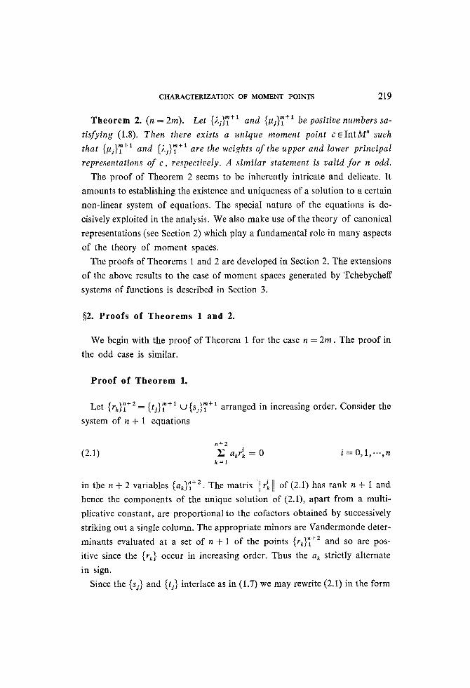
Theorem 2. (n = 2m). Let (2j)'~ +1 and {/~),~+1 be positive numbers sa-

tisfying (1.8). Then there exists a unique moment point c ~ I n t M" such that r ,,n+l m+l (#j~l and {2i} x are the weights of the upper and lower principal

representations of c, respectively. A similar statement is valid for n odd.

The proof of Theorem 2 seems to be inherently intricate and delicate. It

amounts to establishing the existence and uniqueness of a solution to a certain

non-linear system of equations. The special nature of the equations is de-

cisively exploited in the analysis. We also make use of the theory of canonical

representations (see Section 2) which play a fundamental role in many aspects

of the theory of moment spaces.

The proofs of Theorems 1 and 2 are developed in Section 2. The extensions

of the above results to the case of moment spaces generated by Tchebycheff

systems of functions is described in Section 3.

w P r o o f s of T h e o r e m s 1 and 2.

We begin with the proof of Theorem 1 for the case n = 2m. The proof in

the odd case is similar.

P r o o f of T h e o r e m 1.

:t l -m+1 U r ~ m + l L e t {rk}] +2 = ( j J1 lSj)l arranged in increasing order. Consider the

system of n + 1 equations

n+2

(2.1) ~2 akrfk = 0 i = O , 1,- . . ,n k = l

in the n + 2 variables {a~}] +2. The matrix ]] r~ ]] of (2.1) has rank n + 1 and

hence the components of the unique solution of (2.1), apart from a multi-

plicative constant, are proportional to the cofactors obtained by successively

striking out a single column. The appropriate minors are Vandermonde deter-

minants evaluated at a set of n + 1 of the points {rk}] +2 and so are pos-

itive since the {rk} occur in increasing order. Thus the ak strictly alternate

in sign.

Since the {s j} and {ti} interlace as in (1.7) we may rewrite (2.1) in the form


m + l m + l

i = 0 , 1 , . . . , n (2.2) )-2, 2it) = ~ Iris j , j=l j=l

where now 2 j = a z j _ 1 > 0 and / ~ j = - a z j > 0 , j = l , 2 , . . . , m + l . Setting

the components of c equal to the values of (2.2), and fixing the multiplying m + l m + l

constant so that Co = Y~ 2j = ~ /t j = 1, we obtain a moment point j=l j=l

c~ IntM" with the desired principal representations. It is clear that c is actually

in the interior of M" since a boundary point of M" has a unique representation

involving at most p < m + 1 points with index value < n / 2 while the

expression in (2.2) indicates that c has index (n + 1)/2.

The remainder of this section is devoted to the proof of Theorem 2. To

this end it is first essential to introduce additional terminology and review

several other facts concerning moment spaces described more fully in [3].

A representation of an interior point c ~ I n t 11l,+1 is called canonical if

I(c) < n +____.22 For any c ~ Int 11l,+ 1 and any prescribed t* ~ [0,1] there exists = 2 "

a canonical representation of c involving the root t*. The roots of canonical

representations also satisfy certain interlacing properties. Indeed, suppose

that a and a* are the measures associated with two different representations

of c e lnt 11~,+1 and suppose a is canonical. Then for every pair of interior

roots t j , tj+ 1 of a there exists a point of increase of a* in (t~, ti+ 1). This fact

implies, in particular, that no two canonical representations of an interior

point of 111,+ 1 may share an interior root. For the proof of the above as-

sertion we refer to Karlin and Studden [3, Chapter 2].

We are now prepared to establish the main result of the paper.

P r o o f o f T h e o r e m 2.

The proof will be elaborated in a series of lemmas. The first group of

lemmas establish the existence of a moment point with the desired principal

representations. The remaining lemmas provide the demonstration of the

uniqueness assertion.

We proceed by induction. Assuming that the theorem is proved for n = 2m


we wish to show its validity for n = 2m + 1. The inductive step proceeding

from n = 2 m + l to n = 2 m + 2 is carried out in a similar manner while

the initial step corresponding to n = 1 is trivial.

The confirmation of the existence of a moment point in In tM"(n = 2m + 1)

possessing lower and upper principal representations with weights J'2 ~m+ t jj1 and

{#~}~+z is equivalent to establishing the existence of points {tj}~ +1 and

{sj}~ '+2 interlacing in the manner

(2.3) 0 = s t < tl < "'" < sm+t < tm+t < Sin+2 = 1

and satisfying the non-linear system of equations

m + l m+2

(2.4) d t = • 2 j t J - Z /zfl~ l = l , 2 , . . . , n . j = l j = t

m + l

= 21t~ + ~ ( - # f i ~ + a j t ~ ) - / ~ m + 2 = 0 j=2

We will show that a solution of (2.4) possessing property (2.3) exists by emp-

loying a continuity method.

Consider the open simplex A in E"-1 defined by

A : {7 = (~)1,~2, "" ,~2m)] 0 < 71 < ~)2 '<~ "'" < ~)2m < 1} .

It is convenient to also label the components of a point ~ of A in an alternate

manner. Thus we will frequently use the identification

~1 : ( ~ l , 7 2 , ' " , Y 2 m ) = (s2, t 2 , ' " ' S m + l ' t m + l ) " We now define a mapping f of A

into E n-~ with components

m + l

( 2 . 5 ) f t (~)=f l ( s2 , t2,"' ,Sm+l,tm+l) ~ I t -- (--/~fly q- 2jtj) - / lm+2, j=2

l = 1 , 2 , . . . , n - 1 .

The mapping f is locally 1:1 on A. In fact an explicit computation of the

Jacobian of the transformation yields

222 SAMUEL K A R L I N and LARRY SCHUMAKER

(2.6) J ( f l , f 2 , ' " , f . -2 , f . -1 )

\82, t2~ "" ",Sm+ 1, tin+ 1 /

m + l (O,l,..., n-3, n-2) (n-a)! 1-I (-'~j#j)

= j = 2 V \ s 2 ~ t 2 , . . . , Sm+l , tm+ 1

where V denotes the Vandermonde determinant

( 0, 1, . . . , p ~ = det l[ ~J II~.Joo" V \~o, ~ , "", ~ /

Since the 2j and #i are by stipulation strictly positive numbers and the Vander-

monde determinant is well known to be non-zero when evaluated at distinct

points, we see that the Jacobian never vanishes on A and therefore the map-

ping f is locally homeomorphic. Moreover, f (from direct inspection) and

the inverse mapping f - 1 which is well defined locally by virtue of the implicit

function theorem, see Apostol [1, p. 147], possess continuous partial deri-

vatives of all orders. Viewed globally, f - 1 could conceivably be multivalued

although we will later prove t h a t f -1 is actually 1 : 1 in thelarge (i.e., 1:i on

the range f(A)).

Our first lemma shows the existence of a point in A which is mapped into

zero by f .

L e m m a 1. There exists a point ?o in A such that f(?o) = O.

ProoL

If we set t t = 0 in (2.4), examination of the first n - 1 equations in terms of

the variables s2, t2,"',Sm+ 1, tin+ 1 reveals that they are precisely the equations

corresponding to the existence of a moment point in In tM "-1 (n - 1 = 2m)

with the weights of its lower and upper principal representations prescribed as

(2.7)

1, 1 - /~1 ' ' 1 - Pl) (lower)

~2 ~3 ~m+2 / 1 p l ' 1 - px' ' 1 ~ p l j (upper).

C H A R A C T E R I Z A T I O N OF MOMENT POINTS 223

These sets of weights clearly satisfy the restrictions (1.8) for the case n = 2m

and hence invoking the induction hypothesis we obtain a solution of the

first n - 1 equations of (2.4) (with tl = 0) which we designate by {t~ +x and c 0 ~ m + l 0 0 0 0 0 �9 ? = (s2,t2,...,sm+l,t,~+O is in the simplex A since the ~sj 12 The point

roots of the principal representations of a moment point in M n-1 inter-

lock in the manner

(2.8) 0 0 0 < s ~ 1 7 6 < Sm+l<tra+l<l .

An equivalent expression of this fact (cf. (2.4) for t~ = 0 and (2.5)) is that

the point ?o of A is mapped into zero by the func t ionf . The proof of Lem-

ma 1 is complete.

Appealing to the implicit function theorem we deduce the existence of

functions {tj(t)}~ '+l and {sj(t)}7 +1 of class C~(-e,e) such that

(2.9) ~(t) = (s2(t), t2(t ) ,'--,Sm+ l ( t ) , tin+ l(t))

is a point of A and

(2.1o) .fz(s2(t), t2(t), ...,sin+ 1(0, t,,+ 1(0) = - 2it z,

1 = 1 , 2 , . . . , n - 1

for all t 6 ( - e , e ) where e is positive and sufficiently small. Of course,

~(0) = ~o. The relations (2.10) may be written out explicitly as

(2.~1) m + !

at(t) = 21[h(t)] t + ~, (-pj[s2(t)] t + 2j[tj(t)] t) -/2m+2 = 0 j = 2

I = 1 , 2 , - . . , n - 1

where we choose t l ( t )= t. We underscore an important property of the

components of (2.9) in the next lemma.

L e m m a 2. The functions {tj(t)}~ '+1 and (sj(t)}~ +1 appearing in (2.9)

are monotone increasing for t 6 ( - 8 , e ) .


P r o o L

Differentiating (2.11) with respect to t yields

(2.12) 21t~ -~ dtl(t) m+l {_p.sl._ 1 dsj(t) dtj(t)t at + ~ ~ ~ ~ --,t-i-- + ~jtj-~ dt / = 0 . /=2

I=1,2, . . . ,n-1.

The equations (2.12) may be regarded as a system of n - 1 homogeneous

equations in the n unknowns {2flj)~ +1 and " ,~m+l , , ~--lljSj)2 where tj and sj are

shorthands for dtj(t)/dt and dsj(t)/dt respectively. The matrix of the system

has rank n - 1 and hence

(2.13) 2fl~ = xV ( 0'1'2' . . . , n - 3 , n - 2 )

\ t l , s 2 , t 2, ""~Sj, Sj+ I, "'%Sin+l, tm+ l l

j = 1 ,2 , . . . ,m + 1.

,1, . . . , n - 3 , n - 2 ) Pis~

xV\q,s2, "',tj-l,tj,-",sin + 1, tin+ a

j = 2 ,3 , . . . ,m + 1

where ~c is a fixed constant. Since the point ?(t) of (2.9) is contained in A the

determinants occurring in (2.13) are all strictly positive. But by choice t] _--I

and by stipulation 21 > 0 from which we infer that tc > 0, and thus t~. > 0 r

and sj > 0 ( j = 2 ,3 , . . . ,m + 1).

The relations (2.11) are satisfied also when t = e if {tj(e)}~ '+t and

{s/(e))~ '+1 are chosen suitably. In fact, consider a sequence e, increasing to e.

Lemma 2 tells us that the components of (2.9) increase to finite limits; viz.

t j(8,)--, t / 0 (2.14) j = 2,3,. . . ,m + l

sj(~r) --, sA0

or what is the same

(2.15) r(8,) --, r(,)


where ?(e) = (Sz(e), t2(e),..., St, + l(e), tm+ t(e)) and the equations (2.11) hold for

t = e. By continuity we infer, since ?(e,) ~ A for all r , that

s2(0 ) < s2(e ) = < t2(e ) = < ... = < sm+t(e ) = < tm+l(e ) = < 1

i.e., ?(z) is contained in the closure of A which we denote by A. The point

y(e) is either in A or lies on the boundary of A. It is on the boundary of

A only if at least two successive components of ?(e) are equal and/or

if ~,~_l(e) = tm+l(e) = 1. The next lemma shows that the first contingency

is impossible, i.e., if ?(e) as constructed above belongs to BdA then necessarily

0 < e < ?2(8) < 73(~) < "'" < ?,-2(e) < ?,-x(e) = 1.

L e m m a 3. Let ?(t) be defined as above for t e [0,e]. Then

O < t < s 2 ( t ) < t 2 ( t ) < ' " < s , ~ + t ( t ) < t m + l ( t ) < = l for O<_t<=e.

Proof.

For each t E [0, e] the equations (2.11) may be interpreted as asserting that

(tj(t)}'~ +l and m+2 {sj(t)} t , (st(t)-- O,sm+2(t)-- 1) qualify as the roots of two

distinct canonical representations of some moment point c(t)~ In tM ~-1. As

noted above, however, two canonical representations may not share an interior

root and hence the t / s and s /s are distinct. Since the points are in the in-

dicated order for t = 0, invoking the continuity we see that they remain in

this order for all t~ [0,e]. Further, since 0 < s2(0) and S2(t ) is strictly

monotone increasing, t < SE(t ) if e is sufficiently small.

We now extend the definition of ?(t) up to the "upper face" of the bound-

ary o f A (BdA) defined by ?2,, = 1.

L e m m a 4. There exists a point t in (0,1) and a curve ?(t) of the form

(2.9) defined on [0 , [ ] whose components are continuously differentiable

such that the relations (2.11) hold for all 0 <- t <_ t. Furthermore, ?( t )sA

for 0 <_ t < t while ?(~) is in the "upper face" of Bd A, i.e., ?z,,(~) = tm+ t(t) = 1

and 0 < t -- ?t(t) < ? 2 ( l ) • -.. < ? 2 m _ t ( t ) < 72ra(t) = 1 .


Proof.

The required y(t) is determined on [0,~] by the preceding analysis. Lemma

3 tells us that ?(e) is either in the open simplex A or in the "upper face" of

Bd A. In the latter circumstance the proof of the lemma is complete. On the

other hand, if t , ,+l(e)< 1 then 7(e)~A and the implicit function theorem

applies at ~ with initial point ?(e). The theorem affirms the existence of a

unique curve ?(t) possessing components of continuity class C t defined on

an open neighborhood ( e - 6 , ~ + 6) of the point e with 6 > 0, such that

7(t)~A and (2.11) holds. Owing to the local homeomorphic character of f

we infer that ?(t) is of continuity class C 1 on a - 6 < t < e + 6. Lemma 2

continues to apply implying that the components of 7 are monotone increas-

ing. Employing a limiting argument as previously we may construct the point

7(e + 6). Lemma 3 now applies on [e,e + 6] which shows that 7(e + 6) either

belongs to A or to the "upper face" of BdA. This process of extension of

7(0 can be repeated on increasing t intervals. It necessarily ends for some

f < 1, however, since by Lemma 3, t < t,,+~(t) so that for some f in (0,1)

the point 7(0 lies on the "upper face" of BdA.

The existence part of Theorem 2 will be complete if we show that

m + l ra+2

(2.16) d,(t) = • 2j[ti(t)]" -- ~E pi[sj(t)]" j = l j = l

changes sign as t traverses the interval [0, Q since d,(t) is clearly a continuous

function of t. This is the intent of the next lemma.

Lemma 5. Let d.(t) be defined as in (2.16). Then d.(O)<0 and

d.(t) > O.

ProoL

To compute the sign of d,(0) we regard (2.11) and (2.16) for t = 0 as n

linear equations in the n variables whose solutions are the constants (2j]~ n+l

and {-# i}~ +z (recalling that h ( 0 ) = 0). Solving by Cramer's rule for -P2

yields


1, 2, . . . , n - l , n )

-/a2V \sz(O),t2(O),...,tm+ l(O),Sm+2(O)

A, 2, . . . ,n-2 , n - 1 x = d.(0)(- 1)"-~v( | .

t 2 (0), S 3 (0), "", t m + l(0),S m + 2 ( 0 ) 1

The determinants are strictly positive because of (2.8) and hence d,(0)< 0

since /z z > 0 and n is odd.

To compute d,(0 we regard (2.11) and (2.16) for t = t as n equations in

n variables with the solution given by the constants {2i}~', (-ILj}~ +l and

(2m+1--/tin+2) (noting that tin+l(0= Sin+2(?)= 1). Solving for hi yields

/1, 2, . . . , n - l , n )

~l V~q( O,S2( O,'",Sm+ l( O, tm+ l( O

1, 2, . . . , n -2 , n - 1 1

= dn(O(- 1)"-1 V \S2(O, t2(O,...,Sm+t(O, tm+l(~)]

where as before the determinants being Vandermondian are strictly positive

while 21 > 0 and n is odd implying that d,(?) > 0.

Our next task is to establish the uniqueness part of Theorem 2. The first

lemma proves that the point 7(0 =(Sz(t),t2(t),'",Sm+l(t),tm+i(t)) in A such

that (2.11) holds is uniquely determined.

Lemma 6. Suppose O< t 1 < 1 and let 7(tl) and ~(ti) be two points

of A such that (2.11) is satisfied. Then y(t l )= ~(ti).

P r o o L

The proof is by reductio ad absurdum. Suppose that V(tl) is distinct from

~7(ti). Applying the implicit function theorem at the point tl with the two

different initial points y(ti) and ~(tl) and repeating the process as carried out

in Lemmas 2 and 4 we obtain two distinct curves v(t) and ~7(t) in A defined on

[0,tl] whose components are all monotone increasing. Now if y(0)= ~(0)

we violate the fact that the mapping f from A into E "-I defined in (2.5)

is locally 1:1 since ~(0 and ~(t) describe distinct curves.


On the other hand, if yr(0) # 7r(0) for some r, 1 < r < n, we have produced

two distinct solutions (namely ?(0) and ~(0)) to the problem in the moment

space Int M"-1 with prescribed weights (2.7). This is incompatible with the

uniqueness assertion of the inductive hypothesis. Thus in either circumstance

we have a contradiction thereby implying the result of the lemma.

We need the following additional lemma.

L e m m a 7. Let 7(t) be a curve o f the form (2.9) in A such that (2.11)

holds. Then the function dn(t) defined in (2.16) is strictly increasing, i.e.,

d',(t) > O.

P r o o L

Consider the system of equations (2.12) coupled with the equation

m+ 1 d'(t) n- 1 , n- I , , - 1 , = n21t 1 t x + n 2jtj t j). ( - - f l j S j Sj JF

j = 2

Solving for 21t~ = 21 by Cramer's rule yields

( D"-~d'(+" ~ , 1 , ' " , n - 3 , n - 2 ) 21V (O, 1 , . . . , n - 2 , n - 1 ] _ , - , , ,OV

\ t l , S 2 , . . . , S m + l , t m + l / n s 2 , t 2 , . . . , S m + l , t m + i "

By Lemma 2 the points appearing in the Vandermonde determinants are

distinct and arranged in increasing order and consequently the determinants

are strictly positive. Since 21 > 0 by specification and n is odd we deduce

that d',(t) > O.

We are prepared to complete the proof of the uniqueness assertion of

Theorem 2.

St )+m+ 1, S t )m+l L e m m a 8. Let ~ j j t {sj}~ '+t and ~,./jl , {~j}~,+l be two sets o f

roots satisfying (2.3) and (2.4). Then t~= tj, j = 1 , 2 , . . . , m + 1 and

s = ~j, j = 2 , . . . ,m + 1.


ProoL

Assume that the sets of roots are not identical. Invoking the implicit func-

tion theorem as above we start at t~ and Tt (say i~ > t~) and generate two

curves ~(t) and ~(t) in A such that (2.11)is satisfied for all t e [ 0 , ? l ] .

By Lemma 6 these curves coincide for all t~ [0, rl] . Since by hypothesis (2.4)

is satisfied we have d,(tl)= d, (? l )= 0, contradicting the fact that dn(t) is

strictly monotone increasing (Lemma 7). This contradiction proves the lemma.

w Extens ions .

The results of Section 2 have been specifically elaborated in the context

of the system of functions {1, t,...,t"} which generate the classical reduced

moment space 111,+1. In this section we indicate the extensions of these re-

sults to the case of generalized moment spaces induced by a Complete Tche-

bycheff system of functions {ui}~. For the relevance, utility and importance

of general Tchebycheff systems in analysis and applications, we refer the

reader to [3].

Let uo(t),ul(t),...,u,(t) be continuous functions on [a,b]. The set

{ui}~ is said to be a Tchebycheff(T) system provided the determinants

t~ ) (3.1) U = det[] u,(tj) n > 0

\ O,l,...,n

for all a < to < tt < ".. < t, ~ b. The set {ui}~o is called a Complete Tche- bycheff (CT) system if {ui} k is a T-system for k = 0,1,.-., n. I f ui ~ C"[a, b], i = 0,1,. . . , n then {ui}~ is referred to as an Extended Tchebycheff(ET) system

provided

(3.2) u* ) = detl[ u,(ti)[I > 0 \ 0, 1, . . . ,n ./

whenever a < t 0 < t l < . . . _ < t . < b where if for some j and p

t i _ l < t j = t j + 1 . . . . . t j+p<t j+ j ,+ l , then the j + l + l st row of (3.2) is (t) (0 (t) to be replaced by the vector of components [Uo(tj),ut (tj),...,u, (tj)]


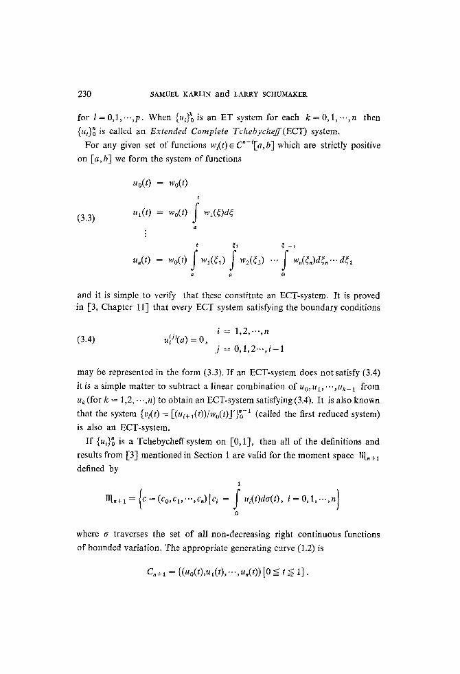
for l = 0 , 1 , . . . , p . When {ui}ko is an ET system for each k = 0 , 1 , . . . , n then

{ui}g is called an Extended Complete Tchebycheff(ECT) system.

For any given set of functions w~(t)~ c"-i[a,b] which are strictly positive

on [a, b] we form the system of functions

(3.3)

uo(t ) = Wo(t )

u~(t) = Wo(t)

t

f w~(~)d~ a

Un(t) = Wo(t) f wl('t) ~ W 2 ( ' 2 ) " ' " f Wn(,n)d,n...d,1 a a 0

and it is simple to verify that these constitute an ECT-system. It is proved in I-3, Chapter 11] that every ECT system satisfying the boundary conditions

i = 1,2, . . . ,n (3.4) u~J~(a) = 0,

j = 0 , 1 , 2 . . . , i - 1

may be represented in the form (3.3). I f an ECT-system does not satisfy (3.4)

it is a simple matter to subtract a Iinear combination of Uo,Ul,...,Uk_t from

uk (for k = 1,2,...,n) to obtain an ECT-system satisfying (3.4). It is also known

that the system {Vi(t ) = [-(Ui+ l(t))/Wo(t)]'}"o-1 (called the first reduced system)

is also an ECT-system.

If {ui} ~ is a Tchebycheff system on [0,1], then all of the definitions and

results from [3] mentioned in Section 1 are valid for the moment space lq,+l

defined by

1

,0 o / 0

where a traverses the set of all non-decreasing right continuous functions

of bounded variation. The appropriate generating curve (1.2) is

C,+ t = ((Uo(t),ut(t), ...,u,(t)) [0 -< t ~< 1}.


When {ui}~ is an ECT-system with u o - 1 the arguments of Theorem 2

proceed mutatis mutandis. The determinants occurring in the proof are po-

sitive owing to the ECr-property. The analog of the Jacobian (2.6) is positive

since as noted above the first reduced system {[(ui+t(t))/Wo(O]'}"o -1 is also

an ECT-system.

Theorem 2 is also valid if {ui}~ is merely a CT-system on [0,1] with uo --- 1.

This is proved by using a standard perturbation technique. Specifically, (see

[3]), we form the modified system of functions

1

�9 ~ ~/2-~ ~ u , ( x ) d x , i = O, 1 , . " , n

For e > 0, {ui(e;t)}~ is an ECT-system when {tt,}~ is a CT-system. Then for

each e > 0 (let n = 2m + 1, say) there exists a unique moment point c(e) s Int M"

and roots {ti(e)}7 '+1 and {s/~)}'~ +z satisfying (2.3) such that

m+l m+2 (3.5) c/(e) = ]~ ).flt~(t/~)) = ~2 i~jui(sj(~)) , i = 0 , 1 , . . . , n

j = l j = l

are the lower and upper principal representations of c(~). Now executing a

standard diagonal selection procedure corresponding to a sequence of ek

decreasing to zero, we produce {rj}~ '+1 and {~i}~ "+2 such that t j ( e k ) ~ 7i,

j = 1,2, . . . ,m + 1 and Sj(ek)'-->gj, j = 1 ,2 , . . . ,m + 2. Then clearly {?j}7 +~

and {gj}~+2 are the roots of the lower and upper principal representations

of a moment point ~.

REFERENCES

1. Tom M. Apostol, Mathematical Analysis, Addison-Wesley, Reading, Mass., 1960. 2. S. Karlin and L. S. Shapley, "Geometry of Moment Spaces," Mem. Am. Math. Soc.

No. 12, 1953. 3. S. Karlin and W. Studden, Tchebycheff Systems with Applications in Analysis

and Statistics, Interscience, New York, 1966. 4. M. G. Krein, "The Ideas ofP. L. Cebysev and A. A. Markov in the Theory of Limiting

Values of Integrals and Their Further Developments," Am. Math. Soc. Transl., Ser. 2,12,3-120. 5. G. Szeg6, Orthogonal Polynomials, revised edition, New York, 1959.

DEPARTMENT OF MATHEMATICS, STANFORD UNIVERSITY,

STANFORD, CALIFORNIA, U.S.A. (Received March 25, 1966)

characterization of moment points in terms of christoffel numbers

Documents