characterization of the germania spraberry unit …
TRANSCRIPT

CHARACTERIZATION OF THE GERMANIA SPRABERRY UNIT FROM
ANALOG STUDIES AND CASED-HOLE NEUTRON LOG DATA
A Thesis
by
BABAJIDE ADELEKAN OLUMIDE
Submitted to the Office of Graduate Studies of Texas A&M University
in partial fulfillment of the requirements for the degree of
MASTER OF SCIENCE
August 2004
Major Subject: Petroleum Engineering

CHARACTERIZATION OF THE GERMANIA SPRABERRY UNIT FROM
ANALOG STUDIES AND CASED-HOLE NEUTRON LOG DATA
A Thesis
by
BABAJIDE ADELEKAN OLUMIDE
Submitted to Texas A&M University in partial fulfillment of the requirements
for the degree of
MASTER OF SCIENCE
Approved as to style and content by:
______________________________ ______________________________ David S. Schechter Jerry L. Jensen (Chair of Committee) (Member)
______________________________ ______________________________ Robert R. Berg Stephen A. Holditch (Member) (Head of Department)
August 2004
Major Subject: Petroleum Engineering

iii
ABSTRACT
Characterization of the Spraberry Unit from Analog Studies and Cased-Hole Neutron
Log Data.
(August 2004)
Babajide Adelekan Olumide, B.Sc., University of Ibadan, Ibadan
Chair of Advisory Committee: Dr. David S. Schechter
The need for characterization of the Germania unit has emerged as a first step in the
review, understanding and enhancement of the production practices applicable within the
unit and the trend area in general.
Petrophysical characterization of the Germania Spraberry units requires a unique
approach for a number of reasons – limited core data, lack of modern log data and
absence of directed studies within the unit.
In the absence of the afore mentioned resources, an approach that will rely heavily on
previous petrophysical work carried out in the neighboring ET O’Daniel unit (6.2 miles
away), and normalization of the old log data prior to conventional interpretation
techniques will be used.
A log-based rock model has been able to guide successfully the prediction of pay and
non-pay intervals within the ET O’Daniel unit, and will be useful if found applicable
within the Germania unit. A novel multiple regression technique utilizing non-parametric
transformations to achieve better correlations in predicting a dependent variable
(permeability) from multiple independent variables (rock type, shale volume and
porosity) will also be investigated in this study.
A log data base includes digitized formats of gamma ray, cased hole neutron, limited
resistivity and neutron/density/sonic porosity logs over a considerable wide area.

iv
DEDICATION
I dedicate this work to God Almighty, who has shown me mercy and showered upon me
abundant blessings that have made it possible to be who I am and where I am today, and
guide who I will become tomorrow.
To my father and mother for being loving, caring and supportive parents, and a formative
influence in my life. To my brothers and sisters who shared my joys and bore my pains
and still loved me after it all.
To my wife and 9 month old daughter, Isi and Oluwateniola, for being my support and
joy ever since they came into my life.
To my cousin Jide and his wife Tola, for their good will, support and encouragement
through the challenges I faced during this period.
Finally, to my late brother, Adebowale, who I wish could be here to share all my joys.

v
ACKNOWLEDGMENTS
My sincere gratitude goes to my advisory committee chair, Dr. D.S. Schechter, who has
been patient and supportive all through my indecision to the completion of this thesis. I
am thankful for his open demeanor and being a subtle taskmaster. Also, I thank Dr.
Jensen for his constructive criticism and input towards improving the quality of this
work.
Thanks also to Dr. Erwinsyah Putra for his invaluable support to the Naturally Fractured
Group as a whole, as well as his role as a mentor and resource base for me during the
course of my program at A&M.
The US Department of Energy (DOE) and Pioneer Natural Resources (PNR) for funding
and providing useful data towards the successful completion of this project.
To Dr. Tom Blasingame for his encouragement and making things possible for me during
my period at Texas A&M.
To the friends from all backgrounds that I have made while I have been at A&M.

vi
TABLE OF CONTENTS
Page
ABSTRACT....................................................................................................................... iii
DEDICATION................................................................................................................... iv
ACKNOWLEDGMENTS .................................................................................................. v
LIST OF TABLES........................................................................................................... viii
LIST OF FIGURES ........................................................................................................... ix
CHAPTER I INTRODUCTION...................................................................................... 1
Project overview ..................................................................................................... 1 Area of interest........................................................................................................ 2 Rock-log model....................................................................................................... 4 Lithofacies based model ......................................................................................... 6 Non-depositional model.......................................................................................... 6 Permeability estimation techniques ........................................................................ 9
Explicit probabilistic techniques................................................................. 9 Implicit probabilistic techniques............................................................... 10
Porosity estimation................................................................................................ 11 Gamma ray................................................................................................ 11 Clay content .............................................................................................. 12
Log normalization................................................................................................. 13 Histogram.................................................................................................. 16 Crossplots.................................................................................................. 16 Overlays .................................................................................................... 16
CHAPTER II DATA REVIEW (E.T. O’DANIEL) ...................................................... 17
Core sampling ....................................................................................................... 17 Depth matched core-log playback ........................................................................ 18 Lithology............................................................................................................... 22
CHAPTER III DATA ANALYSIS ............................................................................... 25
Log conversions and normalization ...................................................................... 25 Gamma ray................................................................................................ 25
Gamma ray maps .......................................................................... 25 Gamma ray normalization............................................................. 28
Neutron logs.............................................................................................. 31 Standardization of neutron log units ............................................. 31 Conversion from neutron units to linear porosity units ................ 32
Porosity ................................................................................................................. 33 Corrections for porosity ............................................................................ 34
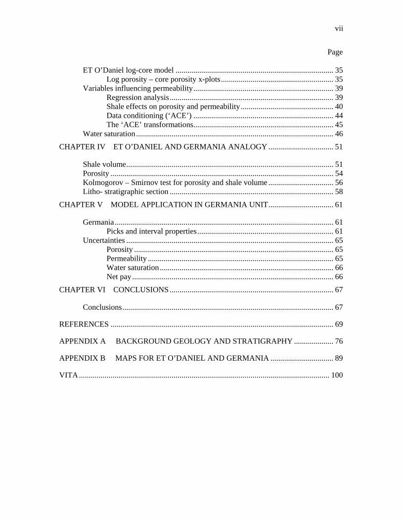
vii
Page
ET O’Daniel log-core model ................................................................................ 35 Log porosity – core porosity x-plots......................................................... 35
Variables influencing permeability....................................................................... 39 Regression analysis................................................................................... 39 Shale effects on porosity and permeability............................................... 40 Data conditioning (‘ACE’) ....................................................................... 44 The ‘ACE’ transformations....................................................................... 45
Water saturation .................................................................................................... 46
CHAPTER IV ET O’DANIEL AND GERMANIA ANALOGY ................................. 51
Shale volume......................................................................................................... 51 Porosity ................................................................................................................. 54 Kolmogorov – Smirnov test for porosity and shale volume ................................. 56 Litho- stratigraphic section ................................................................................... 58
CHAPTER V MODEL APPLICATION IN GERMANIA UNIT................................. 61
Germania............................................................................................................... 61 Picks and interval properties..................................................................... 61
Uncertainties ......................................................................................................... 65 Porosity ..................................................................................................... 65 Permeability .............................................................................................. 65 Water saturation ........................................................................................ 66 Net pay ...................................................................................................... 66
CHAPTER VI CONCLUSIONS ................................................................................... 67
Conclusions........................................................................................................... 67
REFERENCES ................................................................................................................. 69
APPENDIX A BACKGROUND GEOLOGY AND STRATIGRAPHY .................... 76
APPENDIX B MAPS FOR ET O’DANIEL AND GERMANIA ................................ 89
VITA............................................................................................................................... 100
viii
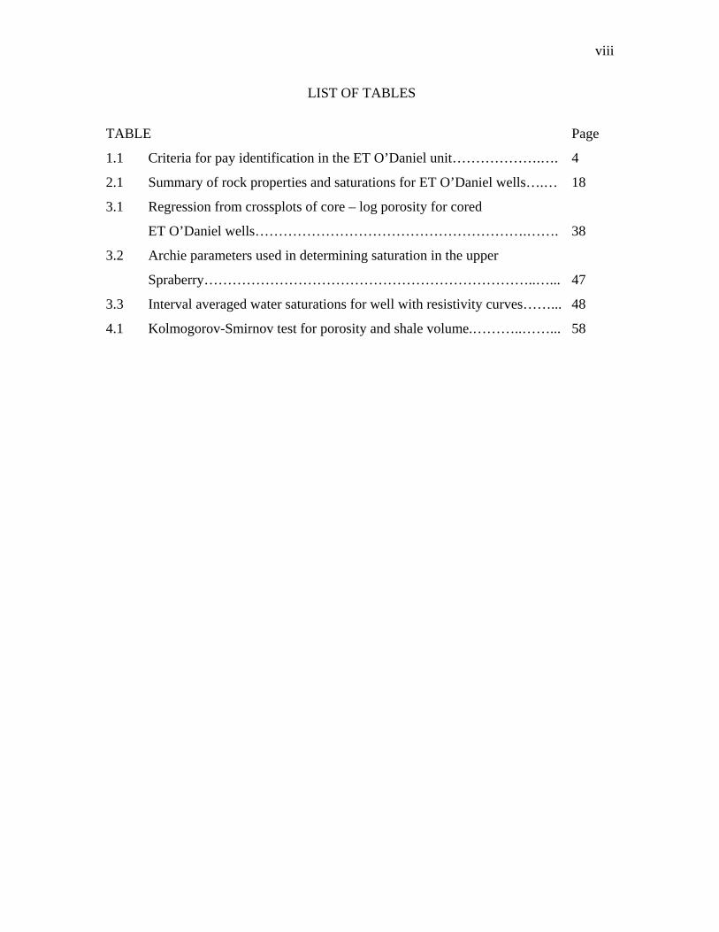
LIST OF TABLES
TABLE Page
1.1 Criteria for pay identification in the ET O’Daniel unit……………….…. 4
2.1 Summary of rock properties and saturations for ET O’Daniel wells….… 18
3.1 Regression from crossplots of core – log porosity for cored
ET O’Daniel wells………………………………………………….……. 38
3.2 Archie parameters used in determining saturation in the upper
Spraberry……………………………………………………………..…... 47
3.3 Interval averaged water saturations for well with resistivity curves……... 48
4.1 Kolmogorov-Smirnov test for porosity and shale volume.………..……... 58

ix
LIST OF FIGURES
FIGURE Page
1.1 Unit locations within the Spraberry trend area…...……………………….. 3
1.2 Crossplot of shale volume and porosity for well ET 47, 1U sand………... 5
1.3 Porosity - permeability crossplot for the primary rock types identified...... 7
1.4 Identification of pay based on shale volume and effective porosity
cutoffs………………………..…………………………………………... 8
1.5 Non-linearity of the different models for estimating clay content
using gamma ray…………..……………………………………………… 13
1.6 The log analysis process………………………………………….……… 14
2.1 Map of cored well locations in the ET O’Daniel pilot area….………….. 17
2.2 Typical core - log playback in the 1U interval…………………………... 19
2.3 Crossplot of shale volume and porosity for well ET 37, 1U sand……….. 20
2.4 Typical core – log playback in the 5U interval..…………………………. 21
2.5 Crossplot of shale volume and porosity for well ET 37, 5U sand……….. 22
2.6a Crossplot for lithology identification in 1U sand for well ET 37..….…… 23
2.6b Crossplot for lithology identification in 5U sand for well ET 37...……… 23
3.1 Minimum gamma ray values for ET O’Daniel unit in the 1U
sand interval………………………………………………………….…... 26
3.2 Maximum gamma ray values for ET O’Daniel unit in the 1U
sand interval…………………………………………………………..….. 27
3.3 Variations in response from the gamma ray curves in ET O’Daniel…….. 28
3.4 Histogram and CDF for wells 36, before and after normalizing
against well 26……………………………………………………………. 29
3.5 Corrected gamma ray distribution for ET O’Daniel wells.………………. 30
3.6 Normalized gamma ray values in 1U and 5U regions of upper
Spraberry, ET O’Daniel unit...………………………………………..….. 31
3.7 Effects on quality of porosity data from density and neutron
porosity tools…………………………………………………………….. 34
3.8 Crossplot of core porosity and log porosity for ET 39, 1U sand………… 36

x
FIGURE Page
3.9 Crossplot of core porosity and log porosity for ET 39, 5U sand………… 37
3.10 Playback of log and core porosity for ET 39, 1U sand………………….. 38
3.11 Playback of log and core porosity for ET 39, 5U sand………………….. 38
3.12a ET 39 crossplot for shale volume and permeability……………………... 40
3.12b ET 47 crossplot for shale volume and permeability……………………... 40
3.13a ET 39 crossplot for log porosity and permeability……………………..... 41
3.13b ET 47 crossplot for log porosity and permeability……………………..... 42
3.14a ET 39 crossplot for shale corrected porosity and permeability………….. 43
3.14b ET 47 crossplot for shale corrected porosity and permeability………….. 43
3.15 Playback of results from conventional regression and ACE regression.... 46
3.16 Saturation profile matched for ET 38, 1U using Rw 0.035 ohm-m
and m 1.7………………………………………………………………… 49
3.17 Saturation profile matched for ET 40, 1U using Rw 0.035 ohm-m
and m 1.7………………………………………………………………… 50
4.1 Statistics of Vsh values for ET O’Daniel, 1U sand..……………………. 51
4.2 Statistics of Vsh values for ET O’Daniel, 5U sand..……………………. 52
4.3 Statistics of Vsh values for Germania, 1U sand..……………………….. 52
4.4 Statistics of Vsh values for Germania, 5U sand..……………………….. 53
4.5 IQR and mean values of shale volume and porosity for ET O’Daniel
and Germania units..……………………………………………….……. 53
4.6 Statistics of porosity values for ET O’Daniel, 1U sand..……………….. 54
4.7 Statistics of porosity values for ET O’Daniel, 5U sand..……………….. 55
4.8 Statistics of porosity values for Germania, 1U sand…………………….. 55
4.9 Statistics of porosity values for Germania, 5U sand…………………….. 56
4.10 Kolmogorov - Smirnov test on porosity function, 1U sand..……………. 57
4.11 Gross thickness map of the 1U sand..…………………………………… 59
4.12 Lithostratigraphic section A-A’ with datum at top of 1U interval………. 60
5.1 Payzone prediction based on rock model for GSU 146A, 1U sand...…… 61
5.2 Estimate of rock types in GSU146A, 1U sand from shale volume –
porosity crossplot..………………………………………………………. 62
xi
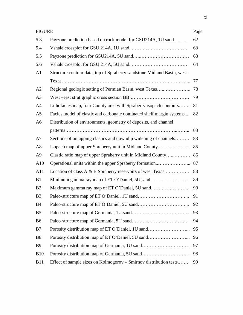
FIGURE Page
5.3 Payzone prediction based on rock model for GSU214A, 1U sand….…… 62
5.4 Vshale crossplot for GSU 214A, 1U sand..……………………………… 63
5.5 Payzone prediction for GSU214A, 5U sand.…..………………………… 63
5.6 Vshale crossplot for GSU 214A, 5U sand..……………………………… 64
A1 Structure contour data, top of Spraberry sandstone Midland Basin, west
Texas……………………………………………….……………………... 77
A2 Regional geologic setting of Permian Basin, west Texas…..…………….. 78
A3 West –east stratigraphic cross section BB’.……………………………… 79
A4 Lithofacies map, four County area with Spraberry isopach contours……. 81
A5 Facies model of clastic and carbonate dominated shelf margin systems.... 82
A6 Distribution of environments, geometry of deposits, and channel
patterns……………………………………………………………..…….. 83
A7 Sections of onlapping clastics and downdip widening of channels……… 83
A8 Isopach map of upper Spraberry unit in Midland County…..……………. 85
A9 Clastic ratio map of upper Spraberry unit in Midland County…...………. 86
A10 Operational units within the upper Spraberry formation..………………... 87
A11 Location of class A & B Spraberry reservoirs of west Texas.…………… 88
B1 Minimum gamma ray map of ET O’Daniel, 5U sand.…………………... 89
B2 Maximum gamma ray map of ET O’Daniel, 5U sand.………………….. 90
B3 Paleo-structure map of ET O’Daniel, 1U sand…………………………... 91
B4 Paleo-structure map of ET O’Daniel, 5U sand…………………………... 92
B5 Paleo-structure map of Germania, 1U sand……………………………… 93
B6 Paleo-structure map of Germania, 5U sand……………………………… 94
B7 Porosity distribution map of ET O’Daniel, 1U sand……………………... 95
B8 Porosity distribution map of ET O’Daniel, 5U sand……………………... 96
B9 Porosity distribution map of Germania, 1U sand………………………… 97
B10 Porosity distribution map of Germania, 5U sand………………………… 98
B11 Effect of sample sizes on Kolmogorov – Smirnov distribution tests.…… 99
1
CHAPTER I
INTRODUCTION
Project overview
The Spraberry trend area is a unitized hydrocarbon production Basin in the heart of west
Texas. The major production comes from fine grained, low permeability siltstones and
sandstones, enhanced by an intricate network of natural fractures. Carbonate and
siliclastic (submarine fans) depositional episodes during the Permian era make up the
lithofacies of the Spraberry unit.
Up to date production from the Basin is estimated at about 800 million barrels of oil and
3 trillion cubic ft of gas from over 8000 active wells1, this figure could range between 8 –
12% of the projected OHIP.
Of particular interest is the ET O’Daniel and Germania Spraberry units, two of eleven
units operated by Pioneer Natural Resources. Extensive reservoir characterization work
has been carried out in the ET O’Daniel based on recent core and log data acquisition,
production data and simulation studies. The Germania Spraberry unit on the other hand
lacks core and modern log data, and has not been characterized beyond pulse and tracer
tests to analyze fracture trends and performance.
A preliminary step in the implementation of an enhanced recovery process within the unit
is the characterization of the reservoir (petrophysics and fracture properties and fracture
network).
This study is concerned with the log based characterization of the Germania unit and will
focus on the petrophysical evaluation of the upper Spraberry unit, particularly the
productive 1U and 5U intervals.
__________________
This thesis follows the style of SPE Reservoir Evaluation & Engineering.

2
A database of 85 log suites, primarily consisting of gamma ray and old cased hole
neutron logs are available for this study. Core based relationships developed in the ET
O’Daniel unit are borrowed upon to aid the characterization of this field, and will
generally suffice due to the similar depositional environment and proximity of the units
from one another (6.2 miles).
Established criteria for predicting rock type and pay zones in the ET O’Daniel will be
applied if found applicable to Germania and will guide subsequent characterization
efforts in the unit.
Area of interest
The Spraberry trend area spreads over an area of approximately half-a-million acres and
is trapped by complex updip pinchouts and facies changes within the thick upper
Spraberry producing interval. A few fields are simple anticlinal structures like Benedum
and Pegasus. The regional fracture patterns are enhanced by anti-clinal folds producing a
locally commercial reservoir at Pegasus2,3 (see Fig. A11 in appendix A).
The E.T. O’Daniel unit and the Germania unit are adjacent units at the north end of the
Spraberry trend area. These fields are 2 of 11 fields operated by the Pioneer Natural
Resources (PNR) and are located in the Midland County area of west Texas.

3
Fig. 1.1 – Unit locations within the Spraberry trend area.
The distance between the two fields is estimated to be about 6.2 miles based on inter-well
distance measured from boundary wells (see Fig 1.1).
Whereas the ET O’Daniel has been the subject of major studies regarding fracture
patterns4-6, log - core analysis7-11 and waterflood and CO2 injection pilot projects1,12-14, no
major investigation of the lithofacies or fracture characteristics of the Germania unit has
been performed. Fracture trends on a gross scale by way of pulse and tracer tests is the
basis of predicting flow behavior within the Germania unit.
Due to the proximity of the ET O’Daniel unit to the Germania unit as well as the
depositional environment within the four County area15, 16 (Midland, Glasscock, Upton
and Reagan) it becomes logical to superimpose the conclusions drawn from the
petrophysical evaluation of the ET O’Daniel unit upon the Germania unit.
Bearing this in mind, further discussions on the characterization work regarding this area
will be focused on the ET O’Daniel unit.
Glasscock Co
Reagan CoUpton Co
Midland Co
Martin Co Howard Co
Glasscock Co
Reagan CoUpton Co
Midland Co
Martin Co Howard Co
Pioneer Natural Resources’ Pioneer Natural Resources’ Spraberry Unit PositionSpraberry Unit Position
Spraberry Trend AreaSpraberry Trend Area
Pioneer Natural Resources’ Pioneer Natural Resources’ Spraberry Unit PositionSpraberry Unit Position
Spraberry Trend AreaSpraberry Trend Area
E.T. O’Daniel Co-op
Atlantic PilotPreston Unit
Humble & Heckman Pilots
Driver UnitMcDonald Pilot
Germania Unit
6.25miles

4
Rock-log model
Gamma ray and old cased hole neutron logs form the bulk of the electric logging data
available within the ET O’Daniel. More recently, array induction, density and neutron
porosity data have been acquired in pilot areas within the unit. This acquisition is
localized and hence the older neutron logs are an indispensable source for wide scale
characterization of the field.
A log based rock model10,11 was developed for the trend area using shale content
(gamma ray) and porosity as discriminatory criteria for rock type. In this model,
classification is made for 3 rock types – A, B and C.
Table 1.1 summarizes the identifiers for the rock model within the upper Spraberry
operational units based on effective porosity and shale content17.
Table 1.1 - Criteria for pay identification in the ET O’Daniel unit.
Formation Rock Type Shale Volume PHIE Facies Fluorescence Pay UnitA > 7% SS Strong yes 1U, 5U
Upper Spraberry B < 7% DS+SS Weak 2U, 3U, 4UC > 15% SH+DS+SS None muddy zones
SS - SiltstoneSH - ShaleDS - Dolomite
< 15%no
More recently, ‘Thin section’ analysis of core samples within the upper Spraberry were
point count analyzed to establish framework, cement mineralogy and diagenetic features
of the rock8. Especially useful in identifying and classifying samples was x-ray
diffraction (XRD) and scanning electron microscope (SEM) analysis to determine clay
mineralogy and proportions of clay minerals within the various rock types. Prior to the
results of the study, a direct relationship was assumed between porosity and gamma ray
response and permeability and gamma ray response, which for the most part is true. What
Schechter and Banik9 also showed was that clay content is a significant factor in

5
predicting overall permeability. Sands with low clay content have a high overall
permeability within the 1U.
Rock type A is the only reservoir quality rock identified within the upper Spraberry,
types B and C are non-reservoir quality rock. A crossplot of the shale volume and the
effective porosity provides an easy method of rock identification (Fig. 1.2).
Rock Type A – Massive, clean siltstone, low clay and dolomite content. Strongly
fluorescent with low water saturation.
Rock Type B – Low clay, low dolomitic content with weak or no fluorescence and high
water saturation.
Rock Type C – Muddy clay rich zones that do not fluoresce.
Fig. 1.2 – Crossplot of shale volume and porosity for well ET 47, 1U sand.

6
Lithofacies based model
Eight separate lithofacies18 are defined based on sedimentological, compositional and
textural features of core samples. These are broadly divided into those with reservoir
potential, and non-reservoir potential deposits.
Potential reservoir deposits consist of:
Type 1 – Massive siltstones and very fine grained sandstones
Type 2 – Thin bedded siltstones and very fine grained sandstones exhibiting basal
intervals of massive sandstone grading vertically into parallel or cross laminated
sandstone and siltstone.
Type 3 – Thin bedded, graded, cross laminated siltstones and very fine grained
sandstones, interbedded with dark grey shales
Non-reservoir lithofacies consist of:
Type 1 – Massive silty dolostone and dolomite-cemented siltstone
Type 2 – Black shales containing phosphatic nodules and abundant pyrite
Type 3 – Thin bedded argillaceous siltstone showing abundant soft sediment deformation
Type 4 – Bioturbated argillaceous siltstone in which scattered silt-size grains of quartz
and feldspar float in a groundmass of detrital clays
Type 5 – Parallel and finely laminated siltstone and silty shale.
Non-depositional model
A more generic classification of the rock types of the upper Spraberry that relate better
with rock quality based on non-depositional factors is developed using petrographic
analysis, petrophysical analysis and compositional information18.
To avoid confusion, the log based rock model will be referred to as the secondary
classification, and the generic model as primary.

7
The core based primary model shows that the upper Spraberry can be divided into six
distinct rock types:
Type 1 – Coarse siltstones and very fine grained sandstones (A)
Type 2 – Laminated or patchy siltstones and very fine grained sandstones (B)
Type 3 – Silty dolomite mudstones (C)
Type 4 – Very patchy dolomitic siltstones (D)
Type 5 – Shale and silty shale(E)
Type 6 – Highly laminated siltstones (F)
Type 1 is the only rock type with reservoir potential.
Fig. 1.3 – Porosity - permeability crossplot for the primary rock types identified18.
The rock log model has proved consistent in the preliminary identification of pay and
non-pay reservoirs. Deflections from gamma ray corresponding to lower values were
used to define probable reservoir quality sandstones in the past, with typical cutoffs
ranging from 45 – 50 API units. With these cutoffs, individual zones within the 1U, 2U,
3U, 4U and 5U intervals were thought to be possible pay zones in the ET O’Daniel wells.
Core data has however shown that only the 1U and 5U exhibit any fluorescence,
moreover, the intermediate intervals 2U to 4U, despite showing gamma ray values in the
8
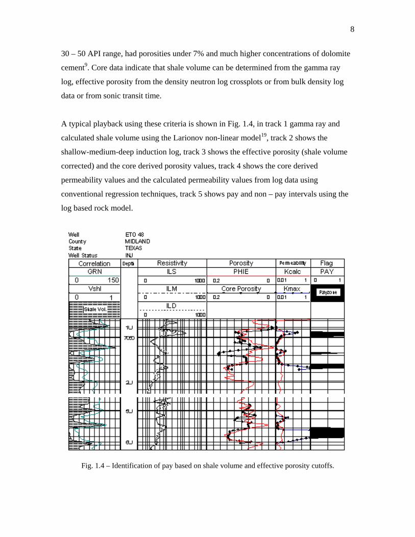
30 – 50 API range, had porosities under 7% and much higher concentrations of dolomite
cement9. Core data indicate that shale volume can be determined from the gamma ray
log, effective porosity from the density neutron log crossplots or from bulk density log
data or from sonic transit time.
A typical playback using these criteria is shown in Fig. 1.4, in track 1 gamma ray and
calculated shale volume using the Larionov non-linear model19, track 2 shows the
shallow-medium-deep induction log, track 3 shows the effective porosity (shale volume
corrected) and the core derived porosity values, track 4 shows the core derived
permeability values and the calculated permeability values from log data using
conventional regression techniques, track 5 shows pay and non – pay intervals using the
log based rock model.
Fig. 1.4 – Identification of pay based on shale volume and effective porosity cutoffs.

9
Permeability estimation techniques
An important parameter which is key to the rock model is the estimation of permeability
from log data. Conventional methods estimate k from e-logs and consist of building
models between regularly spaced core plug measurements and logs, without paying much
attention to the various scales of core plug sampling20.
In uncored intervals k are usually estimated from well test, production or log data. Early
attempts used porosity (unsatisfactorily), which is not unexpected as the permeability is
related to pore throat size rather than pore volume. More recently, a host of relationships
have been investigated between permeability and other rock attributes. Permeability as a
function of porosity and irreducible water saturation21, or bulk density, neutron porosity,
interval transit time and gamma ray22. A multi-dimensional histogram approach, deriving
permeability based on bulk density, interval transit time and gamma ray was investigated
successfully by Schlumberger. Some other functional relationships investigated are
related to formation resistivity, normalized spontaneous potential and borehole Stoneley
waves22,23, 24, 25.
In analyzing permeability dependency on single or multiple variable, regression as well
as discriminant analysis are the most widely used techniques of evaluation.
These techniques can be classified into two broad groups: Explicit probabilistic methods
and implicit irobabilistic methods.
Explicit probabilistic techniques
Regression Analysis – This is a crossplot of 2 dimensions, used to predict values in
intervals without core data and wells without core data. This method assumes the
functional form of the relationship between the prediction and response variable is
unknown. The drawbacks of this method is that it over-simplifies reality and tends to
smooth out real variations or trends in the data, because more often than not, other
independent factors influence the prediction, therefore making a two dimensional

10
prediction inadequate for reliability. Sub-dividing the data into logically coherent groups
in geologically correlated zones often improves the overall correlation.
Multiple Regression analysis includes additional variables or non-linear regression
techniques.
The ‘ACE” algorithm originally proposed by Friedman and Breiman26 provides a method
for estimating optimal transformations for multiple regression that result in a maximum
correlation between a dependent (response) random variable and multiple independent
(predictor) random variables. Xue et. al.27, went further to develop a non-parametric
approach that optimizes based on no predetermined functional form, derived solely based
on the data set.
Discriminant analysis – This is a multi variate technique designed to separate samples
into groups based on relationships found in a training set of data. The relationship must
be such that they can be defined explicitly and must be linear combinations of functions
of the predictor variables.
Implicit probabilistic techniques
Probabilistic or database methods are intrinsic (or implicit) relationships of data compiled
in a multi dimensional database. A value of y is read from a database corresponding to a
value of x. In this way the implicit relationship between the data are preserved.
N-Dimensional histogram – When the x corresponding to y concept is expanded to
include additional variables, the approach becomes an ‘n-dimensional histogram’, and the
discrimination of the dependent variable is generally improved. This method has the
following advantages over regression techniques in that it has the ability to preserve the
subtle relationships between variables, it fully utilizes the shape characteristics of the data
and it has the ability to incorporate soft data such as facies type into the database to
define the categories of qualitative histograms.
11
Cluster analysis – This is a multi-variate technique for classification of samples into
groups based on little or no prior knowledge of that grouping. Simple cluster analysis
does not use the information on facies known from the cored interval, but instead
attempts to find natural groupings, called clusters based on the estimator variable.
Porosity estimation
Porosity is determined from 3 basic log types that measure porosity directly (neutron) or
indirectly (density and sonic). Where a neutron count based porosity value is known from
the older neutron logs, a conversion algorithm28, may be used to convert counts per
second or any CPS derived unit (environmental units, API cps, etc) which exhibits a
logarithmic scale of porosity to porosity values on a linear scale.
Where the density, neutron porosity and photoelectric effect curves are available,
porosity measurements based on shale corrected lithology model can be reliable and
consistent over a wide range of rock types29. No matrix parameters are required for this
model unless light hydrocarbons are present. Shale corrected density and neutron data are
used as input in this model and results depend on shale volume calculations and density
and neutron shale properties selected for the model. Therefore porosity should be
compared to core data and corrected accordingly till a suitable match is obtained between
both data sets.
Where limited suite of porosity logs are available, a model based on the shale corrected
density, shale corrected neutron or shale corrected sonic is used29.
Gamma ray
The Gamma Ray log is a continuous recording of the intensity of the natural gamma
radiations emanating from the formations penetrated by the borehole vs. depth.

12
In sedimentary formations, since the radioactivity can be attributed mainly to the clay
minerals, the gamma ray log can be used to distinguish between shale and non-shale
formations and to estimate the clay content of shaly formations.
Clay content
Clay or shale content can be quantified using a shale index from values given by the
gamma ray log. Different models are available for quantifying this index:
General linear form
cleanshl
cleanrawshl GRGR
GRXV
−−
= (1.1)
Other models used to modify the index to account for various degrees of non-linearity
between the gamma ray response and the clay content are available:
Larionov’s model for tertiary rocks
)12(083.0 7.3mod_ −= shlV
ifiedshlV (1.2)
Larionovs’ model for older rocks
)12(33.0 0.2mod_ −= shlV
ifiedshlV (1.3)
Stiebers’ model
shl
shlifiedshl V
VV23mod_ −
= (1.4)
Claviers’ model 5.02
mod_ ))7.0(38.3(7.1 +−−= shlifiedshl VV (1.5)

13
0
0.25
0.5
0.75
1
0 0.25 0.5 0.75 1
Shale index
Shal
e vo
lum
e LinearLarionov (old)ClavierStieberLarionov (ter.)
Fig. 1.5 - Non-linearity of the different models for estimating clay content using
gamma ray.
Log normalization
Well log normalization is a fundamental part of well log analysis, and is one of the
necessary steps for arriving at accurate rock quality descriptors. The foundation of the
integrated log analysis process is the core, well test and log database30. The short comings
in the foundations of the analysis ultimately influence the quality of the final estimations
of permeability, the interdependence of the descriptors are shown in Fig. 1.6.
Errors in the database will trickle up to affect shaliness, porosity and water saturation
calculations. Also errors in shaliness calculation will cause additional errors in porosity
and water saturation because these calculations also depend on shaliness. When
everything is done correctly useful values of permeability and effective permeability can
be obtained from integrated studies.

14
In excess of fifty percent of all well logs are erroneous, Neinast and Knox31 base this
percentage on an analysis of 1986 suites of well logs containing more than 34 million
curve feet. The basic sources of error are tool malfunction, incorrect tool design,
inconsistent shop and field calibration, and operator error. All but ten percent of the
incorrect logs may be corrected and the data used quantitatively.
Fig. 1.6 – The log analysis process30.
Hunt30 in his analysis, suggests that about 65 - 70% of gamma rays logs, 50% of density
logs, 40% - 50% of neutron logs and 5% - 10% of sonic logs require some normalization
to correct for variances in field calibrations of logging tools. After normalization well log
data can be effectively integrated, correlated and calibrated with core data. The resulting
correlations can be extended vertically to include layers that were not cored, and laterally
Environm
ent
Other studies
Garbage out
History
Norm
alization
Calibration
Swφ
keffective
Core, welltest & Log data
k
ShalinessE
nvironment
Other studies
Garbage out
History
Norm
alization
Calibration
Swφ
keffective
Core, welltest & Log data
k
Shaliness

15
to wells across the study area. The difference in scale of measurement of the two data sets
must be taken into account. Core data have a scale of cubic inches, while log data have a
scale of cubic meters and well test data have a scale of acre-feet.
The normalization procedure to correct log data requires the following31:
- Digitize the well log data
- Select corresponding lithologic intervals
- Accumulate and present data in appropriate form (Histograms, etc)
- Compute porosity and water saturation
- Compare with core analysis
- Map to reveal anomalies
Digitization – The individual curves are depth matched either prior to data capture in
ASCII format or if post processing software is available to correct depth anomalies. All
heading data is combined with the log values to allow pertinent corrections to be made in
subsequent calculations.
Interval selection – Correlation of stratigraphic intervals is of extreme importance. The
earth changes radically in a vertical direction and gradually in a lateral direction.
Appropriate corresponding lithological sections must be chosen so that comparison of
similar intervals may be accomplished. Every effort should be made to eliminate pay
zones or other zones of interest as data for correlation prior to normalization.
Data presentation – Data must be accumulated in a form that allows rapid and concise
corrections. Variations in thickness of explicit sections is eliminated by presenting the
information in statistical format. The basic concept is the formation of patterns that the
analyst recognizes and compares to make the proper corrections. Three methods of data
presentation are histograms, crossplots and overlay.

16
Histogram
The histogram is made by plotting the percent frequency of occurrence of data on the
abscissa against the log unit value on the ordinate. The mean and standard deviation are
calculated along with the mode, maximum and minimum values, and the net and gross
number of samples used in the histogram. Histograms of discriminated or complete log
values may be prepared for specific correlated intervals. The individual frequency
histograms may be compared with similar histograms from other wells, with core derived
histograms, or with mass histograms or entire regions or fields.
Crossplots
Crossplot techniques for lithology and porosity determination have been in use for
several years. Additional advantage of dual porosity device data may be taken if the
lithology is known or assumed. Errors in individual tools may be detected when the
crossplotted data falls outside the range delineated by constant mineral lines. When three
porosity logs are available, the data can be used to develop an M-N plot and allow
corrections to properly compute porosity. The procedure is to first histogram and
normalize individual logs, then verify and refine the normalization with crossplots.
Overlays
This is a simple process of correlating and overlaying similar type logs and noting the
difference.
Computation and comparison – After the data has been normalized, the water saturation,
porosity, lithology, permeability, etc. are computed on a foot by foot basis and compared
to the weighted average core data to determine the degree of compatibility
Mapping – Contour maps are generated on selected intervals. Generally porosity and
water saturation are the parameters used to confirm normalization. All drastic changes
and abrupt highs and lows are rigorously verified as to validity.
17
CHAPTER II
DATA REVIEW (E.T. O’DANIEL)
Core sampling
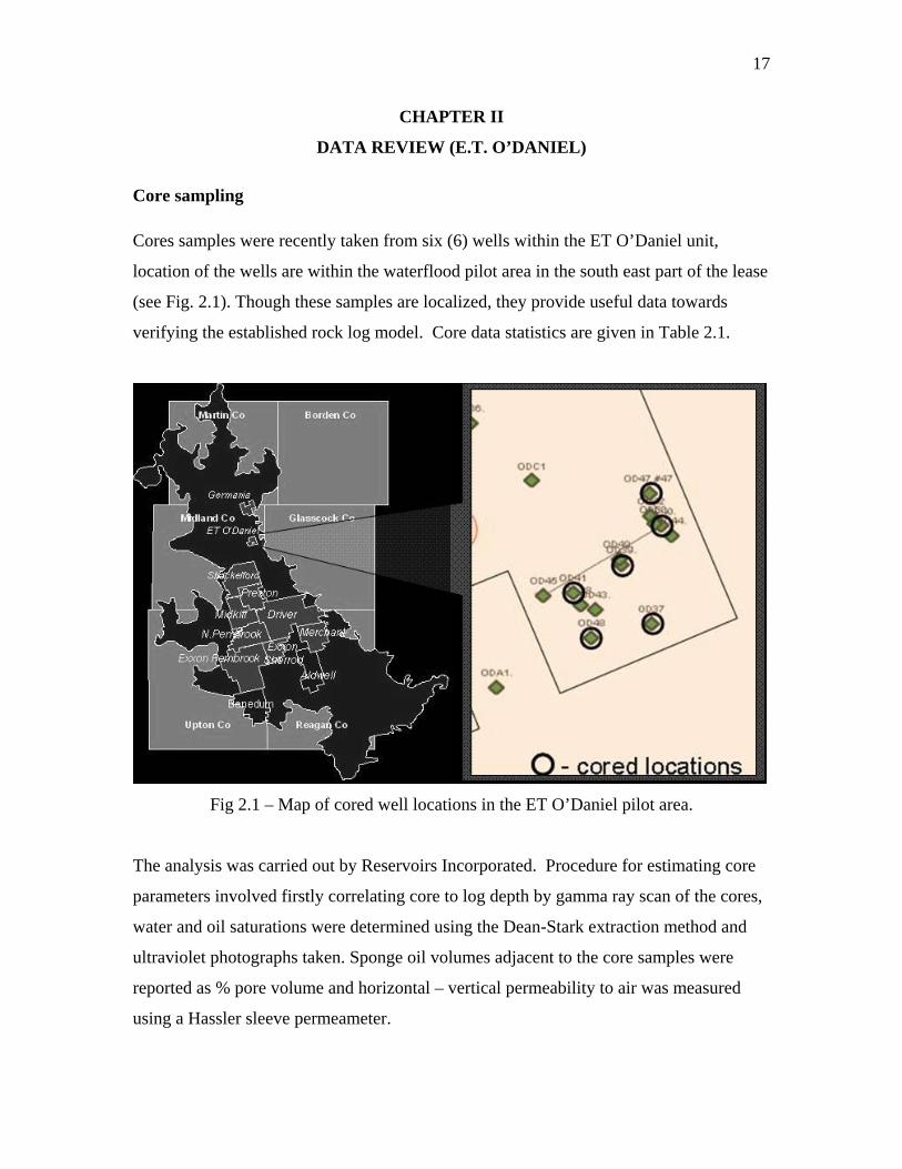
Cores samples were recently taken from six (6) wells within the ET O’Daniel unit,
location of the wells are within the waterflood pilot area in the south east part of the lease
(see Fig. 2.1). Though these samples are localized, they provide useful data towards
verifying the established rock log model. Core data statistics are given in Table 2.1.
Fig 2.1 – Map of cored well locations in the ET O’Daniel pilot area.
The analysis was carried out by Reservoirs Incorporated. Procedure for estimating core
parameters involved firstly correlating core to log depth by gamma ray scan of the cores,
water and oil saturations were determined using the Dean-Stark extraction method and
ultraviolet photographs taken. Sponge oil volumes adjacent to the core samples were
reported as % pore volume and horizontal – vertical permeability to air was measured
using a Hassler sleeve permeameter.
18
The core values obtained are integrated into the log database using the Geographix
software, and depth matched using the log and core porosity response as a guide. This
ensures that all data sampled from the logs with reference to the core data are for the
same interval.
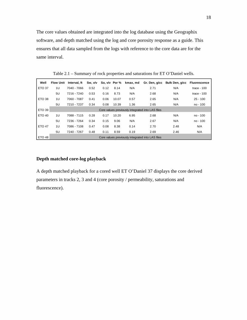
Table 2.1 – Summary of rock properties and saturations for ET O’Daniel wells.
Well Flow Unit Interval, ft Sw, v/v So, v/v Por % kmax, md Gr. Den, g/cc Bulk Den, g/cc Fluorescence
ETO 37 1U 7040 - 7066 0.52 0.12 8.14 N/A 2.71 N/A trace - 100
5U 7216 - 7240 0.53 0.16 8.73 N/A 2.68 N/A trace - 100
ETO 38 1U 7060 - 7087 0.41 0.06 10.07 0.57 2.65 N/A 25 - 100
5U 7210 - 7237 0.34 0.08 10.39 1.36 2.65 N/A no - 100
ETO 39
ETO 40 1U 7088 - 7115 0.28 0.17 10.20 6.95 2.68 N/A no - 100
5U 7236 - 7264 0.34 0.15 9.06 N/A 2.67 N/A no - 100
ETO 47 1U 7086 - 7108 0.47 0.08 8.38 0.14 2.70 2.48 N/A
5U 7240 - 7267 0.48 0.11 8.59 0.19 2.69 2.46 N/A
ETO 48
Core values previously integrated into LAS files
Core values previously integrated into LAS files
Depth matched core-log playback
A depth matched playback for a cored well ET O’Daniel 37 displays the core derived
parameters in tracks 2, 3 and 4 (core porosity / permeability, saturations and
fluorescence).
19
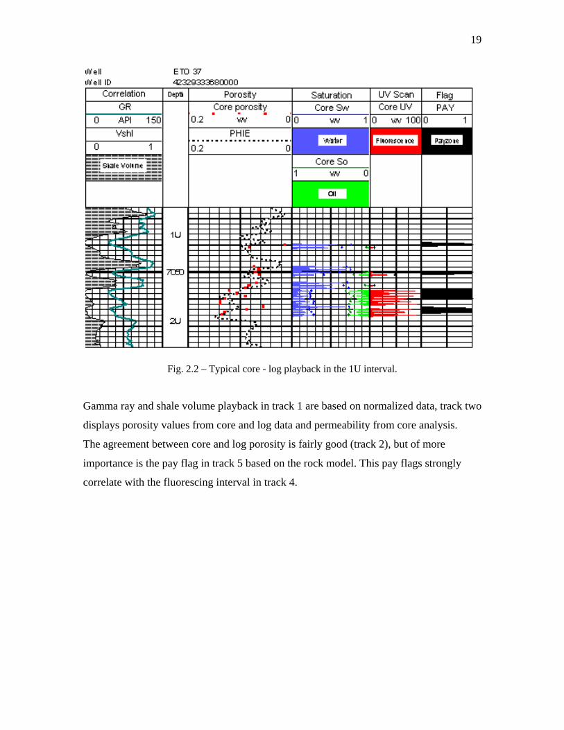
Fig. 2.2 – Typical core - log playback in the 1U interval.
Gamma ray and shale volume playback in track 1 are based on normalized data, track two
displays porosity values from core and log data and permeability from core analysis.
The agreement between core and log porosity is fairly good (track 2), but of more
importance is the pay flag in track 5 based on the rock model. This pay flags strongly
correlate with the fluorescing interval in track 4.

20
Fig. 2.3 – Crossplot of shale volume and porosity for ET 37, 1U sand.
The shale volume - porosity crossplot gives a quantitative indication of the rock types
within the analyzed interval. In Fig. 2.3 the amount of rock type B is minimal, while type
A and C are evenly distributed in the 1U interval for well ETO37.

21
Fig. 2.4 – Typical core - log playback in the 5U interval.
The payflag and fluorescing interval for this unit (5U) correlate well after a depth shift
based on core porosity and log porosity matching. The playback resulting from this
optimal correlation is shown in Fig. 2.4.

22
Fig. 2.5 – Crossplot of shale volume and porosity for well ET 37, 5U sand.
A number of observations are evident from figs. 2.2 to 2.5, these are that the low shale
intervals of the 1U and 5U units are almost exclusively payzones or type A rocks, while
the higher shale intervals are exclusively non-hydrocarbon bearing sands. Also a estimate
of the productive intervals (net pay) account for about 50% of the gross sand in the 1U
unit and about 40% of the gross sand in the 5U intervals. Other well analyzed also
displayed similar trends as observed in wells ETO 37.
The 1U and 5U pay zones are easily identified by integrating whole core analysis and
open hole logs into a calibrated shaly-sand model. The 2U, 3U and 4U zones are not
consistent with this model5, this is due to the large concentration of dolomitic cements,
thus rendering low gamma ray (low shale content) sands in this region as non-pay.
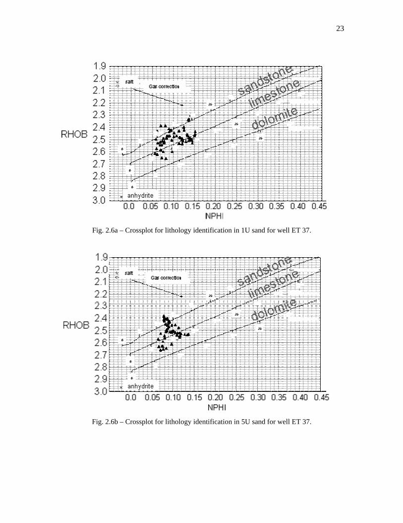
Lithology
The density-neutron crossplots among other uses are invaluable as indicators for
lithology and rock types. Figs. 2.6a – b, show the results of crossplots of neutron density
in the wells in which they are available.
23
Fig. 2.6a – Crossplot for lithology identification in 1U sand for well ET 37.
Fig. 2.6b – Crossplot for lithology identification in 5U sand for well ET 37.

24
The gas correction if applied will tend to shift the data down and right i.e. reduce density porosity
and increase neutron porosity. Shale correction will depend on the type of shale (structural,
laminated or dispersed).

25
CHAPTER III
DATA ANALYSIS
Log conversions and normalization
26 logs are available within the ET O’Daniel unit, including log data for the cored wells.
The wells are a variety of observation wells, injectors and producers.
59 well logs are available within the Germania Spraberry unit. Most of the logs are
neutron logs taken as far back as 1950, with a few recent porosity and resistivity logs.
Log normalizations are performed on both log data sets prior to any transformations or
inferences as to the significance of the log analysis. Illustrative procedures are shown for
ET O’Daniel in the proceeding sections.
Gamma ray
This log forms the basis of pay identification within the Spraberry rock model. It is
therefore important that the gamma ray is scaled appropriately to enable a consistent
shale volume calculation from well to well.
Gamma ray curves for all the logs within the ET O’Daniel database were analyzed, and it
was discovered that no two logs gave the same values at any chosen marker. Though this
is expected, the wide variance in the response across these markers indicate the necessity
for normalization of the gamma ray logs. More so, due to the fact that for a multi-well
analysis, the Shale volume calculations will need to be revised for every well log if this
process is not carried out.
Gamma ray maps
Often mapping techniques are used to discern trends of gamma ray values. These gamma
ray values may sometimes show systematic variation that may often be mistaken as tool
26
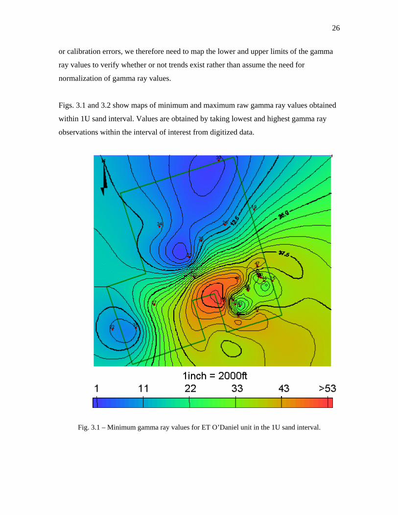
or calibration errors, we therefore need to map the lower and upper limits of the gamma
ray values to verify whether or not trends exist rather than assume the need for
normalization of gamma ray values.
Figs. 3.1 and 3.2 show maps of minimum and maximum raw gamma ray values obtained
within 1U sand interval. Values are obtained by taking lowest and highest gamma ray
observations within the interval of interest from digitized data.
Fig. 3.1 – Minimum gamma ray values for ET O’Daniel unit in the 1U sand interval.

27
Often a bulls eye pattern on a contour map will give away the fact that the data points are
random or lack any systematic variation in space. From the figure above we see that the
NW section of the area is consistently low and the SW is consistently high, this might
indicate a systematic trend. From the maximum gamma ray values in the 1U interval
(Fig. 3.2) we do not see this trend, instead we see bullseye patterns, this will suggest that
the trend in the 1U lacks consistency and hence indicate that normalization is required.
Fig. 3.2 – Maximum gamma ray values for ET O’Daniel unit in the 1U sand interval.
28
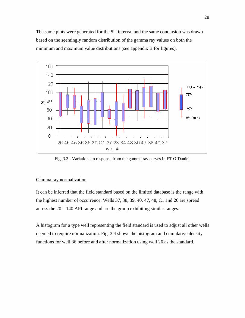
The same plots were generated for the 5U interval and the same conclusion was drawn
based on the seemingly random distribution of the gamma ray values on both the
minimum and maximum value distributions (see appendix B for figures).
Fig. 3.3 - Variations in response from the gamma ray curves in ET O’Daniel.
Gamma ray normalization
It can be inferred that the field standard based on the limited database is the range with
the highest number of occurrence. Wells 37, 38, 39, 40, 47, 48, C1 and 26 are spread
across the 20 – 140 API range and are the group exhibiting similar ranges.
A histogram for a type well representing the field standard is used to adjust all other wells
deemed to require normalization. Fig. 3.4 shows the histogram and cumulative density
functions for well 36 before and after normalization using well 26 as the standard.

29
Fig. 3.4 - Histogram and CDF for wells 36, before and after normalizing against well 26.
A single equation for applying linear adjustments to log data is given by Shier28.
)())((
lowhigh
lowrawlowhighlownorm WW
WXRRRX
−
−−+= (3.1)
A different method used to adjust well log data involves the adjustment of each data point
by a constant value such that the mean of the sample data equals the mean of the type log
data. Thereafter, an ‘Affine’ correction is then applied to the sample data such that the
variance of the sample equals the variance of the type log data. A computer program may
be used to solve for the appropriate shift and correction factor required to match the mean
and variance of the type log data.
Affine Correction32.
µµ +−= )(. rawnorm XfsX (3.2)

30
Xnorm - Normalized well value
Xraw - Actual well value
Rlow - Regional low normalization value
Rhigh - Regional high normalization value
Wlow - Wells lithological low value
Whigh - Wells lithological high value
s.f - Correction factor
µ - Population mean
Fig. 3.5 – Corrected gamma ray distribution for ETO’Daniel wells.

31
Fig. 3.6 – Normalized gamma ray values in 1U and 5U regions of upper Spraberry, ET O’Daniel
unit.
Neutron logs
Standardization of neutron log units
The most common measure of porosity within the GSU log database is counts per second
(cps) and is a measure of the amount of neutrons detected after bombarding the formation
with energetic neutrons at the rate of several millions per second.
The neutron density decreases almost logarithmically with hydrogen richness, which is
why porosity is a logarithmic function of neutron deflections.
The API RP33 recommends a system of neutron unit of calibration in the standardization-
well-logging pit of the University of Houston.

32
One API neutron unit is defined as 1/1000 of the difference between instrument zero (tool
response to zero radiation) and log deflection opposite a 6ft zone of Indiana limestone of
19% porosity.
Conversion from neutron units to linear porosity units
A useful equation for converting a linear scale with respect to counts per second
(logarithmic with respect to porosity), to a linear scale with respect to porosity is given by
Shier28. This method is also known as the two – point method.
)( __10 cpslowcpshigh WWy
normX −= (3.3)
where ))(log())(log()log(log __ φφφφ highcpslowlowcpshighlowhighraw RWRWRRXy −+−=
Xnorm - Normalized well value (porosity, v/v)
Xraw - Actual well value (cps, API, EU)
Rhighφ - Value for high porosity location from core or reliable
log data (known for a particular region, unit – v/v).
Rlowφ - Known value for low porosity location from core or reliable
log data (known for a particular region, unit – v/v).
Whigh_cps - Well value at Rhighφ location (cps, API, EU)
Wlow_cps - Well value at Rlowφ location (cps, API, EU)
(Note: R in this case is not resistivity, but is used to denote regional value of parameter)
This equation is valid for all neutron curves measuring neutron counts irrespective of
units.
The normalization equation requires the input of two lithologies from both a “type” well
and the well being normalized. One lithology input is from a log interval that produces a

33
high log reading and the other is from an interval that produces a low log reading. These
lithology intervals that bound the normalization process are known as normalization
zones. Normalization zones should have a well log response that is consistent from well
to well (as is the case of lithology intervals consisting purely of salt and anhydrite). If
such zones are unavailable, the analyst chooses zones whose behavioral changes are
understood from location to location. This implies that for any one field, many
normalization zones may have to be selected in order to properly limit the high and low
readings of the different curve types being adjusted.
After identifying lithology intervals that will be used for normalization, the characteristic
values of Rlow and Rhigh in these zones must be determined. This is accomplished by
picking a “type” well (or wells) containing normalization zones considered by the
analysts to have the correct well log response. This “type” well (or wells) is then defined
as the standard to which all other curves will be adjusted.
Porosity
Various logs are available that give a direct indication of porosity or matrix density. The
database has mostly cased neutron logs that require conversion from API, cps or EU units
to porosity units (Eq. 3.3). A few other wells have neutron porosity (NPHI, TNPH, TPHI)
or density or acoustic (DT), the later two do not directly measure porosity.
When matrix lithology is known, shale free, and filled with water, all three porosity logs
give the same values of porosity. These conditions are rarely encountered and therefore
adjustments must be made for each of the different logs based on characteristic response
in hydrocarbons and water.
The density log overestimates porosity in hydrocarbons, neutron logs underestimate
porosity in hydrocarbons, and the acoustic log overestimates porosity in hydrocarbons30.
To balance these anomalies out, an average porosity is often taken of the density and

34
neutron logs, in the absence of the density log either the neutron or sonic is used to
estimate porosity.
PHIA = (DPHI + NPHI) / 2 (3.4)
Corrections for porosity
Porosity as earlier mentioned in chapter I, can be obtained from a combination of the
different porosity logs. The preferred log suite will be the density porosity and the
neutron porosity or sonic porosity, unfortunately few wells have the desired combination
and porosity is often resolved from a one dimensional analysis of the available log
(mostly neutron porosity). The playbacks used for analysis are chosen based on
availability of porosity curves for the particular well.
Fig. 3.7 – Effects on quality of porosity data from the density and neutron porosity tools.

35
Shale corrections are highly dependent on mode of shale features within the formation33.
Shalines affects the porosity log response in proportion to the amount, type and
distribution of shale. This distribution may be structural laminated or dispersed shale.
In the 1U and 5U sand units the shale distribution is in the form of laminae. Fig. 3.7
shows the effects of shaliness and gas on porosity values obtained from neutron and
porosity logs.
Effective Porosity – The Effective porosity is less than the total or log measured porosity.
This is due to the residual porosity within the unconnected pore spaces particularly within
the clay minerals. Effective porosity (PHIE) can often be estimated by correcting for the
presence of shale, given by:
PHIE = PHIA (1-Vshl) (3.5)
ET O’Daniel log-core model
Log porosity – core porosity x-plots
The core and log porosity crossplots indicate the level of agreement between core data
and log data. If there is sufficient agreement between both porosities or a relationship
between both data sets can be consistently established, further analysis can be confidently
carried out on the basis of log porosity.

36
Fig. 3.8 - Crossplot core porosity vs. log porosity for ETO’Daniel 39, 1U sand. Light to dark
markers represent a 3rd dimension of increasing shale content on a scale of 0 to 1.
A depth match is performed prior to a crossplot of both porosity values (core and log).
The depth match may be improved by analyzing the degree of correlation obtained for
crossplots based on depth shifting the core data. This is done if a ‘clear’ relationship
cannot be established just by visual analysis.
From regression analysis a best fit equation for the x-plot in 1U was found to be:
Y = 0.050342+0.539983X and R2 = 0.677
And for 5U:
Y = 0.05810 + 0.560472X and R2 = 0.620651

37
Fig. 3.9 - Crossplot core porosity and log porosity for ET 39, 5U sand.
The ET O’Daniel 39 well gave the most consistent core to log relationship of all the
cored wells analyzed, more so within the 1U interval. Table 3.1 shows the summary of
regression results obtained from the crossplots of cored wells in the ET O’Daniel field.

38
Table 3.1 – Regression from crossplots of core – log porosity for cored ET O’Daniel wells.
(Best results are obtained in ETO#39 well).
Core – log porosity discrepancies are observed from the log playbacks and regression
correlations, this is often due to bound water contained in the clays. This is also referred
Well Least Sq. Regression R2 Least Sq. Regression R2
37 y = -0.018494 + 1.12948x 0.542 y = -0.024442 + 0.949273x 0.106
38 y = -0.024815 + 1.049007x 0.230
39 y = 0.050342 + 0.539983x 0.677 y = 0.050810 + 0.560472x 0.621
40 y = 0.050857 + 0.520833x 0.509 y = 0.028280 + 0.662358x 0.396
47 y = 0.017356 + 0.560368x 0.073 y = -0.021898 + 1.243577x 0.073
48 y = 0.014259 + 1.042477x 0.519 y = 0.034999 + 0.748994x 0.776
y = core porosity, x = log porosity
5U1U
39
to as residual porosity earlier mentioned, this results in porosity estimates from logs
exceeding that determined from cores.
Variables influencing permeability
Regression analysis
Various variables often influence the flow capacity of the rock, such as clay mineral
content (shale), distribution, pore throat size / capillary pressure, connate water
saturation, porosity etc. Crossplots of these variables and permeability will often reveal
underlying relationships, furthermore, regression analysis may produce a functional
mathematical model to represent this relationship.
Readily available are porosity and shale volume data obtained from the neutron, density
or acoustic logs and gamma ray logs respectively. Porosity values (PHIE) are verified
against core porosity data (Figs. 3.10 and 3.11).
Figure 3.12 a – b show the shale volume - permeability relationship for wells 39 and 47.
The trend is consistent for all the wells investigated i.e. permeability decreasing with
increasing shale content.

40
ETO 39 Vsh-permeability x-plot
y = 0.3685e-3.2875x
R2 = 0.2196
0.01
0.1
1
10
0 0.2 0.4 0.6 0.8 1
Vshl., v/v
kmax
, md
best fit
Fig. 3.12a - ET 39 crossplot for shale volume and permeability.
ETO 47 Vsh-permeability x-plot
y = 0.7865e-3.7612x
R2 = 0.2862
0.01
0.1
1
10
0.0 0.2 0.4 0.6 0.8 1.0
Vshl, v/v
kmax
, md
best fit
Fig. 3.12b - ET 47 crossplot for shale volume and permeability.
Shale effects on porosity and permeability
Figs. 3.12a and b show the relationship between shale volume and core permeability
values. Within the shaly Spraberry sands, shale is in the form of laminae and therefore we
41
expect a significant effect on the density and neutron porosity log values. Gas effects are
negligible in the Spraberry payzones due to the absence of a gas cap, therefore any
corrections to be made are for shaliness.
Shale corrections are applied to the neutron porosity data as given in Eq. 3.5.
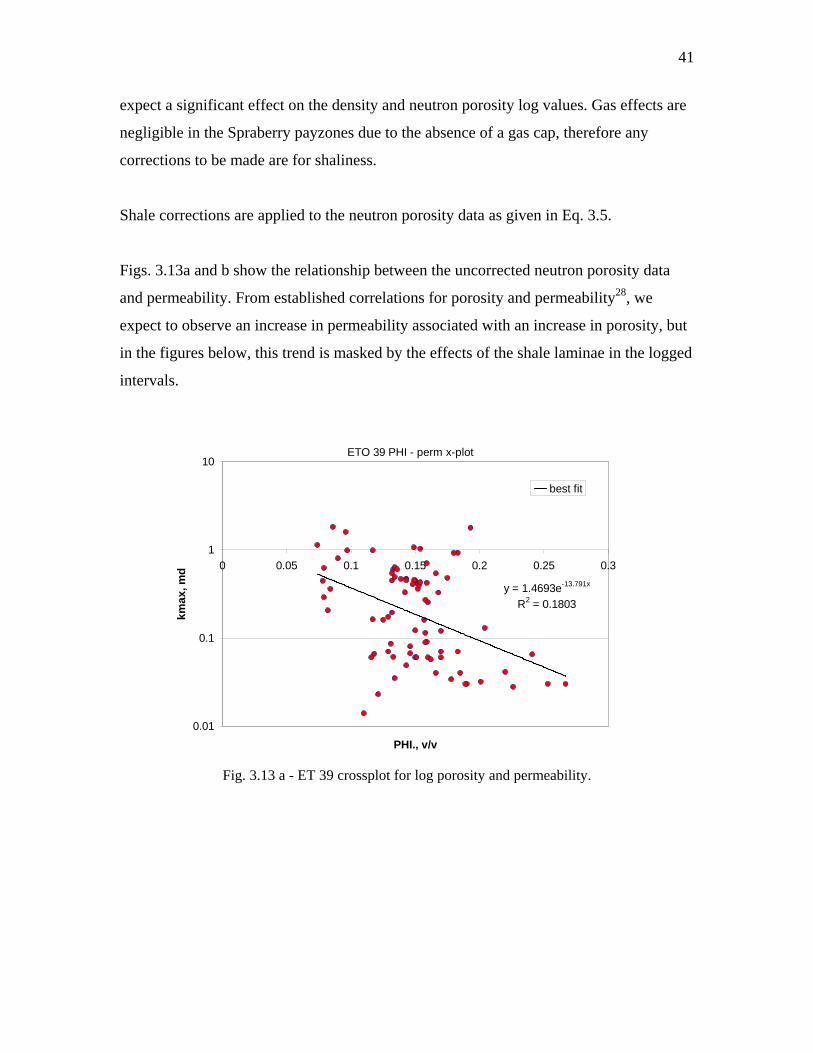
Figs. 3.13a and b show the relationship between the uncorrected neutron porosity data
and permeability. From established correlations for porosity and permeability28, we
expect to observe an increase in permeability associated with an increase in porosity, but
in the figures below, this trend is masked by the effects of the shale laminae in the logged
intervals.
ETO 39 PHI - perm x-plot
y = 1.4693e-13.791x
R2 = 0.1803
0.01
0.1
1
10
0 0.05 0.1 0.15 0.2 0.25 0.3
PHI., v/v
kmax
, md
best fit
Fig. 3.13 a - ET 39 crossplot for log porosity and permeability.

42
ETO 47 PHI - perm x-plot
y = 0.0487e11.089x
R2 = 0.0325
0.01
0.1
1
10
0.0 0.1 0.1 0.2 0.2 0.3
PHI, v/v
kmax
, md
best fit
Fig. 3.13 b - ET 47 crossplot for log porosity and permeability.
From Figs. 3.12, we can see that the shale volume clearly influences the permeability,
therefore we must apply corrections to the log porosity to obtain a useable model for
predicting permeability.
After correcting for shaliness, plots generated for porosity-permeability (Figs. 3.14a and
b) show the functional relationships for predicting permeability based on porosity.
The porosity values from the neutron log are used for this prediction exercise as this is
the available porosity log type within the database, with the exception of only a few wells
which may have both or the three porosity types.

43
ETO 39 PHIe - perm x-plot
y = 0.1334e2.9769x
R2 = 0.005
0.01
0.1
1
10
0 0.05 0.1 0.15 0.2 0.25
PHIe., v/v
kmax
, md
best fit
Fig. 3.14a – ET 39 crossplot for shale corrected porosity and permeability.
ETO 47 PHIe - perm x-plot
y = 0.0069e35.883x
R2 = 0.5153
0.01
0.1
1
10
0.0 0.0 0.0 0.1 0.1 0.1 0.1 0.1
PHIe, v/v
kmax
, md
best fit
Fig. 3.14b - ET 47 crossplot for shale corrected porosity and permeability.
Figures above show the crossplots of 2 of the control wells used to establish a porosity -
permeability relationship. The porosity is corrected for shale (PHIE), and this corrected
porosity is regressed against corresponding core permeability values for each of the wells

44
analyzed. Well ETO 47 gives the best correlation, the resulting relationship between
porosity and permeability is given as:
Y = 0.0069e35.883X and R2 = 0.515
where y = permeability and x = effective porosity for a given well in the zones of
investigation (1U and 5U in this case).
Data conditioning (‘ACE’)
Besides porosity, rock type, clay content and lithology, initial water saturation and pore
throat size most probably have an influence on effective permeability. The limitation of
any log derived permeability is in the fact that these variables are static volumetric terms,
whereas permeability is a measure of the movement of fluid through rock (Hunt, Pursell,
1997). Any permeability correlation between porosity and or water saturation will not
likely have a wide geographic or geologic application. The only way to obtain a robust
permeability distribution is by acquiring field wide core and well test data.
Correlating permeability in the Germania unit is hampered due to an absence of core
data, production data is available, and is beyond the scope of this project. Therefore we
are limited to methods which use static properties to correlate the permeability,
specifically the ‘Alternating Conditional Expectation’ (ACE) method.
From the established rock model (Table 1.1), the upper Spraberry has been classified into
3 rock types based on shale content and porosity. As the rock type is classified based on
porosity and shale volume it will not be used as a variable in the estimation of the
permeability transform. Therefore, 2 independent variables will be used: shale volume
and porosity in calculating the dependent variable, permeability.
45
The ‘ACE’ transformations
The optimized multi-variate regression was performed to determine the optimal
transformation for porosity type data (density or neutron porosity).
The resulting playback for the 1U and 5U intervals (Fig. 3.15) shows the match from
conventional regression from cored wells and from the ACE algorithm.
The following transformations were used to obtain the ACE model:
NPHItransform = -303.86φ2 + 125.24φ – 11.738
Vshltransform = -3.8536V2 – 0.63206V + 0.66875
kACE = 0.40339ΑΣ2transform + 0.64404Σtransform + 0.018403
where Σtransform = NPHItransform + Vshltransform and R2 = 0.77
The correlation coefficient obtained using the ACE algorithm is higher than that from
conventional regression, but it is obvious from the playback in fig. 3.15 that both
methods do not adequately model the permeability using porosity and clay content. In a
separate study34, NMR core analysis was performed on two samples from wells within
the ET O’Daniel unit to develop an empirical NMR permeability model for the upper
Spraberry sandstones. NMR permeability was derived for reference using K = 4.6T2ml2φ4,
where T2ml is the logarithmic T2 of the T2 distribution curve. Such a study emphasizes the
complexity of modeling permeability based on primary reservoir properties, albeit, no
NMR data is available in the database to enable a comparison of the ACE model and the
NMR model.

46
Fig. 3.15 – Playback of results from conventional regression and ACE regression.
Water saturation
Table of values for Archie parameter values for use in the quantitative analysis of
Spraberry sands have been published11 based on log data analysis in the Spraberry sands
by Schlumberger. Table 3.2 gives expected range of values for the Spraberry.
The Archie equation has been used extensively in the Spraberry5,11 to successfully
estimate saturations within the upper Spraberry interval. A match of the saturation profile

47
of the Shackelford I-38 was made with 1, 1.66 and 1.46 for a, m and n respectively.
These values agree with the averages proposed in Table 3.2.
The tortuosity exponent (a), usually varies from 0.62 to 1.2 but 1 is often used as it has a
narrow range of variation and is not related exponentially to the formation factor, F.
Ro = F*Rw, where F = a/φm = Ro/Rw
Cementation factor (m) may vary from 1 to as much 4, rocks with fractures or fissures
may have low cementation values often close to 1. The saturation exponent (n) is usually
2, for shaly sands this value is less than 2.
Table 3.2 – Archie parameters used in determining saturation in the upper Spraberry.
Min Max Average CommentRw 0.03 ohm-m 0.04 ohm-m 0.35 Measured at 130FRo 0.7 ohm-m 3 ohm-m 1.3 Min and max values are for porosity ranging from 8 to 20%
Average value for porosity of 12%m 1.8 Possibly lower for clean sandsF 20 100φ 8% 20% 12% Average for upper spraberryn 1.5 1.9 Usually less than 2.0 for shaly sands
The generalized form of the Archie equation is Swn = aRw/φmRt
This equation is applied in the wells that have resistivity log values over the 1U and 5U
sand intervals to estimate average saturations. In applying Archies equation, certain
parameters will be varied so as to match the measured core saturations. Going by table
3.2, the Rw, a, and n values are fixed at 0.035 ohm-m, 1 and 1.7 respectively, while Rt -
true resistivity is obtained from the laterolog or induction log. The parameter whose
sensitivity will determine the match based on measured core saturation will be m, the
cementation exponent.
Figure 3.16 (saturation track) shows the match between the Archie calculated water
saturation and the core derived saturation. A cementation exponent of 1.7 gave a good
match on most of the cored wells (see Figs. 3.16 and 3.17). A crossplot of Core and

48
Archie derived saturation values was used to evaluate the optimal match by choosing a
cementation exponent value (m) that results in the best correlation coefficient for the
compared wells. In some wells the match was not optimal i.e well #47 and # 40 (1U), but
all wells considered, m of 1.7 gave a good fit.
From depth averaged Archie calculated saturation values, Table 3.3 was developed for
wells with core and / or resistivity data.
Table 3.3 – Interval averaged water saturations for well with resistivity curves.
Well Int. Avg. SwA Avg. Core Sw Date Logged37 1U N/A 48.04% 10/19/1995
5U N/A 63.60% 10/19/1995
38 1U 28.16% 29.07% 8/14/19985U N/A 22.91% 8/14/1998
39 1U 42.05% N/A 7/5/19985U 42.00% N/A 7/5/1998
40 1U 30.18% 22.76% 9/4/19985U 31.05% 31.15% 9/4/1998
47 1U 33.16% 52.66% 7/22/19985U N/A 48.65% 7/22/1998
48 1U 29.04% N/A 9/24/19985U 36.00% N/A 9/24/1998
49 1U 36.82% N/A 2/15/20015U 35.37% N/A 2/15/2001
50 1U 50.86% N/A 2/15/20015U 36.37% N/A 2/15/2001

49
Fig. 3.16 – Saturation profile matched for ET 38, 1U using Rw 0.035 ohm-m and m 1.7.
Determining Sw in a fractured reservoir using the Archie equations is complicated
because the cementation exponent, m, may be as low as 1. Rasmus35, proposes an
equation for calculating m in fractured reservoirs.
t
sttss
LogLog
mφ
φφφφφ )]()1([ 23 −+−+= (3.6)
where
m = Archie cementation exponent
φs = matrix porosity calculated from Sonic log
φt = total porosity from neutron or density logs

50
From well #47, a single well average of log values for φs and φt are 0.1236 and 0.1512,
after evaluating for m using Eq. 3.6, the resulting value of m equal to 1.667 which is in
the range of the optimal value previously determined from core Sw and SwA comparison.
Fig. 3.17 – Saturation profile matched for ET 40, 1U using Rw 0.035 ohm-m and m 1.7.

51
CHAPTER IV
ET O’DANIEL AND GERMANIA ANALOGY
On the basis of available log data, shale volume determined from gamma ray logs and
porosity response will form the basis of comparison of the two units. Permeability of the
matrix in the Spraberry unit is low in general and flow capacity is enhanced as a result of
the interconnected natural fractures, for this reason, it can be established at this early
stage that one of the three major indices (matrix permeability) for comparing the two
fields show sufficiently similar response, although there is no core permeability data in
the Germania unit to correlate.
Shale volume
Figs. 4.1 and 4.2 show the distribution of average shale volume fraction within the 1U
and 5U intervals in the ET O’Daniel unit. The values are averaged every 0.5 feet of depth
and these values used are based on the normalized values determined in chapter III.
The shale volume indices clearly follow a normal distribution and summary statistics for
each interval are as shown alongside the distribution.
Fig. 4.1 – Statistics of Vsh values for ET O’Daniel, 1U sand.

52
Fig. 4.2 – Statistics of Vsh values for ET O’Daniel, 5U sand.
Figs. 4.3 and 4.4 similarly show shale volumes in the Germania unit, and like the
distribution follows a normal distribution.
When comparison of the two fields are made based on the shale volumes, we observe
similarities in the mean and Inter-Quartile range (IQR) for both the 1U and 5U units.
Fig. 4.3 – Statistics of Vsh values for Germania, 1U sand.

53
Fig. 4.4 – Statistics of Vsh values for Germania, 5U sand.
IQR for Shale Volume / Porosity Statistics
0.08
0.1
0.12
0.14
0.16
0.18
0.2
ETO 1U ETO 5U GSU 1U GSU 5U ETO 1U ETO 5U GSU 1U GSU 5U
VShl PorInterval / Field / Attribute
VShl
/ Po
r, v/
v
75%25%mean
Fig. 4.5 – IQR and mean values of shale volume and porosity for ET O’Daniel and Germania
units.

54
Fig. 4.5 compares the mean and IQR for the shale volume and porosity between sand
members in each unit. The 1U in the ET O’Daniel and Spraberry are almost identical in
mean, quartile distribution and most other statistical measures for the shale volumes
distribution.
The 5U also shows similarities in most measures, but generally exhibits a lower range of
porosities, and a slightly lower mean with respect to the 1U interval.
Porosity
Fig. 4.6 - Statistics of porosity values for ET O’Daniel, 1U sand.
Porosity values are similar within the 1U interval in both units as seen in figs. 4.6 to 4.9,
with a slight skew observed in the Germania 1U and 5U interval. Besides the skew, the
mean and IQR indicate that the sands (1U and 5U) have similar range of values. The
sands are generally of low porosity and permeability, and shale is laminated, however, on
the average shale tends be relatively low as observed in the Shale volumes obtained from
well averages in the sand intervals.
55
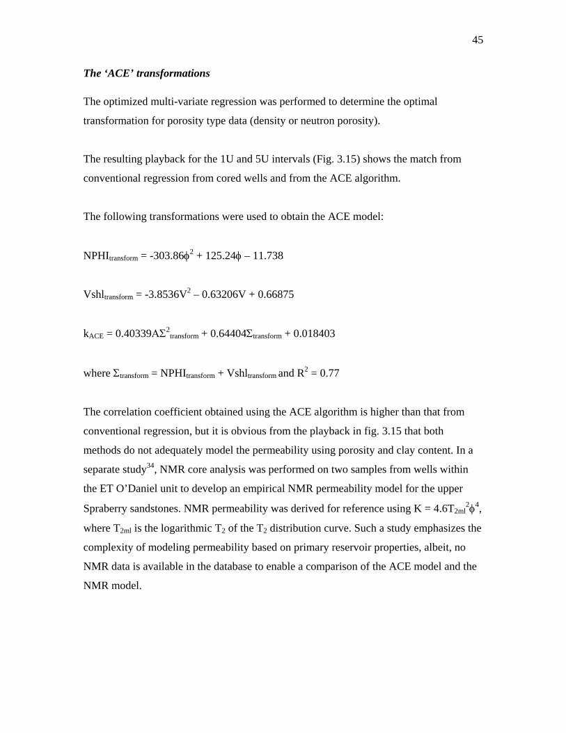
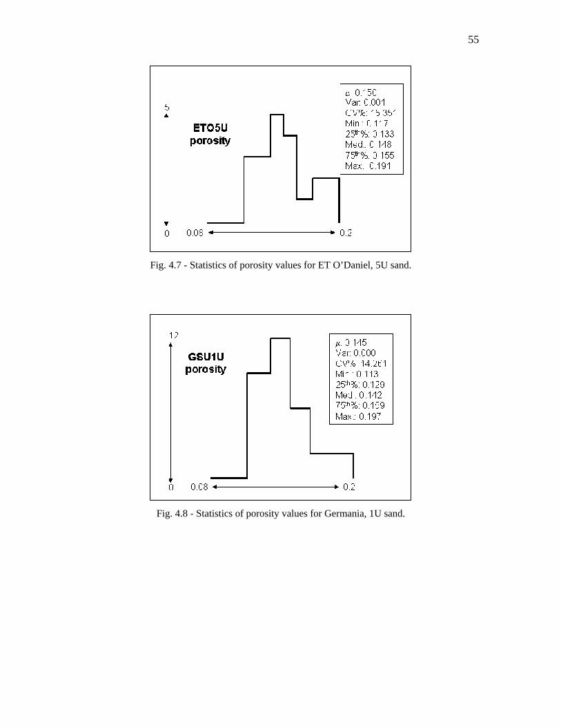
Fig. 4.7 - Statistics of porosity values for ET O’Daniel, 5U sand.
Fig. 4.8 - Statistics of porosity values for Germania, 1U sand.

56
Fig. 4.9 - Statistics of porosity values for Germania, 5U sand.
Kolmogorov – Smirnov test for porosity and shale volume
This test is based on measuring the maximum vertical separation between two empirical
CDF’s36 given as dmax. This method makes it possible to compare entire distributions
rather than any single statistical measure.
For a one sided test at the 5% confidence level, the value of 1.36(I1I2)0.5(I1+I2)0.5 must
exceed I1I2dmax for the two empirical distribution forms to be considered the same.
Sample size for data set 1, I1 = 31
Sample size for data set 2, I2 = 22
Critical value not to be exceeded is given by I1I2dmax, and the test value is given by
1.36(I1I2)0.5(I1+I2)0.5. From Fig. 4.10, the value of dmax is given by the maximum vertical
distance between the two functions.
Resulting values are 47.06 and 258 respectively, this indicates that the distributions are
somewhat different. A limitation37 of this test is that it is more sensitive close to the

57
center of the distribution, than at the tail, evidenced by the Fig. 4.10 where dmax occurs
about the center.
Fig. 4.10 – Kolmogorov - Smirnov test on porosity function, 1U sand.
Results of other comparisons between the units of ET O’Daniel and Germania for
porosity and shale volume are summarized in table 4.1 below.
A further limitation in the value of any inference as a result of a comparative analysis of
Germania and ET O’Daniel lies in the sample size. The ET O’Daniel dataset is about half
the size of the Germania dataset for shale volume, it is therefore a possibility that
improvement in correlations will be made as the database is expanded. See appendix B11

58
for illustration of effect of varying sample sizes on the Kolmogorov – Smirnov test for a
normal distribution.
Table 4.1 – Kolmogorov-Smirnov test for porosity and shale volume.
I1 I2 dmax Critical TestPorosity 1U 31 22 6.90% 47.06 258.56Porosity 5U 31 20 10.60% 65.72 241.84
Vshl 1U 50 23 7.10% 81.65 394.05Vshl 5U 50 21 6.00% 63.00 371.33
Litho- stratigraphic section
Another factor that lends itself to the verification of the ET O’Daniel and Germania units
being analogous to one another is the depositional continuity over the two fields.
The 1U and 5U sands as well as the over and underlying intervals are well defined in
both fields, and are at approximately the same depth horizons, and most of all, are picked
by all the wells analyzed. Similar depositional characteristics are also observed i.e.
prominent shale markers and fining/coarsening sand trends.
Figs. 4.11 and 4.12 show gross thickness map of both fields with line of section (A-A’)
indicated and the litho-stratigraphic section displaying the 5 sand units in the upper
Spraberry.

59
Fig. 4.11 – Gross thickness map of the 1U sand.
(Section A-A’ along the north–south dip wise axis of the Spraberry trend area).
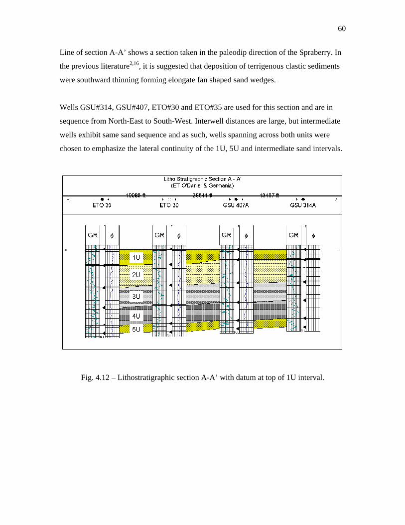
60
Line of section A-A’ shows a section taken in the paleodip direction of the Spraberry. In
the previous literature2,16, it is suggested that deposition of terrigenous clastic sediments
were southward thinning forming elongate fan shaped sand wedges.
Wells GSU#314, GSU#407, ETO#30 and ETO#35 are used for this section and are in
sequence from North-East to South-West. Interwell distances are large, but intermediate
wells exhibit same sand sequence and as such, wells spanning across both units were
chosen to emphasize the lateral continuity of the 1U, 5U and intermediate sand intervals.
Fig. 4.12 – Lithostratigraphic section A-A’ with datum at top of 1U interval.

61
CHAPTER V
MODEL APPLICATION IN GERMANIA UNIT
Germania
Picks and interval properties
The Germania unit shows through the gamma ray logs, the characteristic response
observed in the ET O’Daniel unit within the five reservoir units (1U thru 5U). The
formation markers were generally distinguishable and continuous over the lateral space
between both units. Application of the log based rock model to distinguish reservoir and
non-reservoir quality rock through porosity and shale indicators will form the basis of the
reservoir description process and the generation of structure and isopach maps that
describe this unit.
Fig. 5.1 – Payzone prediction based on rock model for GSU146A, 1U sand.
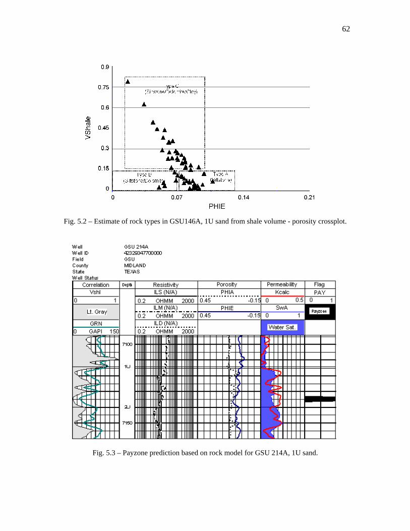
62
Fig. 5.2 – Estimate of rock types in GSU146A, 1U sand from shale volume - porosity crossplot.
Fig. 5.3 – Payzone prediction based on rock model for GSU 214A, 1U sand.
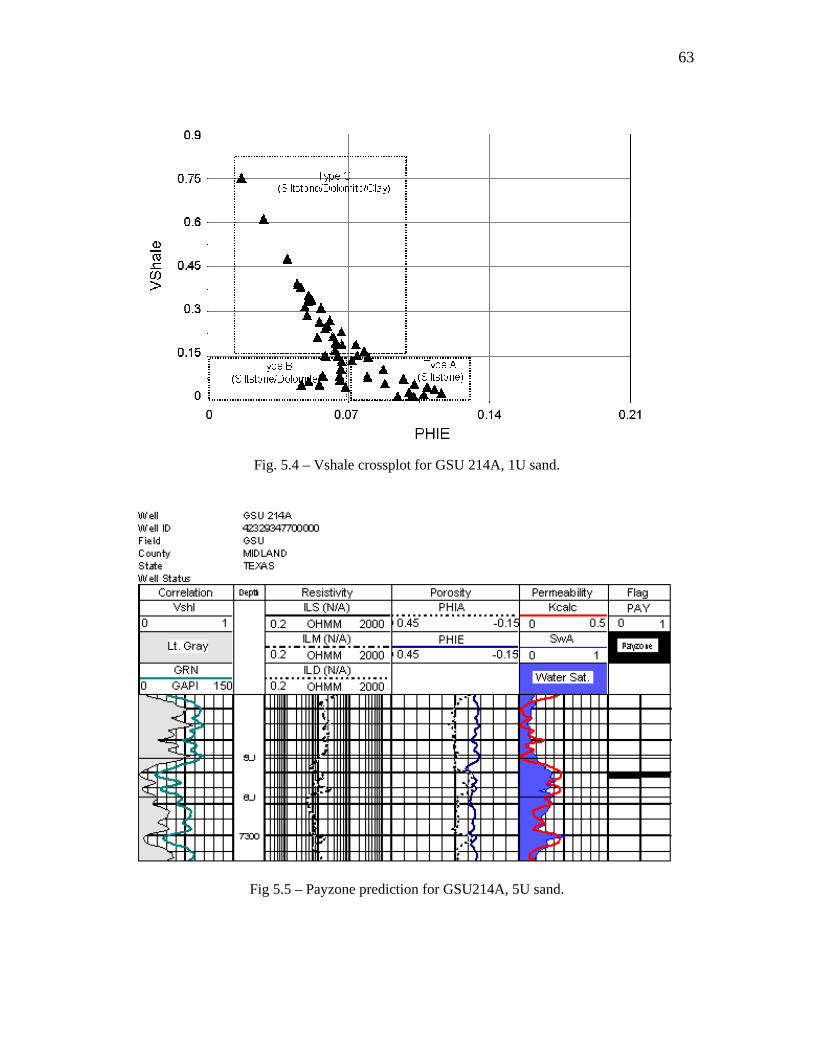
63
Fig. 5.4 – Vshale crossplot for GSU 214A, 1U sand.
Fig 5.5 – Payzone prediction for GSU214A, 5U sand.

64
Fig. 5.6 – Vshale crossplot for GSU 214A, 5U sand.
The log based rock model developed from log analysis and petrographic studies in the ET
O’Daniel unit, was applied with partial success in the Germania Spraberry unit. From
observation within the GSU log playback, the rock model consistently underestimated the
pay interval compared with the average ET O’Daniel interval.
Figs. 5.1 to 5.6 provide a visual means of quantifying the net sand with respect to the
gross sand thickness. It is evident that the net to gross sand ratio drastically reduces based
on the rock – log model estimates in the Germania unit with respect to the ET O’Daniel
prediction estimates.
The 1U sand shows a net to gross ratio of about 30% as compared to 50% in the ET
O’Daniel unit. A dissimilar trend is also observed, in that the low clay sands are not
exclusively rock type A, but are mostly type B – dolomitic siltstone. In the 5U unit, the
net to gross ratio observed here is about 20% compared to the 40% observed in the
equivalent ET O’Daniel unit.
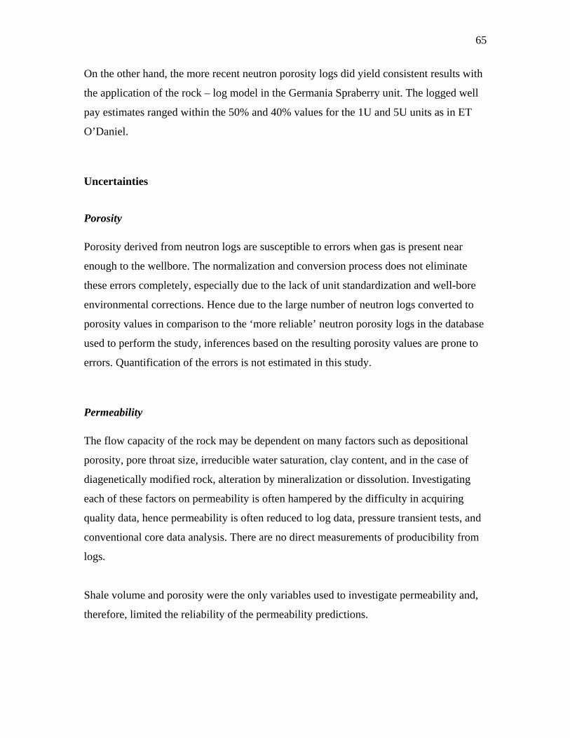
65
On the other hand, the more recent neutron porosity logs did yield consistent results with
the application of the rock – log model in the Germania Spraberry unit. The logged well
pay estimates ranged within the 50% and 40% values for the 1U and 5U units as in ET
O’Daniel.
Uncertainties
Porosity
Porosity derived from neutron logs are susceptible to errors when gas is present near
enough to the wellbore. The normalization and conversion process does not eliminate
these errors completely, especially due to the lack of unit standardization and well-bore
environmental corrections. Hence due to the large number of neutron logs converted to
porosity values in comparison to the ‘more reliable’ neutron porosity logs in the database
used to perform the study, inferences based on the resulting porosity values are prone to
errors. Quantification of the errors is not estimated in this study.
Permeability
The flow capacity of the rock may be dependent on many factors such as depositional
porosity, pore throat size, irreducible water saturation, clay content, and in the case of
diagenetically modified rock, alteration by mineralization or dissolution. Investigating
each of these factors on permeability is often hampered by the difficulty in acquiring
quality data, hence permeability is often reduced to log data, pressure transient tests, and
conventional core data analysis. There are no direct measurements of producibility from
logs.
Shale volume and porosity were the only variables used to investigate permeability and,
therefore, limited the reliability of the permeability predictions.

66
Water saturation
An inverse approach was used in determining saturations, and as is often the case, there is
non-uniqueness in the defining parameters. In this case, the Archie parameters have pre-
established tolerances as shown in chapter II, but nevertheless different combination of
Archie parameters within this tolerance may still yield consistent matches from well to
well.
Net pay
Due to the limitations in the porosity predictions earlier mentioned, the rock log model
which is based on porosity and shale volume will equally be subject to errors. Therefore,
even though tried and tested, the rock log model may fail to adequately predict the
location and thickness of productive sub units.
67
CHAPTER VI
CONCLUSIONS
Electrofacies patterns within the ET O’Daniel are easily recognizable in the Germania
Spraberry unit and this correlation is evident across the units of the upper Spraberry. The
general reservoir structure is consistent across both unit and thus becomes the essence of
the Germania unit characterization.
Studies in the analog unit - ET O’Daniel, provided valuable input towards the
characterization effort of the Germania for a variety of reasons, the most fundamental
being the log based rock model used for rock type discrimination.
The simplicity of the model makes it easy to use as a criteria for determining pay quality
within the upper Spraberry, once the correlatable units are identified. Secondly, the core
analysis performed by Reservoirs Incorporated enabled the development of porosity and
permeability relationships that may be applied in the GSU, the result of which are
porosity and permeability maps to guide further development and simulation studies.
Conclusions
1. The Isopach maps indicate channel deposits and interdistributary flat features that
are consistent with the depositional evaluation proposed by Handford et al. The
facies indicate detrital clasts of both depositional episodes as evident in the
lithology charts in chapter II which indicate that the 1U and 5U intervals are made
up of terrigenous sandstones as well as dolomitic carbonate facies.
2. Particularly evident in the ET O’Daniel Isopach maps are the north - south
thinning of the sandstone intervals, this is indicative of an energy source north of
the Spraberry.

68
3. The Germania unit isopach (net thickness) is conservative in its estimation of net
pay thickness, this is can be attributed to the limitations of the log based rock
model in predicting payzones based on normalized cased hole neutron logs.
Neutron logs alone do not lend themselves to corrections (environmental etc).
Porosity correction techniques require a multi-dimensional array of porosity data
i.e. density and neutron or sonic. Ideally, the density and neutron porosity logging
devices should be run together so as to allow for necessary compensatory
corrections in log data.
4. Optimal non-parametric regression techniques did not clearly improve the
estimations of permeability based on shale volume and porosity. The method in
itself is efficient, but alternative or more appropriate relationships specific to the
Spraberry units need to be investigated. Additional studies on pore throat
distribution based on core analysis may offer opportunities to improve the
predictions.
5. Techniques for determining water saturation in the spraberry or shaly sands do not
recommend using the Archie’s equation. The Archie model is simplistic in its
approach and is only considered a means of ‘estimating’ water saturation for this
study.
6. Acquisition of core data within the Germania unit is not an option. To enable
further evaluation of the GSU, core derived parameters must be available to guide
simulation studies and inform fracture characterization to yield an integrated
reservoir model.

69
REFERENCES
1. Schechter, D.S., McDonald, P., Sheffield, T., and Baker, R.: “Reservoir
Characterization and CO2 pilot Design in the Naturally Fractured Spraberry
Trend” paper SPE 35469 presented at the 1996 Permian Basin Oil and Gas
Conference, Midland, 27-29 March.
2. Handford, C.R.: “Sedimentology and Genetic Stratigraphy of Dean and Spraberry
Formations (Permian), Midland Basin, Texas” AAPG Bulletin (1981), 65, no. 9,
1602.
3. Barfield, E.C., Jordan, J.K., and Moore, W.D.: “An Analysis of Large-Scale
Flooding in the Fractured Spraberry Trend Area Reservoir” JPT (1959), 11, 15.
4. Schechter, D.S.: “Advanced Reservoir Characterization and Evaluation of CO2
Gravity Drainage in the Naturally Fractured Spraberry Trend Area” 2nd Annual
Technical Progress Report, US DOE Contract No. DE-FC22-95BC14942,
Socorro, New Mexico (August 1997).
5. Schechter, D.S.: “Advanced Reservoir Characterization and Evaluation of CO2
Gravity Drainage in the Naturally Fractured Spraberry Trend Area” 1st Annual
Technical Progress Report, US DOE Contract No. DE-FC22-95BC14942,
Socorro, New Mexico (August 1996).
6. McDonald, P., Lorenz, J.C., Sizemore C., Schechter, D.S., and Sheffield, T.:
“Fracture Characterization Based on Oriented Core from the Spraberry Trend
Reservoir: A Case Study” paper SPE 38664 presented at the 1997 SPE Annual
Technical Conference and Exhibition, San Antonio, 5-8 October.

70
7. Reservoirs Inc.: “Geological and Petrophysical Analysis of the Upper Spraberry
Formation, Midland County, Texas” Report prepared for Parker & Parsley
Development Co., Midland, Texas (1997), 1 & 2.
8. Schechter, D.S., and Banik; A.S.: “Characterization of the Naturally Fractured
Spraberry Trend Shaly Sands Based on Core and Log Data” paper SPE 35224
presented at the 1996 Permian Basin Oil and Gas Conference, Midland, 27-29
March.
9. Schechter, D.S., and Banik; A.S.: “Integration of Petrophysical and Geologic Data
with Open-Hole Logs for Identification of the Naturally Fractured Spraberry
Payzones” paper SPE 38913 presented at the 1997 SPE Annual Technical
Conference and Exhibition, San Antonio, 5-8 October.
10. Mardock, E.S., and Myers, J.P.: “Radioactivity Logs Define Lithology in the
Spraberry Formation” Oil and Gas Journal (Nov. 1951), 90.
11. Lyttle, W.J., and Rieke, R.R.: “Well Logging in the Spraberry” Oil and Gas
Journal (Dec. 51), 92
12. Schechter, D.S., and Putra, E.: “CO2 Pilot Design and Water Injection
Performance in the Naturally Fractured Spraberry Trend Area, West Texas” paper
SPE 71605 presented at the 2001 SPE Annual Technical Conference and
Exhibition, New Orleans, Sept. 30-Oct. 3.
13. Putra, E.: “Reservoir Simulation of Waterflood Pilot in Naturally Fractured
Spraberry Trend” paper SPE 54336 presented at the 1999 Asia Pacific Oil and
Gas Conference and Exhibition, Jakarta, 20-22 April.
14. Schechter, D.S., and Buoyun, Guo .: “An Integrated Investigation for Design of a
CO2 Pilot in the Naturally Fractured Spraberry Trend Area, West Texas” paper

71
SPE 39881 presented at the 1998 International Petroleum Conference and
Exhibition, Villahermosa, 3-5 March.
15. Wilkinson, W.M.: “Fracturing in Spraberry Reservoir, West Texas” AAPG
Bulletin, (Feb 1953), 37, no. 2, 253.
16. Schmitt, G.T.: “Genesis and Depositional History of Spraberry Formation,
Midland Texas” AAPG Bulletin (Sept. 1954), 38, no. 9, 1957
17. Tyler, N., and Gholston, J.C.: “Heterogeneous Deep Sea Fan Reservoirs,
Shackelford and Preston Waterflood Units, Spraberry Trend West Texas”
University of Texas at Austin Bureau of Economic Geology, Report of
Investigations (1998), 171, 38
18. Montgomery, S.L., Schechter, D.S., and Lorenz, J.: “Advanced Reservoir
Characterization to Evaluate CO2 flooding, Spraberry Trend, Midland Basin,
Texas” AAPG Bulletin (2000), 84, no. 9, 1247.
19. Asquith, G.B.: Log Analysis of Shaly Sandstone Reservoirs: A Practical Guide,
AAPG (1992), Tulsa Oklahoma
20. Greder, H.N., Mus, E.A., Veillerette, A.M., Pellerin, and F.M.: “Derivation of a
Core Permeability Log and Extrapolation to Uncored Intervals” Proc. 36th
Society of Professional Well Log Analyst Symposium (1995), 12p.
21. Balan, B., Mohaghegh, S., Ameri, S.: “State-of-the-Art in Permeability
Determination from Well Log Data: Part I- A Comparative Study Model
Development” paper SPE 30978 presented at the 1995 Eastern Regional
Conference and Exhibition, Morgantown, 17-21 September.

72
22. Allen, J.R.: “Prediction of Permeability from Logs by Multiple Regression”
Trans. 36th SPWLA Symposium (1995)
23. Van Den Bosch, R., Fulop, A., and, Pistre, V.: “Permeability Prediction from
Well Logs – A Case Study in German Rotliegend Sandstones” Trans. 36th
SPWLA Symposium (1995), 12p.
24. Hook, J.R., Nieto, J.A., Kalkomey, C.T., and Ellis, D.: “Facies and Permeability
Prediction from Wireline Logs and Core – A North Sea Case Study” Trans. 35th
SPWLA Symposium (1994), AAA1.
25. Saxena, V.: “Hydrocarbon Evaluation through Modulus Decomposition of Sonic
Velocities in Shaly Sands” Trans. 37th SPWLA Symposium (1996), 14p.
26. Breiman, L., and Friedman, J.H.: “Estimating Optimal Transformations for
Multiple Regression and Correlations” Journal of the American Statistical
Association (1985), 80, 580.
27. Guoping Xue, Datta-Gupta, A., Valko, P., and Blasingame, T.: “Optimal
Transformations for Multiple Regression: Application to Permeability Estimation
from Well Logs” paper SPE 35412 presented at the 1996 Improved Oil Recovery
Symposium, Tulsa, 21 April.
28. Shier, D.E., Course Notes for Well Log Normalization Work Shop, Published
privately by Energy Data Services, Golden, Colorado (1991).
29. Crain, E.R., Garrido, M.:“Qualitative Analysis of Older Rocks for Porosity and
Permeability – Lake Maracaibo, Western Flank Reservoirs, Venezuela” Petroleos
de Venezuela (PDVSA)
73
30. Hunt, E., Aly, A., and Pursell, D.: “Fundamentals of Log Analysis, Part 6,
Determining Basic Log Analysis Parameters - a, m, n, and Rw” World Oil, (Oct.
1996), 217, no.12, 59
31. Neinast, G. S., and Knox, C. C.: “Normalization of Well Log Data” Trans. 14th
SPWLA Symposium (1973), I1.
32. Isaaks, E.H., and Srivastava, R.M.: An Introduction to Applied Geostatistics,
Oxford University Press (1989).
33. Hunt, E., and Pursell, D.: “Fundamentals of Log Analysis, Part 7, Determining
Shaliness from Logs” World Oil, (1996), 218, no.3, 55
34. Reservoirs Inc.: “NMR Core Analysis: Upper Spraberry Formation, ET O’Daniel
Lease Area, Midland County, Texas” Report prepared for Parker and Parsley
Development Co., Midland, Texas (1997)
35. Rasmus J.C.: “Variable Cementation Exponent, m, for Fractured Carbonates” The
Log Analyst (1983), 41.
36. Jensen J.L., Lake L.W., Corbett P.W., and Goggin D.J.: Statistics for Petroleum
Engineers and Geoscientists, Prentice Hall (1997)
37. NIST/SEMATECH e-Handbook of Statistical Methods,
http://www.itl.nist.gov/div898/handbook/
38. Gibson, G.: “The Relation of Fractures to the Accumulation of Oil in the
Spraberry Formation” Proc. 3rd Oil Recovery Conference, West Texas Petroleum
Research Committee, Bulletin 15 (1951), 16.
39. Ogden, V., and Locke, J.: “Core Data Discussions” ibid., Bulletin 15, 57.

74
40. Marshall, J.W.: “Spraberry Reservoirs of West Texas” Geological Notes (1952),
2189.
41. Lang, W.H., Jr.: “Porosity Log Calibrations” The Log Analyst (1980), 21, no. 2,
14.
42. Shier, D.E.: “A Comparison of Log Response between Logging Companies and
Different Vintages of Tools” The Log Analyst (1997), 38, no. 3, 47.
43. Shier, D.E., and Sponable, D.M.: “Correcting Drift in GNT Neutron Log Data
from West Texas” The Log Analyst (1997), 38, no. 3, 16.
44. Hardle, W.: Applied Non-parametric Regression, Cambridge University Press,
Cambridge (1990)
45. Reservoir Inc.: “Geological and Petrophysical Analysis of the Upper Spraberry
Formation in Midland County, Texas” Report prepared for Parker and Parsley
Development Co., Midland, Texas (1996)
46. Jensen, J.L., and Lake, L.W.: “Optimization of Regression Based Porosity
Permeability Predictions” presented at the 1985 10th Canadian Well Logging
Society, Calgary
47. Boardman, D.W. et al.: “Use of Effective Properties for Characterization of a
Naturally Fractured Reservoir in East Venezuela” paper SPE 53881 presented at
the 1999 Latin American and Caribbean Petroleum Engineering Conference,
Caracas, 21-23 April.
48. Guevara, E.H.: “Geologic Characterization of Permian Submarine Fan Reservoirs
of the Driver Waterflood Unit, Spraberry Trend, Midland Basin, Texas”

75
University of Texas at Austin Bureau of Economic Geology, Report of
Investigations (1988), no. 172, 44p.
49. Asquith, G.B.: “The Importance of Determining Pore Type from Petrophysical
Logs in the Evaluation of a Permian Wolfcamp Reentry, Northern Midland
Basin” The Log Analyst (1997), 38, no. 3, 37.
50. Ingerman V.G.: “Statistical Integration of Log Data for Lithology Determination
and Formation Evaluation” The Log Analyst (1995), 36, 38.
51. Katahara, K.W.: “Gamma Ray Log Response in Shaly Sands” The Log Analyst
(1995), 36, 50.
52. Gamboa, P., Reis, J., and Morris, S.: “Development of a Log Based Petrophysical
Model for a Complex Dolomite Reservoir” The Log Analyst (1994), 35, 47.
53. Whatler, P.: “Core Data Quality Issues” The Log Analyst (1994), 35, 43.
54. Nelson, P.H.: “Porosity - Permeability Relationships in Sedimentary Rocks” The
Log Analyst (1994), 35, 38.

76
APPENDIX A
BACKGROUND GEOLOGY AND STRATIGRAPHY
Geology/Geophysical Background
The Spraberry trend area spans an area about 150 miles in length and 50 miles at the
broadest width, and has been found to be productive in an area approximately 500,000
acres16. The trend is estimated to originally contain over 8.5 billion barrels of oil of which
only 8 – 12% have been recovered thus far. Structural contours show that the Spraberry
trend lies updip and to the east of current day Basinal axis, which exists adjacent to the
central Basin platform (Figure A1).
Regional Stratigraphy and Lithofacies
The Midland Basin is known to be composed of largely of shallow – marine shelf to shelf
margin carbonates, as well as deep Basin deposits2. Early opinions were that the Dean
and Spraberry formations were wolfcampian in age, Silver and Todd2 reported based on
biostratigraphic and physical stratigraphic evidence that the formations are Leonardian in
age.
Stratigraphic sections analyzed by Jeary2 suggest that the Spraberry formation
Leonardian in age and is coeval with the upper and middle Clearfork and Glorieta
formations (Figures A2 and A3), these correlations become less obvious in other areas of
the Basin due to discontinuity of clastic strata across shelf margins and well control
reasons.
The Spraberry formation is approximately 1000ft thick and is generally composed of
852ft of black shale and silty shale, 131ft of siltstones and 5ft of thin bedded limestones
or dolomites. This formation belongs to the lower Leonard and rests conformably on the
Wolfcamp. The black fissile shales and thin dolomite beds of the Clearfork group which
directly overlies the Spraberry are fractured similar to the Spraberry rocks and with the
same lithologic appearance.

77
The mass of the Spraberry can be separated into 3 distinct and correlative units, which are
classified as the upper, middle and lower Spraberry with each unit of approximately the
same thickness. The texture and mineralogical character of the major constituents can be
described based on rock types as follows:
Siltstones ~ Major percentage of grains fall within the silt size range (< 1/16 mm), with
about 60% between the grade limits of 0.03mm – 0.06mm. Grains range from angular
Fig. A1 - Structure contour data, top of Spraberry sandstone, Midland Basin, west Texas18.

78
Fig. A2 - Regional geologic setting of Permian Basin, west Texas2.
to very angular and the sorting is from fair to poor. Primarily, the cementing agent is
dolomite with some silica.
Dolomites ~ Vary in texture from fine to crystalline, the fine crystals being primary.
Shales ~ Several types of shales have been encountered, massive blocky as well as the
commonly found fissile brittle type. Most of the shales have been classified as

79
carbonaceous, but in all petrographic slides examined, the shales were found to be silty
and ferruginous.
Fig. A3 - West – east stratigraphic cross section BB’2.
(Note shelf-to-Basin correlations and informally identified stratigraphic units 4 and 5. See Fig.
A2 for location).

80
Characteristics of the lithofacies are found to be areally and vertically consistent as
observed from all the wells examined. Distinctions can be made from electric logs
between the upper, middle, and lower Spraberry, however there is no easily apparent
characteristic that differentiates the clastic content in the three units from one another,
when observed by petrographic microscope. This provides a useful means of recognizing
three sandstone-siltstone lithofacies based on bedding characteristics:
- Massive to Parallel and cross laminated sandstone and siltstone.
- Laminated Sandstone and siltstone
- Bioturbated sandstone and siltstone
Gamma-Ray logs can often distinguish lithofacies. Laminated and Bioturbated siltstones
having a greater shale content than parallel and cross laminated sandstones and siltstones
respond with a more radioactive curve.
A Lithofacies map (Fig. A4) of the four County area (Upton, Reagan, Midland and
Glasscock) substantiates the geological features at the close of the Wolfcamp time. The
northeast of the Spraberry trend non clastics are dominant with a gradual facies change
toward the productive area, where approximately 87% of the Spraberry is shale. West of
the producing area a rather abrupt shale to limestone facies change occurs, with several
wells on the west side of the present day structural highs containing 85% of non-clastics.
The interpretation being that during the time of Spraberry deposition, the west side of the
Midland Basin was elevated sufficiently to provide an environment of warm shallow
waters, in which carbonates were precipitated and deposited. Superimposed on the
lithofacies map are isopach contours representing the thickness of Spraberry type rocks
after total deposition and after accounting for all structural movement.

81
Fig. A4 - Lithofacies map, four County area with Spraberry isopach contours15.
Depositional Model
The Spraberry formation was deposited by debris flow, turbidity currents, saline density
currents and suspension settling. Some sediments were later altered by slumping, soft
sediment faulting, and fluidization. Deep Basin carbonate members were largely
deposited by debris flow, turbidity, saline and density currents, while deposition of
terrigenous clastics was dominated by turbidity, saline and density currents, and

82
suspension settling. Thus clastic and carbonate members shared the same deep-marine
setting and most depositional processes. However, the exclusive occurrence of saline
density-current deposits within the terrigenous clastic facies indicate that large frequently
tapped reservoirs of dense saline waters were stored in shelf lagoons or salt pans near the
shelf margin, but only during times of clastic deposition on the shelf.
The fundamental part of any Spraberry model (Figs. A5 – A7) must recognize major
alternating periods of carbonate and clastic deposition, incorporate the principal attributes
of the carbonate and clastic patterns, and show how styles interacted to form the observed
stratigraphic framework2.
Fig. A5 – Facies model of clastic and carbonate dominated shelf margin systems2.

83
Fig. A6 – Distribution of environments, geometry of deposits, and channel patterns2.
Fig. A7 – Sections of onlapping clastics and downdip widening of channels2.
(Sections AA’ and BB’ from fig. A6)

84
During carbonate depositional episodes (Fig. A5) which characterized the northern shelf
margin in early and late Clear Fork time, calcareous organisms flourished. A massive
carbonate shelf margin (1,700 – 2,000 ft) above the floor of the adjacent midland Basin,
prograded Basinward over resedimented carbonate debris forming the slope. Slumps
debris flow and turbidity currents were the principal mechanisms by which carbonate
sediments were moved downslope into the Basin.
During Tubb and Glorieta times, large influx of silt and mud caused mud rich sabkhas
and salt pan environments to prograde rapidly across the southern Palo Duro Basin
towards the shelf margin of the Midland Basin, giving rise to clastic depositional
episodes (Fig. A5). Sub tidal to inter tidal sand sheets accumulated at the shelf margin,
from which silt and sand were periodically carried into the Basin by saline density
currents that drained hypersaline shelf lagoons and salt pans.
Deposition of terrigenous-clastics sediments formed southward thinning, elongate fan
shaped wedges (Fig. A6). Sandstone and siltstone were deposited principally from
density underflow and interflow currents. Deposition from bottom hugging currents
formed elongate patterns which branch and rejoin in updip regions and bifurcate in
downdip regions.
Clastic Patterns
The total sand and silt found in the upper Spraberry decreases from north to south.
During upper Spraberry time, areas in the northeastern part of the Midland Basin
subsided more rapidly and received a thicker sequence of sand and silt. Around the edges
of the Basin a gradual decrease is noted in the total net thickness of the sand and silt in
the direction of the shelf areas. The rate of decrease is more rapid in the northern part of
the Basin where there is thicker development of the coarse clastics (Fig. A8). Within the
four County area (Midland, Glasscock, Upton and Reagan), the thickness is nearly
constant.

85
Fig. A8 – Isopach map of upper Spraberry unit in Midland County16.
Clastic ratio – Determined by the total thickness of the clastics (sand, shale, silt) at any
control point divided by the total thickness of non-clastics (limestone, dolomite). Data is
based on sample and electric log study (Fig. A9). Over a wide area in the central part of
the Basin, the clastic ratio is greater than 8 (more than 88% of the section is composed of
clastics). The width of this zone decreases north and south. Another slight decrease in the

86
clastic ratio occurs around the edge of the more negative area developed in northeastern
Gaines County. Where the section is thinner there may have been a better development of
carbonates. Possibly carbonates were deposited as rapidly around the edges as in the
central part, but the central part subsided more rapidly and received a thicker sequence of
clastics. Along the northeastern edge the decrease in clastics was, in part, due to the thick
Pennsylvanian and Wolfcampian reefs16.
Fig. A9 – Clastic ratio map of upper Spraberry unit in Midland County16.

87
Flow Units
The Spraberry is divided into 3 main intervals (Upper, Middle and Lower), Tyler &
Gholston further sub-divided the Spraberry into distinct episodes or operational units. Of
the six units found in the upper Spraberry, only two (1U and 5U) are reservoir quality
rock, while in the lower Spraberry only two operational units are identified. Little is
known about the lower Spraberry formation, as focus is mostly on the upper Spraberry.
Fig. A10 - Operational units within the upper Spraberry formation.
(TXL Fee ‘B’ #1 well located in the central trend area).
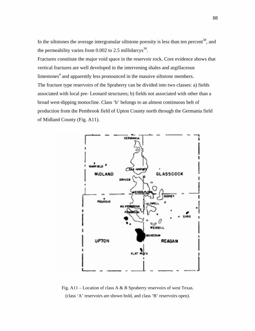
88
In the siltstones the average intergranular siltstone porosity is less than ten percent38, and
the permeability varies from 0.002 to 2.5 millidarcys39.
Fractures constitute the major void space in the reservoir rock. Core evidence shows that
vertical fractures are well developed in the intervening shales and argillaceous
limestones4 and apparently less pronounced in the massive siltstone members.
The fracture type reservoirs of the Spraberry can be divided into two classes: a) fields
associated with local pre- Leonard structures; b) fields not associated with other than a
broad west-dipping monocline. Class ‘b’ belongs to an almost continuous belt of
production from the Pembrook field of Upton County north through the Germania field
of Midland County (Fig. A11).
Fig. A11 – Location of class A & B Spraberry reservoirs of west Texas.
(class ‘A’ reservoirs are shown bold, and class ‘B’ reservoirs open).

89
APPENDIX B
MAPS FOR ET O’DANIEL AND GERMANIA
Fig. B1 - Minimum gamma ray map of ET O’Daniel, 5U sand.

90
Fig. B2 - Maximum gamma ray map of ET O’Daniel, 5U sand.

91
Fig. B3 - Paleo-structure map of ET O’Daniel, 1U sand.

92
Fig. B4 - Paleo-structure map of ET O’Daniel, 5U sand.

93
Fig. B5 - Paleo-structure map of Germania, 1U sand.

94
Fig. B6 - Paleo-structure map of Germania, 5U sand.
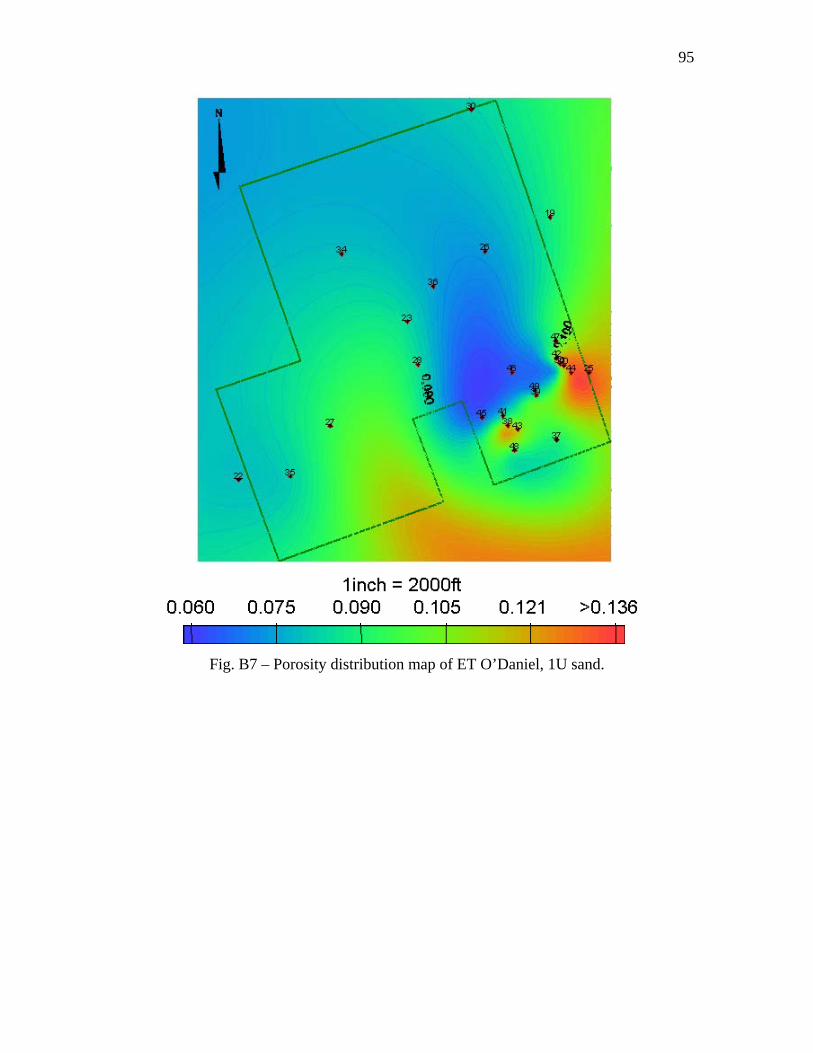
95
Fig. B7 – Porosity distribution map of ET O’Daniel, 1U sand.

96
Fig. B8 - Porosity distribution map of ET O’Daniel, 5U sand.

97
Fig. B9 – Porosity distribution map of Germania, 1U sand.
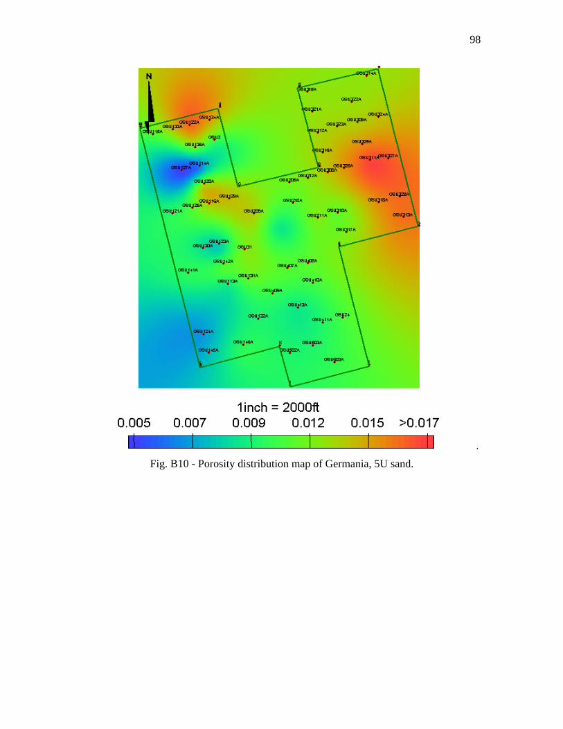
98
.
Fig. B10 - Porosity distribution map of Germania, 5U sand.

99
Fig. B11 – Effect of sample sizes on Kolmogorov –Smirnov distribution test.

100
VITA
Babajide Adelekan Olumide
Education
B.Sc. Industrial Engineering U. of Ibadan, Nigeria Sept. 1993
High School: International School, U. of Ibadan, Nigeria Sept. 1987
Work Experience
6/99 to 7/01 Texaco Overseas Pet. Co. Nigeria Unlimited
Responsibilities: Senior Drilling Engineer
6/97 to 6/99 Texaco Overseas Pet. Co. Nigeria Unlimited
Responsibilities: Drilling Supervisor
9/94 to 6/97 Texaco Overseas Pet. Co. Nigeria Unlimited
Responsibilities: Drilling Engineer
Permanent Address
c/o Joseph Taiwo
19618 Riverbottom Road
Katy, TX 77449