charles university in prague - cuni.cz
TRANSCRIPT

Charles University in Prague
Faculty of Social SciencesInstitute of Economic Studies
BACHELOR THESIS
Patents: Means to Innovation orStrategic Ends?
Author: Martin Stepanek
Supervisor: PhDr. Jirı Schwarz
Academic Year: 2011/2012

Declaration of Authorship
The author hereby declares that he compiled this thesis independently, using
only the listed resources and literature. The author also declares that he has
not used this thesis to acquire another academic degree.
The author grants to Charles University permission to reproduce and to dis-
tribute copies of this thesis document in whole or in part.
Prague, May 15, 2012 Signature

Acknowledgments
I am most thankful to PhDr. Jirı Schwarz, my thesis supervisor, for his relent-
less support, great ideas, and occasional commendation. The responsibility for
all errors is mine.
I would also like to thank PhDr. Jana Votapkova for her consultation about
the Data Envelopment Analysis.

Abstract
This paper utilizes an extensive dataset of 163,663 US patents granted between
1976 and 2011 to 25 companies within four technological fields (aerospace in-
dustry, computer manufacturing, semiconductor industry, and software devel-
opment), to observe fluctuations in their value and characteristics. I find that
certain indicators have changed immensely during the last 36 years, suggesting
that newer patents are much less valuable than their predecessors. Further,
using Data Envelopment Analysis, I estimate relative production efficiency of
transformation of inputs (research and development expenses and company’s
workforce) into outputs (patent stock and its technological importance), to
provide an empirical evidence for the recent theories of strategical patent ex-
ploitation by large companies. I find that the efficiency varies considerably for
different industries and also for the companies within an industry. There is an
overall trend of increasing efficiency in patent production per unit of input, but
there is none in the effectiveness of creating valuable inventions, which seems
to depend only on the company itself.
JEL Classification D22,L20,O32,O34
Keywords patent value, intellectual property rights, strate-
gic patents, research and development efficiency
Author’s e-mail [email protected]

Abstrakt
Tato prace vyuzıva rozsaheho souboru dat o 163 663 americkych patentech
25 spolecnostı ze ctyr technologickych odvetvı (letectvı, pocıtacova technika,
polovodice a softwarove inzenyrstvı) mezi roky 1976 a 2011, ke sledovanı zmen
v jejich hodnote a vlastnostech. Podle mych pozorovanı se nektere ukaza-
tele velmi vyrazne zmenily v prubehu poslednıch 36 let, coz naznacuje, ze
novejsı patenty jsou vyrazne mene cenne nez jejich predchudci. Dale, s vyuzitım
Data Envelopment Analysis, odhaduji relativnı efektivnost, se kterou mnou po-
zorovane firmy premenujı vstupy (vydaje na vyzkum a vyvoj, pocet zamestnan-
cu) na vystupy (pocet patentu a jejich technologicka hodnota), abych obo-
hatil nedavnou teorii o strategickem zneuzitı patentu firmami. Zjistil jsem, ze
tato efektivita je rozdılna nejen pro ruzna odvetvı, ale i pro firmy v danych
odvetvıch. Ukazalo se, ze efektivita tvorby patentu jako takovych vzrostla,
nicmene efektivita v tvorbe technologicky vyznamnych vynalezu zalezı pouze
na dane firme.
JEL klasifikace D22,L20,O32,O34
Klıcova slova hodnota patentu, dusevnı vlastnistvı, strate-
gicky patent, efektivita vyzkumu a vyvoje
E-mail autora [email protected]
Rozsah prace 97 682 znaku (vcetne mezer)

Contents
List of Tables viii
List of Figures ix
Acronyms x
Thesis Proposal xi
1 Introduction 1
2 Strategical Patents 4
3 Patent Valuation 7
3.1 Patent Indicators . . . . . . . . . . . . . . . . . . . . . . . . . . 9
3.2 Correlates of Patent Value . . . . . . . . . . . . . . . . . . . . . 12
3.2.1 Used Variables . . . . . . . . . . . . . . . . . . . . . . . 14
4 The Dataset 17
5 Descriptive Statistics 20
5.1 Citations . . . . . . . . . . . . . . . . . . . . . . . . . . . . . . . 20
5.2 Family Size . . . . . . . . . . . . . . . . . . . . . . . . . . . . . 27
5.3 Renewals . . . . . . . . . . . . . . . . . . . . . . . . . . . . . . . 28
5.4 Patent Trades . . . . . . . . . . . . . . . . . . . . . . . . . . . . 30
5.5 The Other Variables . . . . . . . . . . . . . . . . . . . . . . . . 31
6 Empirical analysis 33
6.1 Econometric analysis . . . . . . . . . . . . . . . . . . . . . . . . 33
6.2 DEA analysis . . . . . . . . . . . . . . . . . . . . . . . . . . . . 39
7 Conclusion 47

Contents vii
Bibliography 54
A Forward Citation Distribution I
B Data download VI
C Additional Figures and Tables VII
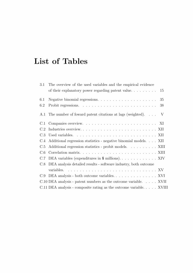
List of Tables
3.1 The overview of the used variables and the empirical evidence
of their explanatory power regarding patent value. . . . . . . . . 15
6.1 Negative binomial regressions. . . . . . . . . . . . . . . . . . . . 35
6.2 Probit regressions. . . . . . . . . . . . . . . . . . . . . . . . . . 38
A.1 The number of foward patent citations at lags (weighted). . . . V
C.1 Companies overview. . . . . . . . . . . . . . . . . . . . . . . . . XI
C.2 Industries overview. . . . . . . . . . . . . . . . . . . . . . . . . . XII
C.3 Used variables. . . . . . . . . . . . . . . . . . . . . . . . . . . . XII
C.4 Additional regression statistics - negative binomial models. . . . XII
C.5 Additional regression statistics - probit models. . . . . . . . . . XIII
C.6 Correlation matrix. . . . . . . . . . . . . . . . . . . . . . . . . . XIII
C.7 DEA variables (expenditures in $ millions). . . . . . . . . . . . . XIV
C.8 DEA analysis detailed results - software industry, both outcome
variables. . . . . . . . . . . . . . . . . . . . . . . . . . . . . . . XV
C.9 DEA analysis - both outcome variables. . . . . . . . . . . . . . . XVI
C.10 DEA analysis - patent numbers as the outcome variable. . . . . XVII
C.11 DEA analysis - composite rating as the outcome variable. . . . . XVIII
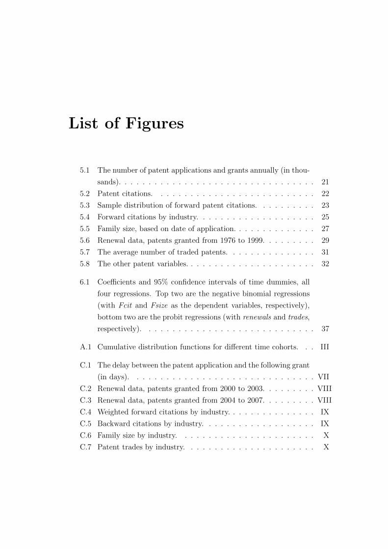
List of Figures
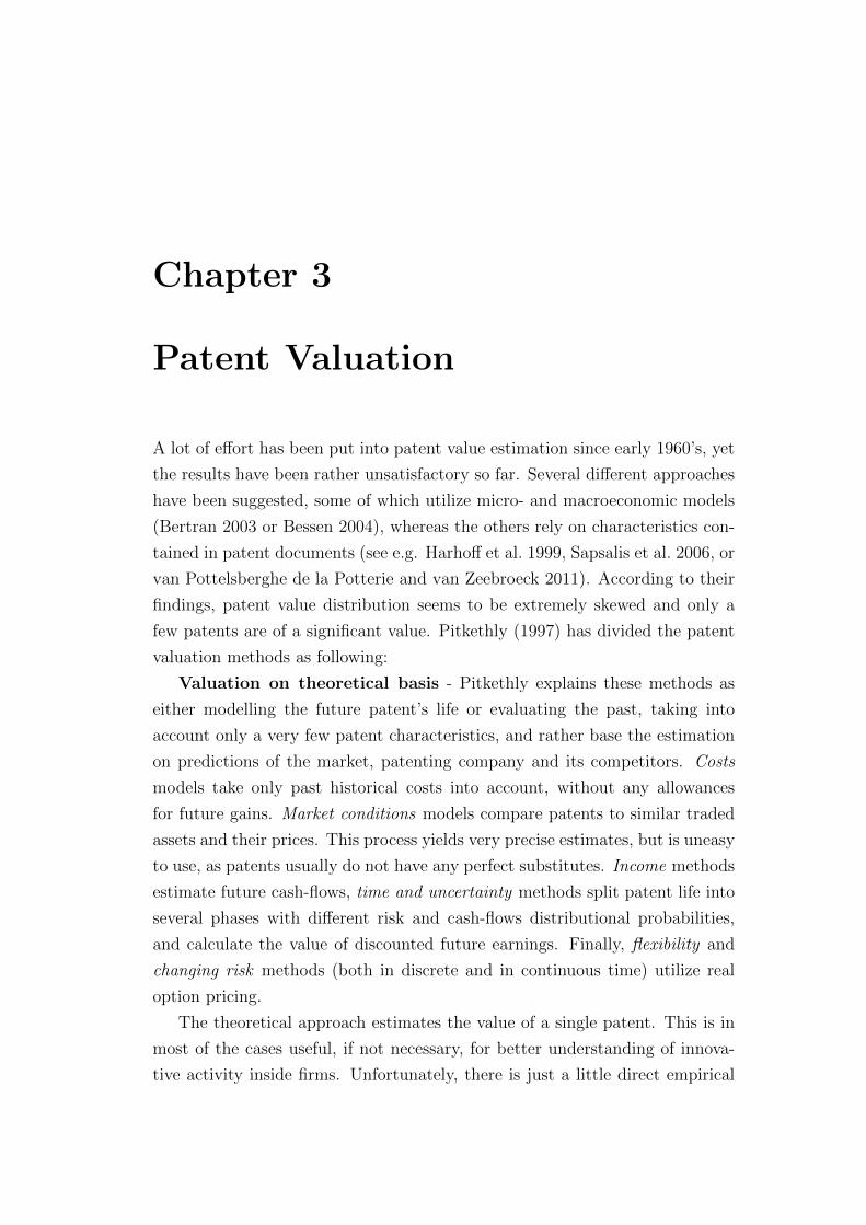
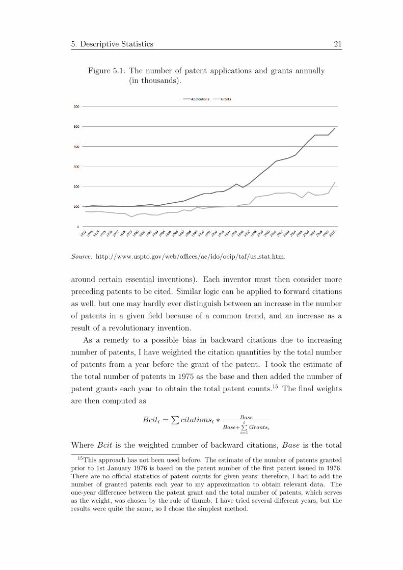
5.1 The number of patent applications and grants annually (in thou-
sands). . . . . . . . . . . . . . . . . . . . . . . . . . . . . . . . . 21
5.2 Patent citations. . . . . . . . . . . . . . . . . . . . . . . . . . . 22
5.3 Sample distribution of forward patent citations. . . . . . . . . . 23
5.4 Forward citations by industry. . . . . . . . . . . . . . . . . . . . 25
5.5 Family size, based on date of application. . . . . . . . . . . . . . 27
5.6 Renewal data, patents granted from 1976 to 1999. . . . . . . . . 29
5.7 The average number of traded patents. . . . . . . . . . . . . . . 31
5.8 The other patent variables. . . . . . . . . . . . . . . . . . . . . . 32
6.1 Coefficients and 95% confidence intervals of time dummies, all
four regressions. Top two are the negative binomial regressions
(with Fcit and Fsize as the dependent variables, respectively),
bottom two are the probit regressions (with renewals and trades,
respectively). . . . . . . . . . . . . . . . . . . . . . . . . . . . . 37
A.1 Cumulative distribution functions for different time cohorts. . . III
C.1 The delay between the patent application and the following grant
(in days). . . . . . . . . . . . . . . . . . . . . . . . . . . . . . . VII
C.2 Renewal data, patents granted from 2000 to 2003. . . . . . . . . VIII
C.3 Renewal data, patents granted from 2004 to 2007. . . . . . . . . VIII
C.4 Weighted forward citations by industry. . . . . . . . . . . . . . . IX
C.5 Backward citations by industry. . . . . . . . . . . . . . . . . . . IX
C.6 Family size by industry. . . . . . . . . . . . . . . . . . . . . . . X
C.7 Patent trades by industry. . . . . . . . . . . . . . . . . . . . . . X

Acronyms
DEA Data Envelopment Analysis
DMU Decision Making Unit
USPTO United States Patent Office
EPO European Patent Office
WIPO World Intellectual Property Organization
IPC International Patent Classification
AMD Advanced Micro Devices
AM Applied Materials
CS Citrix Systems
HP Hewlett-Packard
IBM International Business Machines
LTC Linear Technology Corporation
MIP Maxim Integrated Products
NC Nuance Communication
UT United Technologies

Bachelor Thesis Proposal
Author Martin Stepanek
Supervisor PhDr. Jirı Schwarz
Proposed Topic Patents: Means to Innovation or Strategic Ends?
Griliches (1981) provides empirical evidence that company’s patent stock
has a positive effect on its market value, particularly when accounting for num-
ber of references of other patents to analyzed patents (Hall, B.H., Jaffe, A.,
Trajtenberg, M., 2000). Harhoff et al. (2003) have shown that other aspects
of patents, such as patent scope or family size are correlated with the patent
value as well.
Those studies only investigate patent’s explanatory power of company’s
value as they are means of innovation, however, as Macdonald (2004) has
shown, patent can also be understood as a strategic instrument. A strate-
gic patent is only important as a tool to keep the company competitive among
others, not a mean of innovation. In my study, I will provide empirical analysis
from this point of view, using patent value as a measurement of innovativeness
of the patent.
Patent value can be understood as the market value of a patent (i.e. costs
for a company if it wanted to purchase a patent from another one) or as the
technological value (i.e. in means of innovation it brings). I will focus mainly
on the technological value which is shown to be correlated with e.g. family
size of the patent, patent scope or number of forward and backward references
related to the patent. I will show that the variables mentioned above, expenses
on research and development and other factors can be used to explain changes
in market value of a firm.
Assuming that higher value patents are the innovative ones and lower value
patents play the strategic role, I will test whether the value of firm’s patents has
changed over time. That is, whether strategic patents indeed are a phenomenon
of the recent years or if there has been no significant change in the average value
Bachelor Thesis Proposal xii
of the patents. The dataset will be constructed using a web crawler created for
this purpose, which will download the required data from the official website
of United States Patent and Trademark Office and related databases with free
access (particularly patents.google.com and www.freepatentsonline.com).
Outline
1. Introduction
2. Relationships among used variables
3. Model overview
4. Data Envelopment Analysis and auxiliary regressions
5. Testing hypotheses
6. Conclusion and future research
Core bibliography
1. Griliches, Z. (1981): Market Value, R&D and Patents. Economics letters. 7(2): pp.
183–187.
2. Hall, B.H., Jaffe, A., Trajtenberg, M. (2000): “Market Value and Patent Citations: A
First Look. NBER, Cambridge, MA
3. Harhoff, D., Scherer, F., Vopel, K. (2003): Citations, family size, opposition and the
value of patent rights. Research Policy. 32(8): pp. 1343–1363.
4. Macdonald, S. (2004): When means become ends: Considering the impact of patent
strategy on innovation. Information Economics and Policy. 16(1): pp. 135–158.
5. Pakes, A. (1985): On patents, R & D, and the stock market rate of return. The
Journal of Political Economy. 93(2): pp. 390–409.
6. Pitkethly, R. H. (1997): The Valuation of Patents: A Review of Patent Valuation
Methods with Consideration of Option Based Methods and the Potential for Further
Research. Judge Institute Working Paper. WP(21/97)
7. Reitzig, M. (2003): What do Patent Indicators Really Measure? A Structural Test of
‘Novelty’ and ‘Inventive Step’ as Determinants of Patent Profitability. LEFIC Center
for Law and Economics at the Copenhagen Business School.
8. Reitzig, M. (2004): Improving patent valuations for management purposes – validating
new indicators by analyzing application rationales. Research Policy. 33: pp. 939–957.
Author Supervisor

Chapter 1
Introduction
Innovative activity is the process of creating inventions. The inventor has to be
rewarded for that kind of activity, so the argument goes, as it generally increases
social welfare, and there would be suboptimal level of the activity without a
possible reward. State protection for the invention is an indirect form of such
a reward, and patenting is its possible mean. A patent is essentially a way of
possessing an invention, allowing to have similar rights as if it were a tangible
asset. The invention may then not be stolen or abused, and it may yield an
income from fees, should someone invent a new creation based on the patented
idea.
The history of patents goes back to the 15th century, but the idea of re-
warding inventors has been here from the time of ancient Greece (Devaiah,
undated). There are two extreme points of view at patenting; positive and
negative. The positive assumes that there would be no incentive for innovation
without patent protection, as it would not bring any reward. Yet there are
e.g. amateur writers, who do not seek a legal protection for their work and
thus prove that such institution is not a necessary condition for a creative ac-
tivity. The negative point of view highlights the fact that patents only create
an incentive for innovative activity; however, it may not result in a valuable
invention.
Nowadays, the process of innovation is mostly performed by the research
and development (R&D) sections of companies, not by individual inventors.
There are billions of dollars spent each year, and many companies hold portfo-
lios containing thousands of patents. Thanks to those, they can restrict their
competitors both on the market and in the race for technological lead. Bertran
(2003) argues that firms can nowadays target a given level of technological

1. Introduction 2
improvement and reach it in a given time, as they have routinized R&D. In
rapidly innovating industries, such as chemicals, drugs, computing equipment,
communication equipment, and professional and scientific instruments, is R&D
done with a much higher intensity, for the firm to keep competitive advantage
(Pakes and Griliches 1980). Smaller firms rely more heavily on trade secrets
than patents for protection of their ideas (Baldwin 1996), yet they have better
results in producing patents per $1 (Bound et al. 1982). Many economists have
tried to use patents and their characteristics as a measurement of the innova-
tive activity within firms (see e.g. Schmookler and Brownlee 1962 or Griliches
1990), or to link them to company’s performance (Griliches 1981, Hall et al.
2000, etc.).
Recently, a new phenomenon of strategic meaning of patents has been dis-
cussed by several authors (Yiannaka and Fulton 2006). While some companies
admit that they apply for new patents mostly for strategic purposes (Bessen
2004), the overall trend remains unclear. I will focus on this very interesting
behaviour and provide an empirical analysis to support the otherwise purely
theoretical literature.
I utilize a large dataset of US patents to show a change in the patent in-
dicators and statistics, as suggested by Jaffe and Lerner (2006). My peerless
dataset contains patents between 1976 and 2011 (the longest possible period to
be monitored due to a limited content of the patent office databases), whereas
the other recent studies (see e.g. Sapsalis and de la Potterie 2007 or Gam-
bardella et al. 2008) only observe patents from a short time span. Hence, I
provide a valuable contribution to the existing research. Then, combining and
further developing methods used by van Pottelsberghe de la Potterie and van
Zeebroeck (2011), van Zeebroeck (2011), Sapsalis et al. (2006), Sapsalis and
de la Potterie (2007), and other authors, I perform an econometric analysis to
show differences between my and the prior findings. Finally, I utilize Data En-
velopment Analysis, a method developed by Charnes et al. (1978), to measure
relative efficiency of the observed companies regarding transformation of in-
puts (R&D expenditures and company’s workforce) into outputs (patent stock
and its value). I find substantial distinctions not only among the companies,
but also throughout the observed time period. The results correspond to the
existing theories of strategical patents.
This paper is structured as follows: the next chapter presents a review of
the strategical meaning and use of patents, Chapter 3 provides an insight into
the history and different approaches to patent valuation, with focus on econo-

1. Introduction 3
metric analysis that I build upon later. Chapter 4 shows a summary of patent
indicators, Chapter 5 is devoted to the dataset, its descriptive statistics are
then depicted in Chapter 6. Chapter 7 covers the empirical analysis. Finally,
the last chapter concludes the work.

Chapter 2
Strategical Patents
Historically, the reason for requesting a patent protection had been the concern
about having own inventions being abused by a third party. Many companies
did not even see patenting as necessary, and it was more profitable for whole
technological fields to be mutually discrete and to not break other’s rights,
than to pay fees for patent application. Innovation had used to be an essential
process in obtaining a lead time on the market, resulting in company’s higher
earnings. However, this has changed dramatically in the beginning of the 20th
century, when the US patent offices significantly lowered required standards of
patent applications. Consequently, it has become much easier for a company to
make an application in order to obtain a patent grant. But, arguably, it has also
made the newly issued patents much less valuable at the same time, because
even inventions which would have never been granted patent protection before,
for their lack of novelty, became easily patentable. A decrease in singularity of
patents had led to a decline in patenting activity until 1982, when the Court of
Appeals for the Federal Circuit was set up. It was the first patent specialized
court in the USA. It upheld twice as many (up to 89%) lesser court decisions
that patents were valid than before, which significantly rose the value of US
patents; thus, it has again become favourable for companies to apply for them.
The sudden impact on the whole patent system was immense, patent grants in
the USA increased by 78% without a rise in research investment between 1983
and 1995 (Kortum and Lerner 1999).
Some industries, like pharmaceutics, have always supported the patent sys-
tem because of the nature of their products and impossibility to produce similar
products without breaching other’s rights. In these technological fields, a com-
pany may become a monopoly with a single invention; its competitors may
2. Strategical Patents 5
simply not be able to produce a substitute to its product. However, in other
fields, like semiconductor industry, the technology pace have always been much
faster than the process of patenting, which resulted in almost no patenting
activity during the 20th century. But, since 1982, companies have appreciated
every employee whose idea could be patented more than ever, and have decided
to continually patent their inventions as they would have fallen behind the com-
petition otherwise. Patents were kept and firms have continued in application
processes in all but the most worthless cases, no matter what industry they
competed in (Macdonald 2004).
The enormous increase in patent applications was not followed by an ade-
quate enlargement of patent offices. There were just too few employees without
advanced computer technology to deal with the immense amounts of applica-
tions.1 It has again led to even lower patenting standards, as there was not
enough time to carefully examine each request. It has been proved that the
worsening of patenting standards has resulted in a different management of
patent portfolios and an aggressive assertion of patents (Bessen 2004). Patents
no longer needed to carry any significant invention in order to be valuable
for the company through the competitive advantage they posed. Companies
started to aim for patent thickets instead of valuable innovations. A patent
thicket refers to complex products stretching over whole patent portfolios. This
is in a high contrast with the one-to-one correspondence between products and
patents usual before (i.e. the process of product creation only involves use of
one patent). A thicket is created around a key patent of a company, and in-
cludes both the patents of the company in possession of the key patent, and its
competitors. Having a patent in a thicket around the key patents held by the
competitor has become one of the new strategies that sprung up. The com-
petitor is then unable to fully utilize his own inventions, because his product
would involve a patent in a possession of a third party, most likely a competitor.
Moreover, such strategies may even end up preventing companies from selling
their products on certain markets.2
As (Hall and Ham 1999, pg. 10) put it,“The reasons that patents were
1Patents must go through several stages of examination, and the examiners may requestthe application form to be filled in due to some components missing or being improperlyprepared. The length of the whole process has changed substantially over the years, asshown in Figure C.1.
2In 2011, a court in Dusseldorf has forbidden Samsung to sell its tablet in Germany,upon a request from Apple. Just recently, in April 2012, another German court bannedMicrosoft from selling Xbox 360, Windows 7, Windows Media Player and Internet Explorerfor infringement of Motorola’s patent rights.

2. Strategical Patents 6
important often had little to do with whether patents provide an incentive to
conduct R&D or enable the firm to profit from the generation of products on
which the invention was based”. The more difficult it becomes to circumnav-
igate the protected invention with a new technology, the more valuable the
patented invention is for a company willing to block its competitors. Gallini
(2002) has shown that the greater is the breadth of patent protection (i.e. the
more areas the patent is involved in), the harder it is for other companies
to break into the market with their own innovations, without violating the
patented protection and thus breaking the law, and the longer the company
can maintain the limited monopoly. Bessen (2004) proved that, under general
conditions, firms attempting for cross-licensing (i.e. creating patent thickets)
have lower incentives for R&D. Such firm’s patent portfolio is then intertwined
with its competitor’s; thereby, every accomplishment producing profits is then
only shared through licensing.3 He also showed that mutually non-aggressive
strategies lead to higher social welfare. Other strategies, as listed in Macdonald
(2004), include: patent discoveries that might block use of similar discoveries
in competitors’ products, or to patent in order to have a portfolio with which
to negotiate licensing agreements with other companies.
So far the literature dealing with strategical patents has only shown the
theoretical background of why it would be more profitable for a company to
not aim at creation of valuable inventions, but to be involved in patent thickets
instead. One way how to observe such behaviour empirically is to analyse
changes in patent production. Simple patent counts would not be sufficient
though, as those are highly correlated with R&D expenses and the size of a
firm. Therefore, I take advantage of DEA to see the change in efficiency of
production, rather than to analyse the volume of the output. Yet not only the
analysis itself is important; the descriptive statistics of my extensive dataset
illustrate a lot of these changes as well.
In order to be able to successfully accomplish these tasks, one must first
have a deeper understanding of patent valuation and characteristics. The next
chapter introduces the main concepts.
3In the dispute between Motorola and Microsoft, Motorola wants 2.25% of the salesprice for using its inventions (O’Gara 2012). Many large companies nowadays must makeagreements with their competitors, in order to be even able to produce (e.g. Apple andSamsung, companies which otherwise sue each other, have an agreement for Samsung creatingsemiconductor parts for Iphone, without which would Apple not be able to make it.)
Chapter 3
Patent Valuation
A lot of effort has been put into patent value estimation since early 1960’s, yet
the results have been rather unsatisfactory so far. Several different approaches
have been suggested, some of which utilize micro- and macroeconomic models
(Bertran 2003 or Bessen 2004), whereas the others rely on characteristics con-
tained in patent documents (see e.g. Harhoff et al. 1999, Sapsalis et al. 2006, or
van Pottelsberghe de la Potterie and van Zeebroeck 2011). According to their
findings, patent value distribution seems to be extremely skewed and only a
few patents are of a significant value. Pitkethly (1997) has divided the patent
valuation methods as following:
Valuation on theoretical basis - Pitkethly explains these methods as
either modelling the future patent’s life or evaluating the past, taking into
account only a very few patent characteristics, and rather base the estimation
on predictions of the market, patenting company and its competitors. Costs
models take only past historical costs into account, without any allowances
for future gains. Market conditions models compare patents to similar traded
assets and their prices. This process yields very precise estimates, but is uneasy
to use, as patents usually do not have any perfect substitutes. Income methods
estimate future cash-flows, time and uncertainty methods split patent life into
several phases with different risk and cash-flows distributional probabilities,
and calculate the value of discounted future earnings. Finally, flexibility and
changing risk methods (both in discrete and in continuous time) utilize real
option pricing.
The theoretical approach estimates the value of a single patent. This is in
most of the cases useful, if not necessary, for better understanding of innova-
tive activity inside firms. Unfortunately, there is just a little direct empirical

3. Patent Valuation 8
evidence from patent data to support it.
Econometric valuation methods estimate the impact of patent indica-
tors on patent value, taking advantage of accessibility of such variables in
large volumes. Some of the indicators are directly correlated with observable
prices, costs, sold quantities, or with latent variables such as novelty, inven-
tive step, breadth, and dependence on complementary assets, which have some
self-explanatory power and may be utilized for further research (Reitzig 2004).
The first attempts to evaluate patents using econometric analysis come from
Schmookler and Brownlee (1962), who searched for a relationship between the
number of patents in company’s portfolio and the total factor productivity.
They did not find any significant correlation. The main pioneer in the field
of econometric patent valuation was Zvi Griliches. In 1981, he observed a
relationship between firm’s output, employment, and physical and R&D capital
(Griliches 1981), followed by a discovery of a significant impact of R&D on
company’s value (Griliches 1984). A long effect of $1 spent on R&D adds $2 in
the market value of the firm above and beyond the indirect influence of patents.
Although, only unanticipated R&D expenditures seem to have a positive effect.
Pakes (1985) demonstrated that about 5% of the variance in the stock market
value of a firm is caused by events changing both R&D and patent applications.
Despite the importance of these earlier findings, the most crucial change
came with the data transformation into electronic form. Previously manually
unobtainable volumes of data led to discoveries of new relationships among
the patent characteristics and patent value. The recent works exhibit correla-
tion between patent indicators and the likelihood of litigation (Lanjouw and
Schankerman 1997, Lanjouw and Schankerman 2004), renewal decisions (van
Pottelsberghe de la Potterie and van Zeebroeck 2011), or e.g. differences be-
tween academic and industrial patents (Sapsalis et al. 2006). Nevertheless,
patent value and its extremely skewed distribution, however well it can be ob-
served, is far from being satisfactorily explained. Some authors have argued
that the distribution may conform rather well to the log-normal distribution.
Scherer (1998) in his work shows that the distribution of returns from inno-
vation may be less skewed than log-normal, but with a long log-linear tail.
In other words, there are a very few extremely valuable patents, producing
many times higher revenues than their actual costs through R&D, and an over-
whelming number of patents worth almost nothing. As (Pitkethly 1997, pg.
2) characterizes the issue, “patents are like lotteries in which there are a few
prizes and a great many blanks”.

3. Patent Valuation 9
Following van Pottelsberghe de la Potterie and van Zeebroeck (2011), the
generally used model is:
V aluei = f(PCi, OCi, Si)
where V aluei is the estimated value of patent i, PCi are patent characteristics
obtained from the application and grant documents, OCi are characteristics of
patent’s owner, and Si are the results of an inventor and owner survey. I will
characterize each of those more precisely in the following two sections.
3.1 Patent Indicators
Reitzig (2004) divided patent indicators obtainable from the application and
grant documents into three categories:
First generation variables are not related to a deeper knowledge of insti-
tutional background of the patent system, and thus are easy to be interpreted
and used. Nevertheless, they do not take depreciation into account. Those
include patent citations and family size of the patent.
Patent citations can be either forward or backward, and show the knowledge
flows among patents. A backward citation exhibits a relationship between two
particular patents; one being an underlying basis (the cited patent) for another
one (the citing patent). Patentee who seeks for state protection of his idea
must first create a list of patents and non-patent literature upon which he has
built the new invention. As the patent is applied for, it goes through many
stages of examination, where the examiner inspects the correctness of such
lists and searches for more possible preceding patents or literature. The grant
document then includes both the citations from the examiner and from the
inventor himself. Reitzig (2003a) argues that backward citations to previously
issued patents may exhibit market potential, whereas citations to non-patent
literature ought to indicate greater technological value. The knowledge flows,
assumed to be shown by patent citations, are supposed to be only present if
the citation comes from the inventor, not the examiner (Alcacer and Gittelman
2006). Jaffe et al. (2000) made a survey on inventors and found out that they
were fully aware of less than one-third of the backward citations of their patents.
Alcacer and Gittelman (2006) then confirmed the observation and showed that
about 63% of backward citations come from examiners, 40% of all patents only
contain backward citations from examiners, and there are only 8% of patents
that were needless of adding any citations from the examiner.
3. Patent Valuation 10
There is a large difference in backward citation counts when comparing
patents under the US (USPTO) and European (EPO) patent offices. European
patents show spectacularly low numbers of citations. It might be because there
are less inventions patented in Europe than in the USA - the patents have
less options to which to refer. The second possible explanation is a different
approach of USPTO. The application for a patent protection must satisfy ’best-
mode practice’; a full list of patents that could possibly be considered a prior
art has to be made as a part of patent application. In Europe, the majority
of citations come from the examiner, not the applicant (Harhoff et al. 1999).
The large difference in citation counts is one of the reasons why it is difficult
to compare studies analysing the European patents to those analysing the US
patents.
The crucial aspect of backward citations is their immediate availability at
the date of the patent grant. The list of backward citations doesn’t change
throughout patent’s life, and thus is a very reliable as a value indicator. Sev-
eral successful attempts were made to show a relationship between backward
citations and patent value, and indeed observed a positive correlation (see e.g.
Narin et al. 1997).
The creation of backward citations naturally implies the existence of their
opposites - forward citations (citations received from other patents). Those
also show the knowledge flows; however, there is a significant difference in the
meaning. Backward citations do not necessarily prove the newly issued patent
to bring any kind of novelty, they only show a relationship to the underlying
invention. But a gain of a forward citation shows a direct impact of the patent
on the other inventions. A patent without a gain of a forward citation after a
few years is most likely an unimportant one, at least as far the technological im-
provement is concerned. On the other hand, a patent with numerous citations
from the other inventions should be of a significant technological value.
Forward citations also have several drawbacks. First, a possible bias may
occur in the estimation if a company cites its own patents. Some authors argue
that such behaviour may demonstrate creation of patent thickets around com-
pany’s invention (Bessen 2008). Second, the most important difficulty arises
from the nature of forward citations; the number of forward citations can grow
over patent’s life. The list of forward citations is always empty at the begin-
ning. US patents are validated for up to 20 years, and even then there is still
a possibility a patent may receive another forward citation in the future. This
probability is lower in certain technological fields (e.g. semiconductor industry)

3. Patent Valuation 11
as a result of rapid innovation. Uncertain citation counts pose a major difficulty
for any statistical or econometric analysis using patents from different years.
Hall et al. (2000) made an assumption that the lifetime of a patent is not longer
than 35 years. Bertran (2003) showed that they were quite right, and moreover
proved that the distribution of received citations barely changes after 12 years
since the application date. Further, Hall et al. (2000) exposed that more than
80% of all citations received by patents occur within the first 17 years after
the grant. Works of Albert et al. (1991), Lanjouw and Schankerman (2001), or
Harhoff et al. (2003) show a positive and very significant correlation between
forward citations and patent value. However similar results these works ex-
hibit, they are very different at the same time, mostly because they build their
observations upon dissimilar datasets. For my study, I have predicted the total
number of forward citations a patent would obtain 31 years after the grant (see
Chapter 5).
The last indicator in the first category is patent’s family size (Lanjouw and
Schankerman 2001, or Harhoff and Reitzig 2004). A company may seek for a
patent protection for one invention in more countries. Patents related to the
same invention, issued in different states, create a patent family. This variable
should in theory be positively correlated with patent value due to additional
costs connected with the patent application, renewal and possible litigation. A
company should only seek for such protection for its most valuable patents (as-
suming that its management board has the information advantage over general
public, leading it through the decision-tree). The works of Harhoff and Reitzig
(2004) confirmed the theory and found a rather strong correlation. Reitzig
(2003b) argues that patent’s family size should be a measure of market size of
the patent. Family size data are available soon after the patent application,
see Chapter 6 for further discussion.
More indicators usable as explanatory variables became available with the
introduction of improved patent databases on the internet. The second gen-
eration indicators include international and local patent classifications.
Patent classifications refer to the scope of a patent. In other words, the
number of different technological areas a patent is involved in. Patent scope
should be correlated with patent value since more valuable inventions would
serve as a foundation for innovation in different technological fields. Never-
theless, the newly developed patent strategies may require patents to have as
wide scope as possible to create even more powerful thickets at the same time.
The effect of a broader breadth on the value of a patent is then unclear, be-

3. Patent Valuation 12
cause strategical breadth is not linked to technological value. Indeed, Lerner
(1994), Harhoff and Reitzig (2004), and several other authors observed great
differences in the connection of patent classifications to patent value.
There are several different types of patent classifications. I am most inter-
ested in the US, European and International ones. International classification
(IPC) divides technological fields into eight sections with approximately 70,000
subdivisions. Each subdivision has a symbol consisting of Arabic numerals and
letters of the Latin alphabet. The IPC symbols are allotted by the national or
regional industrial property office that publishes the patent document.4 US and
European classifications are quite similar to IPC. Lerner (1994) argues that IPC
reflects the economic importance of new inventions, whereas US classification
focuses on the technical meaning.
The last category includes third generation indicators, among which Re-
itzig (2003b) puts variables that come from the patent full-text documentation,
such as the number of claims, design of certain text passages in the patent draft,
the number of words describing the state of the art, or the number of indepen-
dent claims.
Patent claims are the very essence of the invention itself. One can learn
how to make and use it from the description, yet only patent claims define the
scope of the legal protection. It is then a concern of every applicant to provide
the broadest possible patent claim to have the most sufficient protection as
a reward for his invention. Nevertheless, even the patentee must consider his
claims very well, as there is an increasing probability of litigation against the
issued patent when the claims are broader. It has been shown that the number
of words in the description has no explanatory power, whereas the number of
claims is very significant Reitzig (2003a). Recently, van Pottelsberghe de la
Potterie and van Zeebroeck (2011) found an important relationship between
the strategies of application filling and patent value.
3.2 Correlates of Patent Value
Because patent value is an abstract term without a precise definition, it has
to be substituted by its correlate. With the new discoveries, different variables
have been used as they seemed to have a better explanatory power regarding
patent value.
4http://www.wipo.int/classifications/ipc/en/general/preface.html

3. Patent Valuation 13
The most accurate method of estimation of patent value seems to be a
survey made on the inventors and their managers, i.e. the best informed peo-
ple regarding their inventions, who also further decide about patent’s validity.
Harhoff et al. (1999) or Gambardella et al. (2008) made such a survey, Gam-
bardella sent a questionnaire to inventors, questioning: ”Suppose that on the
day on which this patent was granted, the applicant had all the information
about the value of the patent that is available today. In case a patent com-
petitor of the applicant was interested in buying the patent, what would be the
minimum price the applicant should demand?”, asking them to put the value of
a given patent into one of 10 categories, starting at “less than e 50,000”, and
ending at “more than e 5,000,000”. They obtained very high estimates, with
mean value e 3,000,000 and median e 300,000. Harhoff et al. (1999) had very
similar results, 12.9% of patents in their survey were placed in the “more than
DM 5,000,000” category.
Another approach is to look at the record of patent renewal decisions. Cur-
rently, an utility patent in the USA can be validated up to 20 years, starting at
the filling date. The applicant has to pay maintenance fees in order to keep the
patent valid. In most of the European countries, these fees are paid annually,
whereas in the USA the fees are to be paid after 3.5 years, 7.5 years and 11.5
years. The fees grow rapidly over time and are different for small and large
firms (the charge is double for large companies). This approach utilizes the
imperfect information distribution; patent manager is ought to have sufficient
information about the invention to decide whether the possible gains from hav-
ing the invention protected are larger than the fee that has to be paid. Paying
the renewal fee gives him then not only the monopoly for the given time, but
also an option to pay another renewal fee when the time expires (Pitkethly
1997). The patentee needs to consider only the current renewal period for the
optimal decision, as the invention becomes more unprofitable with time due to
increasing fees (Bessen 2008).
The downside of this method is that patents can only be looked upon retro-
spectively and the results may be biased because patents may be renewed only
for strategical purposes, not because of their actual objective economical or
technological value. Rapid innovation in a whole industry may lower the value
of a given patent just after paying the fee as well. Arora et al. (2008) argues
that the renewal approach assumes the annual returns from having the patent
in force to decrease monotonically over patent’s life, and that patents may have
earned a lot in the first years even though they were not renewed. Further, the
3. Patent Valuation 14
estimates only show the extra value generated by issuing the patent, not the
value of an invention to firm if it were not protected by a patent. This is
different to the survey approach, which treats patents as assets, so the asking
price should reflect both the invention value and the patent premium. Hence,
it yields higher estimates than models only estimating the premium, such as
the renewal fee model.
Using renewal fee conception, Bessen (2008) indeed obtained much lower
estimates of patent value than Gambardella in his study. The mean value was
$78,168 and median only $7,175. He also found that patents owned by small
companies are less often renewed than those owned by larger ones. He puts it
as the patents of small companies are thus of a lower value, but it may simply
point out the propensity of larger companies to renew their patent portfolios,
for the cost is insignificant in comparison to the smaller companies.
The last major approach utilizes patent litigation. The probability a com-
pany would be sued for its invention increases with patent value (see Lanjouw
and Schankerman 2001, Reitzig 2003b, Harhoff and Reitzig 2004), as it is rather
costly for other firms to appeal to the court, thus only the most important (i.e.
valuable) patents should be opposed. The probability of a patent being liti-
gated increases with the number of companies inventing in the same area and
the number of claims of the patent (Lanjouw and Schankerman 1997). Reitzig
(2003b) created an litigation likelihood estimator for his econometric model and
used the patent indicators as explanatory variables to estimate the probability
of litigation. In his study, 11.5% of 16,711 European patents were opposed.
The oppositions were successful in 38% of cases.
Other correlates, like the market value of the firm or Tobin’s Q, have been
proposed; however, those can only be linked to the value of a whole patent
portfolio, not to single patents. Serrano (2005) recently came up with an idea
of connecting patent value to the probability that a patent would be traded
to a different company, arguing that the transfer of intellectual property has
become an important source of technology for firms. He showed that more
valuable patents are indeed more likely to be traded. I further utilize this very
interesting finding in my econometric analysis.
3.2.1 Used Variables
An important distinction must be made here; patent indicators, described in
Section 3.1 (except for forward citations), are contained in the patent document

3. Patent Valuation 15
and depend solely on the application process.5 The value correlates (including
forward citations), on the other hand, are given by personal decisions (e.g. to
renew a patent) and depend only on the importance of the patent (i.e. its
value).6
The preceding literature suggests a number of possible variables that may
stand as patent indicators or as value correlates. I follow and further develop
the method suggested by van Pottelsberghe de la Potterie and van Zeebroeck
(2011) and use variables that have previously been shown to have very signifi-
cant explanatory power regarding patent value, to obtain a composite variable
reflecting it. See Chapter 6 for its description.
Table 3.1: The overview of the used variables and the empirical evi-dence of their explanatory power regarding patent value.
Value Correlates Total Positive Negative Insignificant
Forward Citations 34 31 0 3Family Size 22 14 1 7Renewals 15 14 0 1Patent Trade 1 1 0 0
Patent IndicatorsInventors 4 1 1 2Backward patent citations 21 13 1 7Patent Classification 12 6 3 5Number of Inventors 5 1 2 2Priorities 2 0 0 2
Source: van Pottelsberghe de la Potterie and van Zeebroeck (2011)
Table 3.1 shows the complete list of the patent value correlates and the
patent indicators in my study, together with the number of distinct prior works
using them in econometric models, their significance, and sign. Three of my
patent value determinants (forward citations, renewal data and family size)
5All of these are known at the date of the patent grant. They only tell us patent specifi-cations, its breadth and the prior art the patent builds upon, but they cannot tell us muchabout the patent value without additional information. It is like a knowledge of the colour,engine capacity, and the number of doors of a car. We can see that it has more/less thanthe other cars, but can hardly say if it is better.
6Even under strategical behaviour, the assumptions should hold. Continuing the examplewith a car, these variables are similar to how high the car gets in consumer’s ranking, thedecision whether to buy the car, or the decision to later create a new model based on it.These latter variables may then be connected to the former ones (i.e. the decision whetherto buy a car may depend on its colour and engine volume.)

3. Patent Valuation 16
have been many times proved to be highly and positively correlated with patent
value (see e.g. Bessen 2008 or Reitzig 2003b), whereas patent trades have only
been used once so far. To support the theory that traded patents are more
valuable, I construct a model similar to the one used by Serrano (2005) to
obtain resembling results. Furthermore, I use these four variables for DEA
and provide a broad discussion of their evolution in Chapter 5. Finally, the
patent indicators have given ambiguous results so far, mostly due to different
explained variables they have been used with.7 I will use similar models to
those in the preceding literature to test how my data behave regarding the
value correlates I chose.
7Again, the colour of the car may be correlated with the purchase decision, but hardlywith the decision to further remake the car.

Chapter 4
The Dataset
The unique dataset I have created for my study contains data about 163,663
US patents from 4 technological industries: computer manufacturing, computer
software development, aerospace industry, and semiconductor industry, featur-
ing 25 companies in total. The data were downloaded from publicly accessible
patent office databases using web scraping program (for more information and
the full list of the observed companies see Appendix). I have selected those
industries because they are more innovative than the other (Griliches 1998).
On-line database of the NASDAQ Stock Market8 offers a roll of listed compa-
nies divided by industry. From those, I have picked only firms with market
value over $2 billion and history longer than 10 years. Listed companies are
generally obliged to publicly release their annual reports. Moreover, since 1994,
the US companies must post their fillings in electronic form. The reports can
be found in the Edgar-SEC database9 to obtain additional data. The condition
of market value above $2 billion and preferably a long history is required for
meaningful analysis. Smaller companies have patent portfolios of insufficient
size for statistical and econometric relevance, and it would be impossible to see
a shift in the patent strategy of a firm if it had just a short history. Of course,
the analysis for whole industries would be possible even when accounting for
the smaller firms, but the restriction had to be made at some point, since there
are also companies owning patents and not listed on a public stock exchange.
It would be nearly impossible to obtain a complete list of all relevant subjects,
so I made the limitation.
With the list of all suitable companies, I have searched the website of
8http://www.nasdaq.com9http://www.sec.gov/edgar.shtml

4. The Dataset 18
USPTO10 for their patents. Ultimately, I had a list of over 190.000 patents
of the firms, including various departments in different states. Unfortunately,
the US patent database (or any other free database) does not offer spreadsheet
or bulk downloads. In fact, they offer no explicit tool to download the data.
The method I used to obtain the dataset is depicted in the Appendix. I was able
to download the following characteristics: patent number, application number,
filling date, date of the grant, patent’s assignee, references cited (backward ci-
tations), US classification, International classification, and whether the patent
have been traded. However, due to incomplete database (missing data), the
final dataset must have been cleaned in order to have complete statistics.
Some of the observed companies own patents also from other than their main
industries. Because it is rather impossible to distinguish to which industry a
patent exactly belongs to, the trend should be common for all the companies
within an industry (i.e. companies from computer manufacturing most likely
also own several patents from software development or semiconductor industry,
aerospace companies may own computer patents etc.), and these patents ought
to form a small share of the patent portfolio of a given company, I treat all
the patents of one company as if they were from the industry in which I have
classified the company.
Additional data were found on the website of EPO.11 Those include: Euro-
pean classification, priority numbers, citing documents (forward citations), and
family size. Again, the data are only accessible in text format (and cannot be
easily downloaded), which creates certain difficulties in their use. Therefore,
the data had to be refined in several computer programs.
There are two other features impossible to be obtained from the patent
office databases: patent renewal and litigation data. Litigation data can only
be accessed through a very expensive private database, and are not included
in my work for that reason. Patent renewal data are available through Google
bulk download12 and may be downloaded without restrictions. Ultimately, I
have created a unique and extremely comprehensive dataset, containing patents
with date of the grant ranging from 1976 to 2011, and including characteristics
that have never been together before. About 30,000 (16%) records must have
been deleted due to missing data13 and patents of unrelated companies with
similar names to those on my list.
10http://www.uspto.gov11http://www.epo.org12http://www.google.com/googlebooks/uspto.html13Some characteristics (usually one, at most two variables per patent) were not present in

4. The Dataset 19
In the next section, I present the most interesting observations regarding
my dataset. While the preceding literature has mostly focused on looking for
the links between patent indicators, a little attention has been paid to the
evolution of the indicators themselves. I shed some light upon this matter to
contribute to the prior findings.
the database. I was unable to find any rule regarding the missing data, thus I assume it is arandom effect, which should not have any impact on my analysis.

Chapter 5
Descriptive Statistics
In order to understand the changes in the patent characteristics better, one
must observe the shift in the patent system as a whole. The growth of patent
applications and issued patents, mentioned in Chapter 2, is depicted in Figure
5.1. It exhibits an immense increase from 99,000 applications and 75,000 patent
grants per year in 1972, to 490,000 applications and 220,000 grants in 2010.
The upward trend is noticeable from 1983 (i.e. after the establishment of the
Court of Appeals in 1982), which corresponds to the findings of Kortum and
Lerner (1999). Not only the total number of patents has been growing, the
growth rate has been increasing as well. This most probably corresponds to
increasing propensity to patent among companies.
On August 16, 2011, the US patent of number 8,000,000 was issued.14 The
enormously high quantity of patents has a large impact on the patent system.
The average number of days between the application date and the grant date
in my dataset rose from 566 in 1976 (526 in median) to 1420 in 2011 (1323 in
median). Figure C.1 exhibits the rise. Investigation of the impact that this
change may have is beyond the scope of this text and would deserve a further
analysis.
5.1 Citations
The increasing number of patent grants has a substantial effect on my dataset
too. Arguably (as discussed by e.g. Hall et al. 2000 or van Zeebroeck 2011), the
number of backward citations may grow over time, as there are continuously
more patents within a technological field (and possibly large patent thickets
14http://www.uspto.gov/news/Millions of Patents.jsp
5. Descriptive Statistics 21
Figure 5.1: The number of patent applications and grants annually(in thousands).
Source: http://www.uspto.gov/web/offices/ac/ido/oeip/taf/us stat.htm.
around certain essential inventions). Each inventor must then consider more
preceding patents to be cited. Similar logic can be applied to forward citations
as well, but one may hardly ever distinguish between an increase in the number
of patents in a given field because of a common trend, and an increase as a
result of a revolutionary invention.
As a remedy to a possible bias in backward citations due to increasing
number of patents, I have weighted the citation quantities by the total number
of patents from a year before the grant of the patent. I took the estimate of
the total number of patents in 1975 as the base and then added the number of
patent grants each year to obtain the total patent counts.15 The final weights
are then computed as
Bcitt =∑citationst ∗ Base
Base+t∑
i=1Grantsi
Where Bcit is the weighted number of backward citations, Base is the total
15This approach has not been used before. The estimate of the number of patents grantedprior to 1st January 1976 is based on the patent number of the first patent issued in 1976.There are no official statistics of patent counts for given years; therefore, I had to add thenumber of granted patents each year to my approximation to obtain relevant data. Theone-year difference between the patent grant and the total number of patents, which servesas the weight, was chosen by the rule of thumb. I have tried several different years, but theresults were quite the same, so I chose the simplest method.

5. Descriptive Statistics 22
number of patents in 1975 (i.e. one year before the first patent grant in my
dataset), Grants is the number of US patent grants in a given year, and t is the
difference between the grant year of the given patent and 1975. Both Base and
Grants include patents from all technological fields, taken from the website of
USPTO; citationst are the actual data from my dataset. Figure 5.2 shows both
weighted and non-weighted backward citations from 1976 to 2005.
Figure 5.2: Patent citations.
The number of backward citations (even after weighting) had increased over
time, with a little decline from 1990 to 1993. The data are based on the grant
dates. Figure C.5 shows weighted numbers of backward patent citations for
each industry. We can see that the trend is similar for all industries; however,
the companies in aerospace industry seem to rely more on prior inventions than
the others. The overall change may have several explanations: the most prob-
able would be that the newer inventions are more complex, and thus require
knowledge flows from many different sources. Yet it may also be because the
inventors rather present a more comprehensive list of the prior art, in order
to have the patent granted faster (the examiner must search for less patents).
Finally, it may also be thanks to better technology, which allows the examiner
to search for the prior art more successfully. By far the most citing company is
Citrix Systems, with an average of 51.6 backward citations per patent, whereas
Maxim Integrated Products only has 8.5 citations to preceding patents on av-
erage.
5. Descriptive Statistics 23
Forward citations cannot be analysed without several adjustments because
of their unknown future value. Backward citations pose no threat in this re-
gard, as mentioned in the Chapter 3. Some authors (van Zeebroeck 2011,
Lanjouw and Schankerman 2004, Sapsalis et al. 2006, or Gambardella et al.
2008) propose a comparison of forward citations obtained only during the first
few (observable) years, while others rather focus only on patents from one year,
in order to be able to compare them among themselves (Schneider and Leuven
2007). These are unfavourable methods for my study, as the former requires a
rather large time span to yield reliable results,16 and the latter does not fit my
aim look for changes in patents from different years.
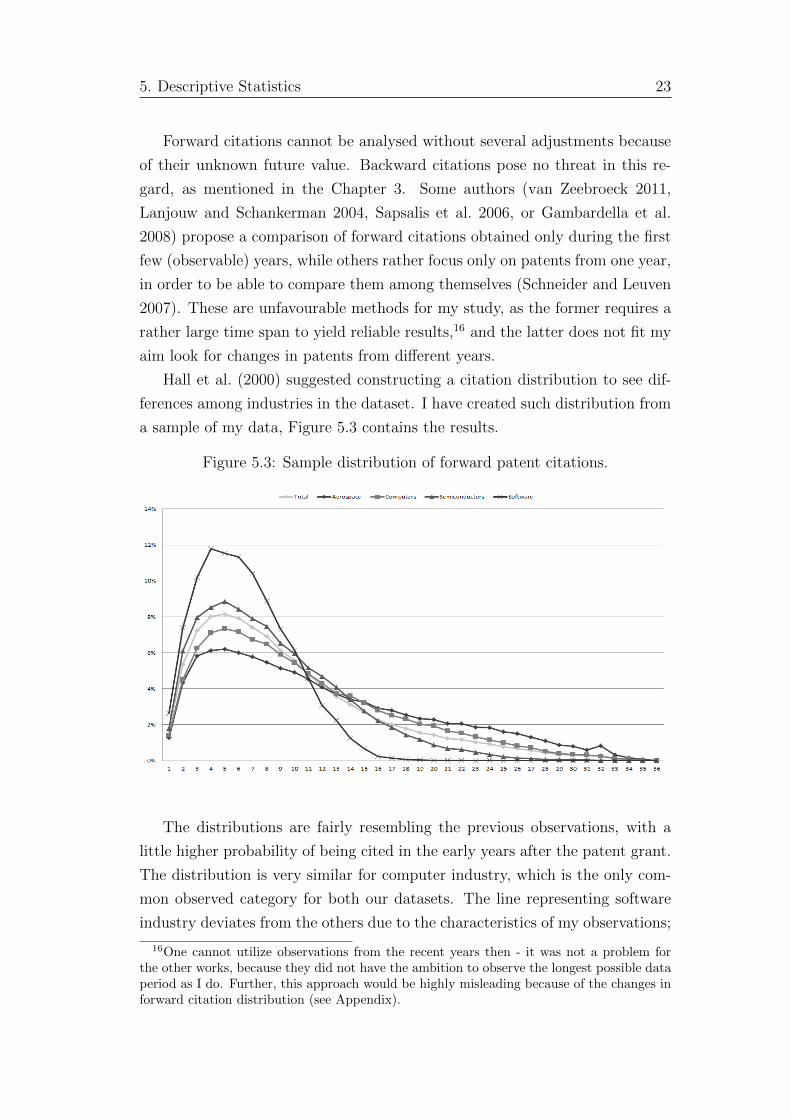
Hall et al. (2000) suggested constructing a citation distribution to see dif-
ferences among industries in the dataset. I have created such distribution from
a sample of my data, Figure 5.3 contains the results.
Figure 5.3: Sample distribution of forward patent citations.
The distributions are fairly resembling the previous observations, with a
little higher probability of being cited in the early years after the patent grant.
The distribution is very similar for computer industry, which is the only com-
mon observed category for both our datasets. The line representing software
industry deviates from the others due to the characteristics of my observations;
16One cannot utilize observations from the recent years then - it was not a problem forthe other works, because they did not have the ambition to observe the longest possible dataperiod as I do. Further, this approach would be highly misleading because of the changes inforward citation distribution (see Appendix).

5. Descriptive Statistics 24
the software companies in my dataset started to patent in the late 1980s, and
it is therefore impossible to observe patent citations for as long time period
as for the other technological fields, explaining the steeper decline and almost
zero probability of being cited past the age of 20.
The divergence for higher lags is again given by the fact that the companies
in software and semiconductor industry started applying for patent protection
later than those in aerospace and computer manufacturing industries. But
the variance in citation gains for early years is significant, and points at some
interesting facts, e.g. that the patents in aerospace industry seem to be relevant
for much longer period of time than the patents from semiconductor or software
industry (i.e. the same findings as in the case of backward citations). Such
differences were earlier suggested by Jaffe et al. (1993). They are expected
for the dissimilar nature of the industries; the rapid innovation in software and
semiconductor industry indicates lesser relevance of new inventions to the older
patents.
Hall et al. (2000) in his work further predicts the total number of forward
citations a patent would receive at a given age. Even though his method is
not usable in my study, he inspired me to develop my own approach. It is
fully described in the Appendix, I will only discuss the outcome here. First,
Table A.1 shows the number of forward citations obtained by patents from each
industry and time cohort up to 11 years after the patent grant in a sample from
my dataset (the numbers are weighted by the observed patents in each time
cohort, in order to be directly comparable). The data show a clear overall
increase in the number of forward citations obtained in the early years after
the patent grant. Patents granted between 2001 and 2005 are cited more than
two times as much as those granted between 1996 and 2000 in the first year,
and there is a sharp decline in the citations obtained in the latter years.
I have created sample cumulative distribution functions to be able to predict
the total number of forward citations a patent would obtain and to graphically
illustrate the change in the distribution (see Figure A.1). For newer patents,
the function is much steeper, meaning that the patents in these groups are pre-
dicted to obtain many more citations in the early years, but less in the latter.
That corresponds not only to the trend of rapid innovation (the distributions
of patents in semiconductor industry for the last two time cohorts are in fact
very different from the other industries, which would indeed refer to a sub-
stantial evolution in semiconductor industry during last 20 years), but also to
the suggested decline in patent value over time (and possibly the strategical

5. Descriptive Statistics 25
exploitation). Arguably, if a patent is obtained for strategical purposes, only
the patents applied for shortly after its grant (i.e. those entangled in the patent
thicket) ought to cite it, as the patent most likely does not bring any signifi-
cant technological improvement (the latter patents would not build upon the
invention).
The functions were then used to predict the total number of forward cita-
tions gained 31 after years the patent grant (i.e. the maximum observable years
for the earliest time cohort). The results are shown in Figure 5.2. We can see a
steady increase until 1996, followed by a steep decline until the end of the data.
Because the distribution of forward citations, just as the distribution of patent
value, is extremely skewed, the median may be more reliable for a conclusion.
Clearly, the trend is similar; however, the changes are much more gradual. It
is crucial to mention that the percentage of patents which have not obtained
a single forward citation has greatly increased. In fact, only about 2% of all
patents in my dataset issued in 1976 have not received a forward citation, in
comparison to 7 percent in 2002 and immense 20% in 2005. It seems that not
only the newer patents are cited less in general, but about one fifth of them
seems not to have any technological value at all.
To better understand the immense drop in forward citations, I have also
obtained the results for each industry. These are depicted in Figure 5.4.
Figure 5.4: Forward citations by industry.
Looking at it, it is clear that the previously mentioned trend varies heavily

5. Descriptive Statistics 26
across the industries. The patents of companies in aerospace industry (which
have shown to be more dependent on the prior inventions) seem to be very
stable over the observed period. It is in a high contrast with the other in-
dustries, particularly software industry. It seems that the patents in software
industry were of a very high technological value at first, but have lost their
value extremely as the time went by. That is perfectly logical, as the patents
from late 1990s (i.e. those applied for in the middle 1990s) laid the basics for
whole software industry,17 while the recent inventions are not so valuable and,
arguably, mainly strategical.18
To better understand patent citations as a whole, we must also look at
the numbers of patents in each industry (shown in Table C.2). There are less
patents observed in aerospace industry than in software industry, even though
software companies have started to patent much later. There are also more
patents in computer industry than in all the other industries together. From
these statistics and from the figures shown previously, I may conclude that
the number of backward citations (i.e. the number of inventions that a given
patent is built on) is rather similar for all the industries. On the other hand,
the number of forward citations (i.e. the technological value of a given patent)
varies heavily because the industries vary as well. It is not surprising that
the number of forward citations gas grown for most of the observed period in
computer industry simply because not only the total amount of issued patents
grew each year, but also because the growth rate of newly issued patents was
positive each year (i.e. there were more patent grants each year). To better
illustrate this, I use the same methodology as in the case of backward citations,
to weight forward citations as well. Figure C.4 exhibits the results.
We can see that the steady increase within computer industry is now just
rather flat, with only one permanent increase between 1986 and 1989. Yet one
must keep in mind that there is no strong theory suggesting the forward patent
citation counts would be biased by the increasing number of patents, however
likely it might be; thereby, I rather restrain myself from making conclusions
regarding the issue.
Software development company Oracle has the most valuable patents re-
17That applies for the patents granted prior to 1990 as well, but those are not shown inthe Figure 5.4 for their low counts, which could have biased the results.
18Indeed, some famous recent patent applications include specific movement of icons onthe screen by Apple, ”upgrade” button for applications by Lodsy, or one-click purchase byAmazon. (Sakmann 2012)

5. Descriptive Statistics 27
garding forward citations with an average of 34.2, while its competitor, Red
Hat, only has 4.6 forward citations per its patent on average.19
5.2 Family Size
Unlike citations, family size as a variable does not need to be adjusted. EPO
searches other patent offices’ patents by their priority numbers20 and puts to-
gether similar patents from all around the world. These not only include the
exactly same invention, applied for in different countries, but also all similar
inventions, based on one priority number.21
Figure 5.5: Family size, based on date of application.
Figure 5.5 shows the evolution of the average family size within my dataset.
19The data are the averages for all patents for a given company and a given year.20A priority number is assigned for each new invention, and thus identifies the priority
claim of its owner. Priority claim may be used by a patent application to claim priority fromanother previously filled application, in order to take advantage of the filling date of theformer one. In other words, it is enough to apply for a patent in one country and then applyfor the same patent later (although within one year from the first application) in anothercountry, while taking benefits of having applied for it in the first country before. Any otherinventor who would apply for the same patent between both applications would not gain theright for his invention, even though he would be first in the national regard. This applies toall countries which are party to the Paris Convention. Such behaviour is desirable by firms,delaying their expenses for applications in other countries up to a year without a menace oftheir competitors applying first.
21One invention may have more than one priority number. EPO describes patent familyas: “All the documents directly or indirectly linked via a priority document belong to onepatent family.” (http://www.epo.org/searching/essentials/patent-families/inpadoc.html)

5. Descriptive Statistics 28
There is a rather steep decline until 1984, followed by a further steady down-
ward trend over the years. The evolution in the first observed years and its
sudden change interestingly corresponds to the increase in patent applications
after the establishment of the Court of Appeals. It may be so that those who
applied for patents before the establishment also sought patent protection in
more countries. Assuming family size to be truly a correlate of patent value,22 I
may conclude that patents are now much less valuable than they were before. I
have again obtained the results for each industry separately as well (see Figure
C.6). But unlike citations, family size shows no important differences across
the industries.
5.3 Renewals
Patents in the present US patent system must be renewed at the end of a certain
period of time to remain valid. This only applies to utility patents, whereas
design and plant patents cannot be renewed (those are granted for much longer
though). Currently, every patent is valid for 4 years after the filling date, and
must be paid for in the last 6 months of its validity in order to be renewed (with
a possible slight delay, which is then fined). Payment validates the patent for
another 4 years, up to 8 years from the grant date. The same procedure may be
repeated twice more, the last payment extends patent’s life up to 20 years from
the application date. The fees are substantially higher for further renewals, and
are currently at $1,130, $2,850, and $4,730 for patents due at 3.5, 7.5, and 11.5
years, respectively.23 These apply only to large firms, smaller firms’ payments
are exactly half of these. None of the companies in my dataset is considered
small in this regard. Only patents with the application date after December
12, 1980, are subject to maintenance fees; thus, it makes no sense to include
any earlier issued patents in my analysis. Beside that, I must only consider
data with the date of the grant up to and including year 2007, i.e. older than
4 years, to be able to observe patent renewal decisions.
Statistics of renewals are fairly interesting. More than 90% of patents in my
dataset were renewed at least once. This is similar for all the observed years,
22The meaning of family size is a little bit different in this case from what was mentionedin Chapter 3. The outcome remains the same though - larger family size should point atmore valuable patents both because it has been applied for in other countries and becausethere are more inventions build upon the underlying idea (i.e. the same reasoning as om thecase of forward patent citations.)
23http://www.uspto.gov/web/offices/ac/qa/ope/fee092611.htm

5. Descriptive Statistics 29
with an exception of years 1987 to 1991. Computer manufacturing industry has
much lower values in the recent years, falling down to 75% in 2004, whereas
the other three industries exhibit consistent figures above 90%. We can see
that it is very common to extend patent validity at least once. The numbers
may be higher due to the size of observed firms though. The first maintenance
fee may be rather insignificant for companies with yearly revenues exceeding
billion dollars. Only the most useless patents would not be renewed at least
once.
Figure 5.6: Renewal data, patents granted from 1976 to 1999.
To make things more interesting, I have divided my dataset, limited by the
specifications of the renewal system, into three categories: from the application
date after December 12, 1980, to the grant date up to and including 1999; with
the date of the grant between 2000 and 2003; and finally, with the date of the
grant between 2004 and 2007 (i.e. patents, which could have been renewed
three times, two times, and once, respectively). It is then possible to compare
patents that could have been extended for the same period of time. Figure
5.6 exhibits how volatile actually renewal statistics are. On average, about the
same number of patents were renewed once and twice (and could have been
renewed three times), and over 40% of patents were renewed for the full term
in the first category. There was a major decline in full renewals, followed by
low values between 1984 and 1991, while the number of patents not renewed
at all increased. Remarkably, there was an increase in once renewed patents,

5. Descriptive Statistics 30
at the same time. For the patents with the date of the grant after 1991, the
probability of being renewed for whole 20 years increased up to 80%, with a
slight decline from 1997 to 1999.
The second category (patents granted between 2000 and 2003) is summa-
rized in Figure C.2. It shows a similar trend regarding the number of patents
renewed once or not at all as Figure 5.6. The percentage of patents renewed
twice (i.e. for the longest possible period) is above 70%. This again follows
the decision-making from the first category, looking at patents renewed at least
twice. Patents with the date of the grant between 2004 and 2007 are shown in
Figure C.3. About 90% of all patents were renewed. The number is a little bit
lower than in the previous years due to the decline in the renewals in computer
manufacturing industry. That said, I may again conclude that the overall value
of patents (assuming that renewal data are indeed correlated with it) had been
rather stable over time, but dropped significantly in the last observed period
in computer manufacturing industry.
5.4 Patent Trades
Following the discussion from Serrano (2005), patents are traded because some
companies are more productive in use of a given patent. The cost of such trans-
action, accounting for the cost of implementation, is the reason for selection of
such patents, i.e. only the more valuable patents should be traded. According
to his results, the probability of a patent being traded decreases from the date
of the grant, with a slight increase just after being renewed. That said, my
dataset, curtailed due to the limitations of the other variables I use, should
provide reliable data even for the recently issued patents.
Arguably, the assumed strategical behaviour of companies regarding their
patent portfolios in recent years may have devalued patent trade data as a cor-
relate with patent value, due to a higher probability of trading whole portfolios
for strategical reasons, rather than to obtain highly valuable patents. Because
I only use patent trades in my analysis up to year 2005 and Figure 5.7 shows
no noticeable changes until then, at least in the trade volumes, I made an as-
sumption that if patent trade data have indeed lost their explanatory power,
then only in the very recent years and my analysis should thus not be affected.
Figure 5.7 demonstrates patent trade statistics.24. There is a very significant
24The USPTO database contains general data about patent ownership and its changes. Itwas possible not only to see that a patent has changed its owner, but also for what reason

5. Descriptive Statistics 31
rise and fall between years 1981 and 1984. The explanation for such activity
would be very hard and doubtful, and thus I refrain from it. Of higher interest
is the steady increase followed by a decrease, from 1986 to 1994 and 1995 to
2006, respectively. The results follow the other patent value correlates (e.g.
forward patent citations).
Figure 5.7: The average number of traded patents.
I have once more obtained the results separately for each industry, those are
depicted in Figure C.7. We can see a rather striking difference in the trade of
computer patents in 1990s, but it seems that it was only a temporary deviation,
followed by a steep decrease.
5.5 The Other Variables
To support the indicators correlated with patent value, several other variables
were obtained. Those are pure patent characteristics, which do not rely on
further management of the patent or time passed since the date of the patent
issue; they are all known by the time of the patent grant and do not evolve any
further.
These complexity measures include: the number of inventors per patent ap-
plication, the number of different International, European and US patent clas-
(i.e. direct trades, acquisitions, court decisions etc.) The data I present in this paper containonly the direct patent trades and licence agreements, which should indicate a higher patentvalue in a similar way to patent trades.

5. Descriptive Statistics 32
sification, and backward citations to other patents. Figure 5.8 shows changes
in those indicators.
Figure 5.8: The other patent variables.
Clearly, the average number of inventors has grown over the recent decades.
It may indicate a lesser capability of firms to invent, although the companies
in my dataset are very large and it is possible that they simply spend more re-
sources on research, while employing more scientists. Patents of semiconductor
company Applied Materials have the highest average number of inventors per
patent (3.5), whereas software company Red Hat only 1.1.
US and European patent classifications show no significant development
throughout the observed period of time. International classification, on the
other hand, shows a constant decrease, with a very significant drop in 2006.
This is due to several changes in its measurement.25 The last change was on
January 1st, 2006. Detailed statistics of all obtained variables are shown in
Table C.3.
25http://pesquisa.inpi.gov.br/ipc/guide/en/guide.pdf

Chapter 6
Empirical analysis
In this section, I further utilize my dataset to perform an empirical analysis. In
the first part, several econometric models are employed to discover the relation-
ships among my variables; to show the differences in my results, compared to
the previous literature; to provide additional information regarding the effec-
tiveness of the variables (as shown in Table 3.1); and finally, to discover whether
the explanatory variables are sufficient to explain the year-to-year differences
in the value correlates. Then, I use DEA to measure relative efficiency with
which the observed companies transform certain inputs into patents, in order
to further expound my observations and to provide some empirical evidence
for the theory of strategical patents.
6.1 Econometric analysis
The econometric approach has been developed by e.g. Lanjouw and Schanker-
man (2001), Gambardella et al. (2008), or Schneider and Leuven (2007). I
estimate 4 different models which more or less arise from their work, and dis-
cuss the differences in my results compared to what has been found before.
The first two models explain how much of the variance in patent value is ex-
plained by the indicators contained in the patent document, an approach used
by Bessen (2008). In these models, patent value is substituted by its correlates
(forward citations and family size), which have previously been shown to have
a very strong and significant relationship with it (see Table 3.1), because the
value itself cannot be observed. Due to the nature of forward citations, the
number of observations in the first model is lower than in the model using fam-
ily size as the dependent variable, as I had to restrict the dataset from the right

6. Empirical analysis 34
to work with reliable data. The citation values are the predicted forward cita-
tion counts a patent would obtain 31 years after the grant. At the same time,
I check the importance of time and industrial affiliation through the dummy
variables.
The latter two models build upon the works of Reitzig (2003a), or Lanjouw
and Schankerman (2001), and elucidate the importance of patent characteristics
for the managerial decisions, such as whether to renew or to trade a patent.
This is essentially different from the former two models; the question here is
no longer if a certain characteristic is connected to patent value, but how can
it affect the decision tree of patent’s life. Therefore, I also include forward
citations as an explanatory variable in the regressions, to see the significance
of patent’s “performance” on it’s validity and the probability of a change of
the owner. Again, I put all the time and industry dummies in the regression.
Furthermore, I estimate all four models twice more; once with a linear and once
with a quadratic time trend, to test whether the other explanatory variables
(backward citations, the number of inventors and priority numbers, patent
classifications, and the industrial dummy variables) are sufficient to explain
the differences in patent value.
Following Sapsalis et al. (2006), I use the negative binomial model to esti-
mate the equations with forward citations (Fcit) and patent family size (Fsize)
as the dependent variables for their skewed nature (see Table C.3 for the de-
tailed statistics). The individual units yi follow a Poisson regression model
(with parameter λi), with an omitted variable ui, such that exp(ui) follows a
gamma distribution with mean 1 and variance α:
yi ∼ Poisson(µ∗i )
µ∗i = exp(xiβi + ui)
exp(xiβi + ui) ∼ Gamma(1
α,
1
α)
where βi is the vector of parameters, xi is the vector of explanatory variables,
and α is the overdispersion parameter. The vector of explanatory variables con-
sists of the number of inventors per patent application (inventors), the number
of different International (INTclass), European (EUclass) and US (USclass)
patent classification, and backward citations to other patents (Bcit). Most of
the variables are in logarithmic form for easier explanation of the outcome.
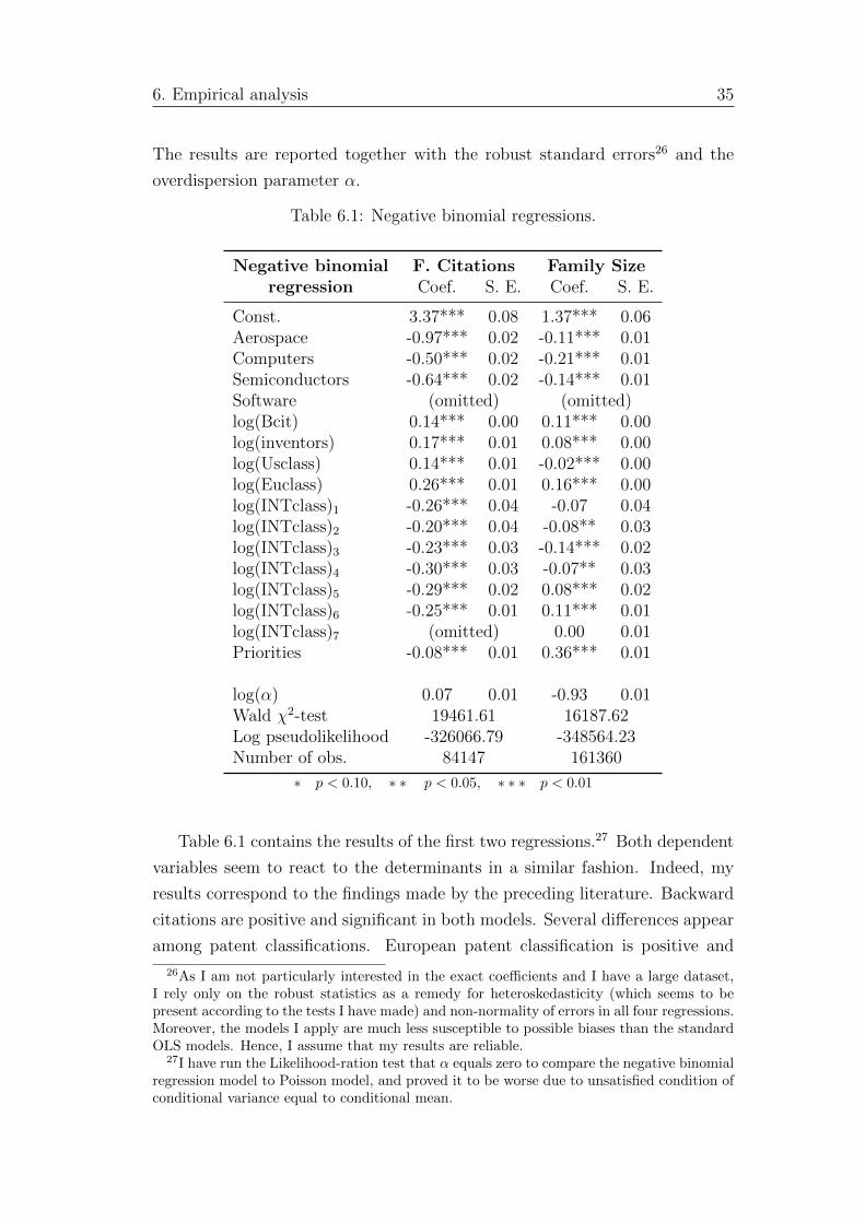
6. Empirical analysis 35
The results are reported together with the robust standard errors26 and the
overdispersion parameter α.
Table 6.1: Negative binomial regressions.
Negative binomial F. Citations Family Sizeregression Coef. S. E. Coef. S. E.
Const. 3.37*** 0.08 1.37*** 0.06Aerospace -0.97*** 0.02 -0.11*** 0.01Computers -0.50*** 0.02 -0.21*** 0.01Semiconductors -0.64*** 0.02 -0.14*** 0.01Software (omitted) (omitted)log(Bcit) 0.14*** 0.00 0.11*** 0.00log(inventors) 0.17*** 0.01 0.08*** 0.00log(Usclass) 0.14*** 0.01 -0.02*** 0.00log(Euclass) 0.26*** 0.01 0.16*** 0.00log(INTclass)1 -0.26*** 0.04 -0.07 0.04log(INTclass)2 -0.20*** 0.04 -0.08** 0.03log(INTclass)3 -0.23*** 0.03 -0.14*** 0.02log(INTclass)4 -0.30*** 0.03 -0.07** 0.03log(INTclass)5 -0.29*** 0.02 0.08*** 0.02log(INTclass)6 -0.25*** 0.01 0.11*** 0.01log(INTclass)7 (omitted) 0.00 0.01Priorities -0.08*** 0.01 0.36*** 0.01
log(α) 0.07 0.01 -0.93 0.01Wald χ2-test 19461.61 16187.62Log pseudolikelihood -326066.79 -348564.23Number of obs. 84147 161360
∗ p < 0.10, ∗ ∗ p < 0.05, ∗ ∗ ∗ p < 0.01
Table 6.1 contains the results of the first two regressions.27 Both dependent
variables seem to react to the determinants in a similar fashion. Indeed, my
results correspond to the findings made by the preceding literature. Backward
citations are positive and significant in both models. Several differences appear
among patent classifications. European patent classification is positive and
26As I am not particularly interested in the exact coefficients and I have a large dataset,I rely only on the robust statistics as a remedy for heteroskedasticity (which seems to bepresent according to the tests I have made) and non-normality of errors in all four regressions.Moreover, the models I apply are much less susceptible to possible biases than the standardOLS models. Hence, I assume that my results are reliable.
27I have run the Likelihood-ration test that α equals zero to compare the negative binomialregression model to Poisson model, and proved it to be worse due to unsatisfied condition ofconditional variance equal to conditional mean.
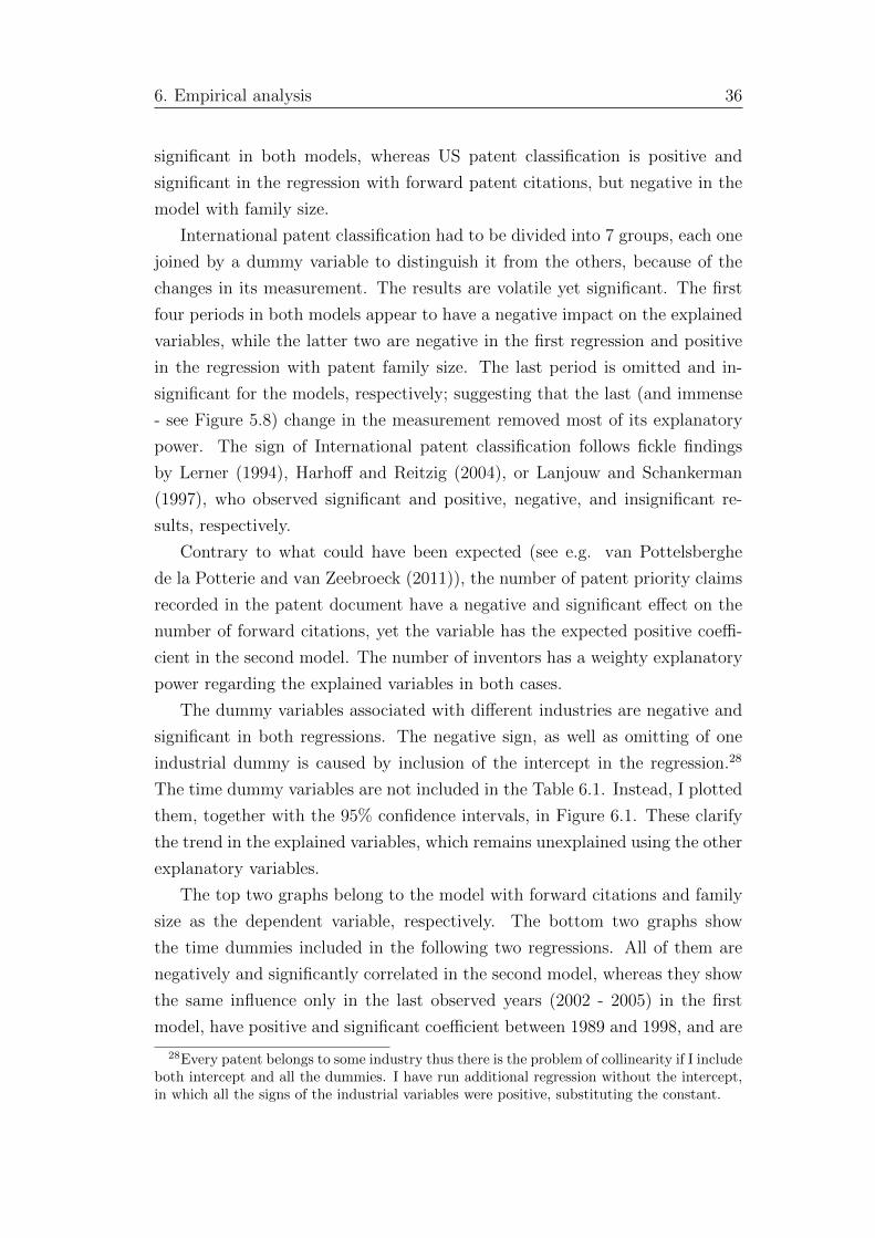
6. Empirical analysis 36
significant in both models, whereas US patent classification is positive and
significant in the regression with forward patent citations, but negative in the
model with family size.
International patent classification had to be divided into 7 groups, each one
joined by a dummy variable to distinguish it from the others, because of the
changes in its measurement. The results are volatile yet significant. The first
four periods in both models appear to have a negative impact on the explained
variables, while the latter two are negative in the first regression and positive
in the regression with patent family size. The last period is omitted and in-
significant for the models, respectively; suggesting that the last (and immense
- see Figure 5.8) change in the measurement removed most of its explanatory
power. The sign of International patent classification follows fickle findings
by Lerner (1994), Harhoff and Reitzig (2004), or Lanjouw and Schankerman
(1997), who observed significant and positive, negative, and insignificant re-
sults, respectively.
Contrary to what could have been expected (see e.g. van Pottelsberghe
de la Potterie and van Zeebroeck (2011)), the number of patent priority claims
recorded in the patent document have a negative and significant effect on the
number of forward citations, yet the variable has the expected positive coeffi-
cient in the second model. The number of inventors has a weighty explanatory
power regarding the explained variables in both cases.
The dummy variables associated with different industries are negative and
significant in both regressions. The negative sign, as well as omitting of one
industrial dummy is caused by inclusion of the intercept in the regression.28
The time dummy variables are not included in the Table 6.1. Instead, I plotted
them, together with the 95% confidence intervals, in Figure 6.1. These clarify
the trend in the explained variables, which remains unexplained using the other
explanatory variables.
The top two graphs belong to the model with forward citations and family
size as the dependent variable, respectively. The bottom two graphs show
the time dummies included in the following two regressions. All of them are
negatively and significantly correlated in the second model, whereas they show
the same influence only in the last observed years (2002 - 2005) in the first
model, have positive and significant coefficient between 1989 and 1998, and are
28Every patent belongs to some industry thus there is the problem of collinearity if I includeboth intercept and all the dummies. I have run additional regression without the intercept,in which all the signs of the industrial variables were positive, substituting the constant.
6. Empirical analysis 37
Figure 6.1: Coefficients and 95% confidence intervals of time dum-mies, all four regressions. Top two are the negative bino-mial regressions (with Fcit and Fsize as the dependentvariables, respectively), bottom two are the probit regres-sions (with renewals and trades, respectively).
insignificant otherwise. This behaviour is directly connected to the evolution
of forward citations as shown in Figure 5.2. Both linear and quadratic time
trends are significant with negative sign in both regressions.
The overall results correspond to the prior findings regarding the sign and
the significance of backward citations, and US and International classifications.
At the same time, on the other hand, suggest that European patent classifica-
tion has a positive and significant explanatory power regarding patent value,
while priorities seem ambiguous.
The latter two models use patent renewal decisions and patent trades as the
dependent variables. Because patent renewals can be fully observed for only a
limited period of time within my dataset, I rather employ a model estimating
the probability a patent would be renewed at least once. The other model
estimates probability that a patent would be traded, building upon findings
made by Serrano (2005). Fforward patent citations are used in their percentile
form.29 Unfortunately, the low number of observations for certain time peri-
29The percentile values are computed for each year and each industry separately. Thepercentile form is used for two reasons: first, it completely standardizes the values of forwardcitations, which have to be predicted otherwise. This was not possible in the previous twomodels due to citations being used as the correlate of patent value, which must be allowed to

6. Empirical analysis 38
ods and industries limit the data for software and aerospace industry in the
percentile estimation.
Table 6.2: Probit regressions.
Probit Renewal Tradedregression Coef. S. E. Coef. S. E.
Const. 3.54*** 0.32 -2.22*** 0.13Aerospace -1.62*** 0.11 0.63*** 0.04Computers -1.61*** 0.10 0.73*** 0.03Semiconductors -1.32*** 0.11 0.41*** 0.03Software (omitted) (omitted)
Fcit(percentiles) 0.42*** 0.02 0.04* 0.02log(Bcit) -0.01 0.01 -0.03** 0.01log(inventors) -0.02* 0.01 -0.07*** 0.01log(Usclass) -0.07*** 0.01 -0.03** 0.01log(Euclass) 0.10*** 0.01 -0.04** 0.01log(INTclass)1 (omitted) 0.15* 0.07log(INTclass)2 0.00 0.16 0.01 0.06log(INTclass)3 -0.07 0.08 0.15** 0.06log(INTclass)4 -0.23*** 0.05 0.02 0.04log(INTclass)5 -0.06 0.04 0.20*** 0.03log(INTclass)6 0.05** 0.02 0.17*** 0.02Priorities 0.03* 0.01 -0.02** 0.01
Wald χ2-test 2238.86 1960.54Log pseudolikelihood -21021.62 -33389.71Number of obs. 79029 84147
∗ p < 0.10, ∗ ∗ p < 0.05, ∗ ∗ ∗ p < 0.01
The results are shown in Table 6.2. The constant and the coefficients of
the industrial dummy variables act differently in both models. This is not
unexpected if we look at the descriptive statistics of renewal data and patent
trades; over 90% of all patents were renewed at least once, but only about 13%
of all patents were traded. The most important result of the regression with
patent renewal data is definitely the significance and the positive sign of forward
evolve over time. Second, the latter two models help to answer the question ”Why was thispatent renewed (traded) and the others were not?” The percentile values directly comparethe given patent to all patents granted in the same year and industry, which substitutes thecomparison that the management would have at the time of the decision. I do not includefamily size variable in the regression, as its value also depends only on the decision of themanagement.

6. Empirical analysis 39
patent citations. It seems that the decision whether to extend patent’s validity
does indeed depend on the value of the patent. The second model exhibits
results very similar to findings of Serrano (2005). Valuable patents, measured
by forward patent citations, are truly more likely to be traded. Together with
the previous outcomes, I may conclude that International classification has lost
nearly all its explanatory power. Further, my dataset yields similar results as
those in the previous literature, and the managerial decisions depend on the
value of the patent, as expected.
The time dummies are mostly insignificant for the former model with re-
newal data, only years from 1999 on seem to be statistically significant at the
5% level. The opposite is true in the case of the latter model. Most of the year
dummies are significant and positively correlated (whereas they are negatively
correlated in the first model), suggesting that patent trades were more ”fash-
ionable” in certain years, but renewal decisions remained constant. However,
the estimations with the time trends included show quite the opposite; both are
significant in the first model, and insignificant in the second. The explanation
is present in the plots of the time dummies in Figure 6.1. First model shows
a downward trend in the time dummy coefficients, while there are significant
ups and downs in the other.
The test statistics for the overall significance of the models show no doubt
that all four models are much better than their alternatives with no predictors
(i.e. the hypothesis H0 = β1 = ... = βn = 0 can be rejected even at 0.1%
significance level). Additional statistics to compare models are shown in Tables
C.4 and C.5.
6.2 DEA analysis
If the theory about the strategical use of patents, suggested by e.g. Macdonald
(2004), is indeed correct, there should be some visible changes in the company’s
performance regarding their patent portfolios. Essentially, a company behaving
strategically is supposed to be less efficient in creating technologically valuable
patents, and more efficient in producing high number of patents in general at
the same time. Such company does not rely on valuable inventions to secure
itself a market advantage, it endeavours to create large patent thickets around
key patents of the competition instead. And to create such thickets, it requires
a large number of patents, whatever quality they may be.
To search for these changes, I use Data Envelopment Analysis (DEA), a

6. Empirical analysis 40
method introduced by Farrell (1957) and further developed by Charnes et al.
(1978), which has been extensively applied to evaluate performance in manu-
facturing and service operations. DEA measures relative efficiency of a homo-
geneous set of decision making units (DMU) through calculating an efficiency
frontier and then comparing each DMU to it. DEA allows multiple inputs
and outputs in natural units to be used at the same time. The final relative
efficiency score is then computed as:
Efficiency = Weighted Sum of OutputsWeighted Sum of Inputs
Essentially, DEA only requires inputs and outputs to be given, not the produc-
tion function (i.e. the ”black box”).
Further, DEA allows for both constant and variable returns to scale, which
is useful for my work, as the companies in my dataset are of dissimilar sizes
and, more importantly, have different propensity to patent; thus, they perform
research and development with a distinct effort. Constant returns to scale
assume that the maximal effectiveness remains the same for production at a
small scale as at a large scale. In other words, a company producing 10 units of
output from 10 units of input is supposed to produce 100 units of output from
100 units of input, if it remains fully effective at both times. Variable returns
to scale assume that a company may be fully effective at both small and large
scale, even though the input-output ratio is different.
Needless to say, the results are very different, depending on which method
is used. There are many reasons why it would be reasonable to assume either of
them. Arguably, it should cost the same amount of money and time to create
an invention of a certain technological value, no matter whether the inventors
work for a small or a large company. Moreover, the average number of inventors
per patent is very similar for all companies in my dataset, even though they
are of considerably different sizes. On the other hand, it is rational to expect
that a large company may be better in R&D in general; that the marginal
product of additional employee in R&D may be increasing; that larger patent
portfolio may mean lesser administrative costs per patent on average; or that
larger companies have more productive employees, and thus the returns to scale
should be variable.
Another problem is the rather small number of observed DMUs for my
analysis. In order to obtain precise estimates of efficiency under the variable
returns to scale assumption, there would have to be enough DMUs of similar

6. Empirical analysis 41
sizes. Unfortunately, this is not the case of my dataset, so the final results may
be a little different compared to use of a larger dataset.
Bound et al. (1982) or Griliches (1981) have shown that the elasticity of
patenting with respect to R&D employment is close to unity; therefore, I may
assume that the constant returns to scale can be used in this situation. Nev-
ertheless, these works are rather old and the situation may have changed dra-
matically since then. Because the question remains unanswered, I have decided
to include both models in my analysis. Furthermore, as the data are in the
logarithmic form to obtain reliable results (i.e. to prevent outliers from ruining
the analysis), the differences in the size of the companies are no longer so clear.
Consequently, both methods ought to yield similar results.
Following Talluri (2000), assuming that there are n observed DMUs, each
with m inputs and s outputs, the relative efficiency is computed as:
max
k=1∑s
vkykp
j=1∑m
ujyjp
s.t.
k=1∑s
vkyki
j=1∑m
ujyji
≤ 1, ∀i
vk, uj,≥ 0, ∀k, j,
where k=1,...,s, j =1,...,m, i=1,...,n, yki = amount of output k produced by
DMU i, xji = amount of input j processed by DMU i, vk = weight given to
output k, and uj = weight given to input j. This fractional problem may then
further be transformed into linear program:
maxk=1∑s
vkykp
s.t.
j=1∑m
ujyjp = 1
k=1∑s
vkyki −j=1∑m
ujxji ≤ 0, ∀i
vk, uj,≥ 0, ∀k, j.

6. Empirical analysis 42
Relative efficiency score means that there is always at least one fully efficient
DMU in the sample, however it does not tell us anything about the overall
efficiency. Yet it is sufficient for my analysis, as I am only interested in the
changes throughout the observed time period. As said above, the efficiency
depends heavily on the assumptions. There are usually more fully efficient units
under variable returns to scale than under constant returns to scale assumption,
because the efficiency frontier is then non-linear.
DEA has also several disadvantages, as mentioned in Prochazkova (2010).
First of all, the number of observations is suggested to be at least three times
higher than the number of input and output variables together. Because of a
limited number of observations in my data sample,30 I must have been very
careful not to use an extensive amount of variables in the analysis. The second
problem is connected to the efficiency. The efficiency frontier may be mislead-
ing if there are outliers present in the dataset. To prevent this, I have run two
outlier detection analyses under MedCalc program with logarithmic transfor-
mation of my data to see possible outliers both from the left and the right side.
Neither of the tests showed possible outliers at the 5% Alpha-level, my data
seem to be useful for the analysis then.
Because I am mainly interested in patents as the company’s output, inputs
connected with patents must have been chosen. Again, since I required a
variable common and obtainable for all the companies in my dataset, there were
not many options. I have obtained the data about the number of employees
(unfortunately, whole company’s workforce, not only the employees in R&D,
because such data were scarce), research and development expenses, and the
net profits the company had in a given year. Because net profits may be
negative and thus pose a threat to the analysis, I have then decided to only
use the former two variables as my input (the data were then adjusted for the
inflation). I have transformed both of them into natural logarithms because of
the large differences among the companies.
Following the preceding discussion, I use the number of patents the company
30The financial data of observed firms are publicly available because the companies arelisted on the stock exchange, but the necessity to publish the reports on-line was first es-tablished in 1994. Despite searching in various databases and writing to the companies forearlier reports, I have obtained just a few of these. As it is necessary for the analysis tohave a sufficient number of observations from the same year, the data are limited by 1994from the left. At the same time, the patent data are based on the date of the application (asthe opposite to the date of the grant in the previous sections), the time difference betweenpatent application and patent grant, and the use of forward citations as the DEA output; Ihave limited the dataset by 2003 from the right.

6. Empirical analysis 43
has applied for in a given year (but only those which were later granted) and
the average of composite rating of such patents as the output variables. Again,
the number of patents have been transformed into natural logarithms. The
composite rating consists of patent characteristics shown to be heavily and
positively correlated with patent value. These are forward citations, family
size, renewal data and patent trades.31 Because the former two are dispersed
count variables, whereas the latter two are binary, I have transformed the first
two into natural logarithms for the final rating to similarly depend on all four
variables.32 It is then computed as:
Rating = ln(1 + Fcit) + ln(1 + Fsize) +Renewed+ Traded
DEA analysis also allows to set restrictions on the computed weights (e.g.
that the weight of research and development expenditures cannot be more
than twice as high as the weight of the number of employees). I tried many
different restrictions; however, none of them meant a significant difference in the
results. In the end, the final models are used without any weight restrictions. I
estimated 6 different models to be able to see the changes from as many points
of view as possible. The models differ in the outcome variables used - one model
only with the raw number of patents (transformed into logarithm form), one
only with the composite rating, and one model using both outcome variables.
Every model was then estimated both assuming constant and variable returns
to scale.
As I am mainly interested in the changes of efficiency for a given company
across the time, simple cross-sectional analysis is not sufficient. Panel data are
better than cross-sectional in this sense because one can then not only compare
one company to another, but is also able to see the change over time.
The downside of panel data usage is a possible bias caused by the unob-
servable technological improvement, especially if the data period is long. The
DMU from the beginning of the dataset is then compared to the same DMU
at the end of the dataset, which may operate under completely different cir-
31While all of these variables are correlated with patent value, they are almost uncorrelatedamong themselves (see Table C.6 in the Appendix), meaning that each of them explains adifferent part of patent value. Therefore, it is favourable to include them all in the analysis.
32Keep in mind that the exact outcome is not important, as I am not interested in thenumber, but only in its change over the observed period. The previous literature suggests thatforward citations are the most reliable correlate with the patent value, thus the compositerating still relies on forward citations the most. The descriptive statistics are shown in theTable C.7.
6. Empirical analysis 44
cumstances. For that reason, rather than using simple panel data estimation
method, I employ DEA Window Analysis, a method developed by Charnes
et al. (1985), which enables me to only compare each DMU with the others
within a given time period. As explained in Chung et al. (2008), assume that
there are l = 1, ..., N companies in the dataset, each observed for all 1, ...,M
years.33 The window length (the number of years within which all the DMUs
are compared) is given by K. I follow Charnes et al. (1985) and set K = 3 as
it seems to yield the most accurate results. The first window is then composed
of all the DMUs from years 1, 2, and 3 (1994, 1995, and 1996, respectively),
the second from years 2, 3, and 4, and so on; generally years j = i,...,i+K-1,
where i = 1,...,M-K+1.
The estimation is separate for each window, each DMU in the window is
then characterized by its efficiency Elij. These are reported in the Table C.8.
Further, to be able to compare the company among the others, the average
efficiency is computed as:
Ml =
M−K+1∑i=1
i+K−1∑j=i
Elij
K × (M −K + 1), l = 1...N
Table C.7 shows descriptive statistics of the variables used. Each observed
year of company’s performance is treated as an unique DMU. Because the
detailed results are extensive, I only include a sample results from software
industry (both outcome variables included) in Table C.8. Each company is
observed over 10 years, each row exhibits one window of the DEA analysis.
Bold are the average efficiency scores for a given year. We can see that there
is a clear downward trend in the case of Adobe, which seems to worsen its
performance in patent production. Microsoft, on the other hand, seems rather
stable over time. The results are pleasingly similar across different windows,
suggesting that the results are precise.
The summary results of the DEA analysis are shown in Tables C.9-11.
We can see that the assumption of variable returns to scale produces higher
estimates than constant returns to scale. The efficiency varies significantly
among the companies and the observed years; however, the numbers are very
similar for companies within an industry.
33I am not able to utilize my full dataset using this method, as several companies areobserved for less than 10 years because they went public at a later date. The analysis thenonly uses 13 out of total 25 companies.
6. Empirical analysis 45
Companies in semiconductor industry seem to be highly effective in general,
but the efficiency is lower when only the composite rating is used as the outcome
variable. This is similar to all industries and suggests that the companies are
more efficient in producing patents, than in producing valuable patents. Altera
is the most efficient company overall, whereas Boeing or the other companies
from aerospace industry seem not to be performing well at all. Interestingly,
IBM, which has publicly announced that it is more profitable for it to create
patent thickets than to make valuable inventions (Bessen 2004), is indeed just
poorly efficient in the model with only the composite rating as the outcome
variable, but it is rather peerless in creating patents in general.
All companies apart from Dell and United Technologies had improved their
efficiency in creating patents with given inputs over the observed period. The
results of the third model (composite index as the outcome variable) are not
so clear. The overall trend is negative under the assumption of constant re-
turns to scale, yet it is rather constant or positive assuming variable returns to
scale. Unlike in the models with raw patent numbers and both outcome vari-
ables (where the results were similar under both assumptions), it seems that
the model with composite rating shows certain deviations. It is not surprising
though; continuing the discussion in the beginning of this section, the results of
the model with pure patent counts as the outcome variable (and therefore also
the results of the model with both outcome variables) allow both the inputs
and the outputs to increase with the size of the company. Nevertheless, the
composite rating depends more on the propensity to create valuable inventions,
rather than on the size of the firm. Thereby, the models with both outcome
variables and raw patent numbers as the outcome variable exhibit similar re-
sults under both assumptions, because it seems that it indeed takes the same
amount of work and money to develop a new invention for both a small and a
large company. But constant returns to scale seem not to be favourable in the
model with the composite rating as the outcome variable - it is definitely not
true that a company with ten times higher input volume is supposed to create
inventions of ten times higher technological value.
That said, I may conclude that the overall trend in the efficiency regarding
transformation of inputs into valuable outputs (based on the estimates under
variable returns to scale assumption) is increasing. Although, one must keep in
mind that those results may be biased a little bit due to rather small dataset.
Yet it is not united for all companies within an industry. Perhaps the efficiency
depends more on the individual behaviour and the decision making of the

6. Empirical analysis 46
firm, than on the industry itself. Indeed, the fact that the companies became
more efficient in creation of patents in general, and diverged in the efficiency of
creating valuable patents, suggest that the trend of relying heavily on patents is
similar to all industries. However, the decision whether to aim for the valuable
patents at the same time was rather individual. Adobe, for example, had
doubled its efficiency in creating patents, but, its efficiency in making valuable
patents had decreased at the same time.
Summarized, the results are following: there is indeed a visible and a rather
strong increase in the efficiency of transformation of the research and devel-
opment inputs into patents in general. The trend is unclear in the case of
transformation of inputs into valuable patents, and seems to depend heavily on
the decision making within the company. According to the literature on strate-
gical patents, the higher efficiency in creating patents in general was expected.
The efficiency of creating valuable inventions, however, ought to be decreas-
ing, as companies spend more resources on creating less valuable inventions,
because the technological value of their patents does not need to be high. The
results point out that not all the companies in my dataset have decided to aim
for patent portfolios of a lesser technological value, or at least some of them
seem to produce valuable inventions more efficiently than before.
Chapter 7
Conclusion
Patents represent a substantial institution in today’s world, providing a pos-
sibility to possess and treat an intangible asset as if it were a material thing.
Importantly, the ownership is then under the law protection and the patented
idea may not be stolen or abused. The institution has been created to support
inventors in their innovative effort; however, according to the theories that have
sprung up recently, the reality may be far from it. Large companies seem to
abuse patents through patent thickets around the key inventions of their com-
petitors in order to maintain market lead, or at least gain certain profits from
licensing.
Yet the theory has only demonstrated the behaviour theoretically, with-
out broader empirical findings (except for occasional confessions of managers).
Therefore, this study attempts to shed more light upon the matter by pre-
senting some remarkable changes in patent characteristics, their value, and
performance of the companies regarding research and development; to provide
interesting observations and to support further investigation.
One must first understand the meaning of patent value to be able to study
its fluctuation. Patent value can be understood either as the technological im-
provement the patent brings, or as the profit inflow resulting from the use of
the patent. These two do not necessarily need to be highly correlated, as a
company may earn significant sums of money indirectly, through licensing and
other means, even though the patent itself is rather meaningless for the tech-
nological field (as suggested by the strategical theory). I am mainly interested
in the technological value of a patent, for a patent ought to primarily protect
valuable inventions.
The preceding literature has suggested a number of variables connected to

7. Conclusion 48
the technological value of patents; particularly forward citations, family size,
renewal decisions and patent trades. Each of these correlates have been proved
to be indeed significantly and positively correlated with patent value. At the
same time, they are nearly uncorrelated with each other, suggesting that each
of them explains a different part of patent value, and thus it is preferable to
know them all at the same time.
I have obtained an extensive dataset containing over 163,000 US patents
from four different industries (computer manufacturing, software development,
aerospace and semiconductor industry) with the grant date ranging from 1976
to 2011. The length of the time span allows me to observe the evolution of
the variables more than it could have been possible before. I have made some
interesting discoveries: patent value (substituted by forward citations) has de-
creased immensely for some technological fields (particularly software indus-
try), while it has remained rather constant for aerospace industry. The other
variables show similar behaviour for all industries, and are also either constant
or decreasing.
Then, using econometric analysis, I have investigated the relationships be-
tween the variables shown to be good correlates with patent value by the preced-
ing literature (forward citations, family size, renewal data, and patent trades)
and the characteristics included in the patent document. My results are similar
to the prior findings, suggesting that patent value is significantly connected to
these; however, they are not sufficient to explain the changes over time. More-
over, decisions regarding patent’s renewal and trades seem to rely heavily on
patent value.
Finally, I have made an estimation of relative efficiency with which the com-
panies in my dataset transform inputs (R&D expenses and total workforce)
into outputs (patent stock and its value). I used Data Envelopment Analysis
to estimate an efficiency frontier and then compare each company to it. Be-
cause the computed efficiency is just relative, the results are only meaningful
in comparison to the other companies, not in general, yet that is sufficient for
the analysis. Under the assumptions of the literature on strategical patents,
companies ought to produce more patents to be able to create patent thickets.
And indeed, my results exhibit an upward trend in the efficiency of trans-
forming the inputs into the raw patent stock. Nevertheless, there is no common
trend regarding the efficiency of transforming the inputs into valuable outputs
though. It seems that the companies have become better in producing patents
in general, but their propensity to create valuable inventions depends heavily
7. Conclusion 49
on the managerial decisions. From the strategical point of view, high patent
counts (and thus higher effectiveness of creating patents) are necessary for cre-
ating patent thickets.
In other words, I may conclude that several characteristics of the strategic
behaviour (particularly the decrease in patent value and higher raw patent
output) are clearly observable from the data. Moreover, DEA offers an unique
way of observing company’s behaviour empirically, and may be used to test
whether company’s acting on the market may be seen from its performance
as well. Yet the evidence overall remains rather unclear and would deserve
a further investigation, to see if patents remain an useful institution in their
current form, or shall be somehow adjusted.
Bibliography
Albert, M., Avery, D., Narin, F., and McAllister, P. (1991). Direct validation
of citation counts as indicators of industrially important patents. Research
Policy, 20(3):251–259.
Alcacer, J. and Gittelman, M. (2006). Patent citations as a measure of knowl-
edge flows: The influence of examiner citations. The Review of Economics
and Statistics, 88(4):774–779.
Arora, A., Ceccagnoli, M., and Cohen, W. (2008). R&D and the patent pre-
mium. International Journal of Industrial Organization, 26(5):1153–1179.
Baldwin, J. (1996). The use of intellectual property rights by Canadian man-
ufacturing firms: Findings from the innovation survey.
Bertran, F. (2003). Pricing patents through citations. University of Rochester,
mimeo.
Bessen, J. (2004). Patent thickets: Strategic patenting of complex technologies.
Working Papers.
Bessen, J. (2008). The value of us patents by owner and patent characteristics.
Research Policy, 37(5):932–945.
Bound, J., Cummins, C., Griliches, Z., Hall, B., and Jaffe, A. (1982). Who
does R&D and who patents?
Charnes, A., Cooper, W., Golany, B., Seiford, L., and Stutz, J. (1985). Founda-
tions of data envelopment analysis for Pareto-Koopmans efficient empirical
production functions. Journal of Econometrics, 30(1):91–107.
Charnes, A., Cooper, W., and Rhodes, E. (1978). Measuring the efficiency of
decision making units. European journal of operational research, 2(6):429–
444.

Bibliography 51
Chung, S., Lee, A., Kang, H., and Lai, C. (2008). A DEA window analysis
on the product family mix selection for a semiconductor fabricator. Expert
Systems with Applications, 35(1):379–388.
Devaiah, V. (undated). A history of patent law. http://www.altlawforum.
org/intellectual-property/publications/a-history-of-patent-law.
Farrell, M. (1957). The measurement of productive efficiency. Journal of the
Royal Statistical Society. Series A (General), 120(3):253–290.
Gallini, N. (2002). The economics of patents: Lessons from recent US patent
reform. The Journal of Economic Perspectives, 16(2):131–154.
Gambardella, A., Harhoff, D., and Verspagen, B. (2008). The value of European
patents. European Management Review, 5(2):69–84.
Griliches, Z. (1981). Market value, R&D, and patents. Economics letters,
7(2):183–187.
Griliches, Z. (1984). R & D, patents, and productivity. NBER Books.
Griliches, Z. (1990). Patent statistics as economic indicators: A survey. Journal
of Economic Literature, 28(4):1661–1707.
Griliches, Z. (1998). Returns to research and development expenditures in the
private sector. NBER Chapters, pages 49–81.
Hall, B. and Ham, R. (1999). The patent paradox revisited: Determinants
of patenting in the US semiconductor industry, 1980-94. Technical report,
National Bureau of Economic Research.
Hall, B., Jaffe, A., and Trajtenberg, M. (2000). Market value and patent cita-
tions: A first look. Technical report, National bureau of economic research.
Harhoff, D., Narin, F., Scherer, F., and Vopel, K. (1999). Citation frequency
and the value of patented inventions. Review of Economics and statistics,
81(3):511–515.
Harhoff, D. and Reitzig, M. (2004). Determinants of opposition against EPO
patent grants—the case of biotechnology and pharmaceuticals. International
journal of industrial organization, 22(4):443–480.

Bibliography 52
Harhoff, D., Scherer, F., and Vopel, K. (2003). Citations, family size, opposition
and the value of patent rights. Research Policy, 32(8):1343–1363.
Jaffe, A. and Lerner, J. (2006). Innovation and its discontents.
Jaffe, A., Trajtenberg, M., and Fogarty, M. (2000). The meaning of patent
citations: Report on the NBER/case-western reserve survey of patentees.
NBER Working Papers.
Jaffe, A., Trajtenberg, M., and Henderson, R. (1993). Geographic localiza-
tion of knowledge spillovers as evidenced by patent citations. the Quarterly
journal of Economics, 108(3):577.
Kortum, S. and Lerner, J. (1999). What is behind the recent surge in patenting?
Research policy, 28(1):1–22.
Lanjouw, J. and Schankerman, M. (1997). Stylized facts of patent litigation:
Value, scope and ownership. Technical report, National Bureau of Economic
Research.
Lanjouw, J. and Schankerman, M. (2001). Enforcing intellectual property
rights. Technical report, National Bureau of Economic Research.
Lanjouw, J. and Schankerman, M. (2004). Patent quality and research pro-
ductivity: Measuring innovation with multiple indicators. The Economic
Journal, 114(495):441–465.
Lerner, J. (1994). The importance of patent scope: An empirical analysis. The
RAND Journal of Economics, pages 319–333.
Macdonald, S. (2004). When means become ends: considering the im-
pact of patent strategy on innovation. Information Economics and Policy,
16(1):135–158.
Narin, F., Hamilton, K., and Olivastro, D. (1997). The increasing linkage
between US technology and public science. Research Policy, 26(3):317–330.
O’Gara, M. (2012). Us court forbids MMI to use German injunction against
Microsoft. SOA World Magazine.
Pakes, A. (1985). On patents, R&D, and the stock market rate of return.
Journal of Political Economy, 93(2):390–409.

Bibliography 53
Pakes, A. and Griliches, Z. (1980). Patents and R&D at the firm level: A first
look.
Pitkethly, R. (1997). The valuation of patents: A review of patent valuation
methods with consideration of option based methods and the potential for
further research. Research Papers in Management Studies - University of
Cambridge, Judge Institute of Management Studies.
Prochazkova, J. (2010). Measuring efficiency of hospitals in the Czech Republic.
Master’s thesis, Charles University in Prague.
Reitzig, M. (2003a). What determines patent value?: Insights from the semi-
conductor industry. Research Policy, 32(1):13–26.
Reitzig, M. (2003b). What do patent indicators really measure. A structural test
of novelty and inventive step as determinants of patent profitability, LEFIC
WP, 1.
Reitzig, M. (2004). Improving patent valuations for management purposes–
validating new indicators by analyzing application rationales. Research Pol-
icy, 33(6-7):939–957.
Sakmann, C. (2012). Patentove spory zpomalujı inovace. CHIP, (3).
Sapsalis, E. and de la Potterie, B. (2007). The institutional sources of knowledge
and the value of academic patents. Econ. Innov. New Techn., 16(2):139–157.
Sapsalis, E., Van Pottelsberghe De La Potterie, B., and Navon, R. (2006). Aca-
demic versus industry patenting: An in-depth analysis of what determines
patent value. Research Policy, 35(10):1631–1645.
Scherer, F. (1998). The size distribution of profits from innovation. Annales
d’Economie et de Statistique, pages 495–516.
Schmookler, J. and Brownlee, O. (1962). Determinants of inventive activity.
The American Economic Review, 52(2):165–176.
Schneider, C. and Leuven, K. (2007). How important are non-corporate
patents? A comparative analysis using patent citations data. CEBR, Copen-
hagen Business School Working Paper.
Serrano, C. (2005). The market for intellectual property: Evidence from the
transfer of patents. Unpublished ”Job Market Paper” available online.

Bibliography 54
Talluri, S. (2000). Data envelopment analysis: Models and extensions. Decision
Line, 31(3):8–11.
van Pottelsberghe de la Potterie, B. and van Zeebroeck, N. (2011). Filing
strategies and patent value. Economics of Innovation and New Technology,
20(6):539–561.
van Zeebroeck, N. (2011). The puzzle of patent value indicators. Economics of
Innovation and New Technology, 20(1):33–62.
Yiannaka, A. and Fulton, M. (2006). Strategic patent breadth and entry deter-
rence with drastic product innovations. International Journal of Industrial
Organization, 24(1):177–202.

Appendix A
Forward Citation Distribution
My basic dataset does not contain the years in which forward patent citations
were gained, only their total number at the date of download. I have created
a sample of approximately 2,000 patents across all the observed years and
industries, and downloaded the month and the year in which each of their
forward citation was received.
To obtain the citation distribution shown in figure 5.3, I have calculated
the difference between the date of the grant of the observed patents and the
date of the citation gain,34 and then counted the number of citations gained at
a given lag for all patents in a given industry. That left me with the distribu-
tion of forward citations in absolute numbers. To further obtain the relative
probability of patent being cited at the age of t years, I have summed all the
citation counts for a given industry and a given time cohort, and calculated
the probability of being cited for a given lag as
P (cnt) =citations at lag t in industry n
citations in industry n(A.1)
where t=1..T, T being the number of observed years for a given industry.
A different approach must have been used to obtain the cumulative distri-
bution function. In order to preserve the changes in the distribution of patents
granted in different years, I have divided the data into 6 groups, each containing
patents granted within 5 years from each other (from 1976 to 2005)35. Because
34Because of the lengthening of the time it takes a patent application to be granted overthe observed period, I rather used the citing patents’s application date as the date of thecitation gain, so as not to get biased results. This also explains why it is possible that somany citations appear within the first few years after the patent grant, even though it takesseveral years for a patent to be granted.
35I use only the data up to and including 2005 to obtain relevant results - the later issued
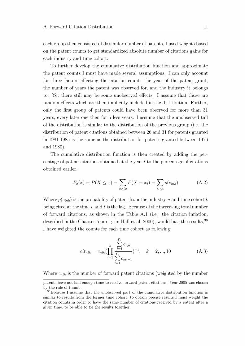
A. Forward Citation Distribution II
each group then consisted of dissimilar number of patents, I used weights based
on the patent counts to get standardized absolute number of citations gains for
each industry and time cohort.
To further develop the cumulative distribution function and approximate
the patent counts I must have made several assumptions. I can only account
for three factors affecting the citation count: the year of the patent grant,
the number of years the patent was observed for, and the industry it belongs
to. Yet there still may be some unobserved effects. I assume that those are
random effects which are then implicitly included in the distribution. Further,
only the first group of patents could have been observed for more than 31
years, every later one then for 5 less years. I assume that the unobserved tail
of the distribution is similar to the distribution of the previous group (i.e. the
distribution of patent citations obtained between 26 and 31 for patents granted
in 1981-1985 is the same as the distribution for patents granted between 1976
and 1980).
The cumulative distribution function is then created by adding the per-
centage of patent citations obtained at the year t to the percentage of citations
obtained earlier.
Fx(x) = P (X ≤ x) =∑xi≤x
P (X = xi) =∑ci≤t
p(cink) (A.2)
Where p(cink) is the probability of patent from the industry n and time cohort k
being cited at the time i, and t is the lag. Because of the increasing total number
of forward citations, as shown in the Table A.1 (i.e. the citation inflation,
described in the Chapter 5 or e.g. in Hall et al. 2000), would bias the results,36
I have weighted the counts for each time cohort as following:
citntk = cntk(k∏
i=1
Tk∑j=1
cnji
Tk∑l=1
cnli−1
)−1, k = 2, ..., 10 (A.3)
Where cntk is the number of forward patent citations (weighted by the number
patents have not had enough time to receive forward patent citations. Year 2005 was chosenby the rule of thumb.
36Because I assume that the unobserved part of the cumulative distribution function issimilar to results from the former time cohort, to obtain precise results I must weight thecitation counts in order to have the same number of citations received by a patent after agiven time, to be able to tie the results together.

A. Forward Citation Distribution III
of observed patents for the given time cohort) for each industry, year of grant,
and lag. Tk is the same for both sums in the numerator and the denominator,
it is the number of observed years in the time cohort i. These are divided by
the multiplication of all weights up to and including the time cohort k. In other
words, for k = 2 is the fraction equal to the sum of all citations gained by the
patents in the first time cohort up to and including lag T2, divided by the sum
of all citations received by the patents in the second time cohort (that is, again,
until the lag T2). For the next time cohort the fraction remains computed the
same way, but its result is further multiplied by the result of the fraction from
the first case.
In the end, the first time cohort remains the same, the second time cohort
is adjusted so the total number of citations gained within T2 years after the
patent grant is the same as in the first time cohort. The third is adjusted so
the total number of forward citations received within T3 years after the patent
grant is the same as the adjusted number of forward citations in the second
time cohort, and so on. Ultimately, I was able to tie the distribution from the
previous time cohort to the latter ones to obtain the cumulative distributions
for all patents with the year of grant from 1976 until 2005. These are depicted
in Figure A.1.
Figure A.1: Cumulative distribution functions for different time co-horts.
Even though there are visible fractures, the overall results are satisfactory.
One must keep in mind that the exact behaviour of the cumulative distribution

A. Forward Citation Distribution IV
functions more than 4 years after the tying is not important any more, because
it would only be used to predict forward citations for patents located close to
the tying.
Each patent in my dataset can be identified by its date of grant and industry
to its matching function. The predicted total number of citations a patent
would obtain through 31 years is then
total citations = observed citationsFnk(t)
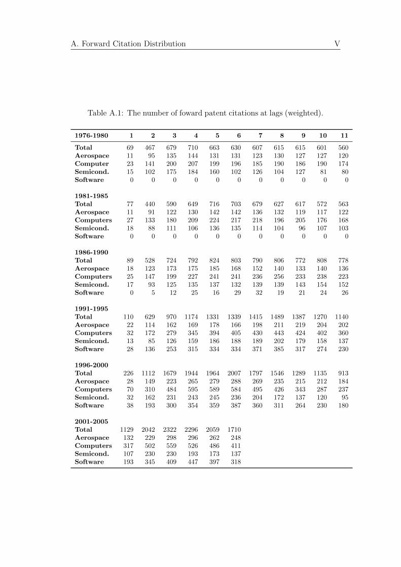
A. Forward Citation Distribution V
Table A.1: The number of foward patent citations at lags (weighted).
1976-1980 1 2 3 4 5 6 7 8 9 10 11
Total 69 467 679 710 663 630 607 615 615 601 560Aerospace 11 95 135 144 131 131 123 130 127 127 120Computer 23 141 200 207 199 196 185 190 186 190 174Semicond. 15 102 175 184 160 102 126 104 127 81 80Software 0 0 0 0 0 0 0 0 0 0 0
1981-1985Total 77 440 590 649 716 703 679 627 617 572 563Aerospace 11 91 122 130 142 142 136 132 119 117 122Computers 27 133 180 209 224 217 218 196 205 176 168Semicond. 18 88 111 106 136 135 114 104 96 107 103Software 0 0 0 0 0 0 0 0 0 0 0
1986-1990Total 89 528 724 792 824 803 790 806 772 808 778Aerospace 18 123 173 175 185 168 152 140 133 140 136Computers 25 147 199 227 241 241 236 256 233 238 223Semicond. 17 93 125 135 137 132 139 139 143 154 152Software 0 5 12 25 16 29 32 19 21 24 26
1991-1995Total 110 629 970 1174 1331 1339 1415 1489 1387 1270 1140Aerospace 22 114 162 169 178 166 198 211 219 204 202Computers 32 172 279 345 394 405 430 443 424 402 360Semicond. 13 85 126 159 186 188 189 202 179 158 137Software 28 136 253 315 334 334 371 385 317 274 230
1996-2000Total 226 1112 1679 1944 1964 2007 1797 1546 1289 1135 913Aerospace 28 149 223 265 279 288 269 235 215 212 184Computers 70 310 484 595 589 584 495 426 343 287 237Semicond. 32 162 231 243 245 236 204 172 137 120 95Software 38 193 300 354 359 387 360 311 264 230 180
2001-2005Total 1129 2042 2322 2296 2059 1710Aerospace 132 229 298 296 262 248Computers 317 502 559 526 486 411Semicond. 107 230 230 193 173 137Software 193 345 409 447 397 318

Appendix B
Data download
As it would be nearly impossible to collect such a large volume of data manually
from patent office databases, two other possible sources are available: commer-
cial on-line databases, allowing users to download bulk files, or web crawlers.
Commercial databases offer very fast services, often with advanced search for
precise needs; however, those are very expensive, limited in terms of provided
variables, or both. Web crawlers allow users to download exactly the data they
search for, but require a computer to run on and time to work.
For my study, I have used Easy Web Extract software.37 The program
crawls a given website and copies the selected parts (text, numbers, images),
based on set html objects, into the output file. The problem of the method is
the output file itself, as it only contains data as they appear on the website, not
in numerical form, which is preferred for latter use. Furthermore, if the website
is just poorly structured (i.e. a large part of the patent document shown on
the USPTO website is in plain text, not divided into separate parts or tables),
the program cannot download the requested data, simply because he cannot
distinguish them from the others. The only possibility how to obtain the data
then is to download the whole unstructured text and extract the right data
from it.
An average time of data download from one page is roughly 10 seconds;
however, this fully depends on the depth of the search. Given the large dataset
I decided to obtain and the fact that it had to be downloaded from two different
sources (repeatedly, due to new discoveries), the total time I spent downloading
was about 5 months.
37http://webextract.net
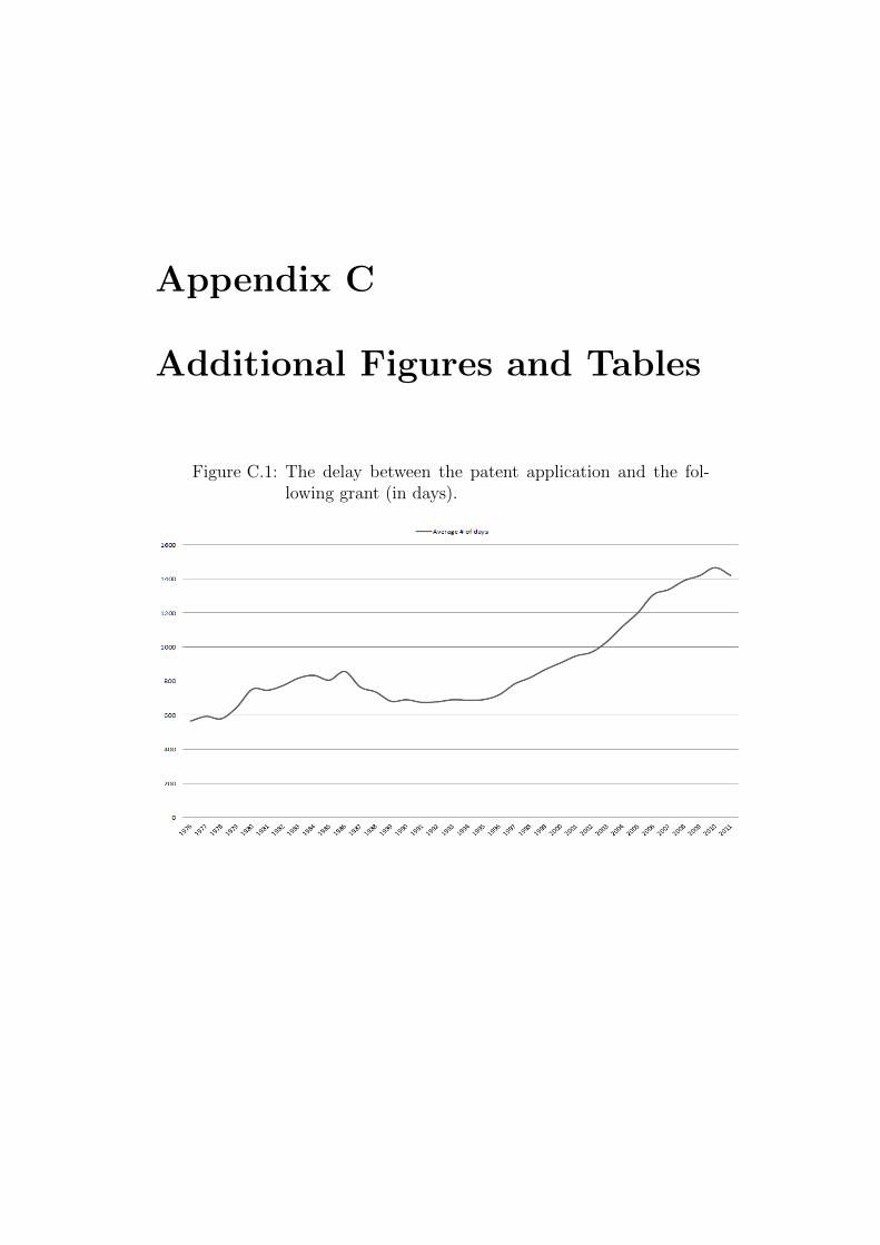
Appendix C
Additional Figures and Tables
Figure C.1: The delay between the patent application and the fol-lowing grant (in days).

C. Additional Figures and Tables VIII
Figure C.2: Renewal data, patents granted from 2000 to 2003.
Figure C.3: Renewal data, patents granted from 2004 to 2007.

C. Additional Figures and Tables IX
Figure C.4: Weighted forward citations by industry.
Figure C.5: Backward citations by industry.

C. Additional Figures and Tables X
Figure C.6: Family size by industry.
Figure C.7: Patent trades by industry.

C. Additional Figures and Tables XI
Table C.1: Companies overview.
Period Obs. F. Size F. Cit. Renewals Trades
Adobe 1989-2011 997 2.57 5.97 99.5% 9.7%AMD 1976-2011 9458 2.62 11.34 91.1% 25.7%Airbus 1991-2011 1375 5.54 2.63 98.0% 3.5%Altera 1986-2011 2055 3.06 9.37 98.7% 4.9%Apple 1978-2011 2986 4.02 12.64 99.8% 3.1%AM 1976-2011 5505 5.61 11.43 88.9% 2.6%Autodesk 1993-2011 392 3.54 4.96 96.9% 16.1%Boeing 1976-2011 7794 2.73 7.38 92.4% 3.9%CS 1998-2011 178 6.88 9.88 100.0% 1.1%Dell 1976-2011 2161 1.99 11.12 97.9% 1.6%Google 2003-2011 815 5.42 5.12 100.0% 4.5%HP 1992-2011 20166 3.09 8.43 97.2% 13.9%Intel 1976-2011 20306 3.12 9.47 94.7% 4.0%IBM 1976-2011 60251 2.86 9.62 81.4% 12.0%Intuit 1988-2011 221 1.56 3.05 93.8% 0.5%LTC 2010-2011 48 3.63 1.44 - -Logitech 1990-2011 221 5.57 10.57 93.5% 12.7%MIP 1987-2011 366 2.84 7.96 90.5% 6.8%Microsoft 1986-2011 16709 4.08 9.81 99.9% 1.5%NC 2000-2011 235 2.86 4.40 97.4% 69.8%Oracle 1995-2011 412 2.33 33.46 99.8% 8.3%Red Hat 2004-2011 200 1.73 0.95 100.0% 1.0%Symantec 1993-2011 929 3.21 5.82 100.0% 11.2%Textron 1976-2011 1712 4.97 9.08 85.7% 41.1%UT 1976-2011 5868 4.37 11.56 94.4% 10.2%
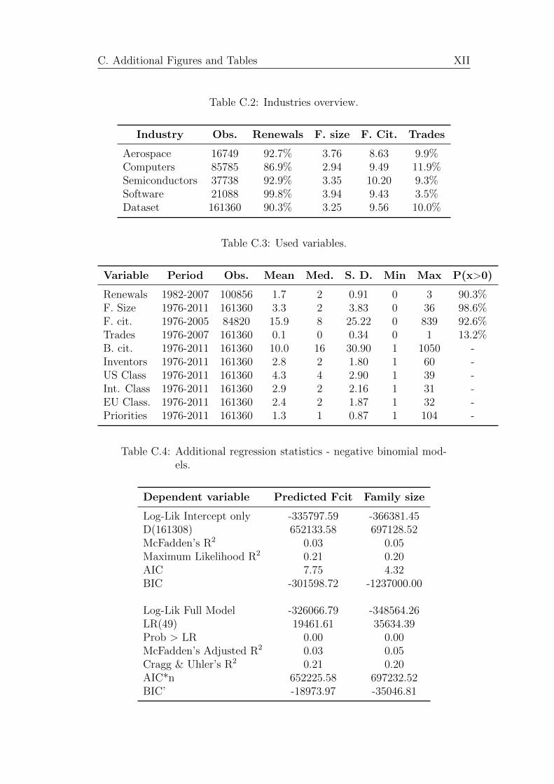
C. Additional Figures and Tables XII
Table C.2: Industries overview.
Industry Obs. Renewals F. size F. Cit. Trades
Aerospace 16749 92.7% 3.76 8.63 9.9%Computers 85785 86.9% 2.94 9.49 11.9%Semiconductors 37738 92.9% 3.35 10.20 9.3%Software 21088 99.8% 3.94 9.43 3.5%Dataset 161360 90.3% 3.25 9.56 10.0%
Table C.3: Used variables.
Variable Period Obs. Mean Med. S. D. Min Max P(x>0)
Renewals 1982-2007 100856 1.7 2 0.91 0 3 90.3%F. Size 1976-2011 161360 3.3 2 3.83 0 36 98.6%F. cit. 1976-2005 84820 15.9 8 25.22 0 839 92.6%Trades 1976-2007 161360 0.1 0 0.34 0 1 13.2%B. cit. 1976-2011 161360 10.0 16 30.90 1 1050 -Inventors 1976-2011 161360 2.8 2 1.80 1 60 -US Class 1976-2011 161360 4.3 4 2.90 1 39 -Int. Class 1976-2011 161360 2.9 2 2.16 1 31 -EU Class. 1976-2011 161360 2.4 2 1.87 1 32 -Priorities 1976-2011 161360 1.3 1 0.87 1 104 -
Table C.4: Additional regression statistics - negative binomial mod-els.
Dependent variable Predicted Fcit Family size
Log-Lik Intercept only -335797.59 -366381.45D(161308) 652133.58 697128.52McFadden’s R2 0.03 0.05Maximum Likelihood R2 0.21 0.20AIC 7.75 4.32BIC -301598.72 -1237000.00
Log-Lik Full Model -326066.79 -348564.26LR(49) 19461.61 35634.39Prob > LR 0.00 0.00McFadden’s Adjusted R2 0.03 0.05Cragg & Uhler’s R2 0.21 0.20AIC*n 652225.58 697232.52BIC’ -18973.97 -35046.81

C. Additional Figures and Tables XIII
Table C.5: Additional regression statistics - probit models.
Dependent variable Renewals Trades
Log-Lik Intercept Only -22628.17 -34558.40D(78987) 42043.24 66779.41McFadden’s R2 0.07 0.03Maximum Likelihood R2 0.04 0.03McKelvey and Zavoina’s R2 0.21 0.07Variance of y* 1.27 1.08Count R2 0.92 0.86AIC 0.53 0.80BIC -848738.19 -886930.20
Log-Lik Full Model -21021.62 -33389.71LR(37) 3213.10 2337.39Prob. > LR 0.00 0.00McFadden’s Adj R2 0.07 0.03Cragg & Uhler’s R2 0.09 0.05Efron’s R2 0.04 0.03Variance of error 1.00 1.00Adjusted Count R2 0.00 0.00AIC*n 42127.24 66875.41BIC’ -2795.83 -1838.41
Table C.6: Correlation matrix.
Fcit Fsize Trade RenewedFcit 1.00Fsize 0.07 1.00Trade 0.02 0.00 1.00Renewed 0.08 0.08 0.08 1.00

C. Additional Figures and Tables XIV
Table C.7: DEA variables (expenditures in $ millions).
Variable Obs. Mean Median St. D. Min Max
Employees Input 180 53775 12173 79101 163 319876R&D Expenditures Input 180 957 401 1251 3.78 5315# Patents Output 180 500 107 917 1 4425Composite Rating Output 180 3.69 3.98 1.06 0 5.85

C. Additional Figures and Tables XV
Table C.8: DEA analysis detailed results - software industry, bothoutcome variables.
Constant Returns to Scale
1994 1995 1996 1997 1998 1999 2000 2001 2002 2003
Adobe
100% 80% 84%91% 86% 87%
90% 88% 81%91% 82% 75%
89% 81% 77%81% 78% 71%
79% 73% 66%74% 68% 72%
100% 86% 86% 89% 84% 79% 78% 73% 67% 72%
Microsoft
85% 91% 94%86% 89% 90%
89% 90% 91%90% 91% 90%
95% 93% 91%94% 91% 85%
92% 85% 87%88% 90% 95%
85% 89% 90% 90% 92% 92% 91% 86% 89% 95%
Variable Returns to Scale
Adobe
100% 85% 85%97% 88% 87%
90% 91% 86%96% 89% 88%
90% 89% 88%91% 90% 90%
94% 95% 94%95% 94% 93%
100% 91% 88% 91% 88% 90% 91% 93% 94% 93%
Microsoft
87% 99% 100%100% 100% 100%
100% 100% 99%100% 99% 95%
100% 97% 92%100% 92% 87%
100% 86% 88%88% 90% 97%
87% 99% 100% 100% 100% 97% 95% 87% 89% 97%
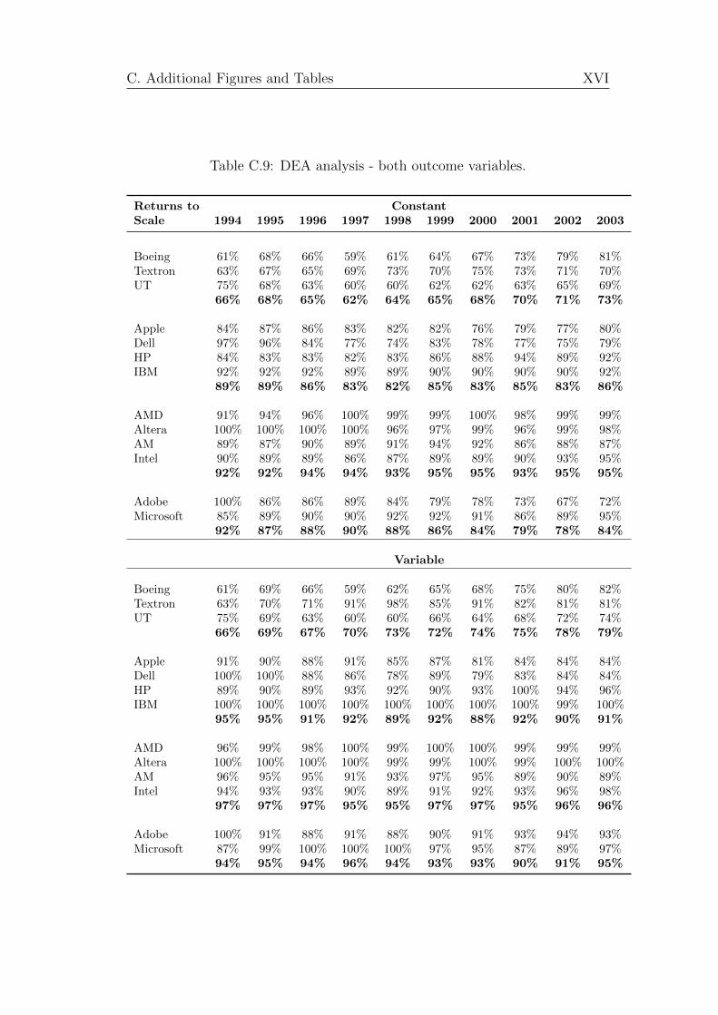
C. Additional Figures and Tables XVI
Table C.9: DEA analysis - both outcome variables.
Returns to ConstantScale 1994 1995 1996 1997 1998 1999 2000 2001 2002 2003
Boeing 61% 68% 66% 59% 61% 64% 67% 73% 79% 81%Textron 63% 67% 65% 69% 73% 70% 75% 73% 71% 70%UT 75% 68% 63% 60% 60% 62% 62% 63% 65% 69%
66% 68% 65% 62% 64% 65% 68% 70% 71% 73%
Apple 84% 87% 86% 83% 82% 82% 76% 79% 77% 80%Dell 97% 96% 84% 77% 74% 83% 78% 77% 75% 79%HP 84% 83% 83% 82% 83% 86% 88% 94% 89% 92%IBM 92% 92% 92% 89% 89% 90% 90% 90% 90% 92%
89% 89% 86% 83% 82% 85% 83% 85% 83% 86%
AMD 91% 94% 96% 100% 99% 99% 100% 98% 99% 99%Altera 100% 100% 100% 100% 96% 97% 99% 96% 99% 98%AM 89% 87% 90% 89% 91% 94% 92% 86% 88% 87%Intel 90% 89% 89% 86% 87% 89% 89% 90% 93% 95%
92% 92% 94% 94% 93% 95% 95% 93% 95% 95%
Adobe 100% 86% 86% 89% 84% 79% 78% 73% 67% 72%Microsoft 85% 89% 90% 90% 92% 92% 91% 86% 89% 95%
92% 87% 88% 90% 88% 86% 84% 79% 78% 84%
Variable
Boeing 61% 69% 66% 59% 62% 65% 68% 75% 80% 82%Textron 63% 70% 71% 91% 98% 85% 91% 82% 81% 81%UT 75% 69% 63% 60% 60% 66% 64% 68% 72% 74%
66% 69% 67% 70% 73% 72% 74% 75% 78% 79%
Apple 91% 90% 88% 91% 85% 87% 81% 84% 84% 84%Dell 100% 100% 88% 86% 78% 89% 79% 83% 84% 84%HP 89% 90% 89% 93% 92% 90% 93% 100% 94% 96%IBM 100% 100% 100% 100% 100% 100% 100% 100% 99% 100%
95% 95% 91% 92% 89% 92% 88% 92% 90% 91%
AMD 96% 99% 98% 100% 99% 100% 100% 99% 99% 99%Altera 100% 100% 100% 100% 99% 99% 100% 99% 100% 100%AM 96% 95% 95% 91% 93% 97% 95% 89% 90% 89%Intel 94% 93% 93% 90% 89% 91% 92% 93% 96% 98%
97% 97% 97% 95% 95% 97% 97% 95% 96% 96%
Adobe 100% 91% 88% 91% 88% 90% 91% 93% 94% 93%Microsoft 87% 99% 100% 100% 100% 97% 95% 87% 89% 97%
94% 95% 94% 96% 94% 93% 93% 90% 91% 95%

C. Additional Figures and Tables XVII
Table C.10: DEA analysis - patent numbers as the outcome variable.
Returns to ConstantScale 1994 1995 1996 1997 1998 1999 2000 2001 2002 2003
Boeing 54% 67% 66% 57% 58% 61% 61% 72% 79% 81%Textron 59% 60% 55% 54% 54% 58% 58% 58% 59% 62%UT 75% 68% 63% 60% 59% 57% 50% 55% 58% 66%
62% 65% 61% 57% 57% 59% 56% 62% 65% 70%
Apple 72% 81% 80% 72% 70% 70% 66% 72% 75% 80%Dell 97% 96% 82% 77% 71% 81% 72% 76% 72% 79%HP 81% 79% 81% 79% 79% 84% 87% 94% 89% 92%IBM 92% 92% 91% 89% 88% 90% 90% 90% 90% 92%
85% 87% 84% 79% 77% 81% 79% 83% 82% 86%
AMD 88% 90% 95% 100% 98% 98% 100% 98% 98% 97%Altera 96% 96% 94% 100% 96% 89% 78% 84% 91% 98%AM 83% 80% 84% 84% 85% 86% 87% 85% 88% 87%Intel 87% 86% 87% 85% 85% 88% 89% 90% 93% 95%
88% 88% 90% 92% 91% 90% 88% 89% 92% 94%
Adobe 37% 41% 63% 69% 68% 68% 68% 68% 67% 72%Microsoft 78% 81% 83% 83% 85% 86% 88% 86% 89% 95%
57% 61% 73% 76% 77% 77% 78% 77% 78% 84%
Variable
Boeing 60% 69% 66% 59% 60% 64% 66% 75% 80% 82%Textron 63% 64% 62% 62% 63% 65% 69% 75% 80% 81%UT 75% 69% 63% 60% 60% 61% 64% 68% 72% 74%
66% 67% 64% 60% 61% 63% 66% 73% 78% 79%
Apple 79% 86% 85% 80% 80% 81% 81% 84% 84% 84%Dell 97% 96% 83% 78% 72% 83% 78% 83% 84% 84%HP 81% 80% 82% 79% 80% 84% 90% 100% 94% 96%IBM 94% 97% 99% 99% 98% 100% 100% 99% 99% 100%
88% 90% 87% 84% 82% 87% 87% 92% 90% 91%
AMD 88% 92% 95% 100% 99% 99% 100% 99% 99% 98%Altera 100% 100% 100% 100% 99% 98% 96% 99% 100% 100%AM 86% 84% 88% 87% 89% 91% 90% 88% 90% 89%Intel 88% 87% 88% 85% 86% 89% 92% 93% 96% 98%
90% 91% 93% 93% 93% 94% 94% 95% 96% 96%
Adobe 88% 86% 87% 87% 88% 90% 91% 93% 94% 93%Microsoft 83% 84% 86% 86% 87% 88% 89% 87% 89% 97%
86% 85% 87% 87% 88% 89% 90% 90% 91% 95%

C. Additional Figures and Tables XVIII
Table C.11: DEA analysis - composite rating as the outcome variable.
Returns to ConstantScale 1994 1995 1996 1997 1998 1999 2000 2001 2002 2003
Boeing 47% 49% 52% 53% 55% 58% 60% 52% 54% 53%Textron 51% 60% 62% 69% 73% 70% 75% 70% 67% 67%UT 48% 50% 51% 54% 54% 61% 62% 57% 57% 58%
49% 53% 55% 59% 61% 63% 66% 60% 59% 60%
Apple 68% 65% 68% 81% 81% 82% 70% 67% 59% 40%Dell 76% 74% 73% 74% 73% 71% 68% 54% 60% 59%HP 53% 58% 57% 62% 63% 61% 58% 52% 46% 38%IBM 52% 54% 55% 53% 58% 54% 51% 44% 40% 30%
62% 63% 63% 68% 69% 67% 62% 54% 51% 42%
AMD 65% 67% 65% 64% 64% 67% 65% 69% 74% 84%Altera 100% 95% 94% 97% 93% 97% 99% 87% 86% 70%AM 71% 72% 72% 71% 75% 77% 69% 62% 65% 65%Intel 57% 60% 59% 60% 60% 59% 54% 50% 47% 39%
73% 74% 72% 73% 73% 75% 72% 67% 68% 65%
Adobe 100% 84% 82% 88% 84% 78% 69% 59% 40% 32%Microsoft 61% 72% 74% 78% 78% 74% 64% 59% 49% 26%
80% 78% 78% 83% 81% 76% 66% 59% 45% 29%
Variable
Boeing 56% 57% 56% 55% 57% 59% 62% 65% 69% 69%Textron 60% 64% 65% 88% 97% 85% 91% 82% 81% 81%UT 54% 55% 56% 57% 57% 64% 64% 68% 72% 74%
57% 59% 59% 67% 70% 69% 72% 72% 74% 74%
Apple 73% 70% 72% 86% 84% 87% 81% 83% 84% 84%Dell 78% 79% 76% 78% 76% 76% 74% 80% 84% 84%HP 58% 64% 61% 67% 68% 63% 64% 65% 64% 64%IBM 56% 59% 58% 55% 62% 56% 57% 59% 60% 60%
66% 68% 67% 71% 72% 70% 69% 72% 73% 73%
AMD 70% 72% 71% 73% 73% 75% 76% 78% 84% 85%Altera 100% 98% 98% 98% 99% 99% 100% 98% 100% 100%AM 76% 80% 76% 72% 77% 80% 74% 76% 78% 80%Intel 63% 64% 63% 62% 63% 64% 64% 66% 67% 67%
77% 78% 77% 76% 78% 79% 78% 80% 82% 83%
Adobe 100% 90% 87% 90% 88% 90% 91% 93% 94% 93%Microsoft 68% 85% 90% 95% 90% 85% 69% 69% 70% 69%
84% 88% 88% 92% 89% 88% 80% 81% 82% 81%