chemical non-equilibrium reentry flows in two … · chemical non-equilibrium reentry flows in...
TRANSCRIPT

Chemical Non-Equilibrium Reentry Flows in Two-Dimensions – Part II
EDISSON SÁVIO DE GÓES MACIEL(1)
AND AMILCAR PORTO PIMENTA(2)
IEA – Aeronautical Engineering Division
ITA – Aeronautical Technological Institute
Praça Mal. Eduardo Gomes, 50 – Vila das Acácias – São José dos Campos – SP – 12228-900
BRAZIL
, http://www.edissonsavio.eng.br(1)
and [email protected](2)
Abstract: - This work, second part of this study, presents two numerical tools implemented to simulate inviscid
and viscous flows employing the reactive gas formulation of thermal equilibrium and chemical non-
equilibrium. The Euler and Navier-Stokes equations, employing a finite volume formulation, on the context of
structured and unstructured spatial discretizations, are solved. The aerospace problems involving the hypersonic
flow around a blunt body, around a double ellipse, and around a re-entry capsule, in two-dimensions, are
simulated. The reactive simulations will involve an air chemical model of five species: N, N2, NO, O and O2.
Seventeen chemical reactions, involving dissociation and recombination, will be simulated by the proposed
model. The algorithms employed to solve the reactive equations were the Van Leer and the Liou and Steffen
Jr., first- and second-order accurate ones. The second-order numerical scheme is obtained by a “MUSCL”
(Monotone Upstream-centered Schemes for Conservation Laws) extrapolation process in the structured case.
The algorithms are accelerated to the steady state solution using a spatially variable time step procedure, which
has demonstrated effective gains in terms of convergence rate, as reported in Maciel. The results have
demonstrated that the most correct aerodynamic coefficient of lift to the re-entry problem is obtained by the
Van Leer first-order accurate scheme in the viscous, structured simulation. The Van Leer scheme is also the
most robust being able to simulate the major part of the studied problems.
Key-Words: - Euler and Navier-Stokes equations, Chemical non-equilibrium, Five species model,
Hypersonic flow, Van Leer algorithm, Liou and Steffen Jr. algorithm.
1 Introduction In several aerodynamic applications, the
atmospheric air, even being composed of several
chemical species, can be considered as a perfect
thermal and caloric gas due to its inert property as
well its uniform composition in space and constancy
in time. However, there are several practical
situations involving chemical reactions, as for
example: combustion processes, flows around
aerospace vehicles in re-entry conditions or plasma
flows, which do not permit the ideal gas hypothesis
([1]). As described in [2], since these chemical
reactions are very fast such that all processes can be
considered in equilibrium, the conservation laws
which govern the fluid become essentially
unaltered, except that one equation to the general
state of equilibrium has to be used opposed to the
ideal gas law. When the flow is not in chemical
equilibrium, one mass conservation law has to be
written to each chemical species and the size of the
equation system increases drastically.
To the motivation of the present work and to the
theoretical background to understand this one, the
reader is encouraged to read the first part of this
study [3]. This paper complements the present work
and finishes such study.
This work, second part of this study, presents
two numerical tools implemented to simulate
inviscid and viscous flows employing the reactive
gas formulation of thermal equilibrium and
chemical non-equilibrium flow in two-dimensions.
The Euler and Navier-Stokes equations, employing
a finite volume formulation, on the context of
structured and unstructured spatial discretizations,
are solved. These variants allow an effective
comparison between the two types of spatial
discretization aiming verify their potentialities:
solution quality, convergence speed, computational
cost, etc. The aerospace problems involving the “hot
gas” hypersonic flow around a blunt body, around a
double ellipse, and around a re-entry capsule in two-
dimensions, are simulated. The algorithms are
accelerated to the steady state solution using a
spatially variable time step procedure, which has
demonstrated effective gains in terms of
convergence rate, as shown in [4-5].
The reactive simulations will involve an air
chemical model of five species: N, O, N2, O2 and
NO. Seventeen chemical reactions, involving
dissociation and recombination, will be simulated
WSEAS TRANSACTIONS on FLUID MECHANICS Edisson Sávio De Góes Maciel, Amilcar Porto Pimenta
E-ISSN: 2224-347X 50 Issue 2, Volume 8, April 2013
by the proposed model. The Arrhenius formula will
be employed to determine the reaction rates and the
law of mass action will be used to determine the
source terms of each gas species equation.
The algorithms employed to solve the reactive
equations were the [6-7], first- and second-order
accurate ones. The second-order numerical scheme
is obtained by a MUSCL extrapolation process in
the structured case. In the unstructured case, tests
with the linear reconstruction process did not yield
converged results and, therefore, were not
presented. Only first-order solutions are presented.
The algorithm was implemented in a FORTRAN
programming language, using the software
Microsoft Developer Studio. Simulations in a
notebook with processor PENTIUM INTEL Duo
Core 2.30 GHz of clock and 2 GBytes of RAM were
performed.
The results have demonstrated that the most
correct aerodynamic coefficient of lift, to the re-
entry capsule, is obtained by the [6] first-order
accurate scheme in the viscous and structured
simulation. Moreover, the [6] scheme is also the
most robust being able to simulate the major part of
the studied problems
2 Unstructured Formulation and the
Liou and Steffen Jr. Scheme The Euler and Navier-Stokes equations are
presented in details in [3] and because it is not
presented here again. The thermodynamic and
transport properties are also described in [3], as well
the chemical formulation, and are not repeated
herein. Only the unstructured formulation and the
[7] algorithm were not presented and are detailed in
this work.
2.1. Unstructured formulation
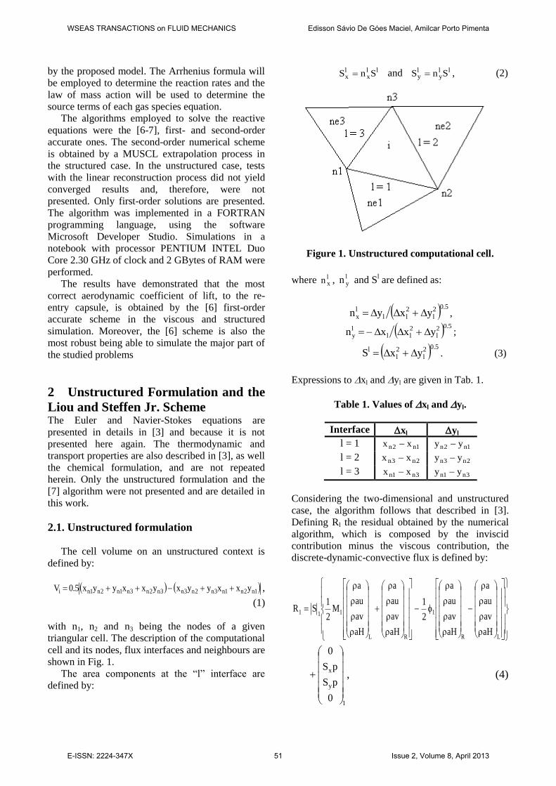
The cell volume on an unstructured context is
defined by:
1n2n1n3n2n3n3n2n3n1n2n1ni yxxyyxyxxyyx5.0V ,
(1)
with n1, n2 and n3 being the nodes of a given
triangular cell. The description of the computational
cell and its nodes, flux interfaces and neighbours are
shown in Fig. 1.
The area components at the “l” interface are
defined by:
llx
lx SnS and ll
yly SnS , (2)
Figure 1. Unstructured computational cell.
where lxn , l
yn and Sl are defined as:
5.02l
2ll
lx yxyn ,
5.02l
2ll
ly yxxn ;
5.02l
2l
l yxS . (3)
Expressions to xl and yl are given in Tab. 1.
Table 1. Values of xl and yl.
Interface xl yl
l = 1 1n2n xx 1n2n yy
l = 2 2n3n xx 2n3n yy
l = 3 3n1n xx 3n1n yy
Considering the two-dimensional and unstructured
case, the algorithm follows that described in [3].
Defining Rl the residual obtained by the numerical
algorithm, which is composed by the inviscid
contribution minus the viscous contribution, the
discrete-dynamic-convective flux is defined by:
LR
1
RL
111
aH
av
au
a
aH
av
au
a
2
1
aH
av
au
a
aH
av
au
a
M2
1SR
1
y
x
0
pS
pS
0
, (4)
WSEAS TRANSACTIONS on FLUID MECHANICS Edisson Sávio De Góes Maciel, Amilcar Porto Pimenta
E-ISSN: 2224-347X 51 Issue 2, Volume 8, April 2013
and the discrete-chemical-convective flux is defined
by:
L5
4
2
1
R5
4
2
1
1
R5
4
2
1
L5
4
2
1
111
a
a
a
a
a
a
a
a
2
1
a
a
a
a
a
a
a
a
M2
1SR ,
(5)
The time integration is performed by the Runge-
Kutta explicit method of five stages, second-order
accurate, to the two types of convective flux. To the
dynamic part, this method can be represented in
general form by:
)k(
i
)1n(
i
i
)1k(
iik
)0(
i
)k(
i
)n(
i
)0(
i
VQRtQQ
, (6)
and to the chemical part, it can be represented in
general form by:
)k(
i
)1n(
i
)1k(
iCi
)1k(
iik
)0(
i
)k(
i
)n(
i
)0(
i
QSVQRtQQ
, (7)
where the chemical source term SC is calculated
with the translational/rotational temperature, k =
1,...,5; 1 = 1/4, 2 = 1/6, 3 = 3/8, 4 = 1/2 and 5
= 1.
2.2. Liou and Steffen Jr. algorithm
The appropriated choice of the l term defines the
[7] scheme according to [8]. Hence, the following
definition describes the [7] scheme:
ll M or j,2/1ij,2/1i M , (8)
for unstructured and structured cases, respectively.
The viscous formulation follows that of [9],
which adopts the Green theorem to calculate
primitive variable gradients. The viscous vectors are
obtained by arithmetical average of flow properties
between cell (i,j) and its neighbors. As was done
with the convective terms, there is a need to separate
the viscous flux in two parts: dynamical viscous flux
and chemical viscous flux. The dynamical part
corresponds to the first four equations of the Navier-
Stokes ones and the chemical part corresponds to
the last four equations.
A spatially variable time step procedure was
employed aiming to accelerate the convergence of
the numerical schemes. This technique has provided
excellent convergence gains as demonstrated in [4-
5] and is implemented in the present codes.
3 Results Four (4) orders of reduction of the maximum
residual were adopted as convergence criterion. In
the simulations, the attack angle was set equal to
zero.
3.1 Initial and boundary conditions to the
studied problem The initial conditions are presented in Table 2. The
Reynolds number is obtained from data of [10]. The
boundary conditions to this problem of reactive flow
are detailed in [11], as well the blunt body
geometry, the meshes employed in the simulations
and the description of the computational
configuration. As aforementioned, the first
geometry is a blunt body with 1.0 m of nose ratio
and parallel rectilinear walls. The far field is located
at 20.0 times the nose ratio in relation to the
configuration nose.
Table 2. Initial conditions to the problem of the
blunt body.
Property Value
M 8.78
0.00326 kg/m3
p 687.0 Pa
U 4,776 m/s
T 694.0 K
Altitude 40,000 m
cN 10-9
cO 0.07955
cO2 0.13400
cNO 0.05090
L 2.0 m
Re 2.3885x10⁶
3.2. Blunt body results
3.2.1. Inviscid, unstructured and first-order
accurate case – Same sense
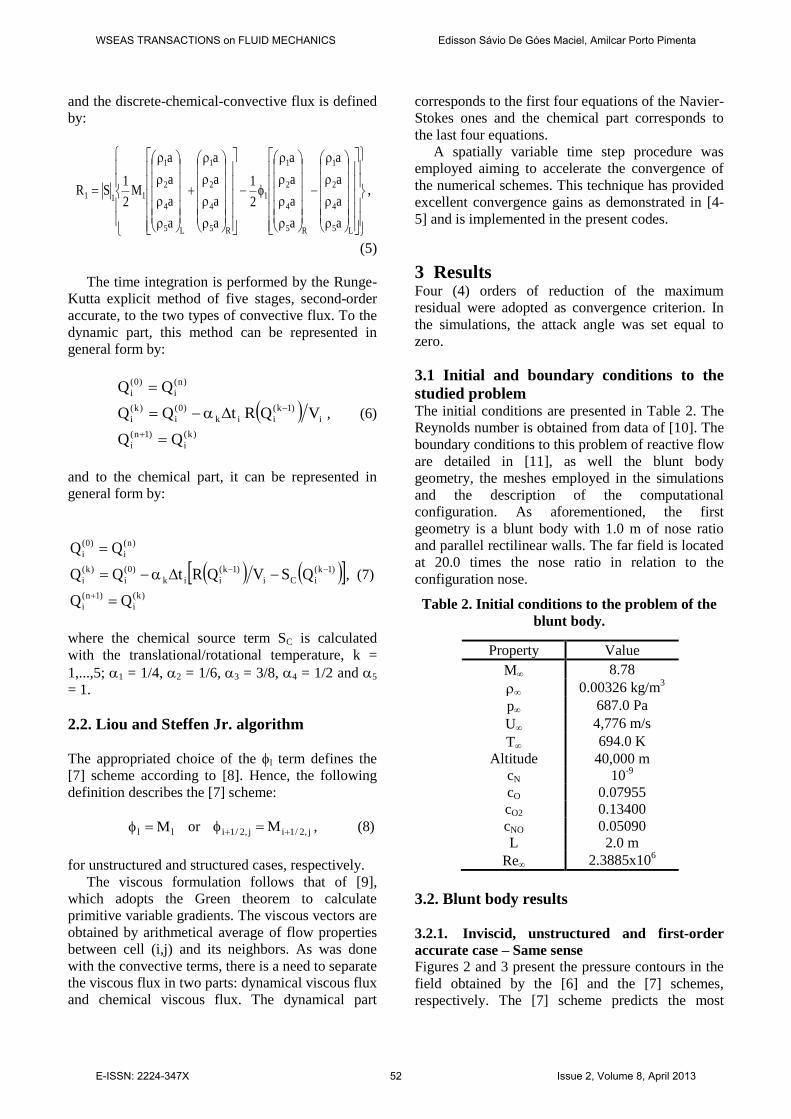
Figures 2 and 3 present the pressure contours in the
field obtained by the [6] and the [7] schemes,
respectively. The [7] scheme predicts the most
WSEAS TRANSACTIONS on FLUID MECHANICS Edisson Sávio De Góes Maciel, Amilcar Porto Pimenta
E-ISSN: 2224-347X 52 Issue 2, Volume 8, April 2013
severe pressure peak of approximately 159 unities.
The [6] solution shows good symmetry properties.
There are not pre- or post-shock oscillations.
Figure 2. Pressure Contours (VL).
Figure 3. Pressure Contours (LS).
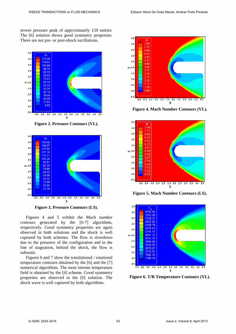
Figures 4 and 5 exhibit the Mach number
contours generated by the [6-7] algorithms,
respectively. Good symmetry properties are again
observed in both solutions and the shock is well
captured by both schemes. The flow is slowdown
due to the presence of the configuration and in the
line of stagnation, behind the shock, the flow is
subsonic.
Figures 6 and 7 show the translational / rotational
temperature contours obtained by the [6] and the [7]
numerical algorithms. The most intense temperature
field is obtained by the [6] scheme. Good symmetry
properties are observed in the [6] solution. The
shock wave is well captured by both algorithms.
Figure 4. Mach Number Contours (VL).
Figure 5. Mach Number Contours (LS).
Figure 6. T/R Temperature Contours (VL).
WSEAS TRANSACTIONS on FLUID MECHANICS Edisson Sávio De Góes Maciel, Amilcar Porto Pimenta
E-ISSN: 2224-347X 53 Issue 2, Volume 8, April 2013

Figure 7. T/R Temperature Contours (LS).
Figure 8. Velocity Vector Field (VL).
Figure 9. Velocity Vector Field (LS).
Figure 8 and 9 present the flow velocity vector
field generated by the [6] and the [7] numerical
schemes, respectively. The shock wave is well
captured, good symmetry properties are observed
and the tangency and impermeability conditions are
well satisfied.
3.2.2. Viscous, unstructured and first-order
accurate case – Same sense
Figures 10 and 11 exhibit the pressure contours
obtained by the [6-7] schemes, respectively. The
most severe pressure field is generated by the [6]
scheme, with a pressure peak of approximately 166
unities. Better symmetry properties than in the
inviscid case are observed in both solutions.
Figure 10. Pressure Contours (VL).
Figure 11. Pressure Contours (LS).
Figures 12 and 13 show the Mach number
contours obtained by the [6] and the [7] numerical
schemes, respectively. The Mach number field
generated by the [7] algorithm is more intense than
that generated by the [6] algorithm. Good symmetry
properties are observed in both solutions. The shock
wave is well captured by both schemes. The Mach
wave develops naturally: passing from a normal
shock wave at the blunt nose to oblique shock
waves close to the body and to Mach waves far from
WSEAS TRANSACTIONS on FLUID MECHANICS Edisson Sávio De Góes Maciel, Amilcar Porto Pimenta
E-ISSN: 2224-347X 54 Issue 2, Volume 8, April 2013
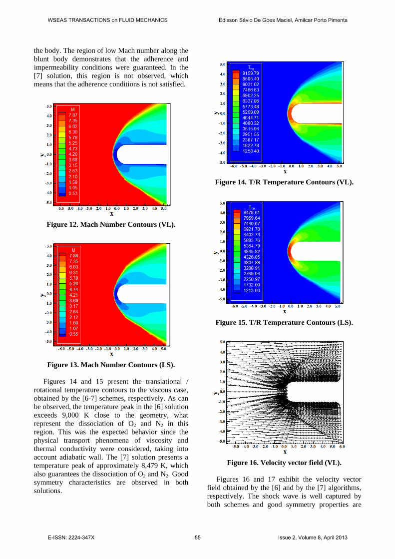
the body. The region of low Mach number along the
blunt body demonstrates that the adherence and
impermeability conditions were guaranteed. In the
[7] solution, this region is not observed, which
means that the adherence conditions is not satisfied.
Figure 12. Mach Number Contours (VL).
Figure 13. Mach Number Contours (LS).
Figures 14 and 15 present the translational /
rotational temperature contours to the viscous case,
obtained by the [6-7] schemes, respectively. As can
be observed, the temperature peak in the [6] solution
exceeds 9,000 K close to the geometry, what
represent the dissociation of O2 and N2 in this
region. This was the expected behavior since the
physical transport phenomena of viscosity and
thermal conductivity were considered, taking into
account adiabatic wall. The [7] solution presents a
temperature peak of approximately 8,479 K, which
also guarantees the dissociation of O2 and N2. Good
symmetry characteristics are observed in both
solutions.
Figure 14. T/R Temperature Contours (VL).
Figure 15. T/R Temperature Contours (LS).
Figure 16. Velocity vector field (VL).
Figures 16 and 17 exhibit the velocity vector
field obtained by the [6] and by the [7] algorithms,
respectively. The shock wave is well captured by
both schemes and good symmetry properties are
WSEAS TRANSACTIONS on FLUID MECHANICS Edisson Sávio De Góes Maciel, Amilcar Porto Pimenta
E-ISSN: 2224-347X 55 Issue 2, Volume 8, April 2013
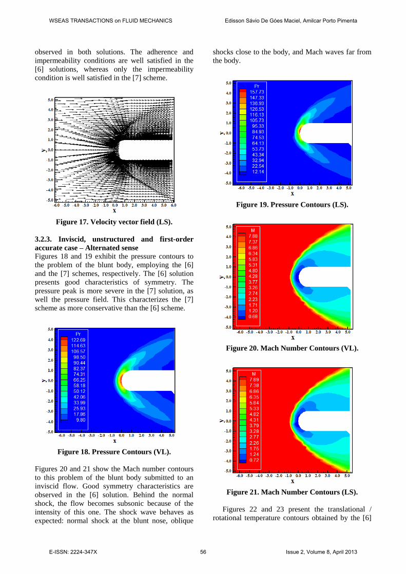
observed in both solutions. The adherence and
impermeability conditions are well satisfied in the
[6] solutions, whereas only the impermeability
condition is well satisfied in the [7] scheme.
Figure 17. Velocity vector field (LS).
3.2.3. Inviscid, unstructured and first-order
accurate case – Alternated sense Figures 18 and 19 exhibit the pressure contours to
the problem of the blunt body, employing the [6]
and the [7] schemes, respectively. The [6] solution
presents good characteristics of symmetry. The
pressure peak is more severe in the [7] solution, as
well the pressure field. This characterizes the [7]
scheme as more conservative than the [6] scheme.
Figure 18. Pressure Contours (VL).
Figures 20 and 21 show the Mach number contours
to this problem of the blunt body submitted to an
inviscid flow. Good symmetry characteristics are
observed in the [6] solution. Behind the normal
shock, the flow becomes subsonic because of the
intensity of this one. The shock wave behaves as
expected: normal shock at the blunt nose, oblique
shocks close to the body, and Mach waves far from
the body.
Figure 19. Pressure Contours (LS).
Figure 20. Mach Number Contours (VL).
Figure 21. Mach Number Contours (LS).
Figures 22 and 23 present the translational /
rotational temperature contours obtained by the [6]
WSEAS TRANSACTIONS on FLUID MECHANICS Edisson Sávio De Góes Maciel, Amilcar Porto Pimenta
E-ISSN: 2224-347X 56 Issue 2, Volume 8, April 2013
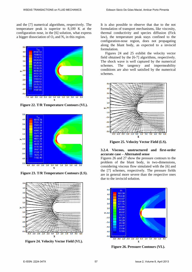
and the [7] numerical algorithms, respectively. The
temperature peak is superior to 8,100 K at the
configuration nose, in the [6] solution, what express
a bigger dissociation of O2 and N2 in this region.
Figure 22. T/R Temperature Contours (VL).
Figure 23. T/R Temperature Contours (LS).
Figure 24. Velocity Vector Field (VL).
It is also possible to observe that due to the not
formulation of transport mechanisms, like viscosity,
thermal conductivity and species diffusion (Fick
law), the temperature peak stays confined to the
configuration-nose region, does not propagating
along the blunt body, as expected to a inviscid
formulation.
Figures 24 and 25 exhibit the velocity vector
field obtained by the [6-7] algorithms, respectively.
The shock wave is well captured by the numerical
schemes. The tangency and impermeability
conditions are also well satisfied by the numerical
schemes.
Figure 25. Velocity Vector Field (LS).
3.2.4. Viscous, unstructured and first-order
accurate case – Alternated sense Figures 26 and 27 show the pressure contours to the
problem of the blunt body, in two-dimensions,
considering viscous flow simulated with the [6] and
the [7] schemes, respectively. The pressure fields
are in general more severe than the respective ones
due to the inviscid solution.
Figure 26. Pressure Contours (VL).
WSEAS TRANSACTIONS on FLUID MECHANICS Edisson Sávio De Góes Maciel, Amilcar Porto Pimenta
E-ISSN: 2224-347X 57 Issue 2, Volume 8, April 2013
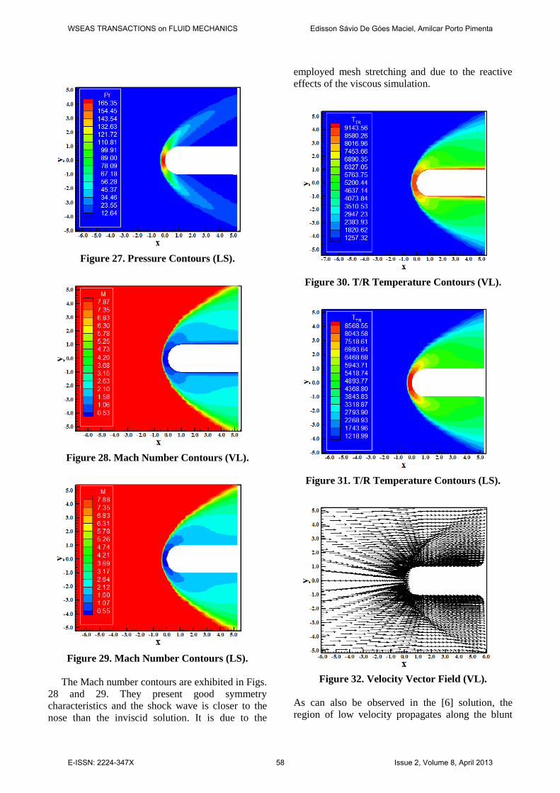
Figure 27. Pressure Contours (LS).
Figure 28. Mach Number Contours (VL).
Figure 29. Mach Number Contours (LS).
The Mach number contours are exhibited in Figs.
28 and 29. They present good symmetry
characteristics and the shock wave is closer to the
nose than the inviscid solution. It is due to the
employed mesh stretching and due to the reactive
effects of the viscous simulation.
Figure 30. T/R Temperature Contours (VL).
Figure 31. T/R Temperature Contours (LS).
Figure 32. Velocity Vector Field (VL).
As can also be observed in the [6] solution, the
region of low velocity propagates along the blunt
WSEAS TRANSACTIONS on FLUID MECHANICS Edisson Sávio De Góes Maciel, Amilcar Porto Pimenta
E-ISSN: 2224-347X 58 Issue 2, Volume 8, April 2013
body, satisfying the conditions of adherence and
impermeability of the viscous formulation. The
same is not true to the [7] solution.
Figures 30 and 31 present the translational /
rotational temperature distribution in the
computational domain generated by the [6-7]
schemes, respectively. The translational / rotational
temperature peak is approximately 9,144 K to the
[6] scheme and 8,569 K to the [7] scheme. The
influence of the translational / rotational temperature
is confined to a very much restrict region, which
corresponds to the boundary layer, due to the
consideration of the transport phenomena (viscosity,
thermal conductivity and species diffusion).
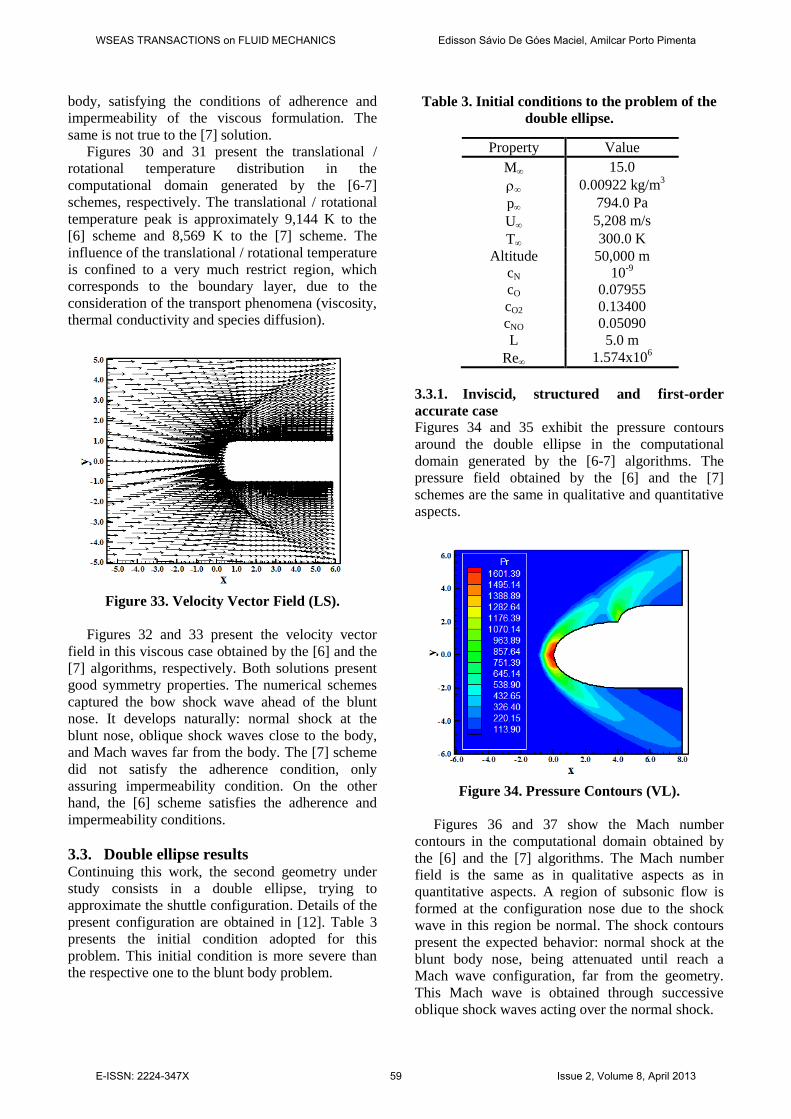
Figure 33. Velocity Vector Field (LS).
Figures 32 and 33 present the velocity vector
field in this viscous case obtained by the [6] and the
[7] algorithms, respectively. Both solutions present
good symmetry properties. The numerical schemes
captured the bow shock wave ahead of the blunt
nose. It develops naturally: normal shock at the
blunt nose, oblique shock waves close to the body,
and Mach waves far from the body. The [7] scheme
did not satisfy the adherence condition, only
assuring impermeability condition. On the other
hand, the [6] scheme satisfies the adherence and
impermeability conditions.
3.3. Double ellipse results Continuing this work, the second geometry under
study consists in a double ellipse, trying to
approximate the shuttle configuration. Details of the
present configuration are obtained in [12]. Table 3
presents the initial condition adopted for this
problem. This initial condition is more severe than
the respective one to the blunt body problem.
Table 3. Initial conditions to the problem of the
double ellipse.
Property Value
M 15.0
0.00922 kg/m3
p 794.0 Pa
U 5,208 m/s
T 300.0 K
Altitude 50,000 m
cN 10-9
cO 0.07955
cO2 0.13400
cNO 0.05090
L 5.0 m
Re 1.574x10⁶
3.3.1. Inviscid, structured and first-order
accurate case Figures 34 and 35 exhibit the pressure contours
around the double ellipse in the computational
domain generated by the [6-7] algorithms. The
pressure field obtained by the [6] and the [7]
schemes are the same in qualitative and quantitative
aspects.
Figure 34. Pressure Contours (VL).
Figures 36 and 37 show the Mach number
contours in the computational domain obtained by
the [6] and the [7] algorithms. The Mach number
field is the same as in qualitative aspects as in
quantitative aspects. A region of subsonic flow is
formed at the configuration nose due to the shock
wave in this region be normal. The shock contours
present the expected behavior: normal shock at the
blunt body nose, being attenuated until reach a
Mach wave configuration, far from the geometry.
This Mach wave is obtained through successive
oblique shock waves acting over the normal shock.
WSEAS TRANSACTIONS on FLUID MECHANICS Edisson Sávio De Góes Maciel, Amilcar Porto Pimenta
E-ISSN: 2224-347X 59 Issue 2, Volume 8, April 2013
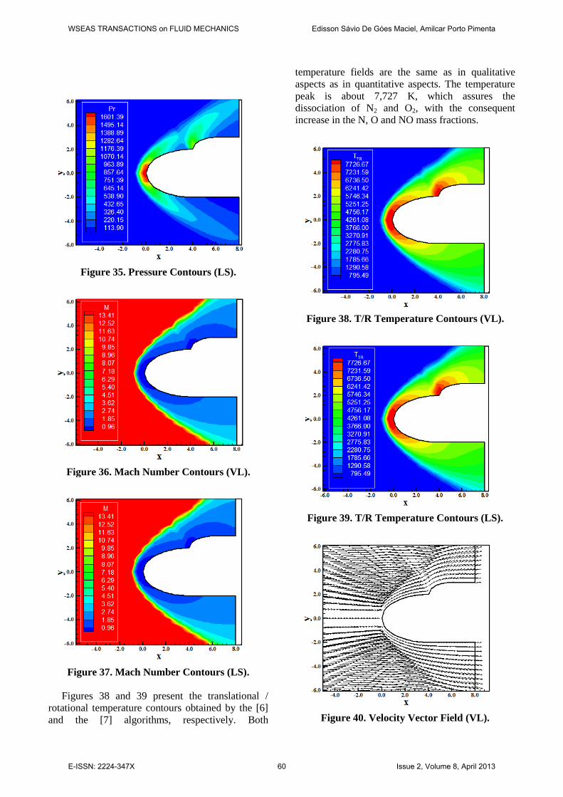
Figure 35. Pressure Contours (LS).
Figure 36. Mach Number Contours (VL).
Figure 37. Mach Number Contours (LS).
Figures 38 and 39 present the translational /
rotational temperature contours obtained by the [6]
and the [7] algorithms, respectively. Both
temperature fields are the same as in qualitative
aspects as in quantitative aspects. The temperature
peak is about 7,727 K, which assures the
dissociation of N2 and O2, with the consequent
increase in the N, O and NO mass fractions.
Figure 38. T/R Temperature Contours (VL).
Figure 39. T/R Temperature Contours (LS).
Figure 40. Velocity Vector Field (VL).
WSEAS TRANSACTIONS on FLUID MECHANICS Edisson Sávio De Góes Maciel, Amilcar Porto Pimenta
E-ISSN: 2224-347X 60 Issue 2, Volume 8, April 2013
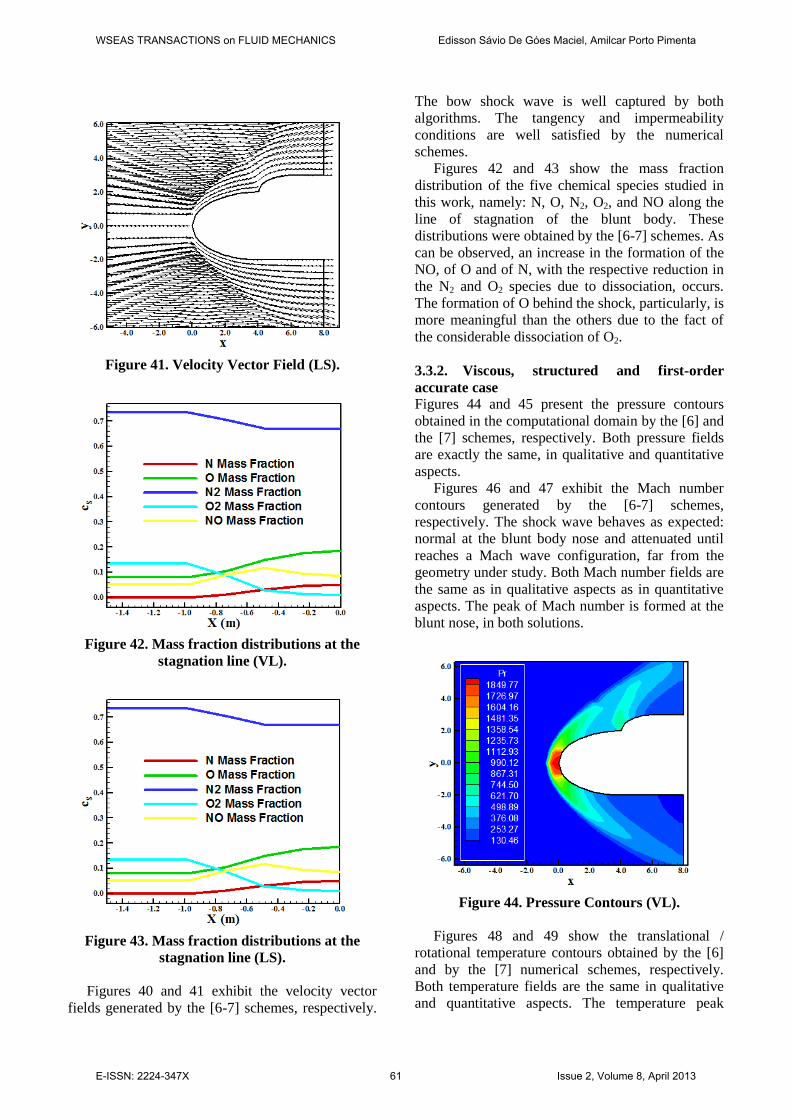
Figure 41. Velocity Vector Field (LS).
Figure 42. Mass fraction distributions at the
stagnation line (VL).
Figure 43. Mass fraction distributions at the
stagnation line (LS).
Figures 40 and 41 exhibit the velocity vector
fields generated by the [6-7] schemes, respectively.
The bow shock wave is well captured by both
algorithms. The tangency and impermeability
conditions are well satisfied by the numerical
schemes.
Figures 42 and 43 show the mass fraction
distribution of the five chemical species studied in
this work, namely: N, O, N2, O2, and NO along the
line of stagnation of the blunt body. These
distributions were obtained by the [6-7] schemes. As
can be observed, an increase in the formation of the
NO, of O and of N, with the respective reduction in
the N2 and O2 species due to dissociation, occurs.
The formation of O behind the shock, particularly, is
more meaningful than the others due to the fact of
the considerable dissociation of O2.
3.3.2. Viscous, structured and first-order
accurate case Figures 44 and 45 present the pressure contours
obtained in the computational domain by the [6] and
the [7] schemes, respectively. Both pressure fields
are exactly the same, in qualitative and quantitative
aspects.
Figures 46 and 47 exhibit the Mach number
contours generated by the [6-7] schemes,
respectively. The shock wave behaves as expected:
normal at the blunt body nose and attenuated until
reaches a Mach wave configuration, far from the
geometry under study. Both Mach number fields are
the same as in qualitative aspects as in quantitative
aspects. The peak of Mach number is formed at the
blunt nose, in both solutions.
Figure 44. Pressure Contours (VL).
Figures 48 and 49 show the translational /
rotational temperature contours obtained by the [6]
and by the [7] numerical schemes, respectively.
Both temperature fields are the same in qualitative
and quantitative aspects. The temperature peak
WSEAS TRANSACTIONS on FLUID MECHANICS Edisson Sávio De Góes Maciel, Amilcar Porto Pimenta
E-ISSN: 2224-347X 61 Issue 2, Volume 8, April 2013
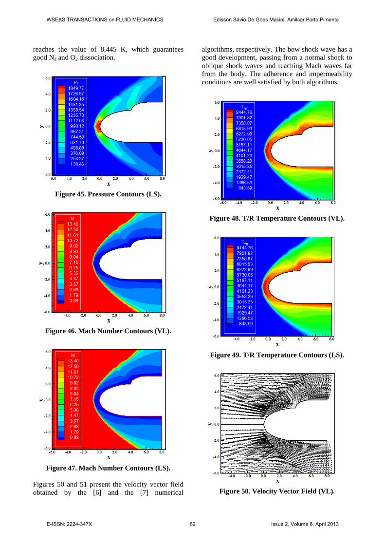
reaches the value of 8,445 K, which guarantees
good N2 and O2 dissociation.
Figure 45. Pressure Contours (LS).
Figure 46. Mach Number Contours (VL).
Figure 47. Mach Number Contours (LS).
Figures 50 and 51 present the velocity vector field
obtained by the [6] and the [7] numerical
algorithms, respectively. The bow shock wave has a
good development, passing from a normal shock to
oblique shock waves and reaching Mach waves far
from the body. The adherence and impermeability
conditions are well satisfied by both algorithms.
Figure 48. T/R Temperature Contours (VL).
Figure 49. T/R Temperature Contours (LS).
Figure 50. Velocity Vector Field (VL).
WSEAS TRANSACTIONS on FLUID MECHANICS Edisson Sávio De Góes Maciel, Amilcar Porto Pimenta
E-ISSN: 2224-347X 62 Issue 2, Volume 8, April 2013
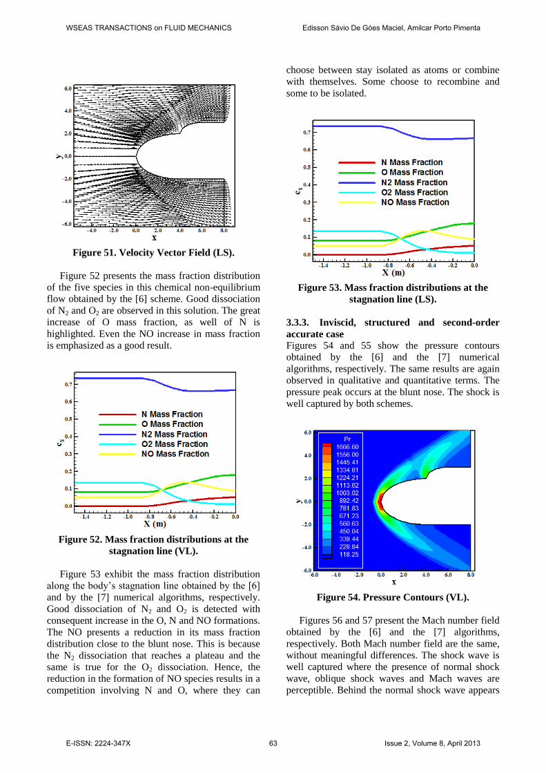
Figure 51. Velocity Vector Field (LS).
Figure 52 presents the mass fraction distribution
of the five species in this chemical non-equilibrium
flow obtained by the [6] scheme. Good dissociation
of N2 and O2 are observed in this solution. The great
increase of O mass fraction, as well of N is
highlighted. Even the NO increase in mass fraction
is emphasized as a good result.
Figure 52. Mass fraction distributions at the
stagnation line (VL).
Figure 53 exhibit the mass fraction distribution
along the body’s stagnation line obtained by the [6]
and by the [7] numerical algorithms, respectively.
Good dissociation of N2 and O2 is detected with
consequent increase in the O, N and NO formations.
The NO presents a reduction in its mass fraction
distribution close to the blunt nose. This is because
the N2 dissociation that reaches a plateau and the
same is true for the O2 dissociation. Hence, the
reduction in the formation of NO species results in a
competition involving N and O, where they can
choose between stay isolated as atoms or combine
with themselves. Some choose to recombine and
some to be isolated.
Figure 53. Mass fraction distributions at the
stagnation line (LS).
3.3.3. Inviscid, structured and second-order
accurate case
Figures 54 and 55 show the pressure contours
obtained by the [6] and the [7] numerical
algorithms, respectively. The same results are again
observed in qualitative and quantitative terms. The
pressure peak occurs at the blunt nose. The shock is
well captured by both schemes.
Figure 54. Pressure Contours (VL).
Figures 56 and 57 present the Mach number field
obtained by the [6] and the [7] algorithms,
respectively. Both Mach number field are the same,
without meaningful differences. The shock wave is
well captured where the presence of normal shock
wave, oblique shock waves and Mach waves are
perceptible. Behind the normal shock wave appears
WSEAS TRANSACTIONS on FLUID MECHANICS Edisson Sávio De Góes Maciel, Amilcar Porto Pimenta
E-ISSN: 2224-347X 63 Issue 2, Volume 8, April 2013
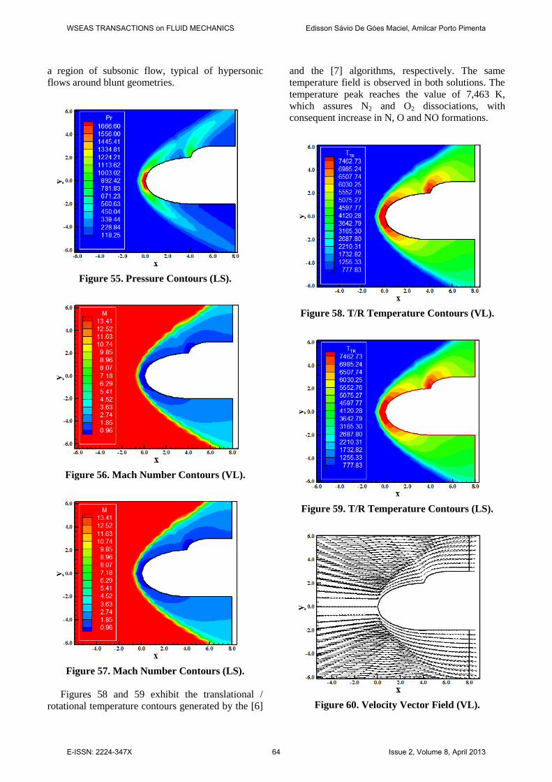
a region of subsonic flow, typical of hypersonic
flows around blunt geometries.
Figure 55. Pressure Contours (LS).
Figure 56. Mach Number Contours (VL).
Figure 57. Mach Number Contours (LS).
Figures 58 and 59 exhibit the translational /
rotational temperature contours generated by the [6]
and the [7] algorithms, respectively. The same
temperature field is observed in both solutions. The
temperature peak reaches the value of 7,463 K,
which assures N2 and O2 dissociations, with
consequent increase in N, O and NO formations.
Figure 58. T/R Temperature Contours (VL).
Figure 59. T/R Temperature Contours (LS).
Figure 60. Velocity Vector Field (VL).
WSEAS TRANSACTIONS on FLUID MECHANICS Edisson Sávio De Góes Maciel, Amilcar Porto Pimenta
E-ISSN: 2224-347X 64 Issue 2, Volume 8, April 2013
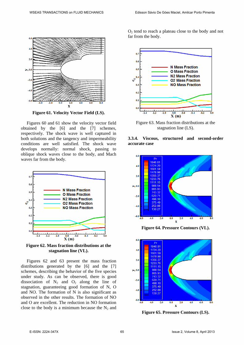
Figure 61. Velocity Vector Field (LS).
Figures 60 and 61 show the velocity vector field
obtained by the [6] and the [7] schemes,
respectively. The shock wave is well captured in
both solutions and the tangency and impermeability
conditions are well satisfied. The shock wave
develops normally: normal shock, passing to
oblique shock waves close to the body, and Mach
waves far from the body.
Figure 62. Mass fraction distributions at the
stagnation line (VL).
Figures 62 and 63 present the mass fraction
distributions generated by the [6] and the [7]
schemes, describing the behavior of the five species
under study. As can be observed, there is good
dissociation of N2 and O2 along the line of
stagnation, guaranteeing good formation of N, O
and NO. The formation of N is also significant as
observed in the other results. The formation of NO
and O are excellent. The reduction in NO formation
close to the body is a minimum because the N2 and
O2 tend to reach a plateau close to the body and not
far from the body.
Figure 63. Mass fraction distributions at the
stagnation line (LS).
3.3.4. Viscous, structured and second-order
accurate case
Figure 64. Pressure Contours (VL).
Figure 65. Pressure Contours (LS).
WSEAS TRANSACTIONS on FLUID MECHANICS Edisson Sávio De Góes Maciel, Amilcar Porto Pimenta
E-ISSN: 2224-347X 65 Issue 2, Volume 8, April 2013

Figures 64 and 65 exhibit the pressure contours
obtained by the [6-7] numerical algorithms,
respectively. The same pressure field is obtained by
the [6] and the [7] schemes. Figures 66 and 67 show
the Mach number field obtained by both schemes.
The same behavior observed before is repeated
herein. The subsonic region after the shock wave
propagates along the body and characterizes the
slowdown of the flow due to the boundary layer
presence.
Figure 66. Mach Number Contours (VL).
Figure 67. Mach Number Contours (LS).
Figure 68 and 69 present the translational /
rotational temperature contours obtained by the [6-
7] numerical algorithms. As can be observed the
temperature peak reaches the value 8,409 K, which
guarantees N2 and O2 dissociation, with consequent
formation of N, O and NO.
Figures 70 and 71 exhibit the velocity vector
field obtained by the [6] and by the [7] schemes,
respectively. The shock is well captured by the
numerical schemes, and the adherence and
impermeability conditions are also well satisfied by
the numerical algorithms. The shock wave develops
normally: normal shock wave at the blunt nose,
oblique shock waves close to the body, and Mach
waves far from the body.
Figure 68. T/R Temperature Contours (VL).
Figure 69. T/R Temperature Contours (LS).
Figure 70. Velocity Vector Field (VL).
WSEAS TRANSACTIONS on FLUID MECHANICS Edisson Sávio De Góes Maciel, Amilcar Porto Pimenta
E-ISSN: 2224-347X 66 Issue 2, Volume 8, April 2013
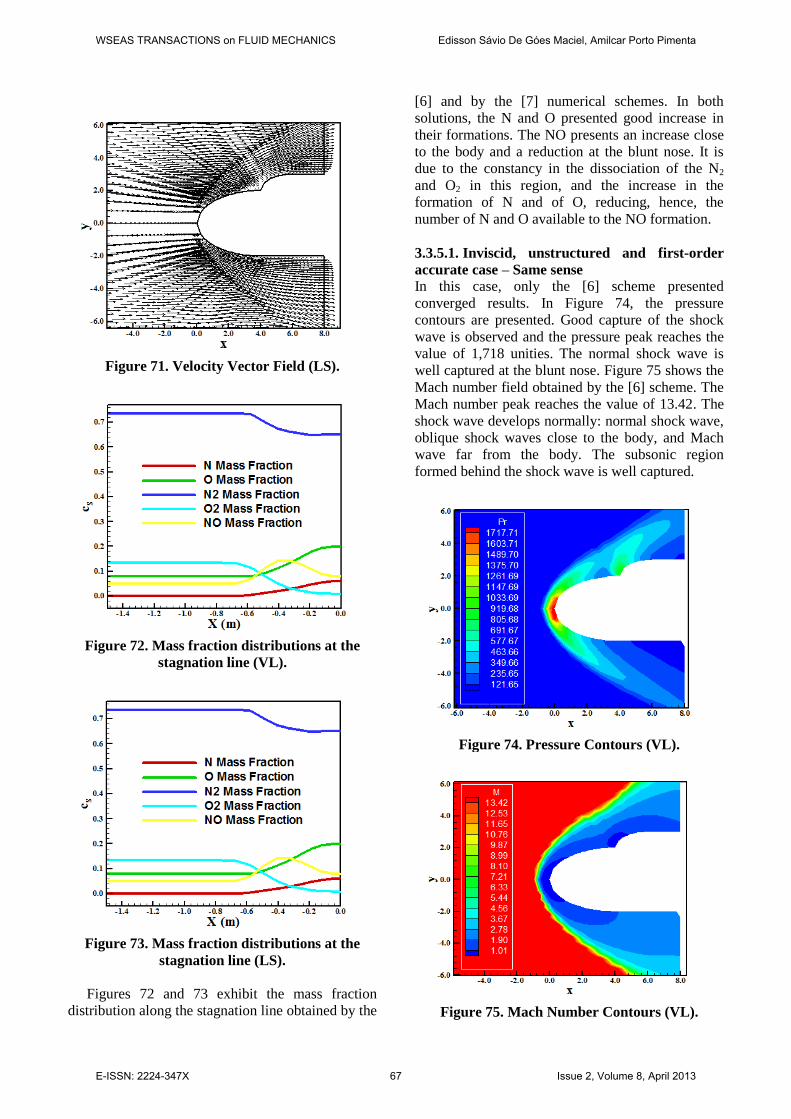
Figure 71. Velocity Vector Field (LS).
Figure 72. Mass fraction distributions at the
stagnation line (VL).
Figure 73. Mass fraction distributions at the
stagnation line (LS).
Figures 72 and 73 exhibit the mass fraction
distribution along the stagnation line obtained by the
[6] and by the [7] numerical schemes. In both
solutions, the N and O presented good increase in
their formations. The NO presents an increase close
to the body and a reduction at the blunt nose. It is
due to the constancy in the dissociation of the N2
and O2 in this region, and the increase in the
formation of N and of O, reducing, hence, the
number of N and O available to the NO formation.
3.3.5.1. Inviscid, unstructured and first-order
accurate case – Same sense
In this case, only the [6] scheme presented
converged results. In Figure 74, the pressure
contours are presented. Good capture of the shock
wave is observed and the pressure peak reaches the
value of 1,718 unities. The normal shock wave is
well captured at the blunt nose. Figure 75 shows the
Mach number field obtained by the [6] scheme. The
Mach number peak reaches the value of 13.42. The
shock wave develops normally: normal shock wave,
oblique shock waves close to the body, and Mach
wave far from the body. The subsonic region
formed behind the shock wave is well captured.
Figure 74. Pressure Contours (VL).
Figure 75. Mach Number Contours (VL).
WSEAS TRANSACTIONS on FLUID MECHANICS Edisson Sávio De Góes Maciel, Amilcar Porto Pimenta
E-ISSN: 2224-347X 67 Issue 2, Volume 8, April 2013
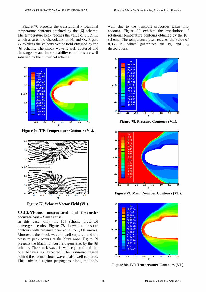
Figure 76 presents the translational / rotational
temperature contours obtained by the [6] scheme.
The temperature peak reaches the value of 8,359 K,
which assures the dissociation of N2 and O2. Figure
77 exhibits the velocity vector field obtained by the
[6] scheme. The shock wave is well captured and
the tangency and impermeability conditions are well
satisfied by the numerical scheme.
Figure 76. T/R Temperature Contours (VL).
Figure 77. Velocity Vector Field (VL).
3.3.5.2. Viscous, unstructured and first-order
accurate case – Same sense
In this case, only the [6] scheme presented
converged results. Figure 78 shows the pressure
contours with pressure peak equal to 1,891 unities.
Moreover, the shock wave is well captured and the
pressure peak occurs at the blunt nose. Figure 79
presents the Mach number field generated by the [6]
scheme. The shock wave is well captured and this
one behaves as expected. The subsonic region
behind the normal shock wave is also well captured.
This subsonic region propagates along the body
wall, due to the transport properties taken into
account. Figure 80 exhibits the translational /
rotational temperature contours obtained by the [6]
scheme. The temperature peak reaches the value of
8,955 K, which guarantees the N2 and O2
dissociations.
Figure 78. Pressure Contours (VL).
Figure 79. Mach Number Contours (VL).
Figure 80. T/R Temperature Contours (VL).
WSEAS TRANSACTIONS on FLUID MECHANICS Edisson Sávio De Góes Maciel, Amilcar Porto Pimenta
E-ISSN: 2224-347X 68 Issue 2, Volume 8, April 2013
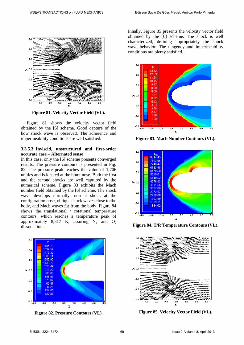
Figure 81. Velocity Vector Field (VL).
Figure 81 shows the velocity vector field
obtained by the [6] scheme. Good capture of the
bow shock wave is observed. The adherence and
impermeability conditions are well satisfied.
3.3.5.3. Inviscid, unstructured and first-order
accurate case – Alternated sense
In this case, only the [6] scheme presents converged
results. The pressure contours is presented in Fig.
82. The pressure peak reaches the value of 1,706
unities and is located at the blunt nose. Both the first
and the second shocks are well captured by the
numerical scheme. Figure 83 exhibits the Mach
number field obtained by the [6] scheme. The shock
wave develops normally: normal shock at the
configuration nose, oblique shock waves close to the
body, and Mach waves far from the body. Figure 84
shows the translational / rotational temperature
contours, which reaches a temperature peak of
approximately 8,317 K, assuring N2 and O2
dissociations.
Figure 82. Pressure Contours (VL).
Finally, Figure 85 presents the velocity vector field
obtained by the [6] scheme. The shock is well
characterized, defining appropriately the shock
wave behavior. The tangency and impermeability
conditions are plenty satisfied.
Figure 83. Mach Number Contours (VL).
Figure 84. T/R Temperature Contours (VL).
Figure 85. Velocity Vector Field (VL).
WSEAS TRANSACTIONS on FLUID MECHANICS Edisson Sávio De Góes Maciel, Amilcar Porto Pimenta
E-ISSN: 2224-347X 69 Issue 2, Volume 8, April 2013
3.3.5.4. Viscous, unstructured and first-order
accurate case – Alternated sense
Both schemes did not present converged results.
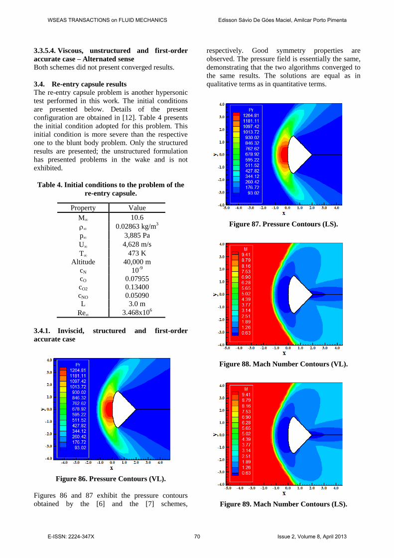
3.4. Re-entry capsule results
The re-entry capsule problem is another hypersonic
test performed in this work. The initial conditions
are presented below. Details of the present
configuration are obtained in [12]. Table 4 presents
the initial condition adopted for this problem. This
initial condition is more severe than the respective
one to the blunt body problem. Only the structured
results are presented; the unstructured formulation
has presented problems in the wake and is not
exhibited.
Table 4. Initial conditions to the problem of the
re-entry capsule.
Property Value
M 10.6
0.02863 kg/m3
p 3,885 Pa
U 4,628 m/s
T 473 K
Altitude 40,000 m
cN 10-9
cO 0.07955
cO2 0.13400
cNO 0.05090
L 3.0 m
Re 3.468x10⁶
3.4.1. Inviscid, structured and first-order
accurate case
Figure 86. Pressure Contours (VL).
Figures 86 and 87 exhibit the pressure contours
obtained by the [6] and the [7] schemes,
respectively. Good symmetry properties are
observed. The pressure field is essentially the same,
demonstrating that the two algorithms converged to
the same results. The solutions are equal as in
qualitative terms as in quantitative terms.
Figure 87. Pressure Contours (LS).
Figure 88. Mach Number Contours (VL).
Figure 89. Mach Number Contours (LS).
WSEAS TRANSACTIONS on FLUID MECHANICS Edisson Sávio De Góes Maciel, Amilcar Porto Pimenta
E-ISSN: 2224-347X 70 Issue 2, Volume 8, April 2013
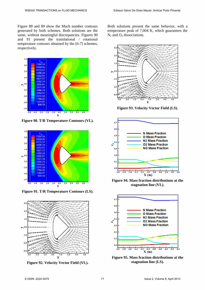
Figure 88 and 89 show the Mach number contours
generated by both schemes. Both solutions are the
same, without meaningful discrepancies. Figures 90
and 91 present the translational / rotational
temperature contours obtained by the [6-7] schemes,
respectively.
Figure 90. T/R Temperature Contours (VL).
Figure 91. T/R Temperature Contours (LS).
Figure 92. Velocity Vector Field (VL).
Both solutions present the same behavior, with a
temperature peak of 7,004 K, which guarantees the
N2 and O2 dissociations.
Figure 93. Velocity Vector Field (LS).
Figure 94. Mass fraction distributions at the
stagnation line (VL).
Figure 95. Mass fraction distributions at the
stagnation line (LS).
WSEAS TRANSACTIONS on FLUID MECHANICS Edisson Sávio De Góes Maciel, Amilcar Porto Pimenta
E-ISSN: 2224-347X 71 Issue 2, Volume 8, April 2013
Figures 92 and 93 exhibit the velocity vector
field obtained by the [6-7] schemes, respectively.
Good symmetry properties are observed. The
impermeability and tangency conditions are well
satisfied by both schemes.
Figures 94 and 95 show the mass fraction
distributions, along the stagnation line of the re-
entry capsule, obtained by the [6] and the [7]
algorithms. Good formation of N and O is observed,
with reasonable formation of NO. The same aspects
observed for NO in other cases are valid herein.
Both solutions are the same, without meaningful
differences.
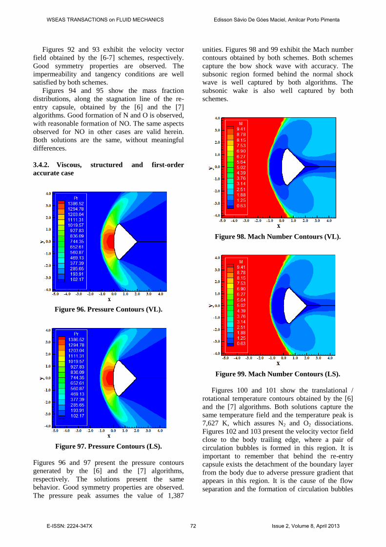
3.4.2. Viscous, structured and first-order
accurate case
Figure 96. Pressure Contours (VL).
Figure 97. Pressure Contours (LS).
Figures 96 and 97 present the pressure contours
generated by the [6] and the [7] algorithms,
respectively. The solutions present the same
behavior. Good symmetry properties are observed.
The pressure peak assumes the value of 1,387
unities. Figures 98 and 99 exhibit the Mach number
contours obtained by both schemes. Both schemes
capture the bow shock wave with accuracy. The
subsonic region formed behind the normal shock
wave is well captured by both algorithms. The
subsonic wake is also well captured by both
schemes.
Figure 98. Mach Number Contours (VL).
Figure 99. Mach Number Contours (LS).
Figures 100 and 101 show the translational /
rotational temperature contours obtained by the [6]
and the [7] algorithms. Both solutions capture the
same temperature field and the temperature peak is
7,627 K, which assures N2 and O2 dissociations.
Figures 102 and 103 present the velocity vector field
close to the body trailing edge, where a pair of
circulation bubbles is formed in this region. It is
important to remember that behind the re-entry
capsule exists the detachment of the boundary layer
from the body due to adverse pressure gradient that
appears in this region. It is the cause of the flow
separation and the formation of circulation bubbles
WSEAS TRANSACTIONS on FLUID MECHANICS Edisson Sávio De Góes Maciel, Amilcar Porto Pimenta
E-ISSN: 2224-347X 72 Issue 2, Volume 8, April 2013
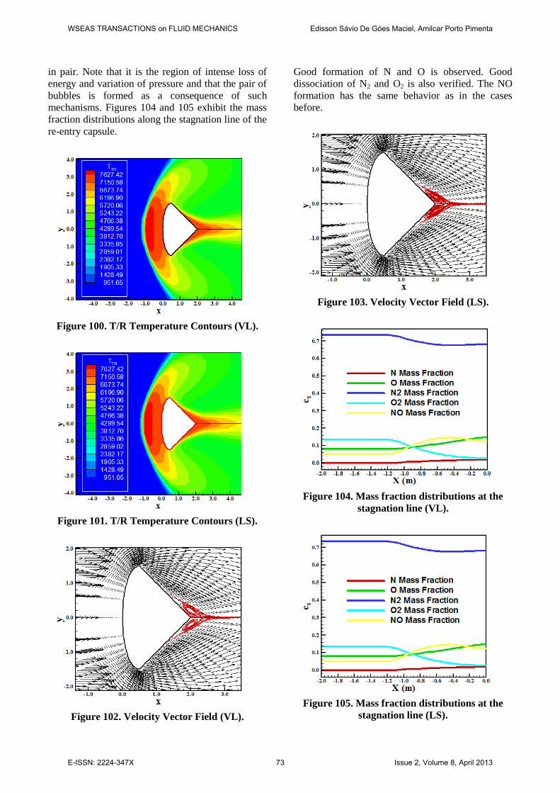
in pair. Note that it is the region of intense loss of
energy and variation of pressure and that the pair of
bubbles is formed as a consequence of such
mechanisms. Figures 104 and 105 exhibit the mass
fraction distributions along the stagnation line of the
re-entry capsule.
Figure 100. T/R Temperature Contours (VL).
Figure 101. T/R Temperature Contours (LS).
Figure 102. Velocity Vector Field (VL).
Good formation of N and O is observed. Good
dissociation of N2 and O2 is also verified. The NO
formation has the same behavior as in the cases
before.
Figure 103. Velocity Vector Field (LS).
Figure 104. Mass fraction distributions at the
stagnation line (VL).
Figure 105. Mass fraction distributions at the
stagnation line (LS).
WSEAS TRANSACTIONS on FLUID MECHANICS Edisson Sávio De Góes Maciel, Amilcar Porto Pimenta
E-ISSN: 2224-347X 73 Issue 2, Volume 8, April 2013

3.4.3. Inviscid, structured and second-order
accurate case
Figure 106. Pressure Contours (VL).
Figure 107. Pressure Contours (LS).
Figure 108. Mach Number Contours (VL).
Figures 106 and 107 show the pressure contours in
the field obtained by the [6] and the [7] schemes,
respectively. The most severe pressure field is
obtained by the [6] scheme, characterizing this one
as more conservative. Good symmetry properties
are observed. The bow shock wave is well captured.
Figure 109. Mach Number Contours (LS).
Figure 110. T/R Temperature Contours (VL).
Figure 111. T/R Temperature Contours (LS).
WSEAS TRANSACTIONS on FLUID MECHANICS Edisson Sávio De Góes Maciel, Amilcar Porto Pimenta
E-ISSN: 2224-347X 74 Issue 2, Volume 8, April 2013
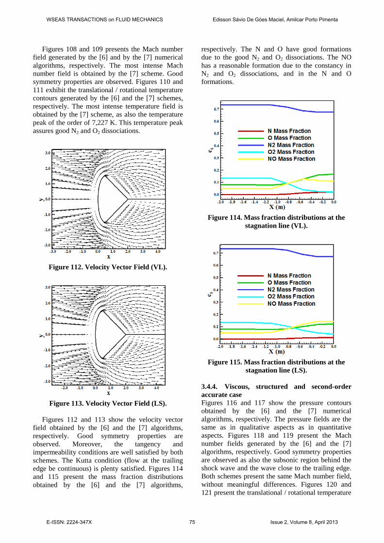
Figures 108 and 109 presents the Mach number
field generated by the [6] and by the [7] numerical
algorithms, respectively. The most intense Mach
number field is obtained by the [7] scheme. Good
symmetry properties are observed. Figures 110 and
111 exhibit the translational / rotational temperature
contours generated by the [6] and the [7] schemes,
respectively. The most intense temperature field is
obtained by the [7] scheme, as also the temperature
peak of the order of 7,227 K. This temperature peak
assures good N2 and O2 dissociations.
Figure 112. Velocity Vector Field (VL).
Figure 113. Velocity Vector Field (LS).
Figures 112 and 113 show the velocity vector
field obtained by the [6] and the [7] algorithms,
respectively. Good symmetry properties are
observed. Moreover, the tangency and
impermeability conditions are well satisfied by both
schemes. The Kutta condition (flow at the trailing
edge be continuous) is plenty satisfied. Figures 114
and 115 present the mass fraction distributions
obtained by the [6] and the [7] algorithms,
respectively. The N and O have good formations
due to the good N2 and O2 dissociations. The NO
has a reasonable formation due to the constancy in
N2 and O2 dissociations, and in the N and O
formations.
Figure 114. Mass fraction distributions at the
stagnation line (VL).
Figure 115. Mass fraction distributions at the
stagnation line (LS).
3.4.4. Viscous, structured and second-order
accurate case Figures 116 and 117 show the pressure contours
obtained by the [6] and the [7] numerical
algorithms, respectively. The pressure fields are the
same as in qualitative aspects as in quantitative
aspects. Figures 118 and 119 present the Mach
number fields generated by the [6] and the [7]
algorithms, respectively. Good symmetry properties
are observed as also the subsonic region behind the
shock wave and the wave close to the trailing edge.
Both schemes present the same Mach number field,
without meaningful differences. Figures 120 and
121 present the translational / rotational temperature
WSEAS TRANSACTIONS on FLUID MECHANICS Edisson Sávio De Góes Maciel, Amilcar Porto Pimenta
E-ISSN: 2224-347X 75 Issue 2, Volume 8, April 2013
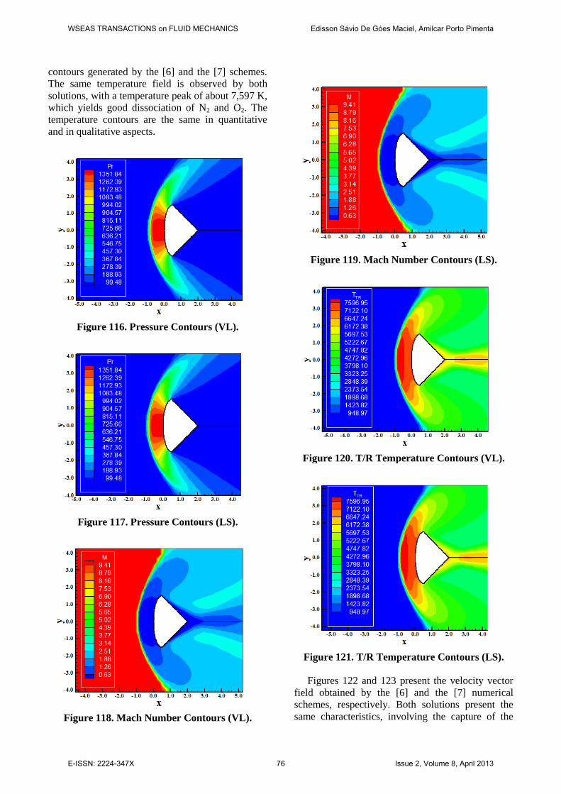
contours generated by the [6] and the [7] schemes.
The same temperature field is observed by both
solutions, with a temperature peak of about 7,597 K,
which yields good dissociation of N2 and O2. The
temperature contours are the same in quantitative
and in qualitative aspects.
Figure 116. Pressure Contours (VL).
Figure 117. Pressure Contours (LS).
Figure 118. Mach Number Contours (VL).
Figure 119. Mach Number Contours (LS).
Figure 120. T/R Temperature Contours (VL).
Figure 121. T/R Temperature Contours (LS).
Figures 122 and 123 present the velocity vector
field obtained by the [6] and the [7] numerical
schemes, respectively. Both solutions present the
same characteristics, involving the capture of the
WSEAS TRANSACTIONS on FLUID MECHANICS Edisson Sávio De Góes Maciel, Amilcar Porto Pimenta
E-ISSN: 2224-347X 76 Issue 2, Volume 8, April 2013
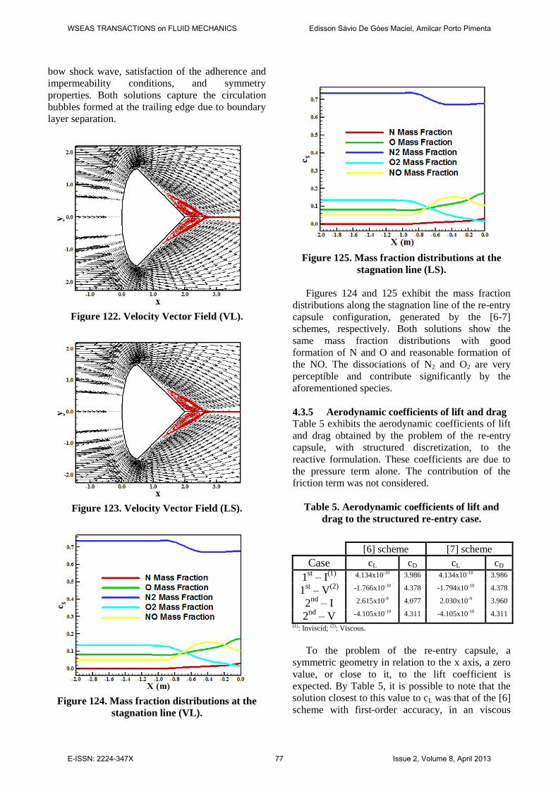
bow shock wave, satisfaction of the adherence and
impermeability conditions, and symmetry
properties. Both solutions capture the circulation
bubbles formed at the trailing edge due to boundary
layer separation.
Figure 122. Velocity Vector Field (VL).
Figure 123. Velocity Vector Field (LS).
Figure 124. Mass fraction distributions at the
stagnation line (VL).
Figure 125. Mass fraction distributions at the
stagnation line (LS).
Figures 124 and 125 exhibit the mass fraction
distributions along the stagnation line of the re-entry
capsule configuration, generated by the [6-7]
schemes, respectively. Both solutions show the
same mass fraction distributions with good
formation of N and O and reasonable formation of
the NO. The dissociations of N2 and O2 are very
perceptible and contribute significantly by the
aforementioned species.
4.3.5 Aerodynamic coefficients of lift and drag
Table 5 exhibits the aerodynamic coefficients of lift
and drag obtained by the problem of the re-entry
capsule, with structured discretization, to the
reactive formulation. These coefficients are due to
the pressure term alone. The contribution of the
friction term was not considered.
Table 5. Aerodynamic coefficients of lift and
drag to the structured re-entry case.
[6] scheme [7] scheme
Case cL cD cL cD
1st – I
(1) 4.134x10⁻¹⁰ 3.986 4.134x10⁻¹⁰ 3.986
1st – V
(2) -1.766x10⁻¹⁰ 4.378 -1.794x10⁻¹⁰ 4.378
2nd
– I 2.615x10⁻⁹ 4.077 2.030x10⁻⁹ 3.960
2nd
– V -4.105x10⁻¹⁰ 4.311 -4.105x10⁻¹⁰ 4.311
(1): Inviscid; (2): Viscous.
To the problem of the re-entry capsule, a
symmetric geometry in relation to the x axis, a zero
value, or close to it, to the lift coefficient is
expected. By Table 5, it is possible to note that the
solution closest to this value to cL was that of the [6]
scheme with first-order accuracy, in an viscous
WSEAS TRANSACTIONS on FLUID MECHANICS Edisson Sávio De Góes Maciel, Amilcar Porto Pimenta
E-ISSN: 2224-347X 77 Issue 2, Volume 8, April 2013
formulation. The maximum cD was obtained by the
solution of the [6] and the [7] schemes, first-order
accurate and employing a viscous formulation.
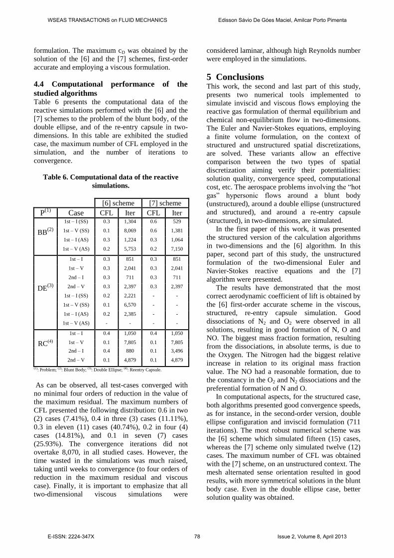
4.4 Computational performance of the
studied algorithms Table 6 presents the computational data of the
reactive simulations performed with the [6] and the
[7] schemes to the problem of the blunt body, of the
double ellipse, and of the re-entry capsule in two-
dimensions. In this table are exhibited the studied
case, the maximum number of CFL employed in the
simulation, and the number of iterations to
convergence.
Table 6. Computational data of the reactive
simulations.
[6] scheme [7] scheme
P(1)
Case CFL Iter CFL Iter
1st – I (SS) 0.3 1,304 0.6 529
BB(2)
1st – V (SS) 0.1 8,069 0.6 1,381
1st – I (AS) 0.3 1,224 0.3 1,064
1st – V (AS) 0.2 5,753 0.2 7,150
1st – I 0.3 851 0.3 851
1st – V 0.3 2,041 0.3 2,041
2nd – I 0.3 711 0.3 711
DE(3)
2nd – V 0.3 2,397 0.3 2,397
1st – I (SS) 0.2 2,221 - -
1st – V (SS) 0.1 6,570 - -
1st – I (AS) 0.2 2,385 - -
1st – V (AS) - - - -
1st – I 0.4 1,050 0.4 1,050
RC(4)
1st – V 0.1 7,805 0.1 7,805
2nd – I 0.4 880 0.1 3,496
2nd – V 0.1 4,879 0.1 4,879
(1): Problem; (2): Blunt Body; (3): Double Ellipse; (4): Reentry Capsule.
As can be observed, all test-cases converged with
no minimal four orders of reduction in the value of
the maximum residual. The maximum numbers of
CFL presented the following distribution: 0.6 in two
(2) cases (7.41%), 0.4 in three (3) cases (11.11%),
0.3 in eleven (11) cases (40.74%), 0.2 in four (4)
cases (14.81%), and 0.1 in seven (7) cases
(25.93%). The convergence iterations did not
overtake 8,070, in all studied cases. However, the
time wasted in the simulations was much raised,
taking until weeks to convergence (to four orders of
reduction in the maximum residual and viscous
case). Finally, it is important to emphasize that all
two-dimensional viscous simulations were
considered laminar, although high Reynolds number
were employed in the simulations.
5 Conclusions This work, the second and last part of this study,
presents two numerical tools implemented to
simulate inviscid and viscous flows employing the
reactive gas formulation of thermal equilibrium and
chemical non-equilibrium flow in two-dimensions.
The Euler and Navier-Stokes equations, employing
a finite volume formulation, on the context of
structured and unstructured spatial discretizations,
are solved. These variants allow an effective
comparison between the two types of spatial
discretization aiming verify their potentialities:
solution quality, convergence speed, computational
cost, etc. The aerospace problems involving the “hot
gas” hypersonic flows around a blunt body
(unstructured), around a double ellipse (unstructured
and structured), and around a re-entry capsule
(structured), in two-dimensions, are simulated. In the first paper of this work, it was presented
the structured version of the calculation algorithms
in two-dimensions and the [6] algorithm. In this
paper, second part of this study, the unstructured
formulation of the two-dimensional Euler and
Navier-Stokes reactive equations and the [7]
algorithm were presented.
The results have demonstrated that the most
correct aerodynamic coefficient of lift is obtained by
the [6] first-order accurate scheme in the viscous,
structured, re-entry capsule simulation. Good
dissociations of N2 and O2 were observed in all
solutions, resulting in good formation of N, O and
NO. The biggest mass fraction formation, resulting
from the dissociations, in absolute terms, is due to
the Oxygen. The Nitrogen had the biggest relative
increase in relation to its original mass fraction
value. The NO had a reasonable formation, due to
the constancy in the O2 and N2 dissociations and the
preferential formation of N and O.
In computational aspects, for the structured case,
both algorithms presented good convergence speeds,
as for instance, in the second-order version, double
ellipse configuration and inviscid formulation (711
iterations). The most robust numerical scheme was
the [6] scheme which simulated fifteen (15) cases,
whereas the [7] scheme only simulated twelve (12)
cases. The maximum number of CFL was obtained
with the [7] scheme, on an unstructured context. The
mesh alternated sense orientation resulted in good
results, with more symmetrical solutions in the blunt
body case. Even in the double ellipse case, better
solution quality was obtained.
WSEAS TRANSACTIONS on FLUID MECHANICS Edisson Sávio De Góes Maciel, Amilcar Porto Pimenta
E-ISSN: 2224-347X 78 Issue 2, Volume 8, April 2013

References:
[1] G. Degrez, and E. Van Der Weide, Upwind
Residual Distribution Schemes for Chemical
Non-Equilibrium Flows, AIAA Paper 99-3366,
1999.
[2] M. Liu, and M. Vinokur, Upwind Algorithms
for General Thermo-Chemical Nonequilibrium
Flows, AIAA Paper 89-0201, 1989.
[3] E. S. G. Maciel, and A. P. Pimenta, Chemical
Non-Equilibrium Reentry Flows in Two-
Dimensions – Part I, submitted to WSEAS
Transactions on Computers (to be published).
[4] E. S. G. Maciel, Analysis of Convergence
Acceleration Techniques Used in Unstructured
Algorithms in the Solution of Aeronautical
Problems – Part I, Proceedings of the XVIII
International Congress of Mechanical
Engineering (XVIII COBEM), Ouro Preto,
MG, Brazil, 2005. [CD-ROM]
[5] E. S. G. Maciel, Analysis of Convergence
Acceleration Techniques Used in Unstructured
Algorithms in the Solution of Aerospace
Problems – Part II, Proceedings of the XII
Brazilian Congress of Thermal Engineering
and Sciences (XII ENCIT), Belo Horizonte,
MG, Brazil, 2008. [CD-ROM]
[6] B. Van Leer, Flux-Vector Splitting for the
Euler Equations, Lecture Notes in Physics,
Springer Verlag, Berlin, Vol. 170, 1982, pp.
507-512.
[7] M. Liou, and C. J. Steffen Jr., A New Flux
Splitting Scheme, Journal of Computational
Physics, Vol. 107, 1993, pp. 23-39.
[8] R. Radespiel, and N. Kroll, Accurate Flux
Vector Splitting for Shocks and Shear Layers,
Journal of Computational Physics, Vol. 121,
1995, pp. 66-78.
[9] L. N. Long, M. M. S. Khan, and H. T. Sharp,
Massively Parallel Three-Dimensional Euler /
Navier-Stokes Method, AIAA Journal, Vol. 29,
No. 5, 1991, pp. 657-666.
[10] R. W. Fox, and A. T. McDonald, Introdução à
Mecânica dos Fluidos, Guanabara, 1988.
[11] E. S. G. Maciel, Relatório ao CNPq (Conselho
Nacional de Desenvolvimento Científico e
Tecnológico) sobre as atividades de pesquisa
realizadas no período de 01/07/2008 até
30/06/2009 com relação ao projeto PDJ número
150143/2008-7, Technical Report, National
Council of Scientific and Technological
Development (CNPq), São José dos Campos,
SP, Brasil, 102p, 2009.
[12] E. S. G. Maciel, and A. P. Pimenta,
Thermochemical Non-Equilibrium Reentry
Flows in Two-Dimensions – Part II, WSEAS
Transactions on Mathematics, Vol. 11, Issue
11, November, 2012, pp. 977-1005.
WSEAS TRANSACTIONS on FLUID MECHANICS Edisson Sávio De Góes Maciel, Amilcar Porto Pimenta
E-ISSN: 2224-347X 79 Issue 2, Volume 8, April 2013