radiation heat-transfer predictions - … · nasa tn d-2867 convective and equilibrium radiation...
TRANSCRIPT
RADIATION HEAT-TRANSFER PREDICTIONS
by P. Cu Zvin Stain buck
Lung ley Reseurch Center ILangley Station, Humpton, Vu.
N A T I O N A L A E R O N A U T I C S A N D SPACE A D M I N I S T R A T I O N W A S H I N G T O N , D. C. J U L Y 1965
https://ntrs.nasa.gov/search.jsp?R=19650017744 2018-08-28T15:32:24+00:00Z
NASA TN D-2867
CONVECTIVE AND EQUILIBRIUM RADIATION HEAT-TRANSFER
PREDICTIONS FOR PROJECT FIRE REENTRY VEHICLE
By P. Calvin Stainback
Langley Research Center Langley Station, Hampton, Va.
NATIONAL AERONAUTICS AND SPACE ADMINISTRATION ~~
For sale by the Clearinghouse for Federal Scientific and Technical Information Springfield, Virginia 22151 - Price $3.00
. 4
CONVECTIVE AND EQUILIBRIUM RADIATION HEAT-TRANSFER
PREDICTIONS FOR PROJECT FIfiE REENTRY VEHICLF:
By P. Calvin Stainback Langley Research Center
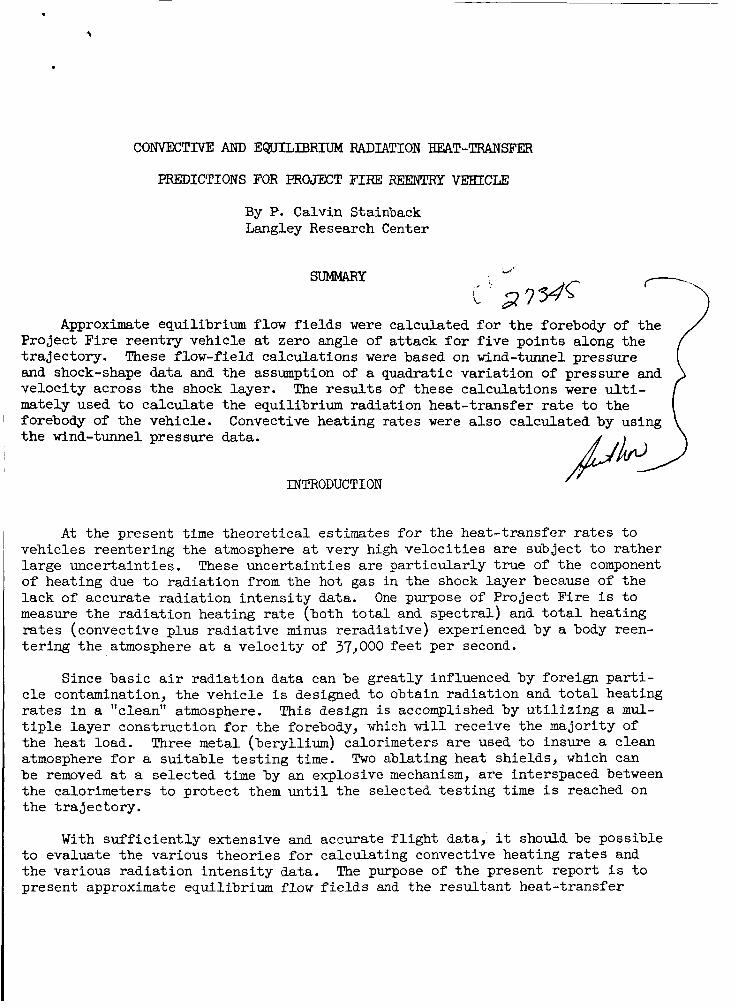
SUMMARY 'J
i ' ; 7 7 9 C Approximate equilibrium flow fields were calculated for the forebody of the
Project Fire reentry vehicle at zero angle of attack for five points along the trajectory. and shock-shape data and the assumption of a quadratic variation of pressure and velocity across the shock layer. mately used to calculate the equilibrium radiation heat-transfer rate to the forebody of the vehicle.
These flow-field calculations were based on wind-tunnel pressure
The results of these calculations were ulti-
Convective heating rates were also calculated by using the wind-tunnel pressure data.
INTRODUCTION
At the present time theoretical estimates for the heat-transfer rates to vehicles reentering the atmosphere at very high velocities are subject to rather large uncertainties. These uncertainties are particularly true of the component of heating due to radiation from the hot gas in the shock layer because of the lack of accurate radiation intensity data. measure the radiation heating rate (both total and spectral) and total heating rates (convective plus radiative minus reradiative) experienced by a body reen- tering the atmosphere at a velocity of 37,000 feet per second.
One purpose of Project Fire is to
Since basic air radiation data can be greatly influenced by foreign parti-
This design is accomplished by utilizing a mul-
Three metal (beryllium) calorimeters are used to insure a clean
cle contamination, the vehicle is designed to obtain radiation and total heating rates in a "clean" atmosphere. tiple layer construction for the forebody, which will receive the majority of the heat load. atmosphere for a suitable testing time. Two ablating heat shields, which can be removed at a selected time by an explosive mechanism, are interspaced between the calorimeters to protect them until the selected testing time is reached on the trajectory.
With sufficiently extensive and accurate flight data, it should be possible to evaluate the various theories for calculating convective heating rates and the various radiation intensity data. present approximate equilibrium flow fields and the resultant heat-transfer
The purpose of the present report is to
calculations for the Project Fire reentry vehicle at several points along its proposed trajectory. The results of these simplified calculations are compared with the results of more exact calculations to determine if the relatively sim- ple analysis can provide heating estimates of usable accuracy.
SYMBOLS
area
constants in eq. (1)
constants in eq. (2)
constants in eq. (2)
drag coefficient
altitude
coordinates of point on body in X,Y,Z coordinate system
specific radiation intensity
mass flow rate into shock layer
mass f l o w rate out of shock layer at 8
normal distance from body surface
number of subdivisions in Simpson's rule
pres sure
stagnation pressure behind normal shock
heat-transfer rate
convective heat-transfer rate
radiative heat-transfer rate
radius
corner radius
ef fec t ive radius
nose spherical radius
cyl indrical radius of body (see f ig . 4)
maximum cyl indrical radius of body
distance between point on body and dV
surface distance from stagnation point
temperature
time (t = o veloci ty
gas cap volume
vehicle weight
body-axis rectangular coordinate system
rectangular coordinate system, origin a t point P on body
reentry angle
l o c a l shock standoff distance f r o m body
at 400,000 f t )
r v o r t i c i t y
e angle measured frm center l i n e of body
' ec angle measured frm forebody-corner l i n e of tangency t o l i n e passing I through any point on corner
angle measured from center l i n e of body t o l i n e passing through point P
i es angle measured from center l i n e of hypothetical sphere
angle measured from center l i n e of body t o forebody-corner l i n e of I
I tangency I eT
densi ty
densi ty at sea l e v e l PSI
3
.-
Velocity, Time, ft/sec
B UI angle measured from body normal to direction of dV
Subscripts :
b at body surface
S behind shock, or of shock
t at stagnation point
W free stream
angle measured from body normal to flow-field velocity
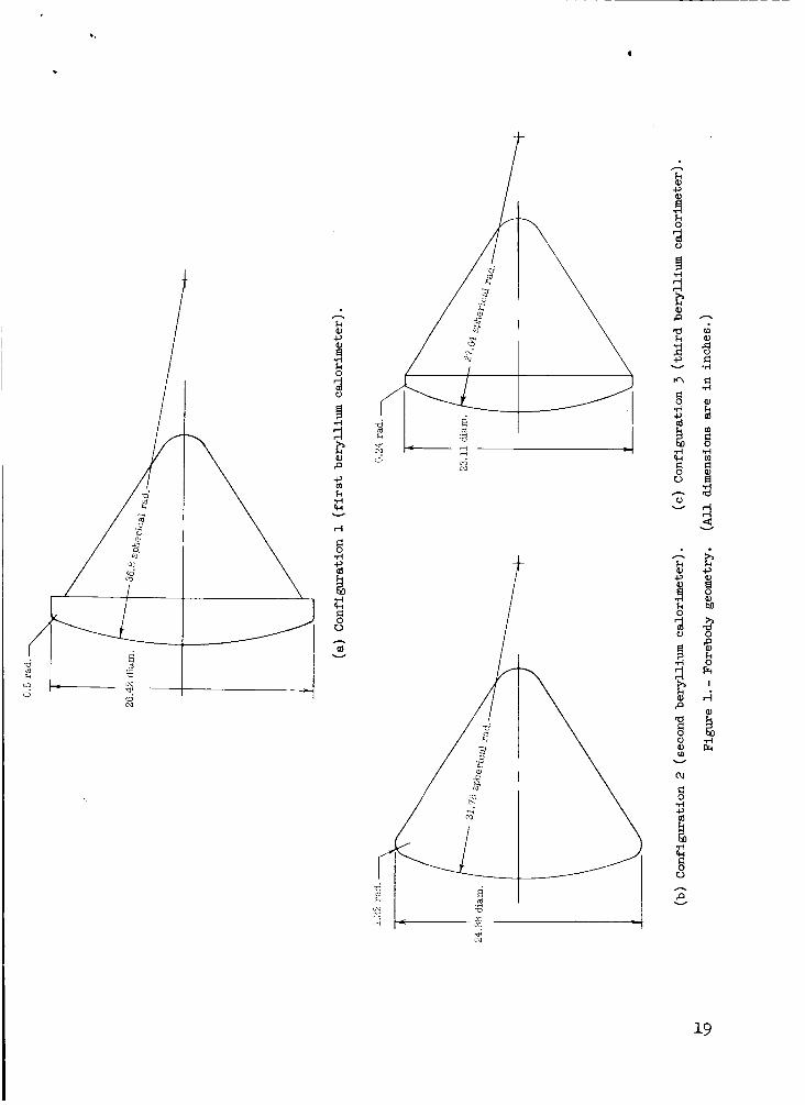
Configuration
FLOW-FIm ANALYSIS
37,058
30, mo 19,500
2:G
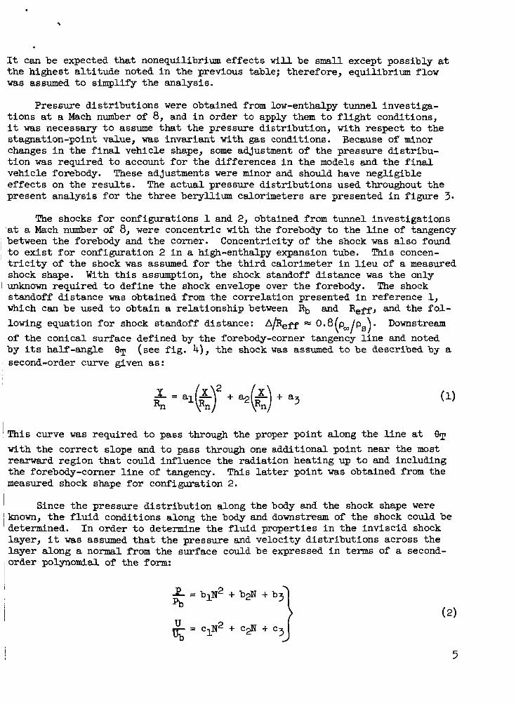
Approximate inviscid flow fields were calculated for the Project Fire reentry vehicle at the following trajectory points, which were taken from the latest trajectory analysis available at the start of the present investigation:
15 1 19 1 25 2 27.6 2 32 3
Altitude,
260,460 218,000 166,000 147,000 120,000
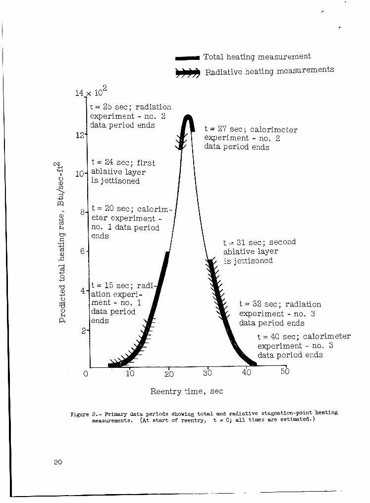
The initial conditions for the trajectory from which the points were taken are: Uw = 37,000 ft/sec; h = 400,000 ft; 7 = -15O; and W/C$ = 35 lb/ft2. The con- figuration numbers represent the shapes of the various beryllium calorimeters which, with the ablation shields, form the forebody of the vehicle. fig. 1.) The altitude and velocity at t = 25 seconds are the approximate con- ditions where the peak total heating rate is expected. A schematic of the heat pulse expected for the vehicle and the periods when the beryllium calorimeter and radiation sensors are expected to obtain useful data are shown in figure 2.
-
(See
The basic assumptions made during the flow-field analysis were:
(1) Equilibrium flow
(2) Pressure distribution known (based on wind-tunnel data)
(3 ) Shock shape known (based on wind-tunnel data)
4
. It can be expected that nonequilibrium effects w i l l be small except possibly a t t h e highest a l t i t ude noted i n the previous table; therefore, equilibrium flow was assumed t o simplify the analysis.
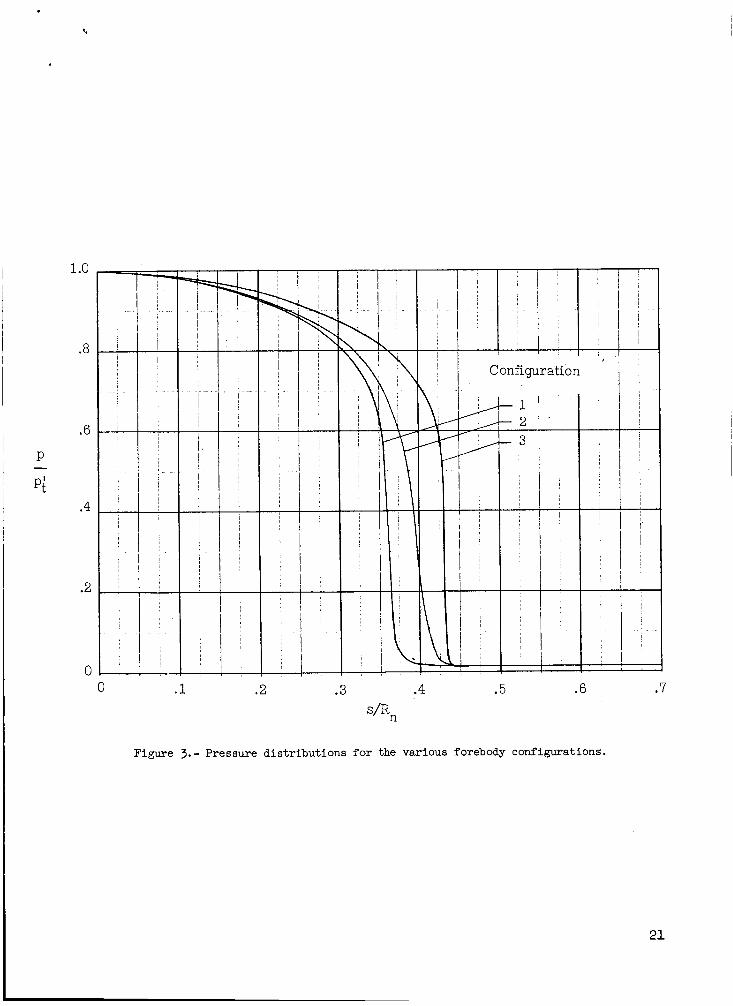
Pressure d is t r ibu t ions were obtained from low-enthalpy tunnel investiga- t ions at a Mach number of 8, and i n order t o apply them t o flight conditions, it was necessary t o assume that the pressure distribution, with respect t o the stawation-point value, w a s invariant with gas conditions. Because of minor changes i n the f inal vehicle shape, some adjustment of the pressure dis t r ibu- t i on w a s required t o account f o r the differences i n the models and the f i n a l vehicle forebody. e f fec ts on the resu l t s . present analysis f o r the three beryllium calorimeters a re presented i n figure 3.
These adjustments were minor and should have negligible The ac tua l pressure dis t r ibut ions used throughout t h e
The shocks f o r configurations 1 and 2, obtained from tunnel investigations
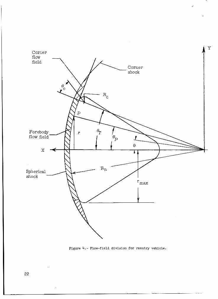
Concentricity of t he shock w a s a l so found at a Mach number of 8, w e r e concentric with the forebody t o the l i n e of tangency between t h e forebody and the corner. t o e x i s t f o r configuration 2 i n a high-enthalpy expansion tube. t r i c i t y of t he shock w a s assumed f o r the t h i r d calorimeter i n l i e u of a measured shock shape. unknown required t o define the shock envelope over t he forebody. standoff distance was obtained from the correlation presented i n reference 1, which can be used t o obtain a relat ionship between F$, and Reff, and the f o l - lowing equation f o r shock standoff distance: A/ReH c 0.8 p p . Downstream
by i ts half-angle 8T second-order curve given as:
"his concen-
With th i s assumption, the shock standoff distance w a s the only "he shock
(a/ .) I of the conical surface defined by the forebody-corner tangency l i n e and noted
(see f i g . 4), the shock was assumed t o be described by a
' ~ h i s curve was required t o pass through the proper point along the l i n e a t 8T with the correct slope and t o pass through one additional point near the most
1 rearward region that could influence the radiation heating up t o and including , t h e forebody-corner l i n e of tangency. This latter point was obtained from the measured shock shape f o r configuration 2.
Since the pressure d is t r ibu t ion along the body and the shock shape were known, t h e f l u i d conditions along the body and downstream of the shock could be determined. I n order t o determine the fluid properties i n t h e inviscid shock layer, it was assumed t h a t t he pressure and velocity d is t r ibu t ions across the layer along a normal from the surface could be expressed i n terms of a second- order polynomial of t h e form:
clN2 + c$ + c3 J U v,=
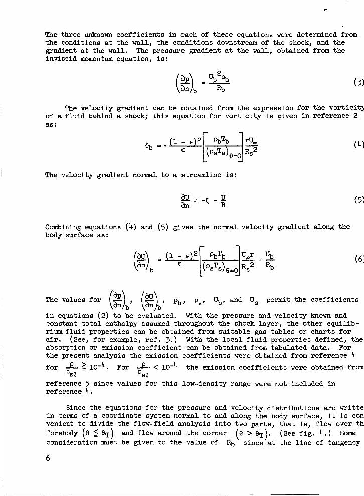
The three unknown coeff ic ients i n each of these equations were determined from the conditions a t the w a l l , the conditions downstream of the shock, and the gradient a t the wall. The pressure gradient at the w a l l , obtained from the inviscid momentum equation, is:
The velocity gradient can be obtained fram the expression f o r the v o r t i c i t j of a f lu id behind a shock; t h i s equation f o r vo r t i c i ty i s given i n reference 2 as :
<b = - (4)
The velocity gradient normal t o a streamline is:
Combining equations (4) and ( 5 ) gives the normal body surface as:
1
veloci ty gradient along the
The values fo r ($$)b, (21, pb, ps, I+,, and Us permit the coefficients
i n equations (2) t o be evaluated. constant t o t a l enthalpy assumed throughout the shock layer, t he other equilib- r i u m f lu id properties can be obtained from su i tab le gas tab les or char ts f o r air. (See, f o r example, ref. 3. ) With the l o c a l f l u i d properties defined, t h e absorption or emission coeff ic ient can be obtained from tabulated data. For t h e present analysis the emission coeff ic ients were obtained from reference 4
With t h e pressure and veloci ty known and
f o r ? - For < loA the emission coefficients were obtained from Psl PSZ
reference 5 since values f o r t h i s low-density range were not included i n reference 4.
Since the equations f o r the pressure and veloci ty d is t r ibu t ions are wr i t t e i n terms of a coordinate system normal t o and along the body surface, it i s con venient t o divide the flow-field analysis i n t o two par ts , t ha t is, flow over t h forebody (e 5 8T) and flow around the corner (See f ig . 4. ) some consideration must be given t o the value of
(e > eT). % since at the l i n e of tangency
6
between the forebody and corner the body radius changes and results in a dis- continuous change in the normal pressure and velocity gradients at Since the flow is subsonic, it does not appear reasonable from a physical view- point to have this discontinuity. continuity in the gradients normal to the body, an effective body radius was calculated. This calculation was made by assuming that the effective radius of the body is equal to the radius of a sphere which has the same pressure gradi- ent along its surface at equal angles with respect to the free-stream velocity. A Newtonian pressure distribution was assumed t o exist over the hypothetical sphere. With these assumptions, the effective body radius becomes:
8 = eT.
Therefore, in order to eliminate this dis-
d P Pt d( s/R)
where
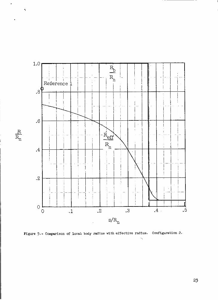
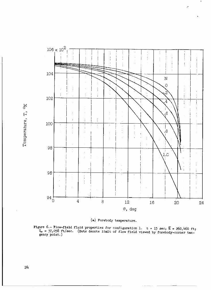
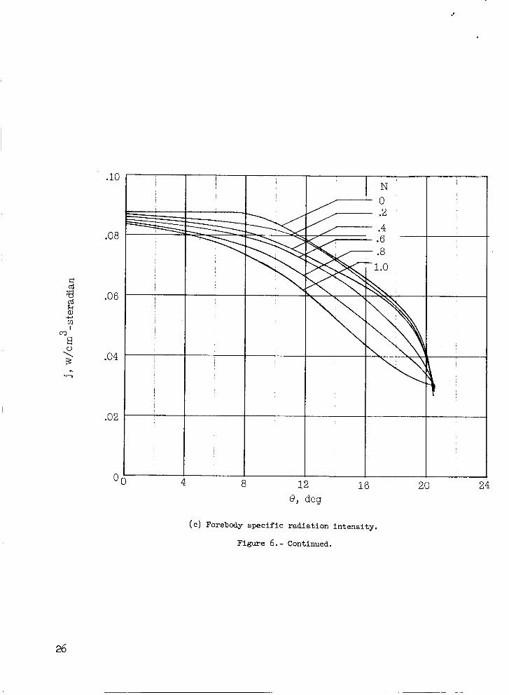
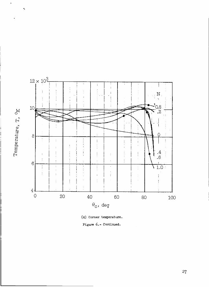
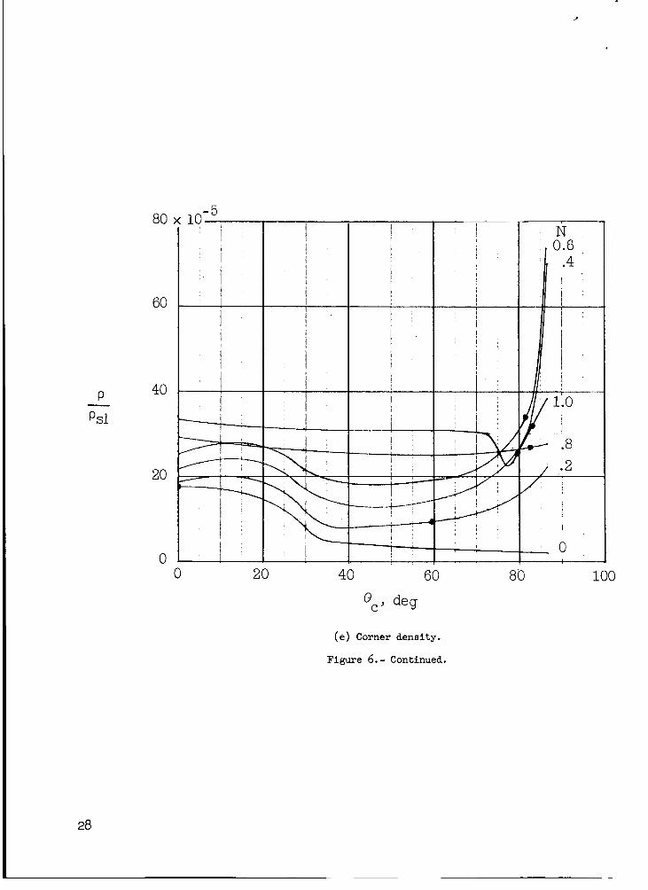
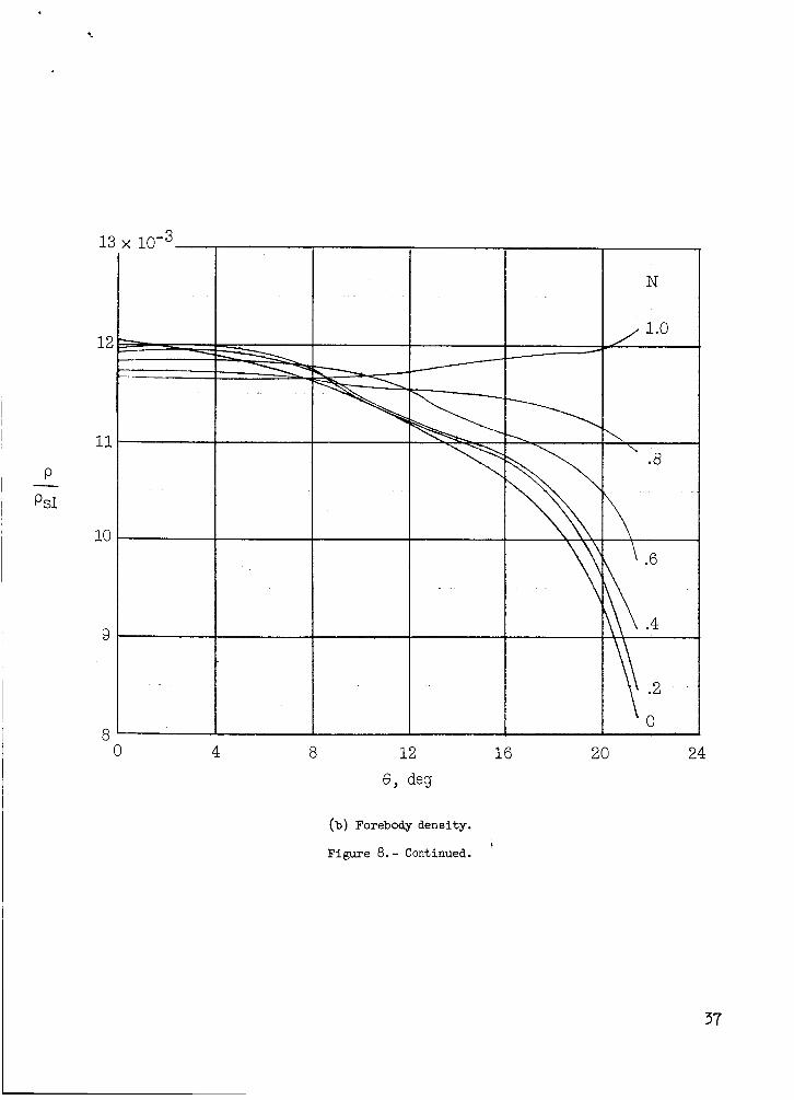
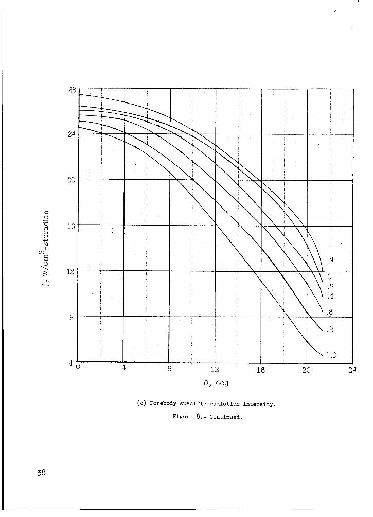
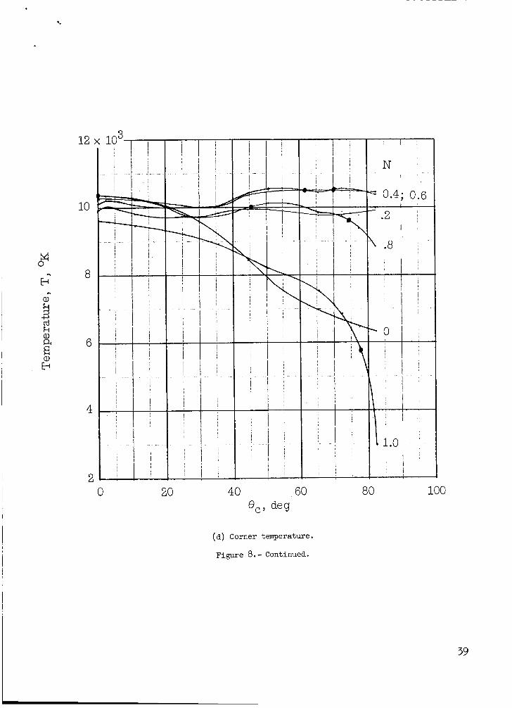
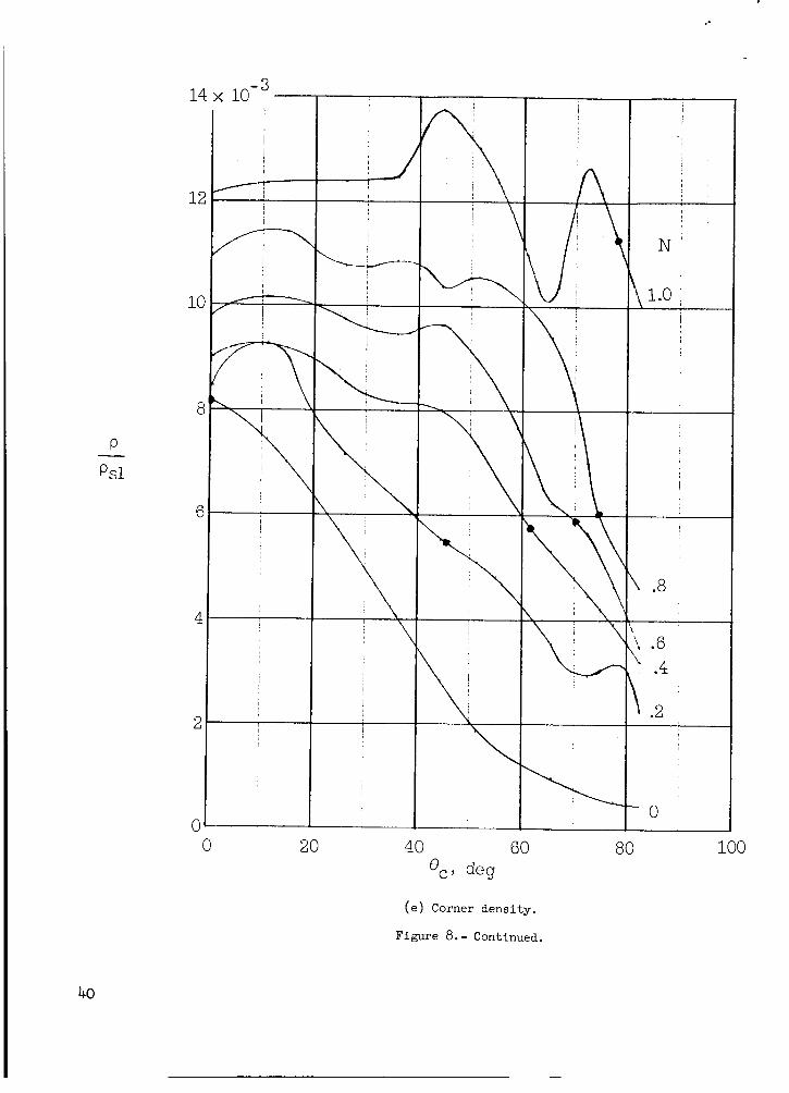
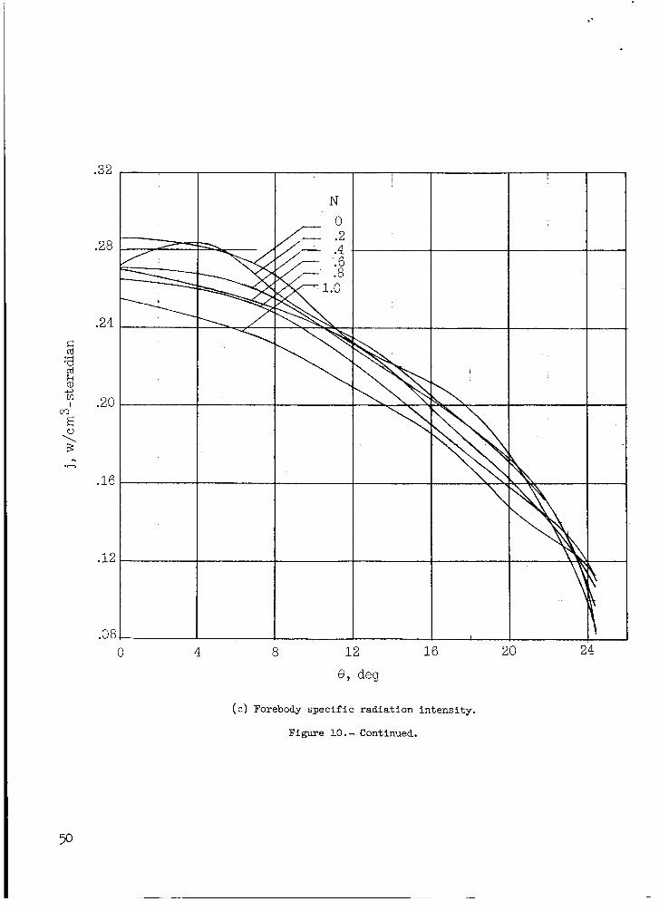
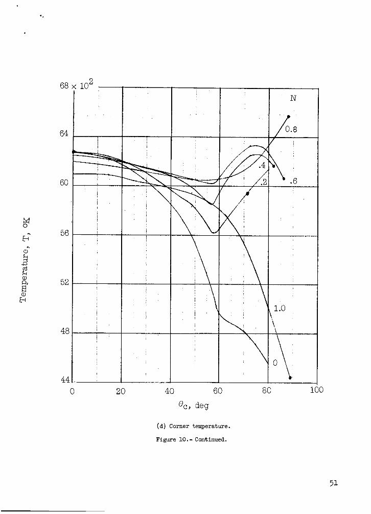
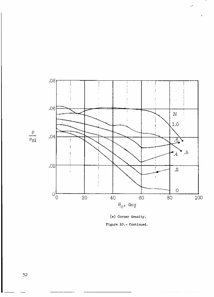
This effective radius was used throughout the analysis for in equations (3) and (6). It should be noted that this definition of Reff should give the same values for Reff at the stagnation point as given in reference 1. A plot of Reff and Rb for configuration 2 is given in figure 5 to show the difference in the two quantities. Figures 6 to 10 present the temperature, density, and specific radiation intensity calculated by the previously discussed method for both the forebody and corner flow fields. vary fairly uniformly over the forebody and around the corner up to a value of 8c of about so to 400. For larger values of 8, the flow-field properties
1 appear to be somewhat erratic, and this can probably be attributed to the sim- 1 plicity of the present method.
is determined from the measured pressure data for the body.
Rb
In general., the fluid properties
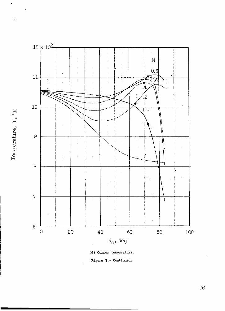
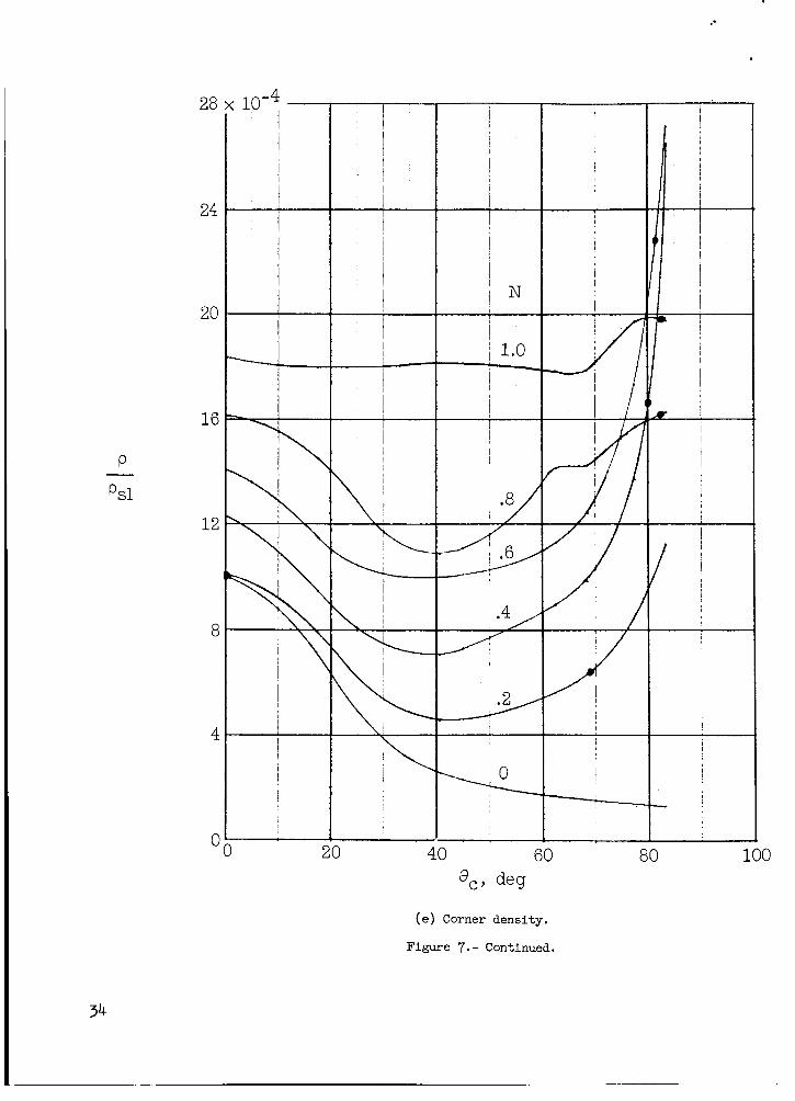
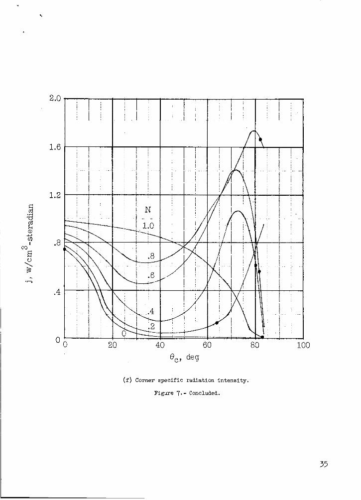
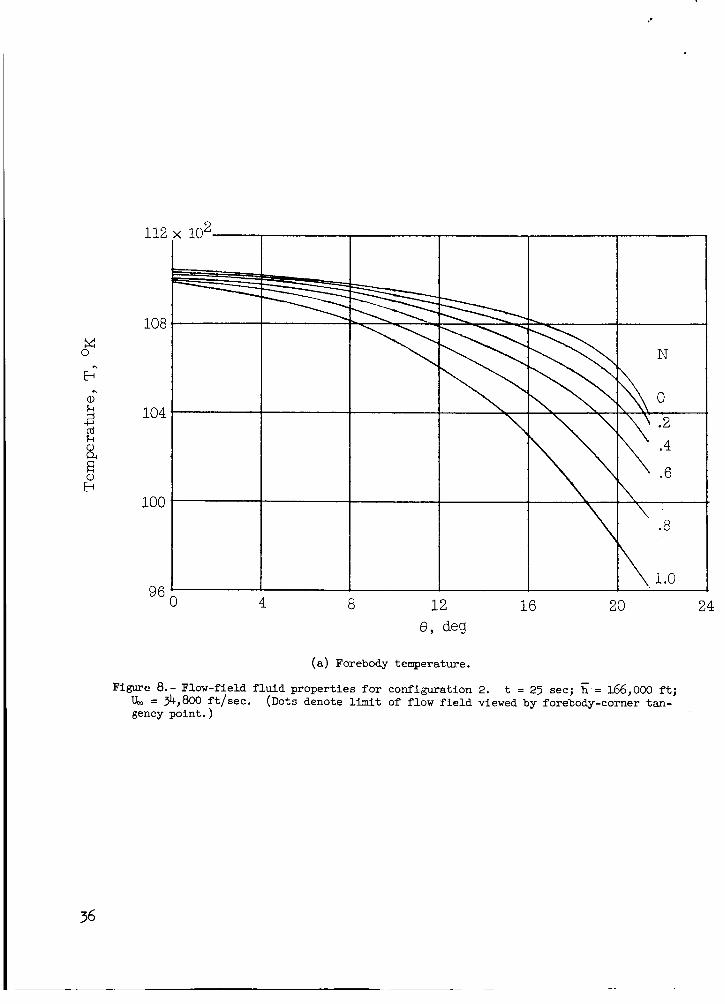
Except for the gas in the immediate vicinity of the point for which the radiation heating rate is being calculated, the irregularity of the flow-field fluid properties for large values of 8, has little influence on the radiation heating rate to the forebody due to the distances and view angle involved. The limit of the flow field that is viewed by the forebody-corner tangency point is noted on the curves in figures 6 to 10 by the dots.
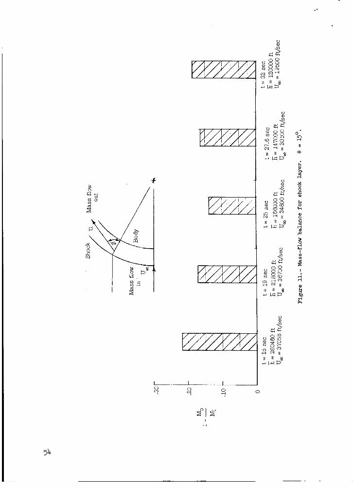
It should be pointed out that although no iterations were made during this analysis, the method employed could be revised to permit iteration on the shock location by balancing the mass flow within the shock layer. In order to obtain some quantitative evaluation of the self consistency of the calculated flow fields, a mass-flow balance was made at are shown in figure It. and indicate that based on the criterion of mass flow, the flow fields appear to be only fairly accurate.
0 = 15O. The results of this balance
The mass-flow balance could be influenced by three things: the calculated density and velocity distributions across the shock layer, the shock standoff distance, and the flow angularity with respect to the area over which the mass- flow balance was calculated. The variation of the flow angle with respect to the normal from the body surface was assumedto be linear between the value at
7
the body (6 = 90°) and the value calculated behind the shock for an oblique shock. the value of Reff* A comparison between the mass-flow balance for R = Reff and R = Rn
between the two methods. The mass-flow balance parameter (1 - 2) for the flow field calculated for R = Reff was 0.132 and for R = R, was 0.1435. Therefore, if the flow-angularity assumption is reasonable, the mass-flow deficit must be predominately due to the shock standoff distance which is too small.
The density and velocity distributions across the shock layer depend on
in equations (3) and (6) indicates that there is little difference
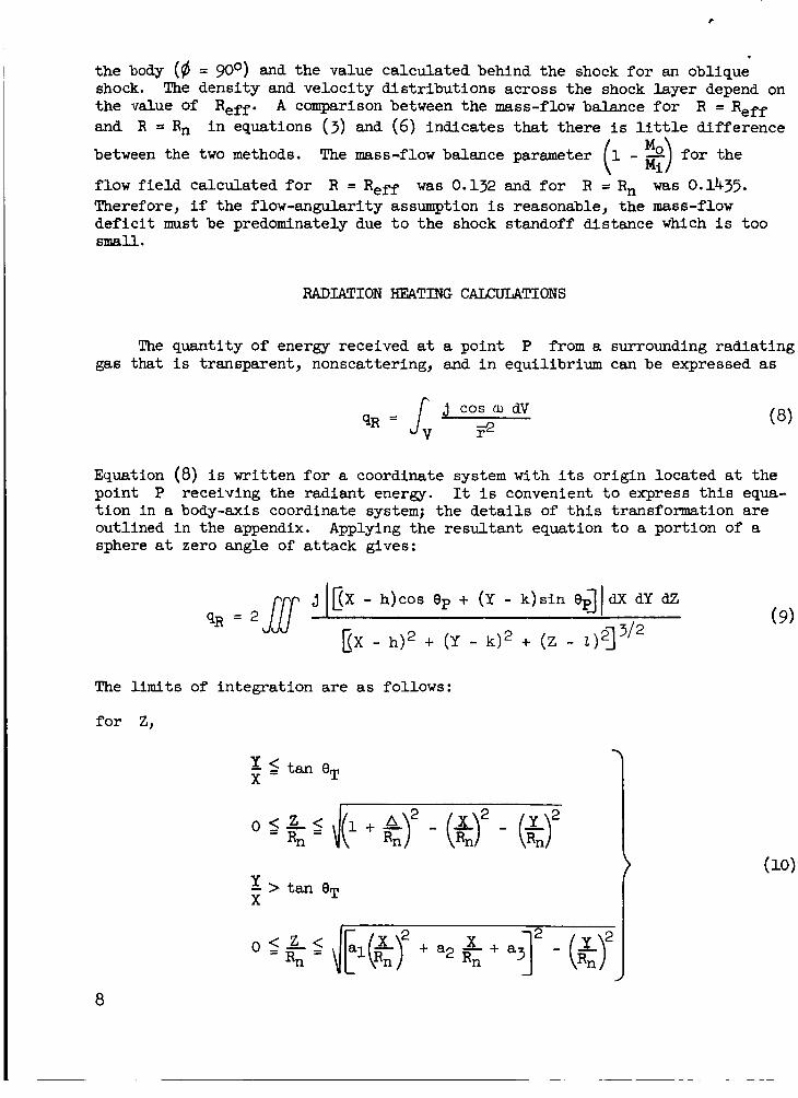
RADIATION HEATING CALCULATIONS
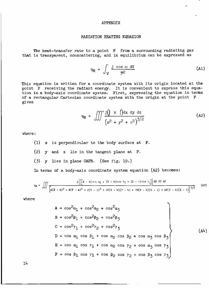
The quantity of energy received at a point P from a surrounding radiating gas that is transparent, nonscattering, and in equilibrium can be expressed as
j cos (u dV ..=s, g
Equation (8) is written for a coordinate system with its origin located at the point P receiving the radiant energy. It is convenient to express this equa- tion in a body-axis coordinate system; the details of this transformation are outlined in the appendix. sphere at zero angle of attack gives:
Applying the resultant equation to a portion of a
j I B X - h)cos ep + (Y - k)sin eP)(dx dy d~
EX - h)* + (Y - k)2 + (Z - 1.1 '3 3'2
The limits of integration are as follows:
for Z,
X X I t an eT
a
( 9 )
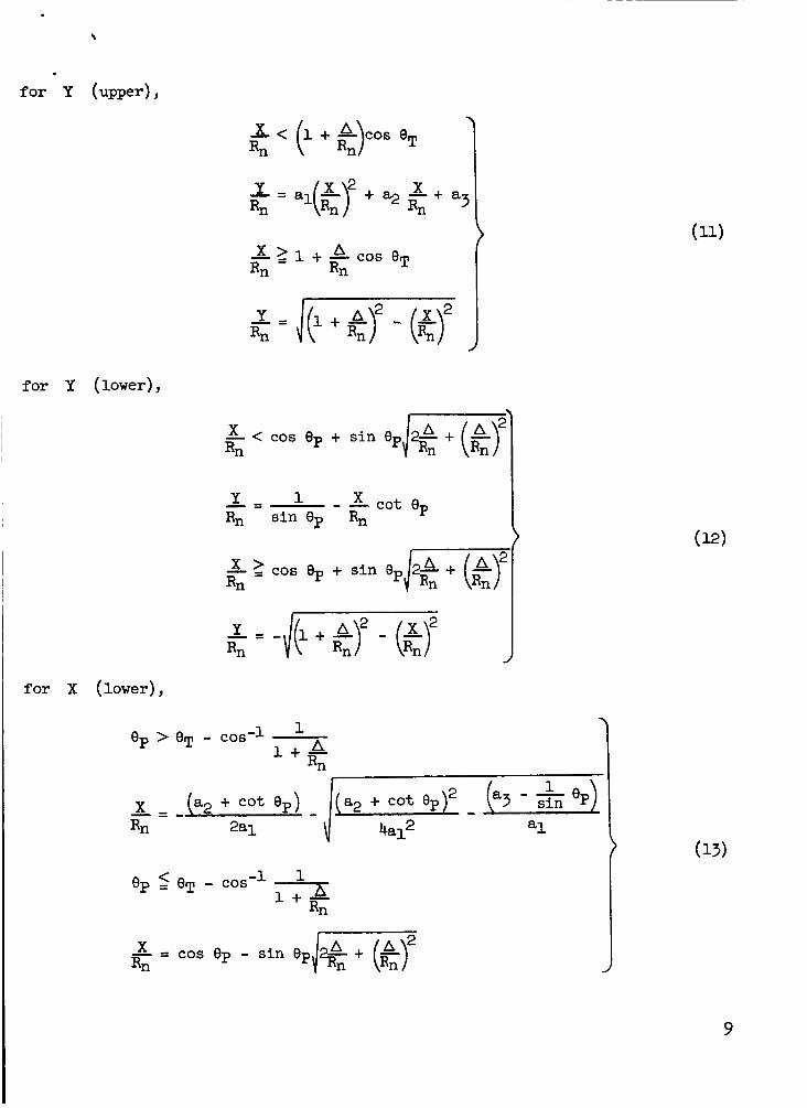
f o r Y (upper),
for Y (lower),
X - C cos eP + s i n 8 Rn
1 X Y Rn s i n 8p Rn
- - cot ep - =
f o r x (lower),
9
t
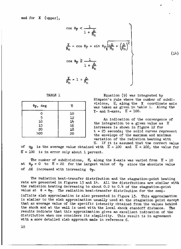
and for X (upper),
1 A 1 + -
cos ep < Rn
1 A 1 + -
cos ep 2 Rn
l!ABm 1
l2 I 5 I 10 I 14 15 16
J Equation ( 9 ) was integrated by
Simpson's rule where the nuniber of subdi- visions, n, along the X coordinate axis was taken as given in table 1. Along the Y- and Z-axes,
- - n = 100.
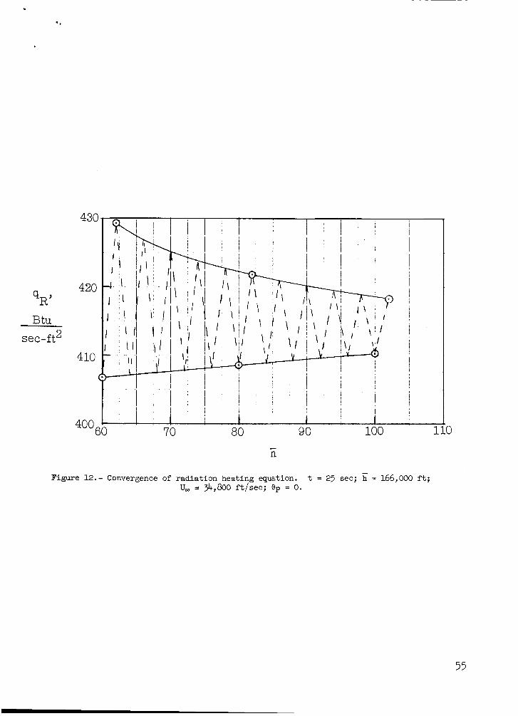
An indication of the convergence of the integration to a given value as increases is shown in figure 12 for t = 25 seconds; the solid curves represent the envelope of the maximum and minimum variation of the radiation heating with Z. If it is assumed that the correct value
E
of qR is the average value obtained with n = 100 and = 102, the value for ff = 100 is in error only about 1 percent.
The number of subdivisions, ii, along the X-axis was varied from = 10 at eP = 0 to T i = 20 for the largest value of 9p since the absolute value of AX increased with increasing 9 ~ .
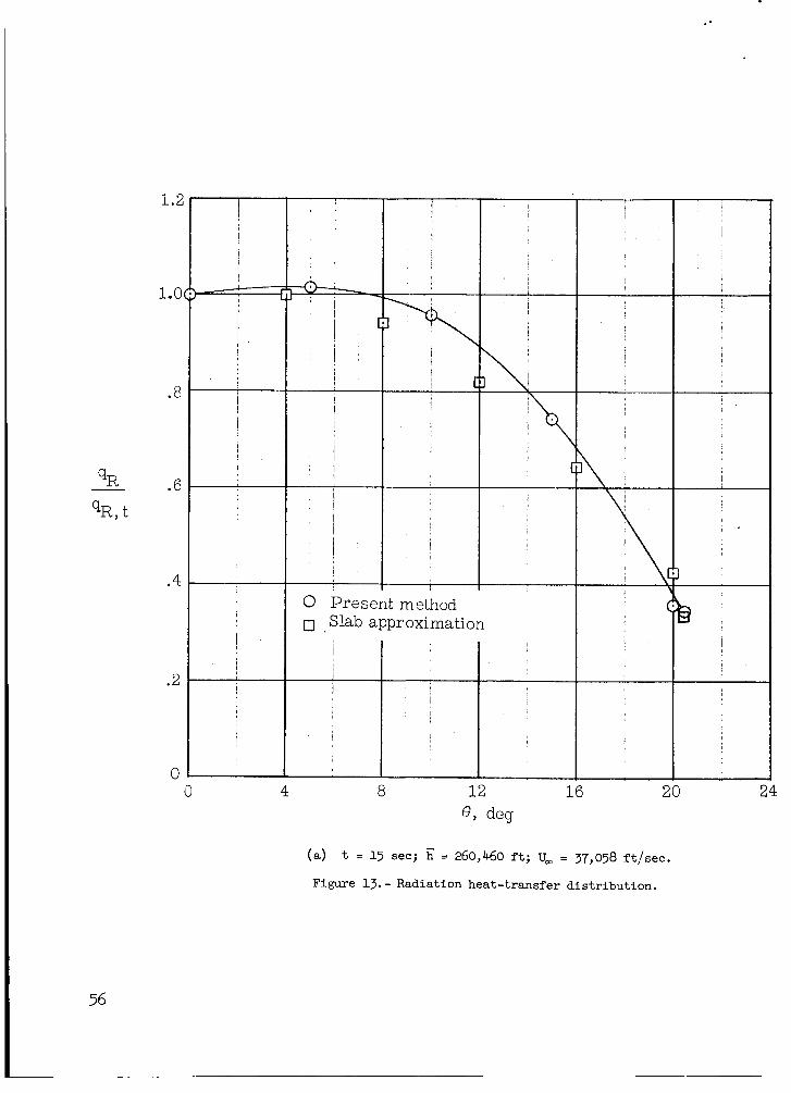
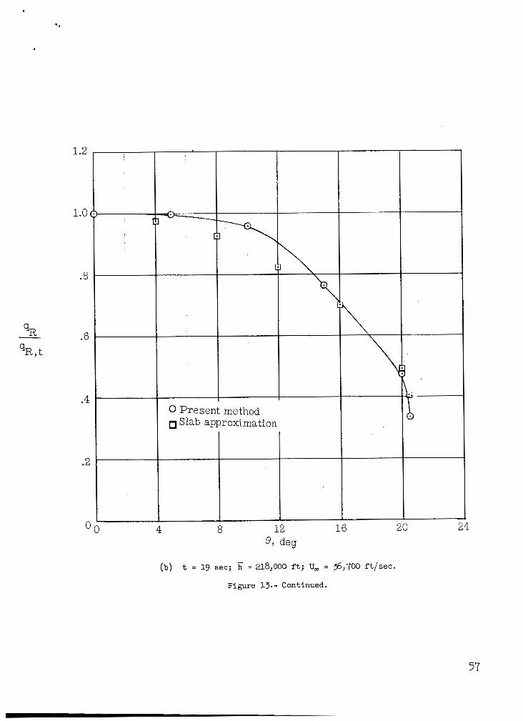
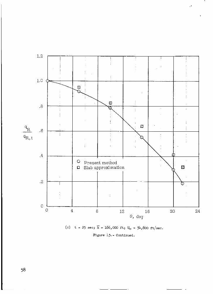
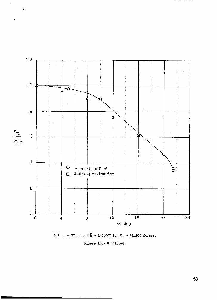
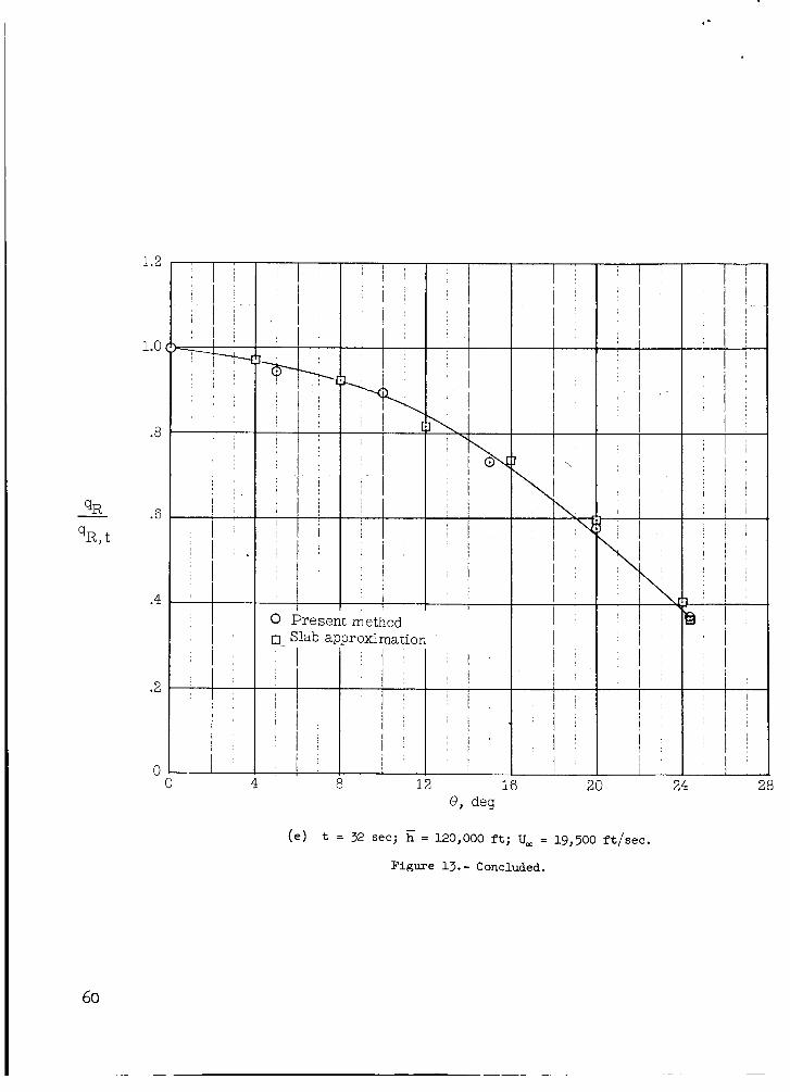
The radiation heat-transfer distribution and the stagnation-point heating rate are presented in figures 13 and 14. the radiation heating decreasing to about 0.2 to 0.4 of the stagnation-point value at 8 = 8T. infinite slab approximation is also presented in figure 13. This approximation is similar to the slab approximation usually used at the stagnation point except that an average value of the specific intensity obtained from the values behind the shock and at the wall is used with the local shock standoff distance. results indicate that this approximation gives an excellent indication of the distribution when one considers its simplicity. with a more detailed slab approach made in reference 6.
All the distributions are similar with
The radiation heat-transfer distribution for the semi-
The
This result is in agreement
10
The mass-flow discrepancy noted previously i n t h e section en t i t l ed "Flow- Field Analysis" w i l l influence the magnitude of the radiation heating since the e r ror i s believed t o be predominantly due t o the shock standoff distance being too small by approximately the same percentage as the mass-flow balance. slab approximation i s considered, the absolute magnitude of the heating would increase i n proportion t o the mass-flow error, but the dis t r ibut ion would be essent ia l ly unchanged.
If the
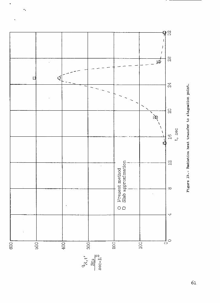
The stagnation-point radiat ive heating rates shown i n figure 14 are rela- t i ve ly low f o r a l l points investigated except f o r t = 25 seconds where the heating r a t e i s about 400 Btu/sec-ft2. approximation f o r the stagnation-point heating r a t e .
Also shown i n figure 14 i s the slab
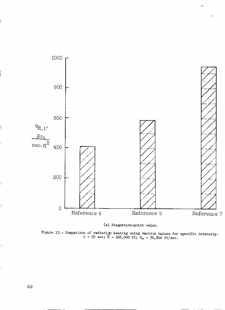
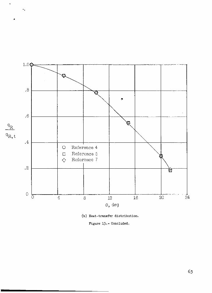
It should be noted tha t the radiative heating r a t e i s dependent on the specific-radiation-intensity data used. To date t h i s gas property i s not known t o great accuracy and different values are given by different investigators. For the most par t the radiation in tens i ty data used f o r t h i s investigation were taken from reference 4 since it w a s generally accepted tha t the best data avai l - able at the start of t h i s investigation are given i n t h i s reference. it has been suggested tha t these in t ens i t i e s are low. I n order t o show the influence of the various radiation in tens i ty data, the stagnation-point heating r a t e and the forebody dis t r ibut ion f o r using the data of references 4, 5, and 7. are presented i n f igure 15. The stagnation-point heat-transfer rates range from 410 Btu/sec-ftZ, i f the data of reference 4 are used, t o 946 Btu/sec-ftZ, f o r the data from reference 7. dis t r ibut ion obtained by using the various specific-intensity data.
Recently
t = 25 seconds were calculated by The re su l t s of these calculations
There w a s no change i n the radiation heating
The difference between the heating estimates can be par t ly a t t r ibu ted t o the larger wavelength range considered f o r calculating the specific i n t ens i t i e s i n reference 7. The wavelength range f o r the data of reference 7 w a s f r o m 0.05 t o 10 microns whereas the range w a s from 0.16 t o 10 microns f o r reference 4. It i s expected that the Project F i r e f l i g h t data w i l l reduce the uncertainty i n predicting the radiat ion heating. It should be noted, however, t ha t most of the added energy i n the wave length increment from 0.05 t o 0.16 micron con- sidered i n reference 7 w i l l not be transmitted t o the vehicle radiation sensors since the quartz windows i n the forebody absorb most of the radiation below about 0.18 micron. way, inferred from convective-heating calculations and measured t o t a l heating ra tes .
Thus, t h i s increment i n radiation heating must be, i n some
I n addition t o t h i s complication, self absorption of radiant energy within the gas cap might become significant, par t icular ly i n the small wavelength region considered i n reference 7.
CONVECTIVE €EATING
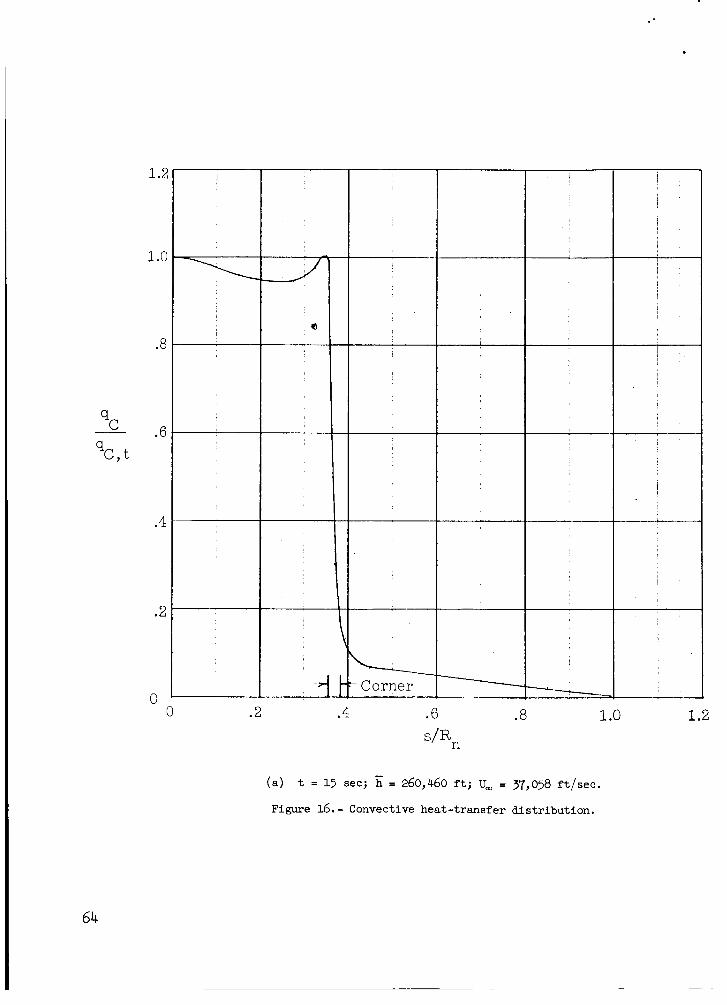
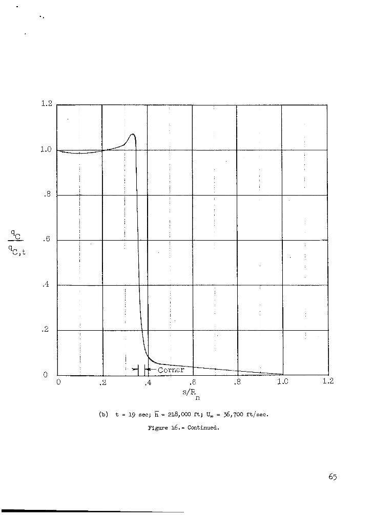
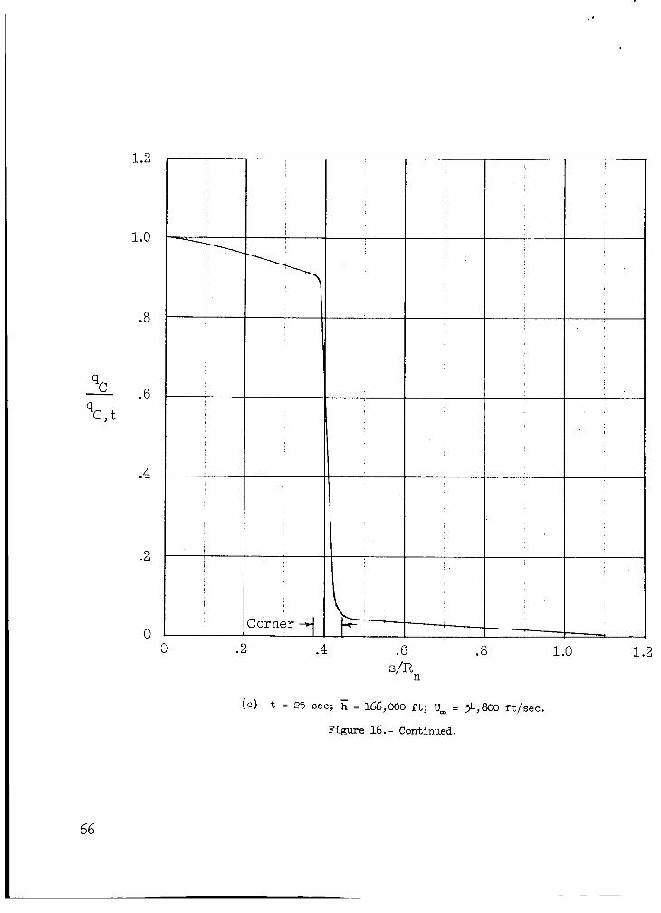
The convective heat-transfer distribution around the vehicle was calcu- la ted by using the correlations presented i n reference 8. calculations of the heat-transfer distribution a re presented i n figure 16.
The results of the
11
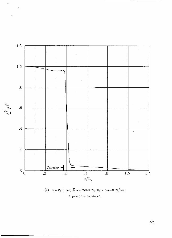
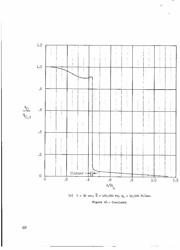
This figure shows that body; the high heating bodies does not occur.
the heating rate i s essent ia l ly constant over the fore- rate sometimes encountered a t the outer edge of blunt The var ia t ion at the outer edge of the body i s never
greater than fL.0 percent of t he stagnation-point value.
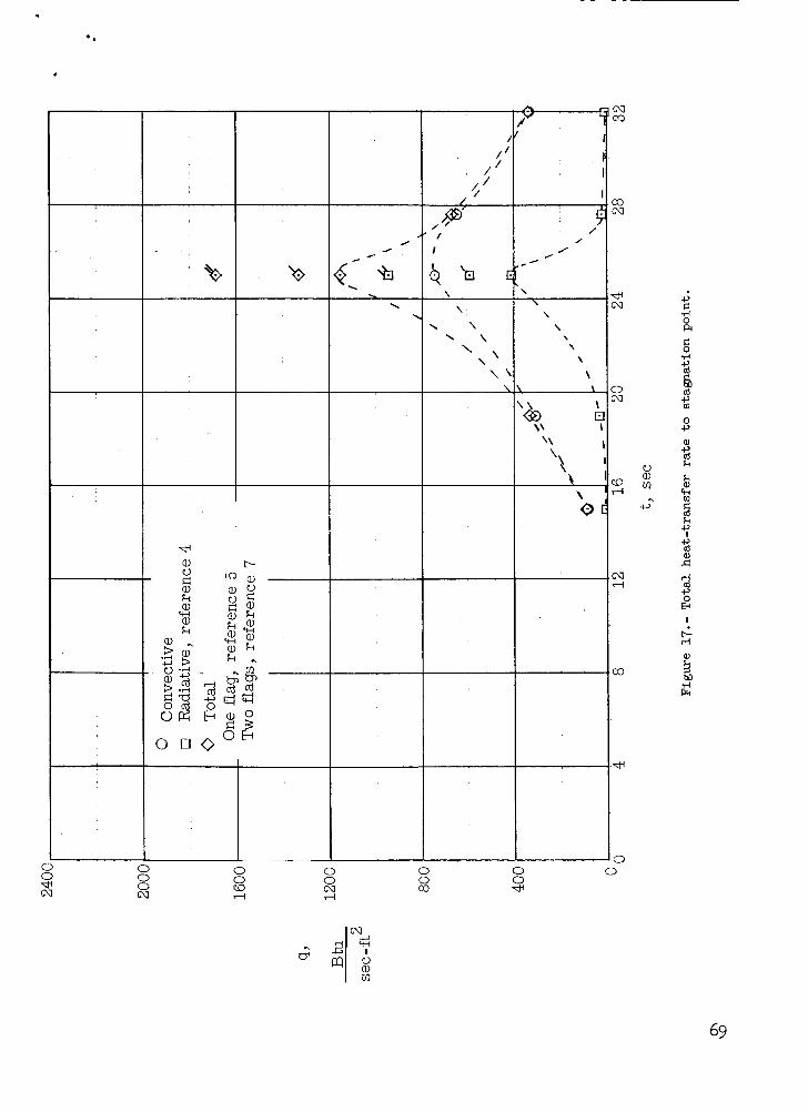
The stagnation-point heat-transfer rate w a s calculated from the correlated The r e s u l t s of these calcu- resu l t s of reference 9 f o r the high-enthalpy case.
l a t ions a re presented i n figure 17. heating rate calculated w a s 740 Btu/sec-ft2. This convective heating rate i s almost twice the radiat ive heating r a t e calculated by the data of reference 4 and about 20 percent l e s s than the rad ia t ive heating rate calculated by the data of reference 7. Thus, it i s not c lear whether the convective heating rate w i l l dominate the peak stagnation-point heating t o the vehicle o r whether radi- a t ive and convective heating w i l l contribute equally t o the t o t a l peak heating rate. The maximum t o t a l heating rate t o the stagnation point w i l l range from about ll50 t o about 1690 Btu/sec-ft2 depending upon the radiat ion data used.
The maximum convective stagnation-point
The radiat ive and t o t a l heating rates are a l so p lo t ted i n figure 17.
COMPARISON OF PRESENT RESULTS WITH MORE EXACT ANALYSES
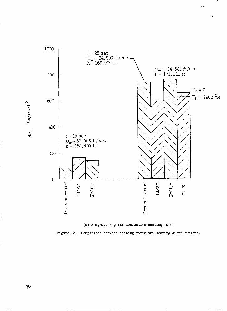
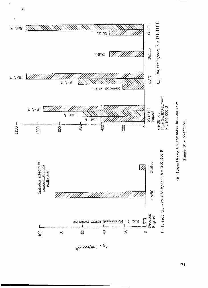
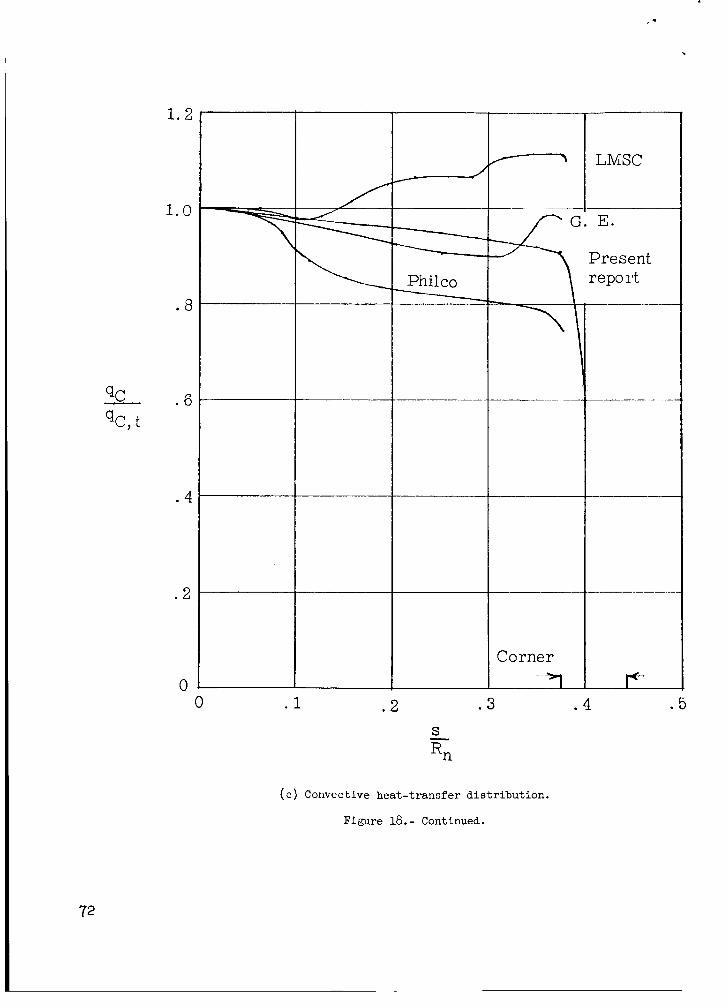
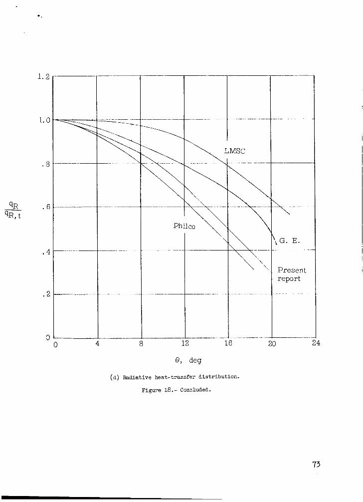
The present r e su l t s are compared with the results of more exact calcula- t i ons made by the General Elec t r ic Company, Lockheed Missiles and Space Company, and Philco Corporation under contract t o the NASA Office of Advanced Research and Technology. ure 18. The f igure indicates that there i s considerable disagreement between the four s e t s of resu l t s . radiative heat-transfer d i s t r ibu t ions and fo r t he stagnation-point radiat ive heating rate except when the same specif ic radiat ion in tens i ty data are used.
The results of these comparisons are shown i n f ig-
This i s par t icu lar ly t rue f o r the convective and
The stagnation-point convective heat-transfer rate of the present report compares favorably w i t h the contractor results except f o r the present results a re about 50 percent of the highest estimate. estimates of t h e stagnation-point radiat ive heating r a t e f o r agree well w i t h the other results provided the same specif ic radiat ion in tens i ty data are used. "here i s a great dea l of difference between the stagnation-point radiative heating r a t e f o r t = 15 seconds where nonequilibrium e f fec t s can influence the radiat ive heating rate. f a i r agreement w i t h Phi lco 's resu l t s .
t = 15 seconds where
t = 25 seconds The present
The present results f o r t h i s case are i n
It is somewhat surprising tha t t h e convective and radiat ion estimates of heat-transfer dis t r ibut ions d i f f e r by such a large amount. The present results f a l l between the maximum and minimum values predicted by the contractors. present radiat ion d is t r ibu t ion agrees c losely with Philco's results whereas the present convective d is t r ibu t ion agrees f a i r l y w e l l w i t h General E lec t r i c ' s resul ts . From an overa l l point of view, the simplified analysis of t he present report gives r e su l t s which compare favorably with the results obtained from more exact calculations.
The
., CONCLUSIONS
Calculations of the approximate equilibrium flow fields for the forebody of the Project Fire reentry vehicle at zero angle of attack and the resulting convective and equilibrium radiation heat-transfer calculations permit the fol- lowing conclusions:
1. The radiation stagnation-point heating rate is greatly influenced by the specific-radiation-intensity data used and ranged from a low of 410 Btu/sec-ftz to a high of 946 Btu/sec-ft2.
2. The radiation heat-transfer rate over the forebody decreases fairly rapidly from the stagnation point to the outer diameter of the vehicle. heating rate at the forebody-corner tangency point is only about 0.2 to 0.4 of the stagnation-point value.
3. The peak convective stagnation-point heating rate is about 740 Btu/sec-ftZ. in a peak total heating rate that ranges from 1150 to 1690 Btu/sec-ft2 depending on the radiation data used.
The
This rate combined with the peak radiation heating results
4. The convective heat-transfer rate over the forebody is essentially con- stant, never varying more than f10 percent of the stagnation-point value.
5. For the case considered, the radiative heat-transfer distributions obtained by a simple slab approximation are in good agreement with those obtained by integrating the specific intensity over the calculated gas cap volume.
6. In general, the simplified analysis of the present report gives results which compare favorably with the results obtained from more exact calculations.
Langley Research Center, National Aeronautics and Space Administration,
Langley Station, Hapton, Va., October 21, 1964.
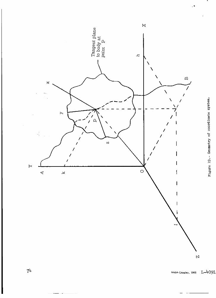
APPENDIX
RADIATION HEATING EQUATION
The heak-transfer rate to a point P from a surrounding radiating gas that is transparent, nonscattering, and in equilibrium can be expressed as
This equation is written for a coordinate system with its origin located at the point P receiving the radiant energy. It is convenient to express this equa- tion in a body-axis coordinate system. First, expressing the equation in terns of a rectangular Cartesian coordinate system with the origin at the point gives
P
where :
(1) x is perpendicular to the body surface at P.
(2) y and z lie in the tangent plane at P.
(3) y lies in plane OAPB. (See fig. 19.)
In terms of a body-axis coordinate system equation (A2) becomes:
jlp - h)cos a1 + (Y - k)cos p 1 + (2 - 1)COS 71 dx dy
312 ]I
k ( X - h)2 + B(Y - k)2 + C(Z - + 2 D ( X - h)(Y - k) + 2E(X - h)(Z - 1) + 2F(Y - k)(Z - 2 d q R = 0
where
A = COS 2 + COS 2 9 + COS 2 a3 .
B = cos 2 p 1 + cos 2 p2 + cos 2 p3
c = c0s2y1 4- cos2y2 + cos2y3
D = COS + COS 9 COS p2 + COS a3 COS p3
E = COS COS 71 + COS a~ COS 72 + COS a3 COS 73
F = COS p 1 COS 71 + COS p2 COS 72 + COS p 3 COS 73
COS
14
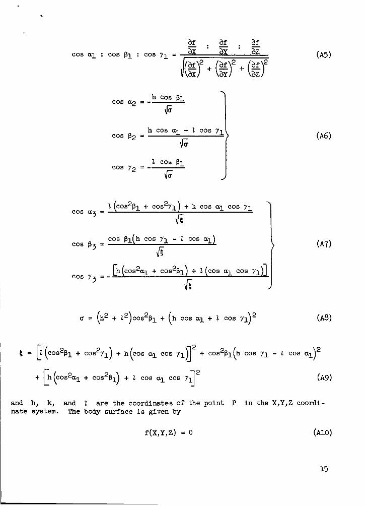
c
h COS f.31 cos a2 = - fi
h COS ul + 2 COS 71 cos $2 =
6 2 cos p 1
6 COS 72 = -
2 (cos2pl + C0S271) + h COS COS 71 cos a3 = G
COS $l(h COS 7'1 - 2 cos ul) cos f33 =
fi [h (cos2al + cos2$1) t 2 (cos a1 cos yl)]
cos 73 = -
JI
and h, k, and 2 are the coordinates of the point P i n the X,Y,Z coordi- nate system. The body surface i s given by
f ( X , Y , Z ) = 0 (A101
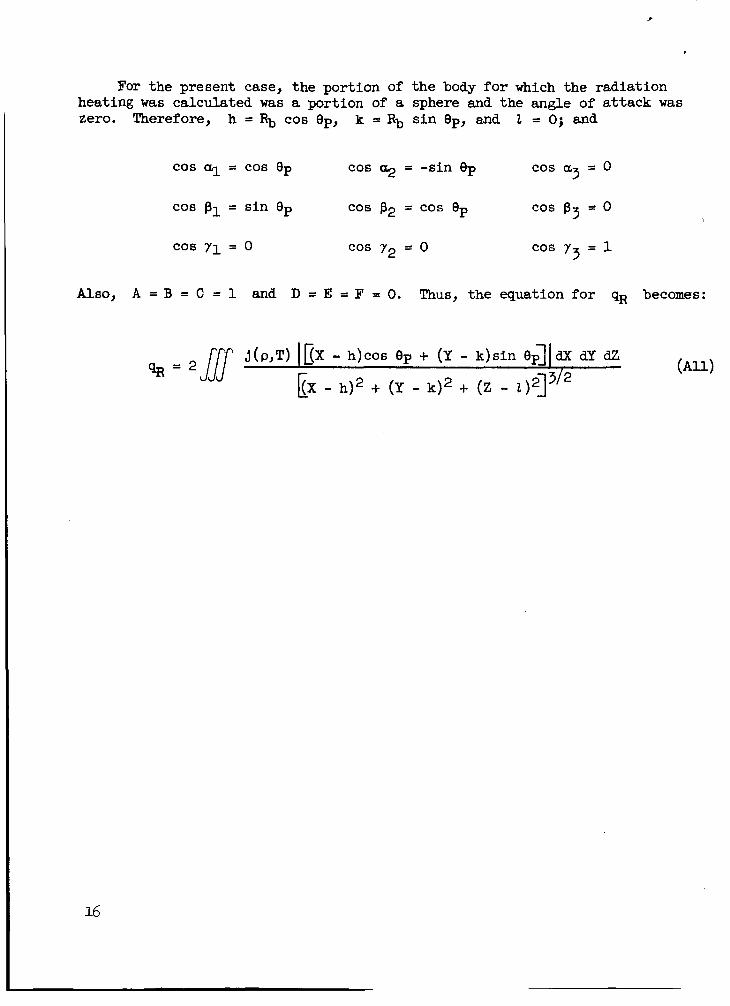
.
For the present case, the portion of the body for which the radiation heating was calculated was a portion of a sphere and the angle of attack was zero. Therefore, h = Rb cos ep, k = Rb sin ep, and 2 = Oj and
cos a = 0 3 cos a1 = cos ep cos 9 = -sin Bp
cos p1 = sin eP cos 82 = cos ep cos p 3 = 0
cos 7 1 = 0 cos r2 = 0 cos r3 = 1
AJ-so, A = B = C = 1 and D = E = F = 0. Thus, the equation for qR becomes:
16
REFERENCES
1. Boison, J. Christopher; and Curtiss, Howard A . : An Experimental Investiga- t i on of B l u n t Body Stagnation Point Velocity Gradient. ARS J., vol. 29, no. 2, Feb. 1959, pp. 130-135.
2. Hayes, Wallace D.; and Probstein, Ronald F.: Hypersonic Flow Theory. Academic Press, Inc. (New York), 1959.
3. Korobkin, I.; and Hastings, S. M.: Mollier Chart f o r A i r i n Dissociated NAVORD Rep. 4446, Equilibrium at Temperatures of 2000' K t o 15000° K.
U.S. Naval Ord. Lab. (White Oak, Ma.), May 23, 1957.
4. Riethof, T.; and Nardone, M.: Radiation Theory. AF 04-(647)-617), Missile and Space Vehicle Dept., Gen. Elec. Co., Aug. 31,
Doc. No. 6 2 ~ ~ 6 8 0 (Contract
1962.
5. Kivel, B.; and Bailey, K. : Tables of Radiation From High Temperature A i r . Res. Rept. 21 (Contracts AF 04(645)-18 and AF 49(69)-61), AVCO Res . Lab., Dec. 1957.
6. Bobbitt, Percy J.: Effects of Shape on Total Radiative and Convective Heat Inputs at Hyperbolic Entry Speeds. Advances i n Astronautical Sci., vol. 13, Eric Burgess, ed., Western Periodicals Co. (N. Hollywood, C a l i f . ), C.1963, PP- 290-3190
1 7. Nardone, M. C.; Breene, R. G.; Zeldin, S. S.; and Riethof, T. R. :
I
Radiance I of Species i n High Temperature A i r .
AF 04(694)-222), Missile and Space Div., Gen. Elec. Co., June 1963. (Available from DDC as AD No. 408564.)
Tech. Inform. Ser. R63SD3 (Contract
8. Beckwith, Ivan E.; and Cohen, Nathaniel B. : t ions t o Calculation of Laminar Heat Transfer on Bodies With Yaw and Large Pressure Gradient i n High-speed Flow.
Application of Similar Solu-
NASA TN D-625, 1961.
9. Cohen, Nathaniel B.: Boundary-Layer Similar Solutions and Correlation Equa- t ions fo r Laminar Heat-Transfer Distribution i n Equilibrium-Air a t Veloc- i t i es up t o 41,100 Feet Per Second. NASA TR R-118, 1961.
h
V P
14
If
10
8
6
4
2
- Total heating measurement
Radiative heating measurements
2 K 10 t = 25 sec; radiation
t = 20 see; calorim- eter experiment - no. 1 data period ends
t = 24 see; f i r s t ablative layer is jettisoned
experiment - no. 2 data period ends
t = 31 see; second \ ablative layer
t = 32 see; radiation experiment - no. 3 data period ends
t = 40 see; calorimeter experiment - no. 3 data period ends
0 io 3'0 5b
Reentry t ime, sec
Figure 2.- Primary data periods showing t o t a l and rad ia t ive stagnation-point heating measurements. ( A t start of reentry, t = 0; a l l times are estimated.)
20
1 .o
.%
.6
P - pi
.4
.2
0 0 .1 .2 .3 .4 .5 .6 .7
S/Rn
Figure 3.- Pressure dist r ibut ions for the various forebcdy configmations.
21
Corner
Figure 4.- Flow-field division f o r reentry vehicle.
22
t
1
.1 .2 .3
S/Rn
Figure 5.- Comparison of l o c a l body radius with e f fec t ive radius. Configuration 2. \
23
10
106
96
94 4 8 12 16 20
0, deg
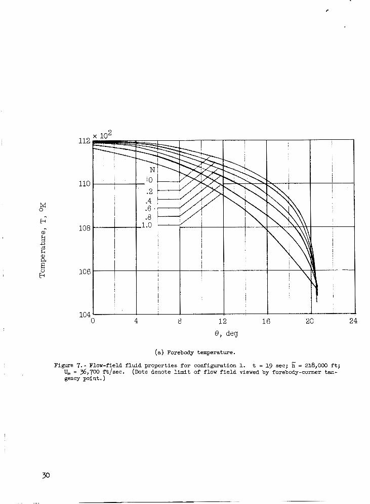
(a) Forebody temperature.
Figure 6.- Flow-field fluid properties for confiwation 1. t = 15 sec; T i = 260,460 ft; U, = 37,058 ft/sec. gency point. )
(Dots denote limit of flow field viewed by forebody-corner tan-
24

I P 8 -
I ps1
36 x lo-+ I !
32
28
24
20
16
i !
I i s
4 a 12 16 20 24 6 , deg
(b) Forebody density.
Figure 6.- Continued.
25
J
.10
.08
I 0)
E 0; \ .04 3
.02
+ I
I
!
I 4 12 16 20 C
L
8 , deg
(c) Forebody specific radiation intensity.
Figure 6.- Continued.
26
20 40 60 80 100 0
e,, deg
(a) Corner temperature.
Figure 6.- Continued.
27
P - Psi
' I !
I ' I 0 I I
0 20 40 60 eC, deg
(e) Corner density.
Figure 6.- Continued.
80 100
28
c
112 I O 2
110
108
106
104 0 4 8 12 16 20 24
( a ) Forebody temperature.
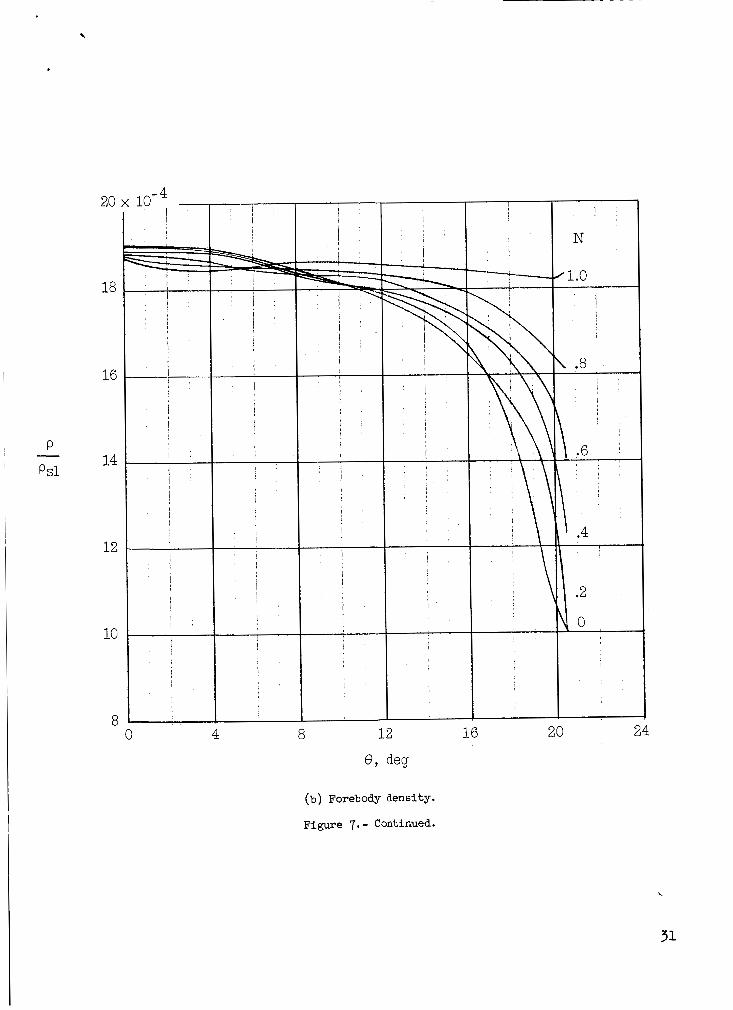
Figure 7.- Flow-field f l u i d propert ies f o r configuration 1. t = 19 sec; - h = 218,000 f t ; U, = 36,700 f t /sec. gency point. )
(Dots denote l i m i t of flow f i e l d viewed by forebody-corner tan-
20 I
18
16
P 14 -
~ P s l
I
N
11.0
12
10
a
, \ I
j I s , I j i
.2
0
0 4 8 12 16 20 24
8 , deg
(b) Forebody density.
Figure 7.- Continued.
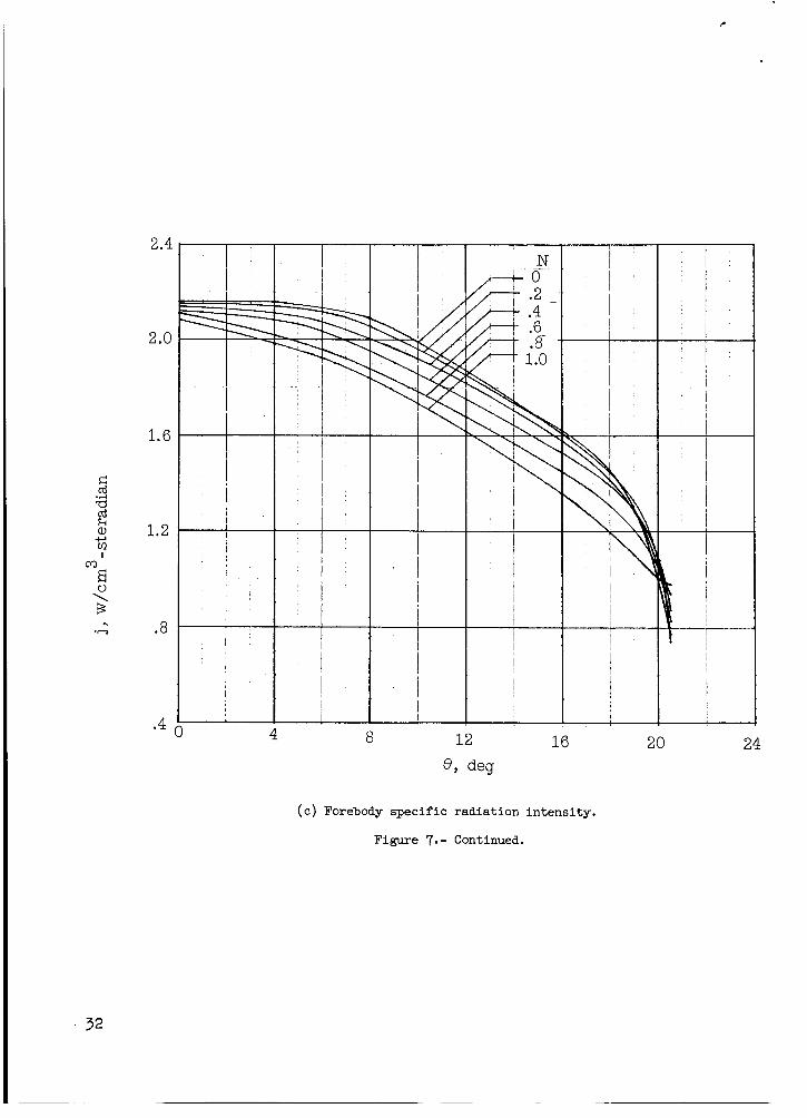
2.4
2.0
1.6
.4
32
I
I I N I +
4
I 1
I
8 12
0, deg 16
I
-j-
!
--- I
(c) Forebody specific radiation intensity.
Figure 7.- Continued.
20 24
k4 0
11
10
9
8
7
6
3 12 x 10- I I
, I
I I
I ,
i j
I
0 20
I
i N j j 0.E
I ’
I
1 I I
. I
\ I I ‘ i
I I
!
I
.
I
80 100
(d) Corner temperature.
Figure 7.- Continued.
33
28
24
20
16
12
8
4
0
-
i I
+- L
I
-7- I I
-I-
20 40 60 g,, deg
80 100
(e) Corner density.
Figure 7.- Continued.
34
2 .o
1.6
1.2
.8
.4
0 20 40 60 80 100 e,, deg
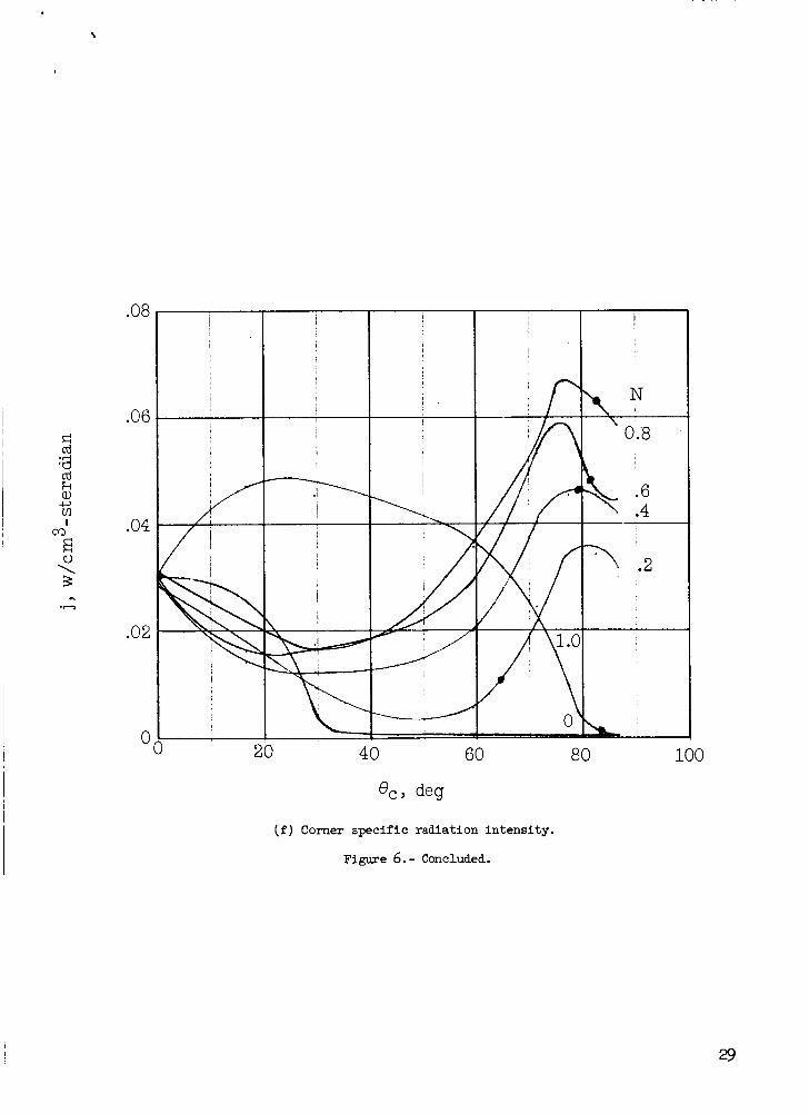
(f) Corner specific radiation intensity.
Figure 7.- Concluded.
35
h
J u 0 4 8 16 20 24
(a) Forebody temperature.
Figure 8.- Flow-field f l u i d propert ies f o r configuration 2. t = 25 sec; E = 166,000 ft; U, = 34,800 f t / sec . gency point. )
(Dots denote l i m i t of flow f i e l d viewed by forebody-corner tan-
0 4 8 16
N
1.0
\
.8
.2
0
20 24
(b) Forebody density.
Figure 8.- Continued. I
37
2E
24
20
I I
I
i I
8
I I
, !
I
4
I 1 j
4
I
!
I I I i !
I
\ I
i j
8 16
I
20 24
(c) Forebody specific radiation intensity.
Figure 8.- Continued.
38
12 x
10
8
6
4
2 0 20 40 60 80 100
e,, deg
(a) Corner temperature.
Figure 8.- Continued.
39
P
Psi
14 x
1:
1(
f
4
2
0 0 20
t 40 60
8c, deg
\ L O !
I
.8
'\, .6 .4 \
.2
- 0
80 100
(e) Corner density.
Figure 8.- Continued.
12
10
8
3 cd k a, m 6 4
I m
E
3 0 \
- 4 e n
2
0
i I i i I '
I __t__
I
I
c i
. .
I I
1
- N -
0 20 40 60 80 100 e,, deg
(f) Corner specific radiation intensity.
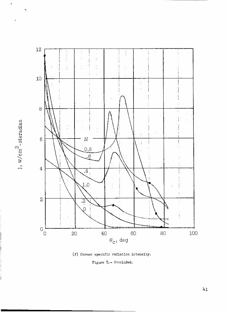
Figure 8.- Concluded.
41
a E 8
76
72 0 4 a 12
9, deg 16 20
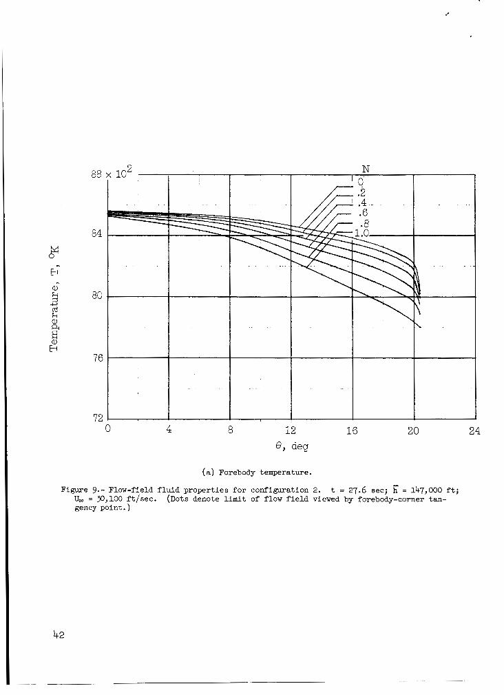
(a) Forebody temperature.
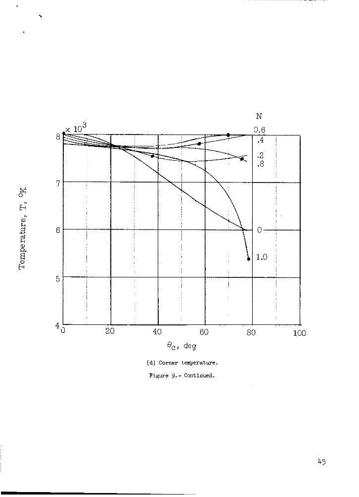
Figure 9.- Flow-field f l u i d propert ies f o r configuration 2. t = 27.6 sec; = 147,000 f t ; U, = 30,100 f t / s ec . gency point. )
(Dots denote l i m i t of flow f i e l d viewed by forebody-corner tan-
24
42
3 32 x lo ' , -
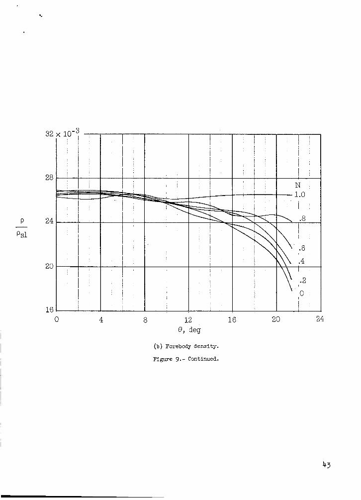
28
P 24 - p sl
20
16
I I I
I I I
0 4 8 12 16 20 24 e , deg
(b) Forebody density.
Figure 9.- Continued.
43
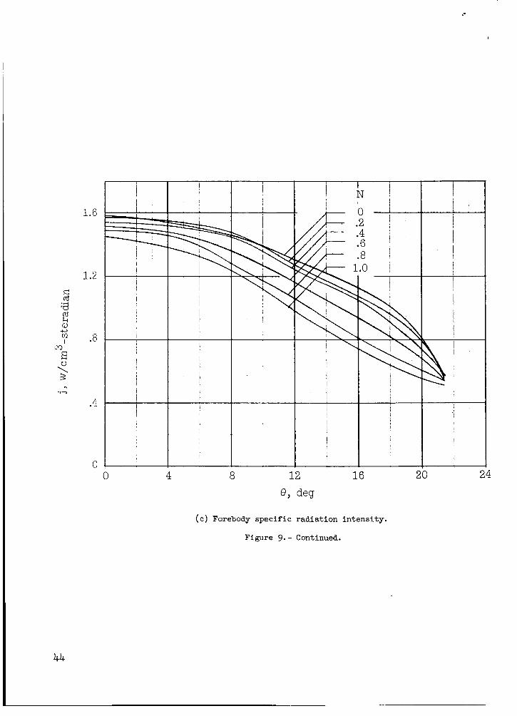
1.6
1.2
0 0 4 8 12
9, deg
16 20 24
(c) Forebody specific radiation intensity.
Figure 9.- Continued.
44
20 40 60
e,, deg
(d) Corner temperature.
Figure 9.- Continued.
N 0.6 .4 i
.2
.8
1.0 I
80 100
45

46
P
Psi -
28 x
24
20
16
12
8
4
- I I
i -I- \ '.\\\ \ !
20
I
i 1 i 1 i 8
I I
I
1 .o
!
I
.6 ~
i .4 I
.2 1 +-- o j
a0 100
(e) Corner density.
Figure 9.- Continued.
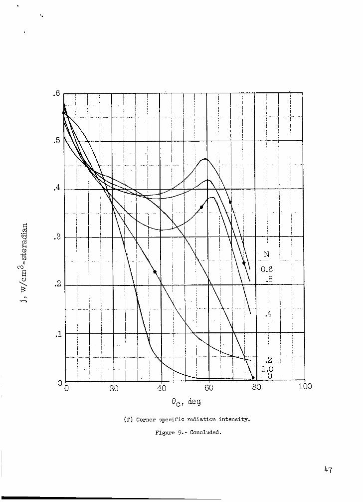
.6
.5
.4
LT: cd
cd k a, 4 m
I m
3 .3
E
3 < .2 - e n
.1
O O 20 40 60 80 l
e,, deg
( f ) Corner specif ic radiation intensi ty .
Figure 9.- Concluded.
47
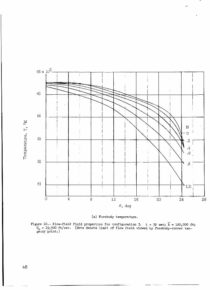
66 x
65
64
63
62
61
8 12 16 20 24 28 6 , decJ
(a) Forebody temperature.
Figure 10.- Flow-field fluid properties for configuration 3. t = 32 sec; I; = 120,000 ft; U, = 19,500 ft/sec. gency point. )
(Dots denote limit of flow field viewed by forebody-corner tan-
48
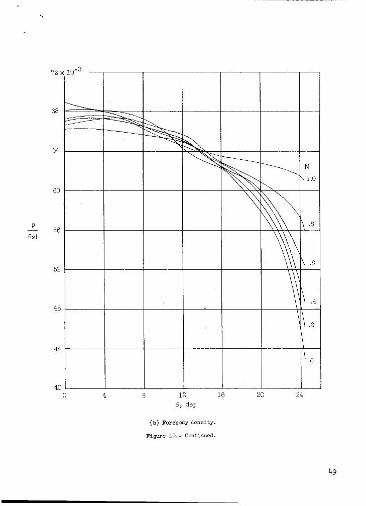
n
72
sa
64
6C
5f P
Psi -
5:
4(
4z
4( 0 4 a 12 16 20 24
8, deg
(b) Forebody density.
Figme 10. - Continued.
49
.32
.28
.24
.20
.16
.12
.08 0 4 8 16 20
I
c L
(c) Forebody specific radiation intensity.
Figure 10. - Continued.
w 0
68
64
60
56
52
48
44
lo2 -
I !
I
I
0 20
,
I
I
I
I
! , i
40 60 e,, deg
N
3.6
1 .o \
80 1 3
(a) Corner temperature.
Figure 10. - Continued.
20 40 60 80 100 e,, deg
(e) Corner density.
Figure 10. - Continued.

.12
.1c
.OE
d cd
cd k a, u1
3
.OE 4
I rn E
3 < -
.04 *m
.02
0
I
1 I
' I ' I
I 1
N
I ' I I
o i - 80 1
(f) Corner specif ic radiation intensi ty .
Figure 10. - Concluded.
53
*
I d
54
qR’ Btu
sec-ft 2
.o
- Figure 12.- Convergence of radiat ion heating equation. t = 25 sec; h = 166,000 ft;
U, = 9,800 f t /sec; ep = 0 .
55
qR, t
1.2
1.01
.8
.6
.4
.2
0
I
l--
' ! i
---4---
!
I i
, , 8 1
0 0 .
0 4 8 12 16 20 c 1
Q, deg
56
- (a) t = 15 sec; h = 260,460 ft; LJ, = 37,058 ft/sec.
Figure 13.- Radiation heat-transfer distribution.
- ‘R ‘R, t
I
0 Present method Slab approximation
4
(b) t = 19
8 12 0, deg
- see; h = 218,000 ft; U, =
Figure 13. - Continued.
20
ftlsec.
24
37
1.2
1.0
.8
__ gR .6
qR, t
.4
.2
0 0
\
* Present method 0 Slab approximation
4 8 12 16 8 , deg
- (c) t = 25 sec; h = 166,000 ft; U, = 9,800 ft/sec.
Figure 13. - Continued.
20 24
58
.2
0 0 4 8 1 2 1
8 , deg
0 Present method 0 Slab approximation
-
~
2
t--
2
(a) t = 27.6 sec; = 147,000 ft; U, = 31,100 ft/sec.
Figure 13. - Continued.
59
1.2
1.0
.a
- qR .6 ‘R, t
.4
.2
8 12 16 20 24 28 0, deg
Figure 13. - Concluded.
60
I 0 0 8 5:
- _ - -
. . . -
_ - - -
G- O
00
I I
_ - -
\
bD \ \ \ \
* d d 0 Pi
0 *
I
61
1000
800
600
qR, t’ B tu
2 see-ft 400
200
0 Reference 4 Reference 5 Reference 7
(a) Stagnation-point vdue.
Figure 15.- Comparison of radiatis heating using various values for specific intensity. t = 25 sec; h = 166,000 ft; U, = 34,800 ft/sec.
62
1.0(
.8
.6
- qR
qR, t .4
.2
0
0 Reference 4 0 Reference 5
8 12 e , deg
16
(b) Heat-transfer distribution.
Figure 15.- Concluded.
20 24
0 .2 .4 .6 .8 1 .o 1.2
(a) t = 15 sec; E = 260,460 ft; U, = 37,058 ft/sec.
Figure 16.- Convective heat-transfer distribution.
64
1.2
1.0
.8
- qC .6 qc, t
.4
.2
0
-1/ I
I
0 .2 ,4 .6 .8 1 .o n s/R
- (b) t = 19 sec; h = 218,000 ft; U, = 36,700 f t /sec.
Figure 16. - Continued.
2
.'
1.2
1 .o
.a
.4
.2
0 0
I
!
1
.2
2orner -j 1.2 .4 .6
S/Rn .8 1 .o
( c ) t = 25 sec; = 166,000 f t ; U, = 9,- ft /sec.
Figure 16. - Continued.
66
1.2
1 .o
.8
.4
.2
2 Zomer
.4 .6 s/Rn
.8 1 .o
(d) t = 27.6 sec; = 147,000 f t ; U, = 31,100 f t / sec .
Figure 16. - Continued.
1.2
67
1.2
1 .o
.8
- qC .6
qc, t
.4
.2
0 ( .4 .6 .8 1 .o 1.2
n S/R
- ( e ) t = 32 sec; h = 120,000 ft; U, = 19,500 ft/sec.
Figure 16. - Concluded.
68
0 0 0 0 (SI a3
0 0 0 dl
1000
800
u
200
0
t = 25 sec - m U = 34,800 ft/sec h = 166,000 f t 7
U, = 34,582 ft/sec \ E = 171,111 f t
= o = 2800 OR
t = 15 sec - urn= 37,058 ft/sec h = 260,460 f t
(a) Stagnation-point convective heating rate.
Figure 18. - Comparison between heating rates and heating distributions.
L '3aH
0 0 0 2 23
4
L .- . .
0 52
0 a,
+ w
.- 0 a, I s
I I 0 4 0 8 8 9
h
v P
1.2
1.0
. 8
I_ qC . 6 qc, t
. 4
. 2
0 0
Philco -
.1 . 2 S
.3
Corner
(c) Convective heat-transfer distribution.
Figure 18.- Continued.
. 4 . 5
72
1 . 2
1.0
. 8
-- qR .6 qR, t
. 4
.2
0 0
. - .. - --_ . ..
__..I_-
\- - -
,G . E.
Present report
4 8 12 16 20 4
0, deg
(d) Radiative heat-transfer d i s t r ibu t ion .
Figure 18. - Concluded.
73
x
74
\ \
a \
/ '
' I /
/ I /
/ I I
/ I
N
NASA-Langley, 1965 L-4091