measurements and predictions of the heat transfer at the ... · measurements and predictions of the...
TRANSCRIPT

Measurements and Predictions of the Heat Transfer at the Tube-Fin
Junction for Louvered Fin Heat Exchangers
Christopher P. Ebeling, Graduate Research Assistant Virginia Tech, Mechanical Engineering Department
Blacksburg, VA 24061 (540)231-4775
K.A. Thole, Professor* Virginia Tech, Mechanical Engineering Department
Blacksburg, VA 24061 (540)231-7192 [email protected]
Submitted for review to the International Journal of Compact Heat Exchangers, May 2003

2
Measurements and Predictions of the Heat Transfer at the Tube-Fin
Junction for Louvered Fin Heat Exchangers
Abstract
The dominant thermal resistance for most compact heat exchangers occurs on the air side
and thus a detailed understanding of air side heat transfer is needed to improve current designs.
Louvered fins, rather than continuous fins, are commonly used to increase heat transfer by
initiating new boundary layer growth and increasing surface area. The tube wall from which the
fins protrude has an impact on the overall heat exchanger performance. The boundary layer on
the external (typically, air) side of the tube is subjected to repeated interruptions at the louver-
tube junction. This paper discusses baseline results of a combined experimental and
computational study of heat transfer along the tube wall of a typical compact heat exchanger
design. A scaled-up model of a multi-louver array protruding from a heated flat surface was
used for the experiments. The results of this study indicate reasonable agreement with steady,
three-dimensional computational predictions.

3
1. INTRODUCTION
Understanding the mechanisms that dominate heat transfer in a louvered fin heat
exchanger provides the potential for reducing the heat exchanger’s size and weight. This
reduction in size can clearly benefit many industries, including transportation, heating, and air
conditioning. Because more than 85% of the total thermal resistance in a typical air-cooled heat
exchanger occurs on the air side, the performance of compact heat exchangers depends highly on
the heat transfer occurring on the air side.
Louvered fins, rather than continuous fins, are commonly used in compact heat
exchangers to break up boundary growth along the fins and increase the air side heat transfer
surface area. The increase in surface area results because of the fin thickness that is exposed as a
result of the louvers being stamped out of the fins. Figure 1 illustrates a typical compact heat
exchanger geometry comprised of louvered fins, where air passes along, and tubes, where water
passes through. Unlike most studies concerning louvered fin heat exchangers, this study focuses
on the spatial details of the flow and local heat transfer of these louvers at the louver-tube
junction. The louver-tube junction influences compact heat exchanger performance in two ways:
first the tube wall provides approximately 10% of the total heat transfer surface area, and second,
the tube wall boundary layer governs a portion of the fin heat transfer near the junction. Even
though the tube wall consists of only 10% of the total heat transfer surface area, several
geometric aspects of the tube-fin junction serve to reduce resistance on the air side. Unlike
continuous fins, louvered fins interrupt the boundary layer growth along the tube wall, which
could be thought of as a flat plate. Generally, the aspect ratio of the tubes is such that the tube
wall boundary layers do not intersect and the flow can be thought of as an external flow. The
interruption of the louvers governs the thickness of the tube wall boundary layer and affects the
tube wall heat transfer as well as fin performance near the junction.
This paper presents results of a combined experimental and computational study of tube
wall heat transfer with the wall being subjected to boundary layer interruptions from the louvered
fins. The experiments were performed in a test rig with a scaled-up model of the louver-tube
junction, which was simulated as a heated flat plate with nearly adiabatic louvers protruding
from the plate. Studies were performed for one louver fin geometry, specifically for a ratio of fin

4
pitch to louver pitch of Fp/Lp = 0.76 at a louver angle of θ = 27o and Reynolds number range of
230 < Re < 1016 where Re is based on the inlet velocity and the louver pitch.
1.1 Literature Review
The overall performance of various compact heat exchanger geometries are found in a
large number of publications. Since the majority of this data focuses on heat exchangers as an
entire system, ε-NTU and LMTD methods are often applied. Kays and London (1984) compiled
overall performance data, including heat transfer and pressure drop, for a large number of
commercial heat exchangers. While this compilation is extremely useful to heat exchanger
companies, the data does not present details on the individual flow field and heat transfer
mechanisms that occur within each heat exchanger design. A few studies will be highlighted in
this section, which provide insights as to the important mechanisms affecting the louver heat
transfer.
Most studies that have evaluated the details of heat transfer for a louvered surface have
been completed in two-dimensional test rigs whereby the area of interest has been along the
louver surface itself. Beauvais (1965) performed detailed experiments with the use of smoke
visualization and showed how the louvers direct the air flow under certain conditions and
geometries (louver directed) as opposed to the flow being axially directed. The experiments of
Beauvais disposed of the idea that the main flow direction was axial and that the louvers only
acted as rough surfaces within the main flow. By repeating Beauvais’ experiments, Davenport
(1983) was able to show the degree to which the flow is louver directed. Davenport noticed that
louver directed flow is a function of Reynolds number. At low Reynolds numbers, the flow
tended to remain axially directed, whereas at higher Reynolds numbers the flow tended to
become louvered directed.
In general, later studies of Webb and Trauger (1991) identified that the flow tends to be
louver directed at high Reynolds numbers, low louver angles, and large fin pitches. Achachia and
Cowell (1988) investigated overall heat transfer and friction factors for a large range of louvered
fin geometries. They found that at Reynolds numbers below 200, heat transfer performance
flattened off considerably. This tendency was attributed to the flow remaining axially directed. In
contrast, as the flow becomes louver directed at high Reynolds numbers, the overall average heat
transfer coefficients increase above that of the axially directed flow.

5
Fewer studies have addressed three-dimensional effects in louvered fins relevant to
compact heat exchangers. Flow visualization studies by Namai, et al. (1998) were completed in
which three-dimensional fin models were used. These three-dimensional models included
several different geometries at the tube-wall junction. Their overall conclusions were that there
are strong three dimensional characteristics in louvered fin flows. Atkinson, et al. (1998)
performed computational simulations of both two and three-dimensional models whereby the
three-dimensional model included the effects of the tube. Their results indicated that the three-
dimensional models gave predictions that were in better agreement with experimental
observations of both pressure losses and heat transfer reported by Achachia and Cowell as
compared with their two-dimensional predictions. Tafti, et al. (2000) solved three-dimensional
computational models of multilouvered fins for a fully-developed flow and predicted a number
of interesting flow features at the tube-wall junction. Their study incorporated a geometric
transition zone between the louver and the tube wall that served to produce vortices such that the
heat transfer was increased along the louver. In later studies, Taft and Cui (2002) investigated the
effects the transition zone had on tube wall heat transfer. It was found that by creating a high
energy vortex jet, the transition zone significantly increases tube wall heat transfer. As an
extended study, Taft and Cui (2003) repeated their previous investigation into the transition
zone’s impact on the heat transfer at the tube wall for four different geometries. Their baseline
geometry was composed of a straight louver-tube junction with no transition zone, similar to the
geometry studied in this investigation. However, the studies of Taft and Cui (2002 and 2003)
consider only fully-developed flow conditions and ignore the effects at the entrance, reversal,
and exit louvers.
Since the performance of compact heat exchangers is directly governed by the air side
flowfield, it is important to understand the fluid structures that exist. Because publications of the
heat transfer in the developing regions along the tube wall with protruding fins are non-existent,
the work presented in this paper was warranted.

6
2. EXPERIMENTAL METHODOLGY
The studies discussed in this paper were performed on a louvered fin and tube design as
was illustrated in figure 1 and summarized in table 1. Louvered fins are typically stamped and
bent to meet the design louver angle (θ), louver pitch (Lp), and fin pitch (Fp) before being
attached to the tube. Once attached to the tubes, the ends of the louvers create the tube-fin
junction. Our model does not include any type of transition from the louver to the tube wall, but
rather a direct contact between the louver and tube wall.
The flow facility used for the study, except for the test section, was identical to the set-up
reported by Lyman et al. (2002). As shown in figure 2, the flow facility primarily consisted of an
inlet contraction, a louvered fin test section, a laminar flow element, and a centrifugal blower.
The inlet contraction, which had a 16:1 area reduction, was designed through the use of
computational fluid dynamics (CFD) simulations in which the goal was to provide a uniform
velocity profile at the inlet to the test section. This uniformity was verified through laser
Doppler velocimeter measurements by Lyman (2000). A variable speed centrifugal blower
located at the exit of the test rig provided the flow through the test rig with the speed of the
blower being controlled using an AC inverter. The flow rate was measured using a laminar flow
element (LFE) located just downstream of the test section.
The louvered fin test section, which was designed to measure the heat transfer along a
wall with protruding louvers, was constructed as shown in figure 3. Note that this test section is
designed to follow the flow path, which was shown to be primarily louver directed, such that an
infinite stack of louvers are simulated (Springer and Thole, 1998). Balsa wood louvers, painted
silver, were used to reduce any conduction and radiation losses from the wall heat transfer
surface. The silver paint used to coat the balsa wood louvers and the black paint used to coat the
tube wall had emissivities of 0.3 and 0.98, respectively (Siegel and Howell, 1981). The louvers
were held in position by inserting them into milled slots in a lexan wall on one side of the test
section and inserting them into specially designed, low thermal conductivity lexan plugs glued
onto the heat transfer surface on the other side of the test section. Glued plugs, rather than slots,
were needed on the side having the heat flux surface because the foils on that surface could not
be slotted. The louvered fin plugs were made of lexan and held balsa wood louvers at the tube
wall. The combination of lexan plugs and balsa wood louvers provided reduced heat loss through

7
the louvers at the louver-wall junction. Defined as ( ) 21
f,cffff Ah / Pkη = , the fin effectiveness for
an infinitely long fin was calculated to ensure losses through the fin were negligible. The
infinitely long fin assumption was valid since CFD studies predicted that 85% of the louver’s
width was outside the tube wall’s thermal boundary layer. For the smallest averaged heat transfer
coefficients along the louver, fh (Lyman et al. 2002), the fin effectiveness for Re = 230 and 1016
were fη = 2 and 1.8, respectively. These values represent the largest fin efficiencies expected
within the test section. Since the use of fins are rarely justified unless fη > 2, it was assumed that
balsa wood fins were ineffective in conducting heat from the tube wall.
A constant heat flux boundary condition was placed on the experimental tube-wall by
using heating foils, as was indicated in figure 3. This heated surface started at the leading edge
of the entrance louver, where X = 0. To create the heat transfer surface, we attached stainless
steel foil heaters to a lexan sheet with double-sided tape. Each strip heater was cut from 0.0508
mm thick grade 316 stainless steel foil with nominal electrical resistance of 74 µΩ-cm. To
ensure uniform current distribution through the foils and provide a terminal for lead wires
soldered copper bus bars 1.58 mm thick were soldered to the foil. The tube wall required twenty
foil heaters having a width of 28 mm and height of 295 mm to completely cover the flat wall
from entrance to exit louver. All strip heaters were connected in series to provide a constant
current through the heater circuit. The resistances of the strip heaters were calculated by
applying a current to the foils and measuring the resulting voltage drop. 20 different foils were
sampled showing that each had a nominal resistance of R = 0.14 Ω ± 1%. We considered the
power output to be equal as a result of this resistance uniformity. Current through the heater
circuit was determined by measuring the voltage drop across a precision resistor, Rp =1Ω ± 1%,
connected in series with the heater circuits. Knowing the voltage drop and resistance, the total
power dissipated was calculated. The surface area of the strips was also known thereby
providing the known total heat flux from the strips.
To minimize the effects of heat losses due to conduction and radiation, two guard heaters
were included in the test section design. Both guard heaters consisted of two patch heaters taped
to an aluminum plate that was encased in an insulating wooden box. The aluminum plate served
to spread out any temperature gradients that might have existed between the patch heaters. Each
guard heater was instrumented with thermocouples located at the same wall location as the center
8
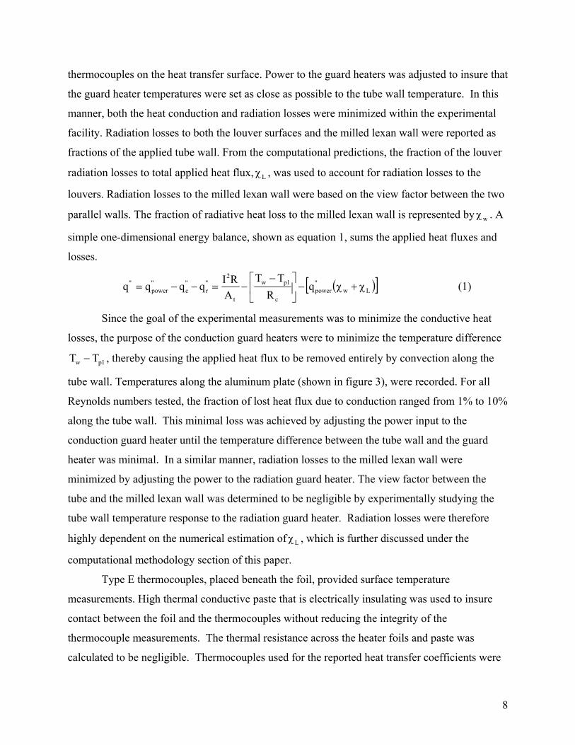
thermocouples on the heat transfer surface. Power to the guard heaters was adjusted to insure that
the guard heater temperatures were set as close as possible to the tube wall temperature. In this
manner, both the heat conduction and radiation losses were minimized within the experimental
facility. Radiation losses to both the louver surfaces and the milled lexan wall were reported as
fractions of the applied tube wall. From the computational predictions, the fraction of the louver
radiation losses to total applied heat flux, Lχ , was used to account for radiation losses to the
louvers. Radiation losses to the milled lexan wall were based on the view factor between the two
parallel walls. The fraction of radiative heat loss to the milled lexan wall is represented by wχ . A
simple one-dimensional energy balance, shown as equation 1, sums the applied heat fluxes and
losses.
( )[ ]Lw"power
c
1pw
t
2"r
"c
"power
" qR
TTA
RIqqqq χ+χ−
−−=−−= (1)
Since the goal of the experimental measurements was to minimize the conductive heat
losses, the purpose of the conduction guard heaters were to minimize the temperature difference
1pw TT − , thereby causing the applied heat flux to be removed entirely by convection along the
tube wall. Temperatures along the aluminum plate (shown in figure 3), were recorded. For all
Reynolds numbers tested, the fraction of lost heat flux due to conduction ranged from 1% to 10%
along the tube wall. This minimal loss was achieved by adjusting the power input to the
conduction guard heater until the temperature difference between the tube wall and the guard
heater was minimal. In a similar manner, radiation losses to the milled lexan wall were
minimized by adjusting the power to the radiation guard heater. The view factor between the
tube and the milled lexan wall was determined to be negligible by experimentally studying the
tube wall temperature response to the radiation guard heater. Radiation losses were therefore
highly dependent on the numerical estimation of Lχ , which is further discussed under the
computational methodology section of this paper.
Type E thermocouples, placed beneath the foil, provided surface temperature
measurements. High thermal conductive paste that is electrically insulating was used to insure
contact between the foil and the thermocouples without reducing the integrity of the
thermocouple measurements. The thermal resistance across the heater foils and paste was
calculated to be negligible. Thermocouples used for the reported heat transfer coefficients were

9
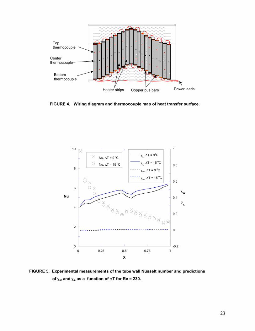
positioned in the center of the channel, shown as black dots in figure 4, while periodicity was
checked by recording the temperatures above and below the center thermocouples, shown as red
dots in figure 4.
The thermocouples were accurately calibrated relative to one another in an ice bath and at
room temperature. Thermocouple biases remained constant to within 0.19 oC over a temperature
range of 25 oC. Data acquisition hardware used to acquire the thermocouple voltages consisted of
a National Instruments SCXI-1000 chassis into which three SXCI-1102 modules were inserted.
An SXCI-330 terminal block was inserted into each of the modules. The data sample size to
compute the mean temperatures consisted of 100 data points, which were acquired after the test
surface came to steady state. It typically took 3 hours for the test section to reach steady state.
The uncertainties of experimental quantities were estimated by using the method
presented by Moffat (1988). The uncertainty was calculated by acquiring the derivatives of the
desired variable with respect to individual experimental quantities and applying known
uncertainties. The combined precision and bias uncertainty of the individual temperature
measurements was ± 0.19 ºC, which dominated the other uncertainties. The uncertainties in the
Nusselt numbers for the Re = 230 was 8% at strip 1, which fell to 4.8% at strip 20. The reduction
in uncertainty is contributed to a larger temperature difference between the tube wall and free
stream as the tube wall boundary layer develops along the X-direction. Similarly, for the Re =
1016 flow condition, the uncertainties in the Nusselt numbers ranged from 8% at strip 1 to 5.9%
at strip 20. Uncertainty of the Reynolds numbers ranged from 3.3% at Re = 230 to 1.9% at Re =
1016. Reynolds number uncertainties were primarily due to acquiring an accurate volumetric
flow rate from pressure drop measurements across the LFE.
3. COMPUTATIONAL METHODOLOGY
Three-dimensional computational simulations were completed using the commercial
package (Fluent 6.1, 2002). Fluent is a pressure-based, incompressible flow solver that can be
used with structured or unstructured grids. CFD predictions were obtained by solving the
momentum equations, energy equation, and the radiation transport equation (RTE), using second
order discretization. The flow was simulated as three-dimensional, laminar, and steady. To
10
replicate the experiments, a single row of 17 streamwise louvers, including one entrance louver,
one reversal louver, and one exit louver, made up the computational domain. Periodic boundary
conditions were used to computationally simulate the infinite stack of louvers. The inlet to the
computational domain was located 3 louver pitches upstream of the entrance louver while the
exit was located 6.5 louver pitches downstream of the exit louver. A constant velocity boundary
condition was applied to the inlet at the matched Reynolds numbers. The exit to the fin channel
was assigned an outflow boundary condition. A constant heat flux was applied to the tube wall
(flat plate) surface and a symmetry boundary condition was applied at the channel’s midspan.
The louver surfaces and the tube wall were assigned emissivity values of 0.3 and 0.98 to
replicate the silver louvers in the experimental test section. Since the effectiveness of the louvers
was calculated to be small, the base of the louvers was considered to be adiabatic.
To ensure a high quality mesh, several steps were taken. First, a quadrilateral grid was
attached along the tube wall surface. This grid allowed for higher resolution along the heat
transfer surface while capturing the tube wall boundary layer. Through previous simulations, the
tube wall boundary layer thickness was computed; thus, the depth of quadrilateral meshing was
known. Second, the volume of the channel was meshed using an unstructured scheme with
constant grid density.
Grid insensitivity was obtained through a number of grid density studies. These studies
included repeatability of the predictions of the heat transfer at the tube wall. Five adaptations on
velocity and temperature gradients rendered a final grid containing approximately 2.2 million
cells. The difference in the average tube wall Nusselt number between the initial mesh
(consisting of 1.1 million cells) and the final mesh was 7%. Further grid independency studies
were limited by computational memory restrictions. The convergence criterion used was that
residuals for u, v, w, and continuity dropped by four orders of magnitude and seven orders of
magnitude for energy and radiation intensity. All computations were performed in parallel and
required approximately 250 iterations to ensure convergence.
3.1 Radiation Modeling
Radiation exchange between the tube wall and the louvers required that additional
radiation modeling needed to be included with the CFD predictions. Fluent’s Discrete Ordinates
(DO) model solves the radiation transfer equation for a discrete number of finite solid angles. By

11
including the DO model, the intensity of radiation at any position along a path through an
absorbing, emitting, and scattering medium is accounted for. Although scattering and absorption
through air was minimal, the emissivity of the louvers posed a potential for radiation absorption.
The discretized version of the RTE in the DO model, directly accounts for directional
dependence of radiation exchange to the louver surfaces, therefore accounting for radiation
absorption within the louver array. Convergence of the DO model required two iterations of the
RTE per flow iteration.
Credibility in the DO model was obtained by experimentally comparing the tube wall
Nusselt numbers for different ∆T conditions. ∆T is the temperature difference between the local
surface temperature of strip heater 1 and the inlet air temperature. By adjusting the surface heat
flux to the tube wall, the desired ∆T condition was obtained. All experiments were conducted at
a ∆T of approximately of 9 oC. For the lowest Reynolds number investigated, Re = 230,
experimental tests were conducted at both ∆T = 9 oC and 15 oC. By conducting the experiment at
Re = 230 and ∆T =15 oC , calculation of the tube wall Nusselt number from equation 1 was
more dependent on predictions of Lχ than in any other case. The ability of the DO model to
accurately predict the radiation losses for different ∆T conditions is well illustrated in figure 5.
As illustrated, the DO model predicts lager values of Lχ for the larger ∆T case. The repeatability
in Nusselt number, as shown in figure 5, verifies that radiation losses to the louvers can be
directly accounted for as expressed in equation 1.
4. EXPERIMENTAL AND COMPUTATIONAL RESULTS
Heat transfer measurements and predictions were made along the tube wall for three
different inlet Reynolds numbers (Re = 230, 625, 1016). Nusselt numbers, based on the louver
pitch, were used to compare the tube wall heat transfer coefficients. Since experimentally the
tube wall consisted of twenty strip heaters, each instrumented with one center thermocouple,
experimental measurements of heat transfer represent the local heat transfer at the center of the
strip. All heat transfer coefficients were based on using the inlet air temperature as the reference
temperature.
12
4.1 Tube Wall Heat Transfer Coefficients
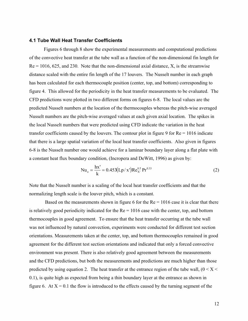
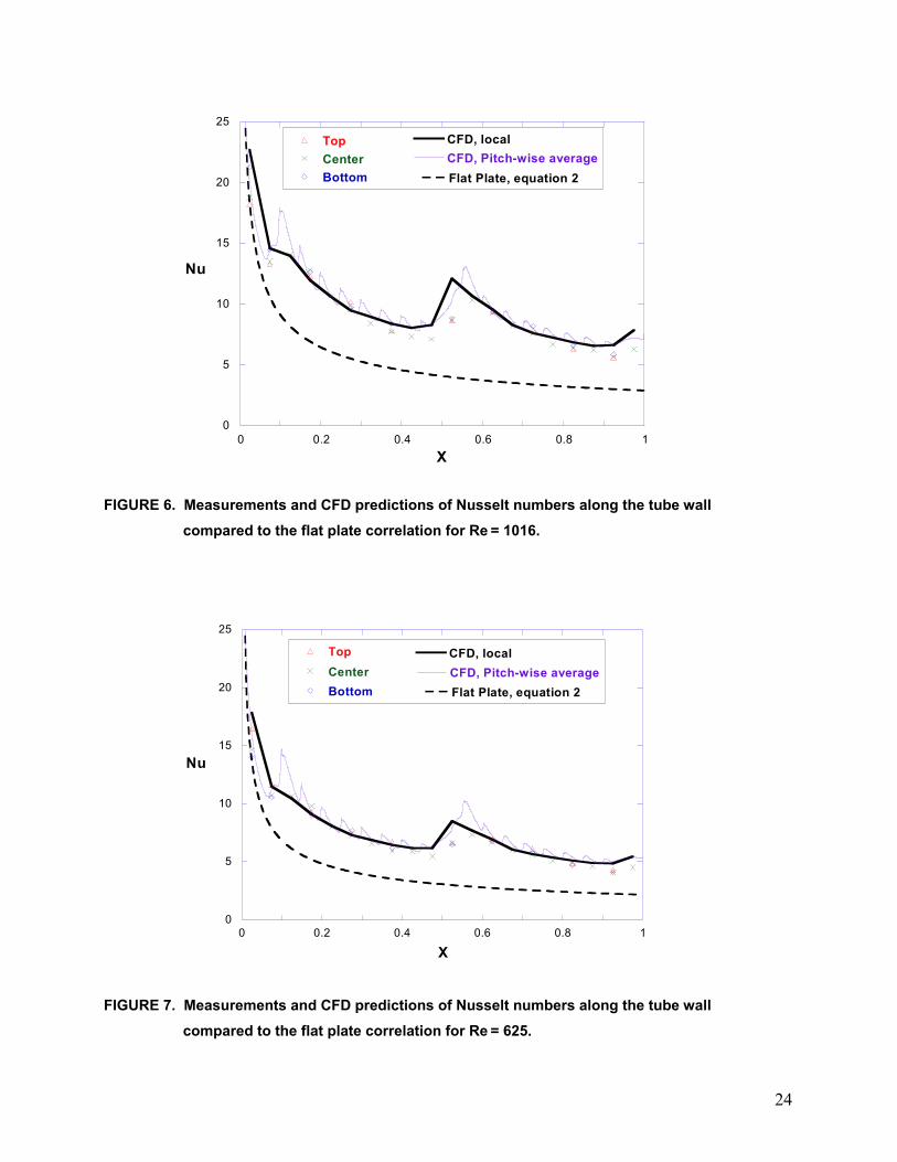
Figures 6 through 8 show the experimental measurements and computational predictions
of the convective heat transfer at the tube wall as a function of the non-dimensional fin length for
Re = 1016, 625, and 230. Note that the non-dimensional axial distance, X, is the streamwise
distance scaled with the entire fin length of the 17 louvers. The Nusselt number in each graph
has been calculated for each thermocouple position (center, top, and bottom) corresponding to
figure 4. This allowed for the periodicity in the heat transfer measurements to be evaluated. The
CFD predictions were plotted in two different forms on figures 6-8. The local values are the
predicted Nusselt numbers at the location of the thermocouples whereas the pitch-wise averaged
Nusselt numbers are the pitch-wise averaged values at each given axial location. The spikes in
the local Nusselt numbers that were predicted using CFD indicate the variation in the heat
transfer coefficients caused by the louvers. The contour plot in figure 9 for Re = 1016 indicate
that there is a large spatial variation of the local heat transfer coefficients. Also given in figures
6-8 is the Nusselt number one would achieve for a laminar boundary layer along a flat plate with
a constant heat flux boundary condition, (Incropera and DeWitt, 1996) as given by:
( ) 33.05.0'Xo PrRe'x/Lp453.0
k'hxNu == (2)
Note that the Nusselt number is a scaling of the local heat transfer coefficients and that the
normalizing length scale is the louver pitch, which is a constant.
Based on the measurements shown in figure 6 for the Re = 1016 case it is clear that there
is relatively good periodicity indicated for the Re = 1016 case with the center, top, and bottom
thermocouples in good agreement. To ensure that the heat transfer occurring at the tube wall
was not influenced by natural convection, experiments were conducted for different test section
orientations. Measurements taken at the center, top, and bottom thermocouples remained in good
agreement for the different test section orientations and indicated that only a forced convective
environment was present. There is also relatively good agreement between the measurements
and the CFD predictions, but both the measurements and predictions are much higher than those
predicted by using equation 2. The heat transfer at the entrance region of the tube wall, (0 < X <
0.1), is quite high as expected from being a thin boundary layer at the entrance as shown in
figure 6. At X = 0.1 the flow is introduced to the effects caused by the turning segment of the
13
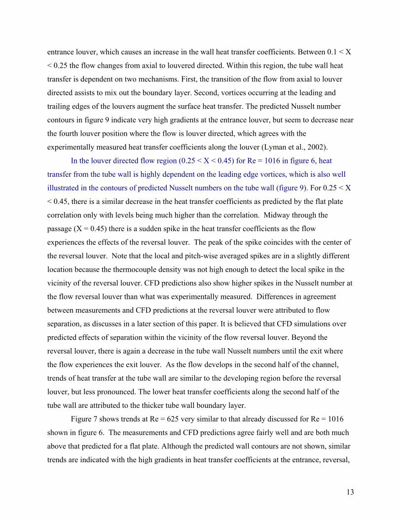
entrance louver, which causes an increase in the wall heat transfer coefficients. Between 0.1 < X
< 0.25 the flow changes from axial to louvered directed. Within this region, the tube wall heat
transfer is dependent on two mechanisms. First, the transition of the flow from axial to louver
directed assists to mix out the boundary layer. Second, vortices occurring at the leading and
trailing edges of the louvers augment the surface heat transfer. The predicted Nusselt number
contours in figure 9 indicate very high gradients at the entrance louver, but seem to decrease near
the fourth louver position where the flow is louver directed, which agrees with the
experimentally measured heat transfer coefficients along the louver (Lyman et al., 2002).
In the louver directed flow region (0.25 < X < 0.45) for Re = 1016 in figure 6, heat
transfer from the tube wall is highly dependent on the leading edge vortices, which is also well
illustrated in the contours of predicted Nusselt numbers on the tube wall (figure 9). For 0.25 < X
< 0.45, there is a similar decrease in the heat transfer coefficients as predicted by the flat plate
correlation only with levels being much higher than the correlation. Midway through the
passage (X = 0.45) there is a sudden spike in the heat transfer coefficients as the flow
experiences the effects of the reversal louver. The peak of the spike coincides with the center of
the reversal louver. Note that the local and pitch-wise averaged spikes are in a slightly different
location because the thermocouple density was not high enough to detect the local spike in the
vicinity of the reversal louver. CFD predictions also show higher spikes in the Nusselt number at
the flow reversal louver than what was experimentally measured. Differences in agreement
between measurements and CFD predictions at the reversal louver were attributed to flow
separation, as discusses in a later section of this paper. It is believed that CFD simulations over
predicted effects of separation within the vicinity of the flow reversal louver. Beyond the
reversal louver, there is again a decrease in the tube wall Nusselt numbers until the exit where
the flow experiences the exit louver. As the flow develops in the second half of the channel,
trends of heat transfer at the tube wall are similar to the developing region before the reversal
louver, but less pronounced. The lower heat transfer coefficients along the second half of the
tube wall are attributed to the thicker tube wall boundary layer.
Figure 7 shows trends at Re = 625 very similar to that already discussed for Re = 1016
shown in figure 6. The measurements and CFD predictions agree fairly well and are both much
above that predicted for a flat plate. Although the predicted wall contours are not shown, similar
trends are indicated with the high gradients in heat transfer coefficients at the entrance, reversal,

14
and exit louvers. The predictions indicate that by the fourth louver, the heat transfer contours
indicate a repeating pattern and as such indicates that the flow is once again louver directed. As
one would expect, the primary difference between figures 6-8 are the occurrence of lower heat
transfer coefficients at the lower Reynolds number.
4.2 Augmentation of the Tube Wall Heat Transfer The augmentation of the tube wall heat transfer coefficients can be calculated relative to
the heat transfer coefficients for a flat plate and relative to the heat transfer coefficients occurring
along each individual louver. Figure 10 shows the augmentation of the tube wall heat transfer
coefficients relative to that occurring along a flat plate at Re = 230, 625, and 1016. As can be
expected from the presence of additional secondary flow motions, which will be discussed in the
next section, there is a definite enhancement of the heat transfer coefficients relative to what
would occur for a flat plate with values ranging between 1 and 2 over most of the tube wall
surface.
Figure 11 compares the ratio of the heat transfer coefficients along the tube wall to that of
the heat transfer coefficients occurring along each individual louver. Note that spatially resolved
heat transfer coefficients were previously reported by Lyman et al. (2002) along the louver for
the same Reynolds number and geometry. These heat transfer coefficients were spatially-
averaged along each of the louver surfaces (from louver 2 to 8). The averaged Nusselt numbers
for each louver were then used in the denominator of the augmentation ratio, as shown in figure
11. Since data regarding the heat transfer coefficients are unavailable for Re = 625, only
augmentation ratios for Re = 230 and 1016 are shown in figure 11. Note that the louver heat
transfer coefficients used the local bulk temperature as the reference temperature, which is more
relevant for the louvers since the bulk temperature takes into account the added heat from the
upstream louvers. The results indicate that the heat transfer coefficients are much lower on the
tube wall than along the louver surfaces, which is most likely a result of the boundary layer
beginning at the start of each louver in contrast to a more continuous boundary layer along the
tube wall. Within the vicinity of (0.3 < X < 0.45), where the flow is louver directed, the ratio of
tube wall to louver heat transfer is approximately 0.4 for Re = 1016 and 0.3 for Re = 230. These
values are almost double the predicted values reported by Tafti and Cui (2003) in the louver
directed region. The differences between our study and that of Tafti and Cui (2003) can mainly
15
be attributed to the following: First, Tafti and Cui (2003) heated both the tube wall and the
louvers; thus surrounded the tube wall with a warmer thermal field than in this study. Second, the
developing flowfield and heat transfer effects at the entrance, reversal, and exit louvers are
included in our study, whereas Tafti and Cui (2003) considered only fully developed flow.
Although it is not presented here, the velocity and thermal boundary layer thicknesses
were calculated from the CFD predictions along the tube wall in number of axial locations and
compared with what would be expected for a flat plate boundary layer. The thicknesses in the
pitch wise center of the louvers were found to be significantly thinner than that expected from
flat plate correlations. As an example, consider the fifth louver where the boundary layer
thickness was 13% of the louver pitch, as compared with that predicted for a flat plate, which
was 31% of the louver pitch.
4.3 Thermal Fields Along the Tube Wall With the intention of understanding the effects augmenting the tube wall heat transfer, an
analysis was completed of the predicted thermal fields in various locations along the louver
array. These thermal fields were analyzed at the key locations shown in figure 12 as P1 through
P5 for Re = 1016. Note that these planes were placed normal to the tube wall surface where the
local coordinates are defined as (x΄,y΄,z΄) . The thermal fields shown in figures 13 – 15 are
presented in terms of a non-dimensional temperature, θ, which is based on the inlet temperature
and the local wall temperature. θ is given by equation 3 as
inw
in
TTTT
−−
=θ (3)
Note wT was calculated along the thermal field of interest.
Figures 13 – 15 show the thermal fields, resulting from the complicated flow structures
along the tube wall, as analyzed on planes P1 through P5. Starting with P1, the thermal field
between louver 1 (shown as the black vertical bar at y = 0.3) and the entrance louver (shown as
dotted lines at y = 0.7) is shown in figure 13. A fairly consistent and thin thermal field exists on
both sides of the first louver. As one moves past the first louver on the y-axis the thermal field

16
suddenly thickens, particularly in the region of (0.5 < y < 0.7). This phenomenon can be
attributed to two effects. First, as the axial directed flow approaches bend in the entrance louver,
it no longer remains attached to the entrance louver and separates. Second, as the flow passes the
entrance louver, a wake is produced. It is believed that both of these phenomena thicken the
thermal fields within the (0.5 < y < 0.7) region as illustrated in figure 13. This thickening of the
boundary layer causes high gradients in the heat transfer coefficient as illustrated in figure 9.
As mentioned earlier, it is suspected that leading edges of the louvers help augment heat
transfer along the tube wall. This effect is apparent from figures 6 – 8 as well as in the contour
plot of the tube wall Nusselt number shown in figure 9. To better understand the mechanism that
augments heat transfer at the leading edges, thermal fields at locations P2 and P3 were created.
From figure 14a, it is obvious that as the flow approaches the leading edge of louver 5, a vortex
is created and the surrounding thermal field is thinned. As shown in figure 14a, the thermal field
is considerably uniform from (-0.3 < x < -0.1) until approximately x = -0.09, where there is a
significant downturning of cooler fluid towards the wall. The leading edge vortex causes a
sudden decrease in θ and is the mechanism responsible for high Nusselt numbers at the leading
edges of all the louvers in figure 9. In addition to augmentation at the leading edge, the
downwash caused by the leading edge vortex also augments heat transfer along the louver pitch.
So strong are the effects of the leading edge vortex, that boundary layer thinning is still evident
in figure 14b (0.1 < y < 0.5), of which P3 is located 30% of a louver pitch upstream of the
leading edge. Figure 9 shows the augmentation along the louver pitch due to the downwash of
cooler fluid by the leading edge vortex. The wake of the trailing edge of louver 4 (represented by
dotted lines) is also well illustrated in figure 14b within (0.62 < y < 0.76) where the thermal field
is slightly extended. Since the increase in the thickness of the thermal boundary layer is only
slightly increased within this region there is not a dramatic decrease in Nusselt number at the
trailing edges of the louvers as shown in figure 9.
Comparable to the separation effects occurring within the vicinity of the entrance louver
are the flow structures resulting from the flow reversal louver. For the case of the reversal louver,
separation and the extension of the surrounding thermal fields are more pronounced than at the
entrance louver. The larger separation was expected since the flow reversal louver imposes a 54o
change rather than 27o change to the flow path as imposed by the entrance louver. Extension of
the thermal field is well illustrated in the contours of θ shown in figures 15a-b. As shown in

17
figure 15a, the underside of the flow reversal louver (-0.32 < Y΄/Lp< 0) serves to thin the thermal
boundary layer, whereas along the top surface of the reversal louver, the thermal boundary layer
is extended. Since the strongest effect of separation was expected to occur at the final bend of the
flow reversal louver, plane P5 (figure 15b) was used to capture any separation affects that might
occur. Figure 15b, clearly shows that before the solid vertical bar (representing reversal louver),
the thermal boundary layer thickness is thin (0 < y < 0.2). θ also becomes smaller as the louver is
approached. However, on the opposite side of the vertical bar (0.3 < y < 0.84), the thermal
boundary layer is extended. The larger values of θ, which result from a thicker thermal field, are
comparable to that of the entrance louver.
5. CONCLUSIONS
In this paper, experimental and computational results of the heat transfer at the tube-fin
junction for louvered fin heat exchangers have been presented. Commonly used as a method to
increase fin heat transfer, it has been determined that louvered fins also augment tube wall heat
transfer. For all Reynolds numbers investigated, reasonable agreement with steady, three-
dimensional computational predictions where achieved. Through thorough experimental
measurements and computational predictions, it has been determined that an augmentation ratio
of up to 3 times can occur for a tube wall with fins as compared to a flat plate. Secondary flow
patterns caused by vortices and separation were defined as the mechanisms that augment tube
wall heat transfer. Vortices near the leading edge of the louvers have been determined to increase
heat transfer by thinning the tube wall boundary layer. While the entrance and reversal louver
cause separation, it has been determine that these louvers are vital in re-starting the boundary
layer for the tube wall located downstream of them.
Acknowledgments
The authors gratefully acknowledge Modine Manufacturing Company for sponsoring the work that was presented in this paper.

18
Nomenclature A Louver surface area Ac,f Cross sectional area of a straight fin Fp Fin pitch h Convective heat transfer coefficient, )TT(qh inw
" −= Average heat transfer coefficient of the first louver (Lyman, et al. 2002)
kf Thermal conductivity of the balsa wood Lp Louver pitch, length of louver Lf Length of the fin Nu Nusselt number based on louver pitch, Nu = h Lp / k NuL Average Nusselt numbers of louvers 2-8 (Lyman, et al.) Nuo Baseline Nusselt number given by the flat plate correlation, equation 2 (Incropera and DeWitt, 1996) Pf Perimeter of a straight fin Applied heat flux boundary condition Convective heat flux from heated wall Heat flux lost due to conduction Heat flux lost due to radiation Re Reynolds number based on louver pitch, Re = Uin·Lp/ν Rp Resistance of the precision resistor Rc Thermal resistance between the conduction guard heater and the tube wall t Louver thickness Tw Surface temperature of the tube wall TP1 Surface temperature of the conduction guard heater TP2 Surface temperature of the radiation guard heater Uin Inlet face velocity to test section X΄,Y΄,Z΄ Fin dimensional coordinate system, see figure 1 X,Y,Z Normalized fin dimensions, (X΄/Lf , Y΄/Lf, Z΄/Lf) x΄,y΄z΄ Louver dimensional coordinate system, see figure 11 x,y,z Normalized louver dimensions, (x΄/Lp , y΄/ Lp, z΄/Lp) Greek θ Louver angle, non-dimensional temperature (see equation 3) ν Kinematic viscosity
Lχ Fraction of tube wall-louver radiation losses to applied heat flux (as given by RTE)
Wχ Fraction of tube wall-lexan wall radiation losses to applied heat flux
Lε Emissivity of the louvers
wε Emissivity of the milled lexan wall σ Stefan-Boltzmann constant ∆T Temperature difference between strip 1 and the inlet air
fη Effectiveness for an infinitely long fin (Incropera and DeWitt, 1996)
"q
"rq
"powerq
"cq
fh
19
Superscripts ¯ Averaged value ΄ Dimensional values
References Achachia, A., Cowell, T. A. 1988. Heat Transfer and Pressure Drop Characteristics of Flat Tube and Louvered Plate Fin Surfaces. Experimental Thermal and Fluid Science. 1: 147-157. Atkinson, K. N., Drakulic, R., Heikal, M. R., Cowell, T. A. 1998. Two and Three dimensional Numerical Models of Flow and Heat Transfer Over Louvred Fin Arrays in Compact Heat Exchangers. International Journal of Heat and Mass Transfer. 41: 4063- 4080. Beauvais, F. N. 1965. An Aerodynamic Look at Automobile Radiators. SAE 650470. Davenport, C.J. 1983. Correlations for Heat Transfer and Flow Friction Characteristics of Louvered Fin Heat Transfer. AICHE Symposium Series. 79: 19-27. FLUENT/UNS User’s Guide. 2002. Release 6.1. Fluent Inc., Lebanon, New Hampshire. Incropera, F.P. and DeWitt, D.P. 1996. Fundamentals of Heat and Mass Transfer. pp.120-122, 352, 358. New York: Wiley. Kays, W. M. and London, A.L. 1984. Compact Heat Exchangers. pp. 1-75. New York: McGraw-Hill. Kline, S.J. and McClintock, F.A. 1953. Describing Uncertainties in Single Sample Experiments. Mech. Engineering. pp. 3-8. Lyman, A. C., Stephan, R. A., Thole, K. A., Zhang, L., Memory, S. 2002. Scaling of Heat Transfer Coefficients Along Louvered Fins. Experimental Thermal Fluid Science. 26 (5): 547-563. Lyman, A. 2000. Spatially Resolved Heat Transfer Studies in Louvered Fins for Compact Heat Exchangers, MSME Thesis.Virginia Tech, USA.
Moffat, R. J. 1988. What’s New in Convective Heat Transfer? International Journal of Heat and Fluid Flow. 19: 90-101. Namai, K., Muramoto, H., Mochizuki, S. 1988. Flow Visualization in the Louvered Fin Heat Exchanger. SAE 980055.

20
Siegel, R. and Howell, J. 1981. Thermal Radiation Heat Transfer. pp. 833-837. New York: HPC.
Springer, M. E., K.A. Thole. 1998. Experimental Design for Flowfield Studies of Louvered Fins. Experimental Thermal and Fluid Science. 18: 258-269. Tafti, D.K., Zhang, L.W., Huang, W., Wang, G. 2000. Large-Eddy Simulations of Flow and HeatTransfer in Complex Three-Dimensional Multilouvered Fins. ASME Fluids Engineering Division Summer Meeting. FEDSM2000-11325. Boston, Massachusetts, 11 15 June. Tafti, D.K. and Cui, J. 2002. Computations of flow and heat transfer in a three dimensional multilouvered fin geometry. International Journal of Heat and Fluid Flow. 45: 5007-5023. Tafti, D.K. and Cui, J. 2003. Fin-tube junction effects on flow and heat transfer in flat tube multilouvered heat exchangers. International Journal of Heat and Fluid Flow. 46: 2027-2038. Webb, R. L.,Trauger, P. 1991. Flow Structure in the Louvered Fin Heat Exchanger Geometry. Experimental Thermal and Fluid Science. 4: 205-214.

21
TABLE 1. Summary of Louvered Fin Geometry
Louver Angle (θ) 27˚ Fin Pitch to Louver Pitch (Fp/Lp) 0.76 Fin Thickness to Louver Pitch (t/Lp) 0.08 Number of Louvers 17 Channel depth to Louver Pitch (d/Lp) 6.3 Scale factor for testing 20
Exit Louver
Entrance Louver Note: Z΄-direction is normal to page
Fin Pitch (Fp)
Louver Pitch (Lp)
Inlet Face Velocity, Uin
Louver Angle (θ)
θ Y΄
X΄
Reversal Louver
Z΄
Tube-fin junction
FIGURE 1. Typical louvered-fin compact heat exchanger: (a) assembly and (b) side view of louvered fins.

22
FIGURE 2. Schematic of flow facility for the louvered fin tests.
Aluminum plate
Radiation guard heaters
Milled lexan wall
Instrumented heated wall (as shown in figure. 4)
Conduction guard heaters
FIGURE 3. Schematic of the test section components.
Tp1
Tp2
23
Top thermocouple
Heater strips Copper bus bars
Center thermocouple
Power leads
Bottom thermocouple
FIGURE 4. Wiring diagram and thermocouple map of heat transfer surface.
0
2
4
6
8
10
-0.2
0
0.2
0.4
0.6
0.8
1
0 0.25 0.5 0.75 1
Nu, ∆T = 9 oC
Nu, ∆T = 15 oC
χL, ∆T = 9oC
χL, ∆T = 15 oC
χW
, ∆T = 9 oC
χW
, ∆T = 15 oC
Nuχ
W
χL
X
FIGURE 5. Experimental measurements of the tube wall Nusselt number and predictions
of χw and χL as a function of ∆T for Re = 230.
24
0
5
10
15
20
25
0 0.2 0.4 0.6 0.8 1
CFD, localCenterBottom
Top
Flat Plate, equation 2CFD, Pitch-wise average
Nu
X
FIGURE 6. Measurements and CFD predictions of Nusselt numbers along the tube wall
compared to the flat plate correlation for Re = 1016.
0
5
10
15
20
25
0 0.2 0.4 0.6 0.8 1
CFD, localCenterBottom
Top
Flat Plate, equation 2CFD, Pitch-wise average
Nu
X
FIGURE 7. Measurements and CFD predictions of Nusselt numbers along the tube wall
compared to the flat plate correlation for Re = 625.

25
0
3
6
9
12
15
0 0.2 0.4 0.6 0.8 1
CenterCFD, localTop
Bottom Flat Plate, equation 2CFD, Pitch-wise average
Nu
X
FIGURE 8. Measurements and CFD predictions of Nusselt numbers along the tube wall
compared to the flat plate correlation for Re = 230.
1 2 4 6 8 10 12 14 16 18 20
FIGURE 9. CFD contours of Nusselt numbers along the tube wall for Re = 1016.
Nu

26
1
1.5
2
2.5
3
3.5
4
0 0.2 0.4 0.6 0.8 1
exp, Re = 230
CFD, Re = 230exp, Re = 1016
CFD, Re = 1016exp, Re = 625 CFD, Re = 625
Nu / Nuo
X
FIGURE 10. Augmentation ratio of the tube-wall as compared to that of the flat plate correlation.
FIGURE 11. Augmentation ratio of the tube-wall as compared to the average louver heat transfer coefficient.
0.2
0.3
0.4
0.5
0.6
0.7
0.8
0.9
1
0.1 0.15 0.2 0.25 0.3 0.35 0.4 0.45
CFD, Re = 1016
exp, Re = 1016
CFD, Re = 230
exp, Re = 230
Nu / NuL
X

27
FIGURE 12. Locations of thermal field planes that were analyzed.
P1 P2 P3 P4 P5
x΄ y΄ z΄
z
y
θ
0 0.1 0.2 0.3 0.4 0.5 0.6 0.7 0.80
0.1
0.2
0.3
0.4
0.5 1.61.51.41.31.11.00.90.80.70.60.50.30.20.10.0
FIGURE 13. Thermal field for plane P1, Re = 1016.

28
a) Plane P2
b) Plane P3
y
z
θ
0 0.1 0.2 0.3 0.4 0.5 0.6 0.7 0.80
0.1
0.2
0.3
0.4
0.5 1.61.51.41.31.11.00.90.80.70.60.50.30.20.10.0
θ
1.61.51.41.31.11.00.90.80.70.60.50.30.20.10.0
z
x
-0.3 -0.2 -0.1 00
0.1
0.2
0.3
0.4
0.5
FIGURES 14a-b. Thermal fields for planes P2 and P3, Re = 1016.

29
a) Plane P4
b) Plane P5
FIGURES 15a-b. Thermal fields for planes P4 and P5, Re = 1016.
z
Y΄/Lp -0.3 -0.2 -0.1 0 0.1 0.2 0.3
0
0.1
0.2
0.3
0.4
0.5 1.61.51.41.31.11.00.90.80.70.60.50.30.20.10.0
θ
1.61.51.41.31.11.00.90.80.70.60.50.30.20.10.0
z
θ
y
0 0.1 0.2 0.3 0.4 0.5 0.6 0.7 0.80
0.1
0.2
0.3
0.4
0.5