child education and the family income gradient in china · child education and the family income...

1

Child Education and the Family Income Gradient in China

Luo Chuliang*, Paul Frijters**, and Xin Meng***

* Beijing Normal University, China

**School of Economics and Finance, University of Queensland, Brisbane, Australia

*** RSSS, Australian National University, Canberra, Australia

Abstract

This paper looks at the relation between education and family income using a 2008-2009

survey of nearly 10,000 children in 15 cities and nine provinces throughout China. We use

school test scores on mathematics and language, as well as parent-reported educational

progress, out-of-pocket expenses, and self-reported quality of schooling. Across all measures,

children from wealthier families do better, but the gap is much smaller for older children than

younger children in rural areas and is almost entirely gone at the end of secondary school. In

Chinese cities and in Western countries like the US the opposite is the case, with the gap

between children from poor and rich households staying constant or even widening as the

kids get older. Our explanation is that it takes a generation of universal education for ability,

education, and parental income to become highly correlated, which will already have

happened in Chinese cities and in Western countries, but is only just now happening in rural

areas in China. Accordingly, the relation between family income and child ability increases

over generations, reducing future education and income mobility.

2

1. Introduction

Nearly all developed and developing countries provide some state-funded

education for all children. Even though most systems have an explicit philosophy of

providing a level playing field for children, it remains the case that children of rich

families have better educational outcomes (Masters, 1969; Heckman, 2007; Cunha

and Heckman, 2008a, 2008b; Blanden and Gregg, 2004; Nam and Huang, 2009). In

Canada, for instance, 50.2% of youth from the families in the top quartile of the

income distribution attend university, whilst only 31% of youth from the bottom

quartile do so (Frenett, 2004). In the US, students‟ average SAT scores in

Mathematics and English increase by about 10 points for every extra $10,000 in

family income (Devine-Eller, 2004). Yet, the degree to which income and education

are related is not the same across countries, nor is it constant over time (Corak et al.,

2004; Loken, 2010). In terms of cross-country differences, Kaufmann (2008) reports

that only 4% of the student body in Brazil comes from the poorest 40% of the

population, whilst 20% of US students come from the poorest 40%. In terms of the

changing effect of income over time, Belley and Lochner (2007) find family income

played much less of a role in college attendance by comparing the 1979 and 1997

data from the NLSY. The differences across countries and time raise the question of

whether an education system can widen initial differences in educational attainment or

reduce them. Closely connected to this is the question of whether the differences in

outcomes are due to the children of richer parents having greater ability or more

opportunity.

In this mainly descriptive paper we look at the income-education relation for

China, which has had universal primary and secondary education in the cities for

about a generation, but has only recently seen universal education introduced in the

country side, where two-thirds of the population lives. Given this „first generation‟ of

educational streaming for the majority of the population, we are particularly interested

in whether the relation between income and education outcomes becomes stronger or

weaker as the child is at school for longer. Reasons an education system might

3

aggravate initial differences that are often cited are credit constraints or differential

school quality across socioeconomic regions (Carneiro and Heckman, 2002; Keane,

2002; Li, 2007; Frenette, 2007). Since school education is locally funded in China,

education quality co-moves with the wealth of neighbourhoods, and our data also

shows rich families buy additional tuition time for their children. This would lead

one to expect an increasing relation between income and education as the child ages.

On the other hand, in a first-generation system, family income and child ability are

likely to be less related to each other than they would be in a more established

education system, where several generations have gone through education and where

incomes are decided by a labour market that strongly rewards education. In a first

generation scenario, one would expect the richer families to still try to give their

children all the advantages they can, but for the more able children from poorer

families to catch up during their school years and thus for the gap between poor and

rich children to narrow as the children age. What makes the Chinese case

particularly interesting is that the urban education system is in its second generation.

If there is less convergence, or even divergence, of educational outcomes across

income groups as children get older in the cities, then that would indicate the

income-education relation is largely driven by the link between the ability of children

and their parental income. This is important for policy because if educational

outcomes are mainly ability-generated then the potential role of childhood

interventions to reduce later-life inequality via education is going to be limited at best.

We use a recent Chinese data set that covers 15 provinces and includes an array of

educational outcomes across the age range. Our chief measure of educational outcome

is the result of grade-standardised cognitive school tests that are given to children at

the end of each school semester in mathematics and language. Heckman (2007) and

Cunha and Heckman (2008a, 2008b) reported on a similar measure for the NLSY in

the US (the PIAT scores) and found that for the US, mathematics scores were higher

for children from wealthier families, and this relationship strengthened over time

(though maternal education significantly reduced the gradient, just as with health)-

4

what does „just as with health‟ refer to? Maternal education?. One of our chief aims is

to see whether the same is true in China. In addition to test-scores, we use

parent-reported school quality, parent-reported total family expenses on education,

and parent-assessed school evaluations.

In Section 2, we briefly discuss the educational institutions in China, and a

descriptive model of the relation between income and child ability that highlights the

interplay between the ability of the child, school outcomes, parental ability, and

parental income. Our data set is introduced in Section 3. In Section 4 we analyse the

child education-income relation with particular regard for the differences between the

country-side and the cities. Section 5 concludes.

2. Institutional background and a descriptive model

2.1 Educational institutions and their reforms

Education has traditionally been seen as important in Chinese society, partially

because national exams that gave access to desirable civil service jobs had been

institutionalised for centuries. The communist party took this system away in the early

1950s, but re-introduced it in the 1990s. The communist period also witnessed a very

modest relation between education and income: in the Mao era of the planned

economic regime (1949-1977), wages were administratively determined and rates of

return to education were very low. Since the economic reforms the importance of

education for income has increased rapidly, with rates of return estimated to be only 4%

in 1988 but 10.2% in 2001 (Zhang et al., 2005; Zhang et al. 2002; Li, 2003).

Though the link between education and income was weak before the 1990s, the

education system has expanded rapidly ever since the communist takeover in 1949.

Figures 1 to 3 show the increase over time in completion rates for junior high school

(which entails about 9 years of schooling) and senior high school (12 years). The data

comes from the 1986 and 2000 censuses and differentiates the subjects by age and

urban/rural divide. The main points of Figure 1-3 are that completion rates have

5

increased steadily since the 1920s, and there is a strong rural-urban divide: there was

almost a 100% completion rate of junior high school in the cities already in the 1960s

whereas, in the countryside, completion rates have only reached 80% during the

current generation.

Three dates stand out in these graphs, connected with particularly important

reforms. The first denotes the start of the communist era (1949), first affecting the

junior high school completion rates of the cohorts born after 1935. The second key

date is the end of the Mao era in 1977, with the last cohort finishing junior high under

that system being born in 1963. The third date is 1986 which is when the government

implemented the 9 Year Compulsory School Law, which aimed for 100% enrollment

at junior high school.

Figure 1 shows the big increase in completion rates throughout China during the

initial decades of the communist era. Figure 2 shows that during the pre-Mao era,

male junior high school completion rates were about 40% lower in the rural country

side than in the cities, and were still 20% lower at the end of the Mao era, whilst they

converged to within 10% for the last cohort to have finished junior high school at the

time of the 2000 census. For females, the differences between the country side and the

cities were bigger, with an almost 50% difference before the Mao era, with still nearly

40% fewer completions in the country side at the end of the Mao era, and still being

15% behind the urban completions for that period.. It is interesting to note that even

during the period of the Cultural Revolution (1966-1976) when schools were closed

and large groups of urban children were sent to the country side, the proportion of

urban males and females who completed junior high school nevertheless increased to

above 80%.1

One of the reforms at the end of the Mao era was a decentralisation which

involved the dissolution of local communes and a redistribution of land to individual

households. As rural teachers were paid by communes during the Mao era, the

1 For the urban population the cohorts born between 1953 to 1955 were given junior high school certificates

even though they did not actually spend much time at junior high school due to the school closing at the beginning of the Cultural Revolution (see Meng and Gregory, 2002).

6

dissolution of the communes had a detrimental effect on rural education because there

wasn‟t a clear system to take over the role of the communes in education. Figure 2

shows how the proportion of the rural population finishing junior high school dipped

for those who were born after 1963 and were enrolled in junior high schools after the

economic reforms. The trough immediately after this reform is even deeper than that

generated by the Cultural Revolution.

Following the 9 Year Compulsory School Law, individuals who were born in

1974 or later saw a considerable increase in the junior high school completion rate,

which also reduced the inequality in completion rates between the cities and the

countryside.

Beyond junior high school, however, the rural-urban divide has not improved

until recently. Figure 3 shows that, for the last cohort in the 2000 census (those who

were born in 1980), the urban male and female populations both had an above

80%completion rate for senior high school, whereas this rate was below 20% for

males and females in the rural area. As we will see with our own data from 2008-2009,

there has been a huge increase in the enrolment rates in the country side in the last 10

years, but the gap between rural and urban rates is still significant.

Equality in enrollment is only one of the measures of educational inequality.

Education quality is another aspect affected by the various reforms. An important

reform occurred to the administration and finance of education, which were

decentralised to the local level in the 1980s, and further privatised in the 1990s. As a

result, the quality and access to different qualities of schooling differs between cities

and the countryside and between rich and poor students within cities and rural areas.

Given that urban wage rates are more than double those in the countryside (Meng et

al., 2010), the quality of schools in urban areas is much higher and there is a lot of

disparity in school quality throughout the system (Knight and Li, 1996; Tsang, 1996;

Hannum and Wang, 2006; Wu, 2010; Zhang and Kanbur, 2005). Richer parents can

hence buy access to better schools, buy more private tuition, and have less need after

school hours to use their children‟s time for income-generating activities (such as

7

farming). Add onto these factors the fact that recent decades have seen an increase in

income inequality, we have good a priori reasons to expect a strong effect of family

income on educational achievements in China.

In terms of the broad picture, the communist era was one with a great increase in

educational enrollments but where education mattered relatively little for family

incomes. Whilst the cities have witnessed near universal junior high school education

since the 1960s, this has only been true in the rural areas in the last generation.

8

2.2 A descriptive model of education, family income, and child ability

Our analytical framework for analysing the dynamics of education, income, and

ability is a simplified version of the framework of Cunha and Heckman (2008a, 2008b)

in that parental ability is presumed to be linked to parental incomes via the labour

market and child ability via genetics and investments. Instead of writing down an

optimisation problem that focuses on the optimal decisions of the parents, we take the

investment feedback from parents to children as given and instead take a reduced

approach that looks directly at how the educational outcome of the child would

change year by year.

Suppose the educational outcome of child i after t years of schooling is driven by

innate ability and parental investments, which itself is a direct function of parental

income:

(1)

Here, is a weighting function that decreases with the years of

schooling (t goes from 0 to T), conveying the idea that as a child goes to school for

longer, the investments of the parents and random errors start to matter less and the

innate ability of the child starts to matter more; ) denotes cumulative parental

investments as a fraction of family income, and we interpret it to capture both

material resources (tuition and school quality) and immaterial resources (time after

school).

We think of the family income as itself related to the ability of the parents j which

is related via a genetic fraction ( ) to that of the child i:

(2)

(3)

where Educj refers to level of education of the parent, and is the fraction of

the household income related to parental ability. With and random elements

unrelated to ability and education, and with denoting the relative importance of

ability and education for family income ( denotes a rate of return).

9

These three equations allow for two effects of school expansion on the

relationship between parental income and children's school achievement. First, we can

think of the expansion of the education system as an increase in the total number of

years a child, i, is at school T. Because a higher T increases the importance of ability

in the final educational outcome (via w(t)), family income should start to matter less

as long as the relation between income and ability is not affected. The second-round

effect of a longer T though is to increase the correspondence between eventual income

and education (because education becomes a better measure of ability), which in turn

means that for the next generation, parental income becomes a better proxy for

parental ability. That second-round effect takes a generation though, meaning that in

the urban areas, children's innate ability should be more related to their parental

income than in the countryside.

If the relation between parental ability/education and their income further

increases because of increasing returns (an increase in ) then family income

becomes an even better proxy for parental ability. We can furthermore think of

behavioural effects, in that higher returns to education mean richer parents would

want to increase both T and their investments. The simplest way to think of this

behavioural effect is as a one-off increase in and hence as an increase in the

relation between family income and initial child education outcomes.

To see how these arguments can be empirically observed at the level of the child,

we consider the statistical relation between parental income and child educational

achievement over time2:

(4)

If we now look at whether this covariation increases or decreases as children go to 2 In most empirical applications, the variance of education is normalised over time, such as when age-standardised test scores are used. Given that the % of test-scores explained by income is typically modest (in our data all variables combined explain 10-20% of the standardised variance whilst income alone explains no more than 7%), the effect of the changes in the predictive ability of income on the standardised variation is very small.

10

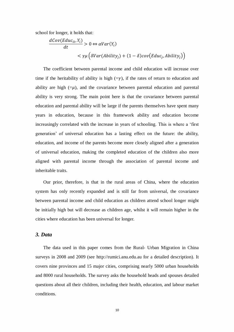
school for longer, it holds that:

The coefficient between parental income and child education will increase over

time if the heritability of ability is high (= ), if the rates of return to education and

ability are high (= ), and the covariance between parental education and parental

ability is very strong. The main point here is that the covariance between parental

education and parental ability will be large if the parents themselves have spent many

years in education, because in this framework ability and education become

increasingly correlated with the increase in years of schooling. This is where a „first

generation‟ of universal education has a lasting effect on the future: the ability,

education, and income of the parents become more closely aligned after a generation

of universal education, making the completed education of the children also more

aligned with parental income through the association of parental income and

inheritable traits.

Our prior, therefore, is that in the rural areas of China, where the education

system has only recently expanded and is still far from universal, the covariance

between parental income and child education as children attend school longer might

be initially high but will decrease as children age, whilst it will remain higher in the

cities where education has been universal for longer.

3. Data

The data used in this paper comes from the Rural- Urban Migration in China

surveys in 2008 and 2009 (see http://rumici.anu.edu.au for a detailed description). It

covers nine provinces and 15 major cities, comprising nearly 5000 urban households

and 8000 rural households. The survey asks the household heads and spouses detailed

questions about all their children, including their health, education, and labour market

conditions.

11

In 2009, household heads/spouses were asked about the test scores their children

received in the last end of semester tests that all children have to take on mathematics

and language. They were also asked to provide the full score for the exam so that the

researchers could derive consistent percentages of the test scores. The end of semester

tests are set by schools, based on national guidelines about curriculum content. Across

different regions, although the contents of the curriculum may be the same, the test

questions may differ. Because we are interested in relative mobility, we standardise

these tests by grade so that the standard deviation is 1 in all grades. By including

regional dummies, the variation we are relying on is the within-province variation.

These „objective‟ test scores are our main outcome measure.

Additionally, the household heads/spouses were asked to evaluate whether their

children‟s performance at school is „excellent‟, „good‟, „reasonable‟, or „poor‟. This

will be labeled as "subjective school performance" in the paper. Also, household

heads/spouses were asked to evaluate the relative quality of the school their children

were attending (labeled as "subjective school quality"), how much the household

spent on the private tuition of each child, and how much the household spent in total

on the education of each child.

We restricted the sample to families that have a household registration or „hukou‟

in the place they live and can thus send their children to the local school (i.e. we

exclude migrants who live in places where they do not have access rights to

education), and we select those families with kids in the age range of 6-14. For our

analyses of the objective test scores, we only use the 2009 data, though we use both

the 2008 and 2009 samples for other outcome variables which are available in both

waves. Our total sample for both years comprises 6647 children aged 6 to 14. Among

them 984 and 894 are urban children in 2008 and 2009, respectively; and 2428 and

2341 are rural children in the two years, respectively.

Our measure of income is standard, in that we use the (log of) per capita

household income from all sources, which is calculated by summing over an itemised

list of sources of income including imputed agricultural income. All incomes have

12

been deflated by regional PPP indictors (Brandt and Holtz, 2006)3 to allow for

comparisons across regions.

Table 1 shows descriptive statistics for all the variables used in the later

estimations, which include our different measures of educational outcomes,

demographics (age, gender and birth weight of the child and education and age of the

parents), school starting age of the child, and regional identifiers. On average,

children in our sample are around 11 years old and 55% of them are boys. The sex

ratio is slightly higher for our rural sample than for the urban sample. Children in the

urban areas start school at 6.4 years of age, while their counterparts in rural areas start

0.4 years later. Urban children have slightly higher birth weights (3.4kg) than their

rural counterparts (3.2kg).

As indicated in the last section, there is an education gap between rural and urban

parents. On average, 68 to 70% of urban fathers and 62 to 66% of urban mothers have

completed senior high or more. These ratios for rural parents, however, are as low as

16% (fathers) and 9% (mothers).

We find that the rural parents of our 6-14 year old children are on average aged

around 37-38, while their urban counterparts are between 38 and 40 years of age.

Thus, the “parent generation” in our sample was born around the 1970s, when rural

junior high or above completion rates were as low as 50-60 % whilst it was nearer 90%

for the urban region, although even there less than 60% of students completed senior

high school. This means that parental education and parental ability will probably

have been aligned more in the cities than in the countryside.

Figures 4(a) to 4(e) show the means of each of our educational outcomes by the

income decile of the households. The figures show a consistent and fairly monotonic

positive relation between higher education outcomes and income deciles, where one

has to bear in mind that the subjective outcomes of child performance and school

quality are reverse coded. Compared to the children of the lowest income decile, the

3 They computed the regional PPPs up to 2004. We extended their values to 2008-2009 using provincial CPI.

13

children of the highest income decile have a subjective educational outcome that is

about half a point lower (on a 1-4 scale); their subjective school quality is about .7

lower (on a 1-4 scale), and their language and mathematics scores are about 10%

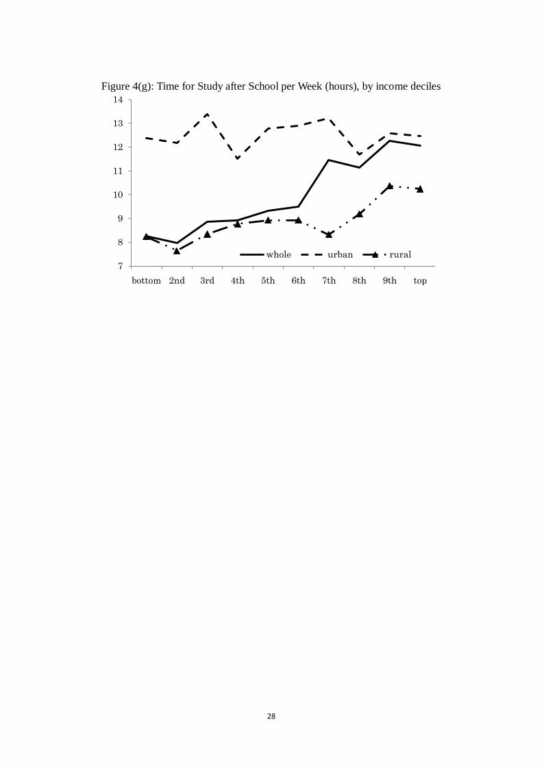
higher (nearly a standard deviation). Figures 4(f) and 4(g) show that the children from

richer households spend more time outside school on their education and have

significantly more resources spent on them, confirming that richer households indeed

try to help their children do well at school by having them spend more time on

education and allocating more resources towards them.

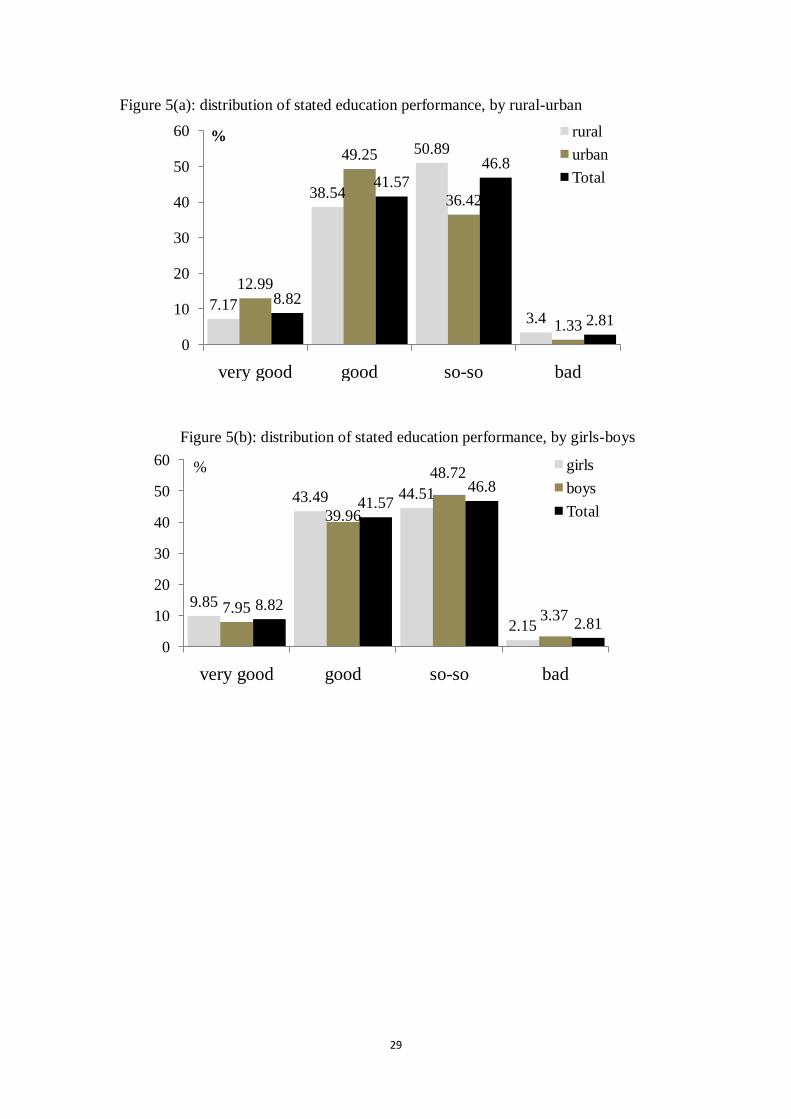
Figures 5(a) to 5(c) show the distribution of the two main subjective variables

(child schooling and school quality) by region and gender, revealing that school

quality is perceived to be much lower in the countryside, and that girls are thought to

do better than boys on average.

Finally, Figures 6(a) to 6(c) show measures of the income-education gradient for

children of different ages. Figure 6(a) shows that children of poorer households are

much more likely to prematurely end their education (before the age of 18) than

children of richer households, though it also shows that over 98% of the children are

still enrolled in school at age 14. Figure 3(a) also shows that secondary high school

attendance has increased significantly in the last 10 years. More than 90% of children

in the age-range 15-17 are still enrolled because at least two-thirds of the rural

children are still enrolled, even though the 2000 census shows only 10% completion

rates of secondary high school at that time. Figure 6(a) shows no significant selection

by income up to age of 14 (which is roughly grade 9), as less than 1% of the children

below 14 is not at school. Selection is very significant though for the 15-17 age group,

with children from poorer households much less likely to attend school than children

from richer households. For this reason, the 15-17 age group is dropped from the

subsequent graphs and analyses so that the results are not driven by selection.

Figure 6(b) and 6(c) show the relation between the normalised test scores by the

school grade for households above and below the medium incomes. Somewhat

surprisingly, and contrary to the results found with the NLSY in the US (Heckman,

14

2007), there is a clear reduction in the education-income relation over time. Whilst the

reduction in the last two grades will be somewhat driven by selection (only the

smarter kids of poorer households stay on in education), Tables 6(b) and 6(c) thereby

suggest a quite strong degree to which the initial differences in educational outcomes

reduce as children are in school for longer. Another way to put this is to say that the

initial advantage of having rich parents at age 6 wears off in China, whilst it has been

found not to wear off in the US.

Table 2 shows the correlation between our three separate measures of the

individual educational outcome of a child. Subjective Education Performance (SEP) is

surprisingly strongly correlated with both the language test scores and the

mathematics test scores of the children, with the Spearman Correlation terms 0.48 and

0.50 respectively. This gives some credence to the degree to which the results

attainable for SEP for the whole sample reflect the same relationship as that for the

more objective outcomes.

4. Analyses

Table 3 shows the results of our main regressions on the normalised test scores. In

the first column, we report only the raw direct relation, undifferentiated by age. In the

subsequent columns we differentiate by age and add more variables.

The results in the first and sixth columns show a strong effect of family income,

with a one-point increase in log family income leading to a 0.39 increase in language

tests (equivalent to 0.39 of a standard deviation) and a 0.38 increase in mathematics

tests. The results in columns two to five show that the income relationship becomes

weaker as more controls are added, but remains substantial and significant: the effect

of a one-point increase in log-income on language tests for a child aged 6 reduces

from 0.39 to 0.18 when we include information about the education of the parents,

birth weight, and region. The reduction is from 0.38 to 0.20 for mathematics tests.

15

Across these specifications, the income profile reduces with older children4. In

the fullest specifications in columns five and 10, the effect of family income for the

highest age range is about two-thirds of what it is for the youngest age range: for

language tests, the profile from youngest to oldest goes from 0.19 to 0.12, whilst the

profile for mathematics tests is from 0.20 to 0.11. The strong convergence is evidence

of a high degree of mobility within each school as to the relative ranking between

children, where the initial ranking is much more related to family income than the

eventual ranking.

Whilst we are primarily interested in the effect of income, the effects of the other

variables are quite logical. Boys do not perform as well in these tests, though the

difference in performance between genders is higher for language tests than

mathematical tests; children with higher educated parents do better, as do children

who weighed more at birth.

Extensions (i): region and gender

Table 4 shows the results for the Test Scores by region and gender. Due to the

lower number of individuals, there are some insignificant effects and revisions of the

initial profile. For the countryside, the overall pattern found for the whole country is

particularly pronounced for mathematics test scores, where the scores for the older

children are much less affected by income (0.086) than the younger children (0.174).

However this is not the case in the cities, where the oldest children are more affected

by family income than the youngest for both the language and mathematics tests. If

you like, Chinese cities look like the US in terms of an increasing income-education

profile as children age, whilst the country-side shows the opposite.

Another general finding from Table 4 is that on average, girls are more affected

by family income than boys. For the language tests for instance, girls aged 6 from

4 The results are qualitatively similar if we use linear interactions in stead of the two age-bands interacted with

income: in a specification with just income and age-income interactions, the interaction has a value of -0.025 (t-va; pf 2.9) , which would mean half the effect of income disappears after 9 years of schooling.

16

families with a one-point higher family income get 0.23 higher test-scores, whilst

boys get 0.16 higher test scores. A one-point increase in family income buys a 6-year

old a 0.15 increase language score in the countryside, whilst it only buys 0.05 in the

cities.

One of the potential explanations for why income matters more for girls than for

boys is the boy-preference in Chinese culture: the education of girls is more a residual

worry and thereby more likely to be important in high-income households than

low-income households.

One of the potential explanations for the higher gradient in the rural areas for

young children is that the importance of family income is likely to be stronger when

the region is not rich enough to provide high quality pre-school education. Income can

then buy access to private tuition and entry into better schools at the start of the

children‟s school career.

The differences between the rural and urban areas are consistent with the

observation that education has been important for much longer in urban areas than in

rural areas. In the countryside, the current cohort is the first generation to experience

universal education through to almost the age of 17. In the cities, this has been the

case for a generation longer. If we think that innate ability is the prime long-term

determinant of schooling outcomes and family income, this would mean that in the

cities, universal parental education has already fully sorted incomes and ability and

hence there is no convergence as children from different family incomes go through

school. In the countryside, there is high mobility as many children from poorer

families are more capable than their family income would indicate.

Extensions (ii):

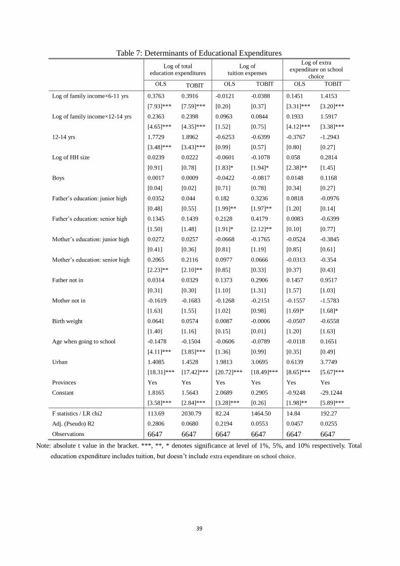
Tables 5 to 7 show the results for our other measures of educational outcomes, i.e.

the SEP, school quality, and family expenditures.

Columns one to five in Table 5 show the marginal effect of variables on the

17

probability of an „excellent‟ educational performance. A one-point increase in

log-income, for instance, increases the probability of an excellent educational

performance by 3.58%. This effect drops to 1.80% for 6-year olds when all the other

variables are included in column five. Since the results for the non-income factors are

almost a carbon-copy of those of the test scores, we further discuss only the general

points that arise for income.

In all the Tables 5 to 7, we get very similar results to Table 3: there is a strong and

significant relation between family income and education, but this relation reduces by

age. The one exception to this is in the last columns of Table 7 that show that

expenditures on particular schools are actually higher amongst the older children,

probably reflecting expenses of selective secondary schools. Yet, these expenses are

not high enough to counterbalance other expenses, so total expenses still become less

related to family income for older children.

What holds in all these analyses is that the estimated importance of income

reduces when additional controls are added, with a near halving of the effects once we

allow for parental education. A similar reduction in the explanatory power of

education was found for the US (Cunha et al. 2005, Cunha and Heckman 2008a;

Heckman 2007), but the reduction is weaker in China, strengthening our hypothesis

that parental education in China did not arise in a system of universal education and it

is thus possible that the lack of parental education is more related to the lack of

opportunities of the parents when they were young rather than their talents, unlike in

the US. We hence seem to be looking in China at the first generation that is

completely covered by education and where talent and education will strongly sort. As

a result, we should see in the future that the relation between income and education in

China becomes almost entirely driven by the relation between parental education and

child education, and we should see less convergence as children age than is the case

now.

18

5. Conclusions

This paper found that the relation between parental income and child education in

China is very strong for children just starting out in school, but reduces markedly as

children become older. Thus, the average test score of children in grade 10 (roughly

aged 16) is almost the same for families below median incomes and families above

median incomes. We find this reduction in profiles across age to be consistent for

different definitions of child education, including the quality of the school and

out-of-pocket expenses. The general conclusion is that the education system in China

works to reduce the importance of family income.

One of the potential reasons the results for China differ from those of the US,

where differences grow rather than reduce with age, is that there might be a „first

generation‟ effect of universal education in China. In the first generation, there is then

a free-for-all in which all families motivate their children to do well at school, which

is the recognised road to success. In that first generation, a high degree of mobility is

attained by able children whose parents were „unlucky‟ and hence have a low income.

After that first generation, ability and family income become more aligned and

mobility is less frequent. In such a situation, richer families still manage to give their

children a head start, which is very much in line with what we find in China when

richer children have more tuition fees spent on them and are stimulated to spend more

time on educational activities after school, but the head start gets eroded over the 12

years it takes to complete primary and secondary education.

Evidence for this hypothesis in our data is that the role of income reduces

markedly over time in the countryside where universal education is new but not for

children in urban areas, where it has existed for about a generation longer. It is also

consistent with the finding that parental education explains much less of the

income-child education relation in China than it does for the US.

An important element of the story is that the rates of return to education increased

in China in the last 30 years, leading both governments and households to be

19

interested in longer education and hence indirectly leading to a stronger sorting of

education and ability. Again, the analogy with the US is interesting because rates of

return have also increased in the US in the last 30 years, coinciding with an increased

relation between family income and college attendance (Belley and Lochner, 2007).

If this „first generation‟ hypothesis is true, we would expect that in future

generations in China, there would be a much closer relation between the wealth of the

parents and the education of the parents, in which case the percentage of children

from poorer families who manage to catch up would be much smaller because the

„innate‟ ability differences between children from rich and poorer households would

be higher and hence the relation would start to look a lot more like it does in the US.

The wider implications of the strong degree of educational mobility we now see

in China is that it is in principle possible for an education system to provide a road for

advancement to able children from a poor background. On the other hand, a „first

generation‟ general education system allows for a one-off sorting of education and

ability and would hence in general not lead to sustained high mobility in later

generations, which leads us to be rather pessimistic about the mobility potential of

children from poor backgrounds in countries with long-standing education systems.

20

References

Bainbridge, J., Meyers, M., Tanaka, S., and Waldfogel, J. (2005). Who Gets an Early

Education? Family Income and the Enrollment of 3- to 5-Year-Olds from 1968 to

2000. Social Science Quarterly, 86(3), 724-745.

Blanden, J., and Gregg, P. (2004). Family Income and Educational Attainment: A

Review of Approaches and Evidence for Britain. Oxford Review of Economic

Policy, 20(2), 245-263.

Belley, P., and Lochner, L. (2007). The Changing Role of Family Income and Ability

in Determining Educational Achievement. NBER working paper, No. 13527.

Brandt, L. & Holz, C.A. (2006). Spatial Price Differences in China: Estimates and

Implications. Economic Development and Cultural Change,55, 43-86.

Broaded M., and Liu, C. (1996). Family Background, Gender and Educational

Attainment in Urban China. China Quarterly, 145(March), 53-86.

Brown, P. (2006). Parental Education and Investment in Children‟s Human Capital in

Rural China. Economic Development and Culture Change, 54(4), 759-789.

Brown, P. H., and Park, A., (2002). Education and Poverty in Rural China. Economics

of Education Review, 21(6), 523-541.

Carneiro P., and Heckman, J. (2002). The Evidence on Credit Constraints in

Post-Secondary Schooling. Economic Journal, 112, 705-734.

Corak, M., Lipps, G., and Zhao, J. (2004). Family Income and Participation in

Post-Secondary Education. IZA Discussion Paper No. 977.

Cunha, F. and Heckman, J. (2008a). Formulating, identifying and estimating the

technology of cognitive and non-cognitive skill formation. Journal of Human

Resources, 43, 738-782.

Cunha, F., and Heckman, J. (2008b). A New Framework For The Analysis Of

Inequality. Macroeconomic Dynamics, 12(S2), 315-354.

Cunha, F., Heckman,J., Lochner, L., and Masterov, D. (2005). Interpreting the

Evidence on Life Cycle Skill Formation. NBER Working Papers 11331, National

Bureau of Economic Research.

Devine-Eller, A. (2004). Does Income Predict the Probability of College Entrance

Exam Preparation? Estimating Models with Logistic Regression. Retrieved from:

http://audreydevineeller.com/~auderey/Does%20Income%20Predict%20P%20of

%20Exam%20Coaching.pdf.

Ermisch J., and Francessconi, M. (2001). Family Matter, Impacts of Family

Background on Educational Attainments. Econonmica 68(270), 137-156.

Frenette, M. (2007). Why are youth from lower income families less likely to attend

university? Evidence from academic abilities, parental influences, and financial

constraints. Business and Labour Market Analysis, 2007(295), 1-39.

Hannum, E., and Wang, M. (2006). Geography and Educational Inequality in China,

China Economic Review, 17(3), 253-265.

Heckman, J. (2007). The economics, technology, and neuroscience of human

http://audreydevineeller.com/~auderey/Does%20Income%20Predict%20P%20of%20Exam%20Coaching.pdf

http://audreydevineeller.com/~auderey/Does%20Income%20Predict%20P%20of%20Exam%20Coaching.pdf

21

capability formation. Proceedings of the National Academy of Sciences, 104(33):

13250–55.

Kaufmann, K. M. (2008). Understanding the Income Gradient in College Attendance

in Mexico: the role of heterogeneity in expected returns to college. Department

of Economics, Stanford University.

Keane, M. P. (2002). Financial aid, borrowing constraints, and college attendance:

Evidence from structural estimates. American Economic Review, 92(2), 293-297.

Khanam, R., Hong Son Nghiem, H.S., and Connelly, L.B. (2009). Child Health and

the Income Gradient: Evidence from Australia. Journal of Health Economics, 28,

805-817.

Knight, J., and Li, S. (1996). Education Attainment and the Rural-Urban Divide in

China. Oxford Bulletin of Economics and Statistics, 58(1), 83-117.

Li, H., (2003). Economic Transition and Returns to Education in China. Economics of

Education Review, 22(3), 317-328.

Li, W. (2007). Family background, financial constraints, and higher education

attendance in China. Economics of Education Review, 26, 725-735.

Loken, K. V. (2010). Family Income and Children‟s Education: Using the Norwegian

Oil Boom as a Natural Experiment. Labour Economics, 17(1), 118-129.

Masters, S. H. (1969). The Effect of Family Income on Children‟s Education: Some

Findings on Inequality of Opportunity. Journal of Human Resources, 4(2),

158-175.

Meng, X. & Gregory, R. G. (2002). The Impact of Interrupted Education on

Subsequent Educational Attainment: A Cost of the Chinese Cultural Revolution,"

Economic Development and Cultural Change, University of Chicago Press,

50(4),935-59.

Name Y., and Huang, J. (2009). Equal Opportunity for All? Parental Economic

Resources and Children‟s Educational Attainment, Children and Youth Services

Review, 31(6), 625-634.

National Bureau of Statistics, China. (2009). Chinese Statistical Yearbook. n.p.:

Chinese Statistics Press.

Tsang, M. (1996). Financial Reform of Basic Education in China. Economics of

Education Review, 15(4), 423-444.

Wu, X. (2010). Economic Transition, School Expansion and Educational Inequality in

China, 1990-2000. Research in Social Stratification and Mobility, 28(1), 91-108.

Zhang, J., Zhang, Y., Park, A., and Song, X. (2005). Economic Return to Schooling in

Urban China, 1988 to 2001. Journal of Comparative Economies, 33(4), 730-752.

Zhang, L., Huang, J., and Rozelle, S. (2002). Employment, Emerging Labor Markets,

and the Role of Education in Rural China. China Economic Review, 13(2-3),

313-328.

Zhang, X., and Kanbur, R. (2005). Spatial Inequality in Education and Health Care in

Chin. China Economic Review, 16(2), 189-204.

Zhou, X., Moen, P., and Tuma N. B. (1998). Education Stratification in Urban China:

1949-1994. Sociology of Education, 71(3), 199-222.

22

Figure 1: 1982 census data: % completed junior high school

Note: the cohort born between 1961 and 1963 were aged 14-16 in 1977 (end of the Mao era)

and should be enrolled in Junior high school at that time.

0.2

.4.6

.81

% c

om

ple

ted jun

ior

hig

h s

ch

ool

1925 1930 1935 1940 1945 1950 1955 1960 1965byear

Rural Urban

Males

0.2

.4.6

.81

% c

om

ple

ted jun

ior

hig

h s

ch

ool

1925 1930 1935 1940 1945 1950 1955 1960 1965byear

Rural Urban

Females

23

Figure 2: 2000 census data: % completed junior high school

Note: the cohort born in 1963 is the last one going to school in the pre-reform period, while the

cohort finishing junior high in 1986 was born in 1974.

Figure 3: 2000 census data: % completed senior high school

0.2

.4.6

.81

% c

om

ple

ted jun

ior

hig

h s

ch

ool

1940194519501955196019651970197519801985byear

Rural Urban

Males

0.2

.4.6

.81

% c

om

ple

ted jun

ior

hig

h s

ch

ool

1940194519501955196019651970197519801985byear

Rural Urban

Females0

.2.4

.6.8

1

% c

om

ple

ted s

enio

r hig

h s

choo

l

1940 1945 1950 1955 1960 1965 1970 1975 1980birth year

Rural Urban

Males

0.2

.4.6

.81

% c

om

ple

ted s

enio

r hig

h s

choo

l

1940 1945 1950 1955 1960 1965 1970 1975 1980birth year

Rural Urban

Females

25

Figure 4(a): Evaluation on Education performance, by income deciles

Figure 4(b): Evaluation on school quality, by income deciles

2.1

2.15

2.2

2.25

2.3

2.35

2.4

2.45

2.5

2.55

2.6

bottom 2nd 3rd 4th 5th 6th 7th 8th 9th top

whole urban rural

2

2.1

2.2

2.3

2.4

2.5

2.6

2.7

2.8


whole urban rural

26

Figure 4(c): Language Test Scores, by income deciles

Figure 4(d): Mathematics Test Scores, by income deciles

77

79

81

83

85

87

89

91


whole urban rural

80

82

84

86

88

90

92

94


whole urban rural

27

Figure 4(e): Normalised Test Scores, by income deciles

Figure 4(f): Educational Expenditure (Yuan), by income deciles

-0.6

-0.4

-0.2

0

0.2

0.4

0.6

1 2 3 4 5 6 7 8 9 10

language mathematics

2

502

1,002

1,502

2,002

2,502tuition

total edcation expenditure

28

Figure 4(g): Time for Study after School per Week (hours), by income deciles

7

8

9

10

11

12

13

14


whole urban rural

29

Figure 5(a): distribution of stated education performance, by rural-urban

Figure 5(b): distribution of stated education performance, by girls-boys

7.17

38.54

50.89

3.4

12.99

49.25

36.42

1.33

8.82

41.57

46.8

2.81

0

10

20

30

40

50

60

very good good so-so bad

% rural

urban

Total

9.85

43.49 44.51

2.157.95

39.96

48.72

3.378.82

41.5746.8

2.81

0

10

20

30

40

50

60

very good good so-so bad

% girls

boys

Total

30

Figure 5(c): Distribution of reported school quality

3.96

23

70.69

2.35

13.26

54.15

32.16

0.436.59

31.8

59.8

1.81

0

10

20

30

40

50

60

70

80

excellent good general poor

% rural

urban

whole

31

Figure 6(a): Percentage of children not in School, by income deciles and age-groups

Figure 6(b): Normalised language scores by school grade for above and below

medium incomes.

0%

1%

2%

3%

4%

5%

6%

7%

8%

9%

10%


6-11 yrs 12-14 yrs

15-17 yrs whole sample

-0.5

-0.4

-0.3

-0.2

-0.1

0

0.1

0.2

0.3

0.4

1 2 3 4 5 6 7 8 9

normalised

scores

grades

< median > median

32

Figure 6(c): Normalised maths scores by school grade for above and below medium

incomes.

-0.5

-0.4

-0.3

-0.2

-0.1

0

0.1

0.2

0.3

0.4

0.5

1 2 3 4 5 6 7 8 9

normalised

scores

grades

< median > median

33

Table 1: Sample Description

Total

2008

urban

2008

rural

2009

urban

2009

rural

Outcome variables:

Subjective school performance: (1-excellent;

4-bad) 2.4361 2.2419 2.4815 2.2819 2.5297

Subjective school quality: (1-excellent; 4-bad) 2.5682 2.1768 2.6792 2.2204 2.7505

Objective test score (language, 100%) 83.6424

89.2766 81.4465

Objective test score (Math, 100%) 85.2888

90.5390 83.2236

Normalised test score (language) -0.0026

0.4770 -0.1895

Normalised test score (Math) -0.0003

0.4453 -0.1755

Log of family income per capita (Yuan) 8.4851 9.2193 8.1576 9.2653 8.2183

Age of the child (Years) 10.8523 10.6199 10.9320 10.5749 10.9731

Dummy for Boy 0.5448 0.5163 0.5564 0.5235 0.5528

Birth weight of the child (kg) 3.2573 3.3437 3.2176 3.3732 3.2178

Age start school 6.5578 6.3684 6.6219 6.3982 6.6318

Father‟s education: junior high 0.4313 0.1829 0.5391 0.1857 0.5177

Father‟s edu: senior high and above 0.3078 0.6707 0.1639 0.6957 0.1563

Mother‟s education: junior high 0.3869 0.2358 0.4588 0.2237 0.4383

Mother‟s edu: senior high and above 0.2419 0.6240 0.0865 0.6555 0.0846

Father's age 38.92 40.15 38.44 40.14 38.32

Mother's age 37.24 37.67 37.11 37.55 37.05

Father information is missing 0.1383 0.1057 0.1800 0.0906 0.1269

Mother information is missing 0.1432 0.0915 0.1767 0.0738 0.1568

Hebei 0.0370 0.0000 0.0523 0.0000 0.0508

Shanghai 0.0211 0.0783 0.0000 0.0705 0.0000

Jiangsu 0.1041 0.0874 0.1141 0.0917 0.1055

Zhejiang 0.0918 0.1016 0.0886 0.1085 0.0846

Anhui 0.1192 0.1138 0.1231 0.1186 0.1175

Henan 0.1586 0.1311 0.1647 0.1521 0.1662

Hubei 0.0733 0.0569 0.0778 0.0682 0.0773

Guangdong 0.2199 0.2490 0.2261 0.1913 0.2123

Chongqing 0.0552 0.0722 0.0465 0.0872 0.0449

Sichuan 0.1199 0.1098 0.1067 0.1119 0.1410

# of obs. 6647 984 2428 894 2341

34

Table 2: Correlation between Subjective Education Performance (SEP) and

Normalised Test Scores

Whole Urban Rural

Ordered

Probit OLS

Ordered

Probit OLS

Ordered

Probit OLS

Language -0.3355 -0.1605 -0.4485 -0.2119 -0.3201 -0.1519

[9.52]*** [9.38]*** [6.09]*** [5.67]*** [7.81]*** [7.81]***

Math -0.5319 -0.2398 -0.5812 -0.2671 -0.5204 -0.2313

[14.85]*** [14.26]*** [8.41]*** [7.88]*** [-12.31]*** [11.93]***

Constant 2.4537 2.4967 2.4542

[227.49]*** [100.53]*** [192.46]***

LR chi2 / F 1095.11 604.37 273.13 146.23 755.13 413.75

Pseudo / Adj R2 0.1791 0.2904 0.1568 0.2604 0.1758 0.2801

# of obs. 2949 2949 826 826 2123 2123

Spearman Correlation matrix

SEP Language SEP Language SEP Language

Language scores -0.4919 -0.4545 -0.4821

Math scores -0.5194 0.7675 -0.4831 0.6847 -0.5100 0.7632

Note: absolute z value (for ordered probit model) and t value (for OLS) in the bracket. ***, **, *

denotes significance at level of 1%, 5%, and 10% respectively.

35

Table 3: Estimated Gradients of Family Income on Normalised Test Scores in China

Test scores for Language Test scores for Math

(1) (2) (3) (4) (5) (6) (7) (8) (9) (10)

Log of family income 0.3924

0.3768

[17.57]***

[16.78]***

Log of family income×6-11 yrs

0.4153 0.232 0.1924 0.1884

0.4103 0.2415 0.2015 0.1978

[14.23]*** [6.77]*** [5.57]*** [5.47]***

[13.97]*** [6.89]*** [5.71]*** [5.61]***


0.3533 0.1715 0.1317 0.124

0.3221 0.1535 0.1159 0.1086

[10.19]*** [4.49]*** [3.44]*** [3.24]***

[9.24]*** [3.95]*** [2.98]*** [2.79]***

11-14 yrs

0.4335 0.4438 0.4498 0.4905

0.6581 0.6809 0.6659 0.705

[1.12] [1.18] [1.20] [1.31]

[1.69]* [1.78]* [1.75]* [1.86]*

Log of HH size

0.0118 0.0036 0.004

-0.0108 -0.0167 -0.0166

[0.87] [0.27] [0.29]

[0.77] [1.19] [1.18]

Boys

-0.1472 -0.1524 -0.1491

-0.0656 -0.0707 -0.0681

[4.36]*** [4.51]*** [4.42]***

[1.91]* [2.06]** [1.98]**

Father‟s education: junior high

-0.0879 -0.0832

-0.182 -0.1784

[1.71]* [1.63]

[3.46]*** [3.40]***

Father‟s education: senior high

0.0452 0.0439

-0.0738 -0.0757

[0.72] [0.70]

[1.15] [1.19]

Mother‟s education: junior high

0.1391 0.1408

0.1202 0.1216

[2.88]*** [2.92]***

[2.43]** [2.46]**

Mother‟s education: senior high

0.2688 0.2662

0.2983 0.2962

[4.01]*** [3.98]***

[4.38]*** [4.35]***

Father not in

-0.142 -0.1385

-0.1943 -0.1918

[2.01]** [1.96]**

[2.67]*** [2.64]***

Mother not in

-0.0599 -0.0501

-0.0474 -0.0386

[0.86] [0.72]

[0.65] [0.53]

Birth weight

0.0322 0.0297

0.0488 0.0466

[0.99] [0.91]

[1.48] [1.41]

Age to start to school

-0.0901

-0.0805

[3.45]***

[3.02]***

Urban

0.4573 0.3053 0.2946

0.4018 0.255 0.2458

[9.23]*** [5.47]*** [5.28]***

[7.93]*** [4.47]*** [4.31]***

Provinces

Yes Yes Yes

Yes Yes Yes

Constant -3.345 -3.5 -1.9551 -1.7832 -1.1344 -3.2112 -3.4581 -2.0714 -1.8638 -1.2826

[17.51]*** [13.97]*** [6.50]*** [5.60]*** [3.07]*** [16.71]*** [13.70]*** [6.74]*** [5.74]*** [3.40]***

F statistics 308.85 106.24 36.68 28.18 27.57 281.48 97.63 30.06 23.74 23.17 Adj. R-squared 0.0929 0.0951 0.1512 0.1659 0.1690 0.0861 0.0887 0.1277 0.1438 0.1462

Observations 3006 3006 3006 3006 3006 2979 2979 2979 2979 2979

Note: absolute t value in the bracket. ***, **, * denotes significance at level of 1%, 5%, and 10% respectively.

36

Table 4: Estimated Gradients of Family Income on Normalised Test Scores, by Region and Gender

Language Language Language Language Math Math Math Math

Girls Boys Rural Urban Girls Boys Rural Urban

Log of family income×6-11 yrs 0.2316 0.1588 0.1531 0.0469 0.2737 0.1458 0.1742 0.0821

[4.53]*** [3.38]*** [3.29]*** [0.80] [5.23]*** [3.05]*** [3.71]*** [1.24]

Log of family income×11-14 yrs 0.1334 0.1174 0.1776 0.0638 0.1426 0.0657 0.086 0.3109

[2.58]*** [2.08]** [3.48]*** [0.84] [2.69]*** [1.15] [1.69]* [3.70]***

11-14 yrs 0.8092 0.272 -0.1956 -0.3944 1.0381 0.6441 0.7381 -2.3481

[1.53] [0.51] [0.36] [0.47] [1.92]* [1.20] [1.36] [2.47]**

Log of HH size -0.0034 0.0082 -0.0809 0.0077 -0.0265 -0.0071 -0.0005 -0.0146

[0.18] [0.42] [1.03] [0.67] [1.37] [0.35] [0.01] [1.12]

Boys

-0.1571 -0.1309

-0.1022 0.0143

[3.75]*** [2.51]**

[2.44]** [0.25]

Father‟s education: junior high -0.0785 -0.0841 -0.0546 -0.2564 -0.1835 -0.1686 -0.1758 -0.1567

[1.08] [1.16] [0.94] [1.66]* [2.44]** [2.29]** [2.99]*** [0.92]

Father‟s education: senior high -0.0294 0.1076 0.0479 -0.0123 -0.1876 0.021 -0.1035 0.0572

[0.33] [1.21] [0.61] [0.08] [2.06]** [0.23] [1.32] [0.33]

Mother‟s education: junior high 0.1587 0.1249 0.1645 0.015 0.1753 0.0806 0.135 0.0309

[2.32]** [1.83]* [3.02]*** [0.12] [2.48]** [1.17] [2.46]** [0.21]

Mother‟s education: senior high 0.3322 0.2233 0.3297 0.2264 0.4668 0.1681 0.3371 0.2434

[3.47]*** [2.38]** [3.52]*** [1.73]* [4.75]*** [1.78]* [3.61]*** [1.68]*

Father not in -0.1507 -0.1329 -0.117 -0.2195 -0.2141 -0.1779 -0.201 -0.0436

[1.53] [1.31] [1.36] [1.30] [2.09]** [1.72]* [2.31]** [0.23]

Mother not in -0.0153 -0.0785 -0.1335 0.3638 0.0182 -0.0921 -0.085 0.2527

[0.15] [0.81] [1.62] [2.30]** [0.17] [0.92] [1.01] [1.43]

Birth weight 0.1135 -0.0394 0.007 0.0589 0.1177 -0.0146 0.0261 0.0539

[2.40]** [0.88] [0.16] [1.40] [2.40]** [0.33] [0.59] [1.16]

Age when going to school -0.1019 -0.0835 -0.0979 -0.0216 -0.0682 -0.0951 -0.0861 -0.0037

[2.74]*** [2.28]** [3.17]*** [0.43] [1.79]* [2.56]** [2.78]*** [0.07]

Urban 0.2437 0.3347

0.0871 0.3724

[3.07]*** [4.22]***

[1.07] [4.65]***

Provinces Yes Yes Yes Yes Yes Yes Yes Yes

Constant -1.8462 -0.7435 -0.6516 -0.3089 -2.396 -0.5101 -1.0063 -0.7043

[3.38]*** [1.46] [1.32] [0.45] [4.28]*** [0.99] [2.02]** [0.94]

F statistics 14.06 14.67 13.65 5.42 11.93 13.49 10.93 4.34

R-squared 0.1727 0.1559 0.1094 0.0994 0.1500 0.1455 0.0889 0.0771

Observations 1377 1629 2163 843 1364 1615 2138 841

Note: absolute z value in the bracket. ***, **, * denotes significance at level of 1%, 5%, and 10% respectively.

37

Table 5: Estimated Gradients of Family Income on Child Education using Ordered Probits

(Marginal Effects: the effect of an increase in a variable on the probability of an „Excellent‟ Education Performance)

For outcome excellent For outcome bad

(1) (2) (3) (4) (5) (6) (7) (8) (9) (10)


-0.0140

[12.90]***

[10.85]***


0.0415 0.0182 0.0182 0.0180 -0.0162 -0.0091 -0.0068 -0.0067

[11.45]*** [4.52]*** [4.52]*** [4.48]*** [9.91]*** [5.64]*** [4.40]*** [4.36]***


0.0273 0.0111 0.0056 0.0050 -0.0106 -0.0042 -0.0021 -0.0019

[6.70]*** [2.53]*** [1.31] [1.17] [6.37]*** [2.51]** [1.31] [1.17]

12-14 yrs

0.1120 0.1037 0.1020 0.1074 -0.0397 -0.0358 -0.0346 -0.0363

[2.14]** [2.04]** [2.04]** [2.13]** [2.23]** [2.14]** [2.13]** [2.22]**

Boys

-0.0214 -0.0214 -0.0210 0.0079 0.0078 0.0077

[5.08]*** [5.15]*** [5.07]*** [5.00]*** [5.06]*** [4.99]***

Log of HH size

0.0020 0.0007 0.0008 -0.0008 -0.0002 -0.0003

[0.91] [0.30] [0.36] [0.91] [0.30] [0.36]


0.0030 0.0030 -0.0011 -0.0011

[0.47] [0.48] [0.48] [0.48]


0.0358 0.0351 -0.0115 -0.0113

[4.13]*** [4.07]*** [4.60]*** [4.52]***


0.0232 0.0231 -0.0082 -0.0081

[3.86]*** [3.86]*** [4.00]*** [4.00]***


0.0528 0.0522 -0.0150 -0.0148

[5.32]*** [5.28]*** [6.41]*** [6.36]***

Father not in

0.0157 0.0162 -0.0052 -0.0053

[1.67]* [1.72]* [1.88]* [1.95]*

Mother not in

0.0071 0.0070 -0.0025 -0.0025

[0.81] [0.79] [0.85] [0.84]

Birth weight

0.0016 0.0013 -0.0006 -0.0005

[0.42] [0.35] [0.42] [0.35]

Age when going to school

-0.0105 0.0039

[3.42]*** [3.37]***

Urban

0.0455 0.0107 0.0091 -0.0142 -0.0038 -0.0032

[6.48]*** [1.58] [1.35] [7.15]*** [1.66]* [1.41]

Provinces

Yes Yes Yes Yes Yes Yes

Predicted probability 0.0846 0.0842 0.0801 0.0776 0.0774 0.0261 0.0259 0.0240 0.0229 0.0228 Observations 6647 6647 6647 6647 6647 6647 6647 6647 6647 6647


38

Table 6: Estimated Gradient of Family Income on Evaluation of School Quality (Ordered Probit Models)

(Marginal Effects: the effect of an increase in a variable on the probability of being in an „Excellent‟ School)

For outcome excellent For outcome bad

(1) (2) (3) (4) (5) (6) (7) (8) (9) (10)


-0.0158

[19.33]***

[11.49]***


0.0534 0.0178 0.0149 0.0148 -0.0172 -0.0055 -0.0046 -0.0045

[17.06]*** [6.25]*** [5.29]*** [5.26]*** [10.97]*** [5.67]*** [4.93]*** [4.90]***


0.0429 0.0120 0.0096 0.0093 -0.0138 -0.0037 -0.0029 -0.00284

[13.08]*** [3.99]*** [3.25]*** [3.14]*** [9.57]*** [3.81]*** [3.14]*** [3.04]***

11-14 yrs

0.1103 0.0659 0.0611 0.0642 -0.0315 -0.0181 -0.0168 -0.0176

[2.48]** [1.79]* [1.71]* [1.78]* [2.53]*** [1.89]* [1.80]* [1.87]*

Boys

0.0028 0.0023 0.0025 -0.0009 -0.0007 -0.00076

[0.99] [0.82] [0.89] [0.98] [0.81] [0.88]

Log of HH size

0.0009 0.0005 0.0006 -0.0003 -0.0002 -0.0002

[0.64] [0.35] [0.40] [0.64] [0.35] [0.40]


-0.0111 -0.0111 0.0035 0.003516

[2.56]** [2.57]*** [2.44]** [2.45]**


0.0067 0.0063 -0.0019 -0.0018

[1.22] [1.15] [1.27] [1.20]


0.0062 0.0062 -0.0018 -0.00183

[1.50] [1.50] [1.54] [1.54]


0.0222 0.0219 -0.0055 -0.0054

[3.40]*** [3.37]*** [3.98]*** [3.94]***

Father not in

0.0151 0.0153 -0.0038 -0.00381

[2.15]** [2.18]** [2.57]*** [2.61]***

Mother not in

-0.0065 -0.0065 0.0022 0.0022

[1.19] [1.21] [1.07] [1.09]

Birth weight

0.0044 0.0043 -0.0014 -0.0013

[1.66]* [1.61] [1.65]* [1.59]

Age when going to school

-0.0057 0.001734

[2.65]*** [2.60]***

Urban

0.1057 0.0788 0.0774 -0.0178 -0.0146 -0.0144

[13.85]*** [10.57]*** [10.43]*** [10.36]*** [9.47]*** [9.42]***

Provinces

Yes Yes Yes Yes Yes Yes

Predicted probability 0.0543 0.0541 0.0463 0.0451 0.0449 0.0140 0.0139 0.0113 0.0110 0.0110 Observations 6647 6647 6647 6647 6647 6647 6647 6647 6647 6647


39

Table 7: Determinants of Educational Expenditures

Log of total

education expenditures Log of

tuition expenses

Log of extra expenditure on school

choice

OLS TOBIT OLS TOBIT OLS TOBIT

Log of family income×6-11 yrs 0.3763 0.3916 -0.0121 -0.0388 0.1451 1.4153

[7.93]*** [7.59]*** [0.20] [0.37] [3.31]*** [3.20]***

Log of family income×12-14 yrs 0.2363 0.2398 0.0963 0.0844 0.1933 1.5917

[4.65]*** [4.35]*** [1.52] [0.75] [4.12]*** [3.38]***

12-14 yrs 1.7729 1.8962 -0.6253 -0.6399 -0.3767 -1.2943

[3.48]*** [3.43]*** [0.99] [0.57] [0.80] [0.27]

Log of HH size 0.0239 0.0222 -0.0601 -0.1078 0.058 0.2814

[0.91] [0.78] [1.83]* [1.94]* [2.38]** [1.45]

Boys 0.0017 0.0009 -0.0422 -0.0817 0.0148 0.1168

[0.04] [0.02] [0.71] [0.78] [0.34] [0.27]

Father‟s education: junior high 0.0352 0.044 0.182 0.3236 0.0818 -0.0976

[0.48] [0.55] [1.99]** [1.97]** [1.20] [0.14]

Father‟s education: senior high 0.1345 0.1439 0.2128 0.4179 0.0083 -0.6399

[1.50] [1.48] [1.91]* [2.12]** [0.10] [0.77]

Mother‟s education: junior high 0.0272 0.0257 -0.0668 -0.1765 -0.0524 -0.3845

[0.41] [0.36] [0.81] [1.19] [0.85] [0.61]

Mother‟s education: senior high 0.2065 0.2116 0.0977 0.0666 -0.0313 -0.354

[2.23]** [2.10]** [0.85] [0.33] [0.37] [0.43]

Father not in 0.0314 0.0329 0.1373 0.2906 0.1457 0.9517

[0.31] [0.30] [1.10] [1.31] [1.57] [1.03]

Mother not in -0.1619 -0.1683 -0.1268 -0.2151 -0.1557 -1.5783

[1.63] [1.55] [1.02] [0.98] [1.69]* [1.68]*

Birth weight 0.0641 0.0574 0.0087 -0.0006 -0.0507 -0.6558

[1.40] [1.16] [0.15] [0.01] [1.20] [1.63]

Age when going to school -0.1478 -0.1504 -0.0606 -0.0789 -0.0118 0.1651

[4.11]*** [3.85]*** [1.36] [0.99] [0.35] [0.49]

Urban 1.4085 1.4528 1.9813 3.0695 0.6139 3.7749

[18.31]*** [17.42]*** [20.72]*** [18.49]*** [8.65]*** [5.67]***

Provinces Yes Yes Yes Yes Yes Yes

Constant 1.8165 1.5643 2.0689 0.2905 -0.9248 -29.1244

[3.58]*** [2.84]*** [3.28]*** [0.26] [1.98]** [5.89]***

F statistics / LR chi2 113.69 2030.79 82.24 1464.50 14.84 192.27

Adj. (Pseudo) R2 0.2806 0.0680 0.2194 0.0553 0.0457 0.0255

Observations 6647 6647 6647 6647 6647 6647

Note: absolute t value in the bracket. ***, **, * denotes significance at level of 1%, 5%, and 10% respectively. Total

education expenditure includes tuition, but doesn‟t include extra expenditure on school choice.

child education and the family income gradient in china · child education and the family income...

Documents