children's stunting in sub-saharan africa: is there an ... · table of contents 1 introduction...

Demographic Research a free, expedited, online journal
of peer-reviewed research and commentary in the population sciences published by the Max Planck Institute for Demographic Research Konrad-Zuse Str. 1, D-18057 Rostock · GERMANY www.demographic-research.org
DEMOGRAPHIC RESEARCH VOLUME 25, ARTICLE 18, PAGES 565-594 PUBLISHED 07 SEPTEMBER 2011 http://www.demographic-research.org/Volumes/Vol25/18/ DOI: 10.4054/DemRes.2011.25.18 Research Article

Children’s stunting in sub-Saharan Africa: Is there an externality effect of high fertility?

Øystein Kravdal

Ivy Kodzi

© 2011 Øystein Kravdal & Ivy Kodzi. This open-access work is published under the terms of the Creative Commons Attribution NonCommercial License 2.0 Germany, which permits use, reproduction & distribution in any medium for non-commercial purposes, provided the original author(s) and source are given credit. See http:// creativecommons.org/licenses/by-nc/2.0/de/

Table of Contents

1 Introduction 566 2 Determinants of stunting: The possible role of fertility 567 2.1 The big picture 567 2.2 Possible effects of aggregate-level fertility 570 3 The basic ideas of the analysis 572 4 Data and methods 573 4.1 Data 573 4.2 The stunting variable 574 4.3 Fertility variables 574 4.4 Control variables 575 4.4.1 Factors that obviously should be controlled for 575 4.4.2 The wealth indicator 576 4.4.3 Unobserved factors 577 4.5 Statistical models 578 5 Results 579 5.1 Effects of fertility variables 579 5.2 Effects of control variables 583 6 Summary and conclusion 584 7 Acknowledgements 586 References 587 Appendix 593

Demographic Research: Volume 25, Article 18 Research Article

http://www.demographic-research.org 565

Children’s stunting in sub-Saharan Africa: Is there an externality effect of high fertility?

Øystein Kravdal1

Ivy Kodzi2

Abstract

A positive relationship between the number of siblings and a child’s chance of being stunted has been seen in several studies. It is possible that individual stunting risks are also raised by high fertility in the community, partly because of the impact of aggregate fertility on the local economy, but this issue has not been addressed in earlier investigations. In this study we estimate the independent effect of the child dependency ratio in the province (or governorate, region, or larger geopolitical zone within a country), using DHS data on up to 145,000 children in 152 provinces in 23 countries with at least two such surveys. The data design allows inclusion of lagged province variables and province fixed effects (to control for constant unobserved province characteristics). Three types of regression models for a child’s chance of being stunted are estimated. Some estimates suggest an adverse effect of the current child dependency ratio, net of the child’s number of siblings, while others do not point in this direction. When the child dependency ratio measured in an earlier survey is included instead, no significant effects appear. Thus, we conclude that there is only weak support for the idea that a child’s stunting risk may be raised by high fertility in the community.

1 Department of Economics, University of Oslo. E-mail: [email protected]. 2 Initiative in Population Research, Ohio State University.

Kravdal & Kodzi: Children’s stunting in sub-Saharan Africa: Is there an externality effect of high fertility?


1. Introduction

Under-nutrition of children is unfortunately still very common in many parts of the world. For example, 42% of the children in sub-Saharan Africa are stunted (i.e., have a low height for their age) - an indicator of chronic under-nutrition (UNICEF 2010). In addition to the serious implications for child mortality, there are long-term effects of childhood under-nutrition on health, well-being, and productivity (Black, Morris, and Bryce 2003; Chang et al. 2002; Glewwe, Jacoby, and King 2001; Graff et al. 2010; Grantham-McGregor et al. 2007; Mendez and Adair 1999; Weinreb et al. 2002).

A child’s nutritional status is to a large extent determined by his or her food intake and exposure to diseases, and the treatment for these, which are in turn influenced by a number of individual, household, and community factors. One household factor that has attracted much attention as a potential determinant of stunting is the number of siblings below certain ages. It has been concluded in several studies (see references below) that children with many siblings are particularly likely to suffer from under-nutrition - not least because of dilution of resources - although one can of course never be sure that joint determinants of fertility and nutritional status have been adequately controlled for. Such a ‘sibling effect’ may be considered part of a more general health and economic disadvantage of children in large families (e.g. Anh et al. 1998; Cleland et al. 2006; Eloundou-Enyegue and Williams 2006; Li, Zhang, and Zhu 2008) and their mothers (e.g. Montgomery and Lloyd 1996).

The objective of this study is to find out whether, in addition to the effect of many young siblings in the household, high fertility among other people in the community may increase a child’s chance of being stunted. Such an effect has not been documented in the literature, but seems plausible for two main reasons. First, a larger number of children in other families may increase the chance of childhood diseases in these families, because of resource dilution and because a child may have a higher probability of getting an infectious disease when the household is more crowded. This higher prevalence of diseases in the community may increase the stunting risk for any particular child. Second, there may be aggregate-level economic effects of high fertility. Although earlier econometric studies have provided rather mixed results (Headey and Hodge 2009), there is some support for the idea that income growth is hampered by a large relative size of the young population, as measured by current birth rates (Kelley and Schmidt 1995) or the proportion of young (Kelley and Schmidt 2005). A low income growth will lead to low income levels later, with obvious implications for a child’s stunting risk.

While potentially enriching, there is no tradition in studies of consequences of high fertility for the multilevel approach that we employ. Earlier analyses of the influences of population growth or high fertility have usually been ecological, in the sense that

Demographic Research: Volume 25, Article 18


both demographic and economic variables (and other important outcomes) have been measured solely at an aggregate level (typically the country, but in a few cases smaller areas such as provinces: for examples of the latter see Kinugasa, Huang and Yamaguchi 2007; Li and Zhang 2007; Mapa, Balisacan, and Briones 2006). In principle, adverse effects of high fertility in such analyses pick up two types of mechanism. First, high-fertility families experience various undesirable outcomes; second, everyone (those with few children as well as those with many) may be disadvantaged because of the generally high fertility. Conversely, when an individual-level study reveals an effect of high fertility, part of the reason may be that people with many children tend to live in areas where fertility is high, which may have an effect above and beyond individual fertility. A multilevel approach makes it possible to separate these effects.

We use data from Demographic and Health Surveys (DHS) in sub-Saharan Africa to estimate whether there is an effect of the child dependency ratio in the province (measured by the number of children per woman) on a child’s chance of being stunted, net of the number of siblings, and other household-level fertility indicators, and with control for various individual-, household-, and province-level factors that may influence fertility as well as (through other channels) stunting. We make no attempt to identify the causal pathways that fertility may operate through by including variables that are likely to be causally intermediate. Should an effect be revealed, this can be done in later research based on better data. The investigation is restricted to the 23 countries in the region that have had at least two DHS surveys, constituting a total of 152 provinces. This data design allows us to consider a lagged dependency-ratio variable (approach I of our analysis), or to include province dummies (so-called ‘fixed effects’) to control for unobserved time-invariant factors at that level (approach II). By further restricting the analysis to the 13 countries (with 84 provinces) that have had three or more surveys, we can include both a lagged dependency variable and fixed effects (approach III).

2. Determinants of stunting: The possible role of fertility

2.1 The big picture

It is common to consider stunting as determined by three proximate factors: the child’s birth weight (Adair and Guilkey 1997; Ricci and Becker 1996; Semba et al. 2008), his or her food intake, and whether the child has suffered from diseases such as diarrhea or respiratory infections and has been treated adequately for these (Adair and Guilkey 1997; Larrea and Kawachi 2005). A number of causally more distant child- and household-level factors, operating through these three proximate determinants have



been suggested: i) the child’s age (Giroux 2008; Ricci and Becker 1996; Semba et al. 2008; Shapiro-Mendoza et al. 2005; Shroff et al. 2009) and sex (Ricci and Becker 1996; Semba et al. 2008; Wamani et al. 2007) and whether the parents wanted the child (Shapiro-Mendoza et al. 2005), ii) characteristics of the mother’s anatomical system and her nutritional status, indicated for example by her height and Body Mass Index (BMI) (Hernandez-Diaz et al. 1999; Rahman and Chowdhury 2007), iii) the parents’ access to food through own production or other income-generating activity (Bronte-Tinkew and DeJong 2004), iv) whether sanitary conditions are good and clean water is available, which is also partly a result of family income (Semba et al. 2008; Shapiro-Mendoza et al. 2005), v) the parents’ knowledge of hygienic measures and appropriate feeding practices - one factor through which the effect of education probably operates (Frost, Forste, and Haas 2005; Larrea and Kawachi 2005; Semba et al. 2008; Shapiro-Mendoza et al. 2005), vi) the use of appropriate health services (Adair and Guilkey 1997; Shapiro-Mendoza et al. 2005), vii) the mother’s autonomy (Shroff et al. 2009), employment (Ukwuani and Suchindran 2003), and age (Frost, Forste, and Haas 2005; Semba et al. 2008; Shapiro-Mendoza et al. 2005), and viii) the age and number of siblings (Boerma and Bicego 1992; Frost, Forste and Haas 2005; Larrea and Kawachi 2005; Moestue and Huttly 2008; Ricci and Becker 1996; Shapiro-Mendoza et al. 2005; Sommerfelt and Stewart 1994).

To elaborate on the latter ‘sibling effect’, dilution of economic resources in the family is probably a key causal channel. A simple version of the argument is that, when there are many children in the household, there may be less to spend on each child, for example with respect to food and health care, than there would be in a family with fewer children and the same income.3 There may also be less to spend on consumer durables and improvements of the housing standard from which the health of each child

3 In a simple world where all couples i) know what it takes to raise a healthy child, ii) are concerned about their children’s well-being and want as many as they can raise with the resources available over some relevant period of time, and iii) have exactly as many children as they want, there would be no difference in the number of children among parents with the same income. The rich would have more children than the poor and all children would be healthy. Reality is different however. First, many parents may not realize or be sufficiently conscious about the costs of childbearing and therefore have more children than others at the same income level. While it may be possible to cut down on saving and own consumption, or to make more use of the mother’s earning potential by getting help with child care, this may not be enough to avoid harmful child outcomes such as under-nutrition. In other words, a child with many siblings may have poorly informed parents, and too few resources may be available to the child, leading for example to stunting. Second, some couples may not want as many children as they would be able to raise under normal conditions, for example because of a relatively strong preference for alternative use of time and money. Should something extraordinary happen, they are more likely to have a buffer that will benefit the child. Third, many couples have unintended births. This may result in a combination of lower adult consumption, lower savings, and increased chance of poor child health. Conversely, others may, for health reasons, not be able to have as many children as they want and would be able to bring up.



might benefit, such as a refrigerator and better sanitation. We may consider this an aspect of the resource dilution. A dilution argument may also be made about the parents’ time use, since there are obvious constraints on how much care and attention parents can give to their children. Another consequence of the demands from a larger number of children, which is relevant also in poor settings, is that less may be saved.

The number of young siblings in the household may be a particularly influential determinant of stunting working through such resource competition. However, the presence of older siblings may also be of some importance, because they may have strained the family income while they were young, which may have had implications for the current economic situation. On the other hand, it is also possible that the older siblings may help with the care of the younger and thus contribute positively to their health and nutritional status. Likewise, the number of fostered children in the household and the number of siblings who currently live elsewhere or have died may have had implications for the resource availability of the remaining children.

Another type of contribution to the sibling effect is that a child’s chance of getting an infectious disease, or a particular severe version of the disease, may be particularly high when there are many siblings and therefore also a more crowded environment. Such effects have been suggested, especially for measles and some respiratory infections, though there are also examples of beneficial effects, possibly because of immune mechanisms (Aaby 1988; Burström, Diderichsen, and Smedman 1999; Cardoso et al. 2004). Furthermore, the number of pregnancies and births, and the intervals between them, may have had consequences for the mother’s health (Fortney and Higgins 1984; Zhu et al. 2001; Zhu 2005), and therefore the child’s birth weight4 and the mother’s ability to feed and care for the child. Yet another, but opposite, effect is that the mother’s knowledge about child care may increase with the number of children she has.

Aggregate-level factors may also – through the aforementioned child-level proximate determinants - affect a child’s chance of being stunted. For example, the existence of nutritional programmes and other social and health policies that support especially the poor is obviously important. Another key factor is access to health care (Larrea and Kawachi 2005) and the prevalence of diseases in the population, both of which are influenced by the general level of education and income (which also operate through other factors). In support of such broader community socio-economic effects, a few recent studies have reported relationships between the level of education or literacy in the community and individual stunting, net of the mother’s own education (Alderman, Hentschel, and Sabates 2003; Fotso and Kuate-Defo 2005; Moestue and

4 The child’s birth weight may depend on earlier birth intervals and the number of births to the mother (i.e., the child’s birth order), while the other factors mentioned also may be influenced by younger siblings.


Huttly 2008). Further, lower stunting rates are usually seen in urban than in rural areas, though there is uncertainty about whether this is only a result of differences in socio-economic resources (Avan and Kirkwood 2010; Fotso 2007; Giroux 2008; Semba et al. 2008; Shapiro-Mendoza et al. 2005).

2.2 Possible effects of aggregate-level fertility

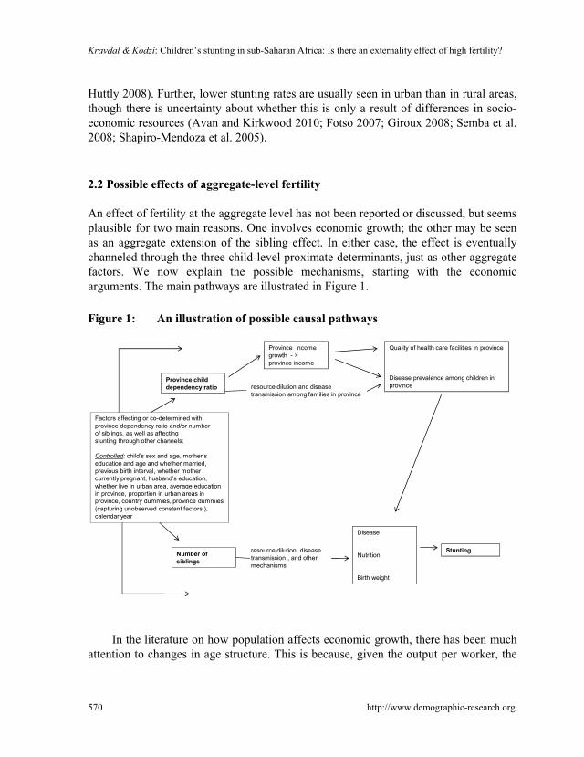
An effect of fertility at the aggregate level has not been reported or discussed, but seems plausible for two main reasons. One involves economic growth; the other may be seen as an aggregate extension of the sibling effect. In either case, the effect is eventually channeled through the three child-level proximate determinants, just as other aggregate factors. We now explain the possible mechanisms, starting with the economic arguments. The main pathways are illustrated in Figure 1.

Figure 1: An illustration of possible causal pathways

Factors affecting or co-determined with province dependency ratio and/or number of siblings, as well as affectingstunting through other channels:

Controlled: child’s sex and age, mother’s education and age and whether married,previous birth interval, whether mothercurrently pregnant, husband’s education, whether live in urban area, average education in province, proportion in urban areas in province, country dummies, province dummies (capturing unobserved constant factors ), calendar year

Province child dependency ratio

Province income growth - > province income

resource dilution and disease transmission among families in province

Number of siblings

Disease

Nutrition

Birth weight

resource dilution, disease transmission , and other mechanisms

Stunting

Quality of health care faciliti

Disease prevalence among province

es in province

children in

In the literature on how population affects economic growth, there has been much

attention to changes in age structure. This is because, given the output per worker, the




output per person is determined by the proportion in the working-age group and proportion who actually work in this age group (e.g. Bloom and Williamson 1998). However, the output per worker may itself depend on various demographic factors, as pointed out already by Coale and Hoover (1958) and later, for example, by Mason (1988). Most importantly, from our perspective, it is possible that an increase in the proportion of young or elderly in the population reduces the output per worker because a larger proportion of the earnings among working-age adults may have to be used to cover childrearing expenses and support for the elderly, resulting in less being saved (as mentioned above). This point has been made by Kelley and Schmidt (2005), who showed that the proportion of young had a negative effect on the growth in the production per worker, given the initial productivity and other factors (while the proportion of elderly had no influence). Generally, higher productivity growth, given the initial level, means a higher current productivity.

In other words, a child who lives in an area where the adults have many children may be at a disadvantage because of a generally low income level. When other people have low income a consequence may be that their children are sick relatively often, and these diseases can be transmitted to the child under study and thus enhance the stunting risk. Further, a higher income in the community may – at least in the somewhat longer run – stimulate, for example, the establishment of health care institutions that any child may benefit from.

The second main mechanism possibly linking high aggregate-level fertility and an individual child’s stunting is an aggregate version of the household-level pathway referred to earlier as the sibling effect, and also bears some resemblance to one of the income related mechanisms just described. The argument runs as follows: when another family has many children, that family may itself experience a high prevalence of diseases (because of the dilution of resources and possible more intense disease transmission within the household), which increases the disease risk for the child under study and ultimately its chance of being stunted.

The number of children a child interacts with outside the household might also affect the chance of being infected. A possible indicator of that could be the number of children within a surrounding area of a certain size, which is determined by the number of households within this area multiplied by the number of children in each household. However, the former probably varies much more than the latter (even given any rural/urban control variable that might be included) and the two are inversely linked to each other, so we hesitate to consider aggregate fertility as affecting an individual child’s chance of being stunted through this mechanism.



3. The basic ideas of the analysis

The goal of the present study is to find out whether there actually is an effect of aggregate fertility, net of number of siblings and other household-level reproductive factors. We should, of course, control as well as possible for factors at different levels that may affect or that are co-determined with aggregate and household fertility in addition to influencing the individual child’s chance of being stunted. For this purpose we use three different approaches, each with their own strengths and weaknesses. These three approaches are further described below. We make no attempt, however, to assess the relative importance of the various pathways that fertility may operate through in affecting individual stunting. Such a task would require data that better reflect the relevant mechanisms, and it is also technically problematic to identify how an individual outcome, such as whether a child has an infectious disease, is affected by the prevalence of that outcome in the community (Kravdal 2003).

It is not easy to conclude from the theoretical arguments what the most appropriate level of aggregation should be. While diseases are transmitted from children nearby, the savings argument may involve the population structure in a small neighbourhood as well as in the country. Dictated by data availability (see explanation below), we have used the province as the level of aggregation. The population size in each province is on average 4 million, varying between 0.2 in Namibia and 26.4 in Nigeria. This level of aggregation may be relevant for the economic-growth mechanism, although less so for the disease-transmission pathway.

Another important but difficult consideration relates to measuring the child dependency burden. According to the mechanisms outlined above, the chance that a child is stunted at the time of an interview depends on nutrition and diseases at any time since its birth, which in turn reflects the general disease pattern and the economic situation at that time. However, the economic situation especially may need some time to be influenced by the burden of childrearing in the population (given the idea that the economic growth during a certain period is influenced by the dependency ratio at the outset through savings), so it would seem reasonable to introduce a long lag in the dependency-ratio variable. We have decided to try two different dependency ratio variables, both of which refer to the province where the child lived when his or her height was measured. One is the average number of children younger than 10 and still alive among the women (aged 15-49) in that province who were interviewed in the survey where the child was measured. The other is the corresponding dependency ratio in the same province according to an earlier survey, typically 5-10 years before. Approach II uses the first of these two dependency ratio variables, while they are used interchangeably in approaches I and III (see further details below). For those who have recently moved from another province, it might be just as reasonable to include the



earlier dependency ratio in that province, but this is not possible with the DHS data. These surveys provide information on how long the family has lived in the primary sampling unit, which typically corresponds to a census enumeration area, but not on whether they have lived in another province earlier. In additional calculations we left out those who had lived in the census enumeration area less than 10 years, and this gave a similar pattern in the estimates.

It is not obvious how the number of siblings should be defined. We have decided to direct our attention largely towards the number of siblings alive and younger than 10 years. Alternative operationalizations gave very similar results (see below for details).

The DHS data include information about some well-established determinants of fertility, such as education and urbanization, which possibly also have a bearing on the stunting risk. In addition to controlling for these and the corresponding province-level averages, we include (in approaches II and III) province dummies to control for additional unobserved province characteristics. When this is not possible (approach I), we include country dummies instead. However, we do not include another potential determinant of fertility, income, because it would have to be proxied by a wealth indicator, which may also to some extent reflect consequences of childbearing (i.e., by doing it we would tap out some of the total effect of fertility that we set out to estimate). This is further explained below, after the data and their limitations have been presented.

4. Data and methods

4.1 Data

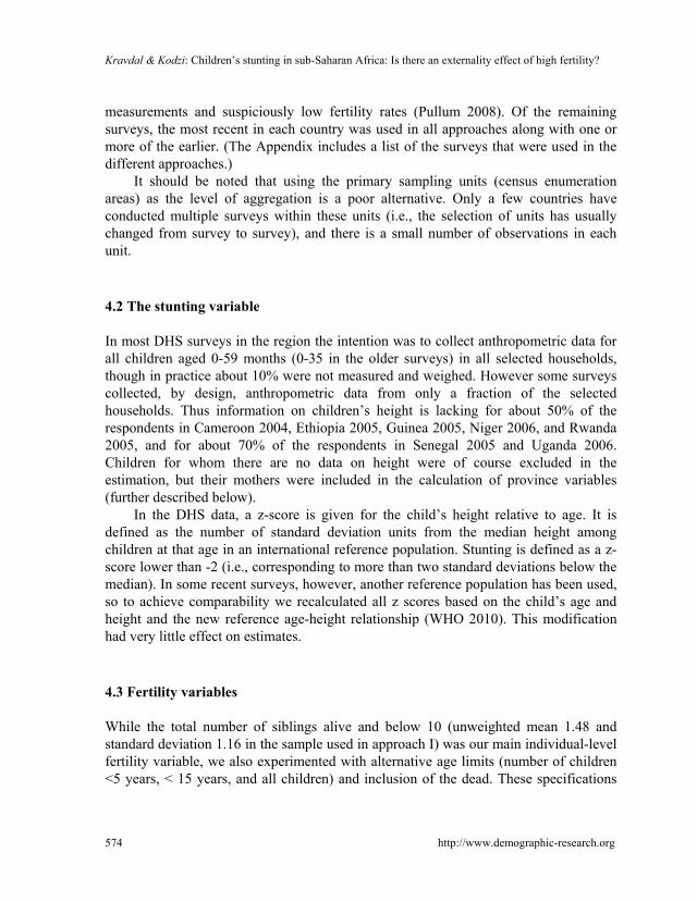
DHS surveys have been conducted in many countries to provide researchers and policy-makers with comprehensive and comparable data on fertility and child health and their determinants. In these surveys women aged 15-49 have been interviewed (and in many countries there has also been a smaller sample of men). We used DHS data (available as of May 2010) from the 23 Sub-Saharan countries that satisfied the following two criteria: first, there had been at least two such surveys with anthropometric measurements in the country; second, the highest-level aggregate units that were defined (typically governorates, provinces, or larger geopolitical zones, but referred to as provinces in this paper) were comparable over at least two surveys.5 In the selected countries, there were 3-12 provinces that were comparable across 2-4 surveys. The Nigerian 1999 survey was excluded because of the poor quality of the anthropometric

5 When the highest level is a geopolitical zone, a larger number of smaller administrative units may have been defined in the data (e.g. for Tanzania, Nigeria, or Kenya), but with relatively few observations in each.



measurements and suspiciously low fertility rates (Pullum 2008). Of the remaining surveys, the most recent in each country was used in all approaches along with one or more of the earlier. (The Appendix includes a list of the surveys that were used in the different approaches.)

It should be noted that using the primary sampling units (census enumeration areas) as the level of aggregation is a poor alternative. Only a few countries have conducted multiple surveys within these units (i.e., the selection of units has usually changed from survey to survey), and there is a small number of observations in each unit.

4.2 The stunting variable

In most DHS surveys in the region the intention was to collect anthropometric data for all children aged 0-59 months (0-35 in the older surveys) in all selected households, though in practice about 10% were not measured and weighed. However some surveys collected, by design, anthropometric data from only a fraction of the selected households. Thus information on children’s height is lacking for about 50% of the respondents in Cameroon 2004, Ethiopia 2005, Guinea 2005, Niger 2006, and Rwanda 2005, and for about 70% of the respondents in Senegal 2005 and Uganda 2006. Children for whom there are no data on height were of course excluded in the estimation, but their mothers were included in the calculation of province variables (further described below).

In the DHS data, a z-score is given for the child’s height relative to age. It is defined as the number of standard deviation units from the median height among children at that age in an international reference population. Stunting is defined as a z-score lower than -2 (i.e., corresponding to more than two standard deviations below the median). In some recent surveys, however, another reference population has been used, so to achieve comparability we recalculated all z scores based on the child’s age and height and the new reference age-height relationship (WHO 2010). This modification had very little effect on estimates.

4.3 Fertility variables

While the total number of siblings alive and below 10 (unweighted mean 1.48 and standard deviation 1.16 in the sample used in approach I) was our main individual-level fertility variable, we also experimented with alternative age limits (number of children <5 years, < 15 years, and all children) and inclusion of the dead. These specifications



gave similar results. Our models also included the interval between the youngest and the second-youngest child, specified categorically, and an indicator of whether the mother was currently pregnant.

Twins were included in the analysis. We observed that they had more than twice as high a chance of being stunted as singletons, but taking that into account by adding a twin control variable or excluding the twins had no impact on other estimates.

As mentioned earlier, the province-level child dependency ratio was calculated either from the survey in which the stunting was measured (and where the individual fertility variables were also taken from) or an earlier survey. In both cases DHS weights (typically constant within units at a lower level than the provinces) were taken into account when aggregating over the individual data. The unweighted mean of the child dependency ratio was 1.54 and the standard deviation 0.30 (approach I). As with the individual-level variable, we experimented with alternative age limits and including the dead, but again, the main conclusions were robust.

Fertility histories in African DHS surveys are mostly complete, and missing information on the timing of births is not a large problem either (Arnold 1990). A potential concern is that many births during the last 5 years before the survey (or 3 in older surveys) have been reported as occurring some months earlier to avoid answering a large number of questions about children. Such displacement of births was particularly common in the surveys from the late 1980s (including the 1988 Togo survey in our analysis; Arnold 1990), and some more recent surveys (Marckwardt and Rutstein 1996). However, potential displacement problems should only affect our interval variable, not the other fertility variables.

4.4 Control variables

4.4.1 Factors that obviously should be controlled for

A number of household-level characteristics may affect the child’s number of siblings, for example through the perceived costs of childbearing, the preferences for alternatives to spending time and money on children, or the access to adequate contraception. If they are also likely to influence the chance of stunting, they should be controlled for. One such factor is the number of completed years of education for the mother, which we included in the models (as a continuous variable). Education may in principle also be influenced by fertility (leading to ‘over-controlling’), but this reverse causation is probably of modest strength in sub-Saharan Africa. We also included the mother’s age (continuous), whether she was married, her partner’s education (continuous), and whether the household lived in a census enumeration area that was characterized as



urban. Further, a detailed control for the child’s age turned out to be quite important, so dummies corresponding to 20 three-month periods were included.6

Also aggregate-level factors may affect individual fertility, in addition to affecting aggregate fertility. Again, women’s education may be an example: it has been shown that a woman’s chance of having a child is influenced by the education of other women in the community (Kravdal 2002). As mentioned earlier, there is also some evidence suggesting an effect of aggregate education on stunting risks. In our models we included the average education and the proportion of urban dwellers among the women in the province who were interviewed (though with some doubt about the latter, as explained below). These variables were calculated from the individual data, as with the child dependency ratio.

The household- and individual-level control variables were taken from the survey in which the child was measured (thus referring to what is called time t below), while the province-level control variables were calculated from the same survey as used for the calculation of the child dependency ratio (which could be the survey at t or an earlier at t’). In additional analysis we included province control variables measured at t’ along with a dependency ratio measured at t, but this gave results very similar to those obtained when all were measured at t.

4.4.2 The wealth indicator

Let us assume now that the interest is in the effect of the child dependency ratio in the province at the time of a previous survey (t’), which reflects fertility during the decade before that. In principle one should include a measure of the income among the (potential) parents in the province some time before that, because it could be a determinant of the dependency ratio and also affect the current stunting risk (at t). The mechanism behind the latter effect is that the income before t’ may affect the growth in the following period (just like the dependency ratio), and hence future income and eventually stunting risks. However, such a lagged income measure is not available in the DHS data. There is information about consumer durables and household amenities at the time of interview (t’), which has often been used to construct a wealth index (Rutstein and Johnson 2004), but such an index would be an indicator of consumption (and hence income) shortly before interview and several years earlier (Bollen, Glanville, and Stecklov 2007; Filmer and Pritchett 2001), and not only the income at the time relevant for fertility (decisions). Including a wealth measure that reflects the

6 Indicators of religion were included in additional models, but were unimportant as controls (though a lower level of stunting was seen among Christians than other religious groups).



income shortly before interview (t’) would be problematic from our perspective because the child dependency ratio at t’ reflects burdens of childrearing before that, which could affect the income shortly before t’ if the suggested effect that involves saving operates quickly enough. In other words, a wealth measure calculated from the survey at t’ can be considered as being, to some extent, on the causal pathway, so we would be ‘over-controlling’. Another reason why we would over-control is that the number of children in other families may affect their ability to purchase consumer goods of importance for the health of the children in that family (an aspect of the ‘resource dilution’ mentioned earlier), with further implications for the children in these families and, ultimately, the stunting risk of a particular child. The average wealth would capture some of this recent consumption among other families and thus be on the causal pathway. There are of course similar arguments against including wealth at the household or province level at time t along with measures of fertility at that time. We therefore did not include any wealth variables in our final model.

Nonetheless, we did some experimentation with a simple wealth index constructed by summing the number of positive answers to the following questions: whether the household members own a radio or a bicycle, whether there is electricity in the house, whether the household has access to piped water or a flush toilet, and whether the floor is made of other materials than dirt.7 In a model where all variables were taken from the most recent survey, we added the province averages of this wealth measure calculated from an earlier survey, which reduces the chance of over-controlling. This alternative model specification gave almost the same effect of the dependency ratio (not shown in the tables).

4.4.3 Unobserved factors

Many unobserved community factors may also influence the level of fertility as well as the individual child’s nutritional status. For example, certain environmental characteristics may have a bearing on food production and also affect the need for child labour. Additional unobserved potential confounders relate to political attitudes (e.g., with respect to health care and family planning programmes) and aspects of the socio-economic development that are poorly captured by the included variables. In approaches II and III we controlled for confounders at the province level that are constant by including province dummies (fixed effects). In approach I we controlled for country-level constant unobserved factors through country dummies.

7 A more advanced pre-constructed wealth measure, based on richer information on consumer durables and household amenities, is available only in the most recent surveys.



The proportion of urban dwellers changes little over time, so one might hesitate to include it in a model with province fixed effects (which requires that other province variables are time-varying), but, fortunately, the key estimates did not depend much on whether this variable was left out.

4.5 Statistical models

Having presented the general ideas of the analysis and the specific variables considered, we now summarize and further specify the three approaches used.

In approach I, we estimated the following logistic regression models for the chance Pijt that child i in province j is stunted at time t, which is the time of the most recent survey (among those it is possible to use):

log (Pijt/(1-Pijt)) = a0 + a1Sijt + a2Fjt’ + a3Xijt + a4Yjt’+ a5Cj + Uj Sijt is a vector of indicators of the mother’s reproductive behaviour up to t (the

child’s number of siblings, length of last birth interval, pregnancy status), and Fjt’ is the child dependency ratio in province j calculated from the oldest survey satisfying our requirements, taking place at time t’ (this is the first-mentioned survey in the list in the Appendix , and conducted on average 10 years before the most recent survey). Xijt is a vector of control variables describing characteristics of the child (age, sex) and its household (whether urban, whether mother married, mother’s and father’s education), and Yjt’ is a vector of province-level control variables at time t’ (average education and average urbanization). Cj are country dummies. The a’s are the corresponding effect coefficients. Uj is a province-level random term (assumed to be drawn independently for each province from a normal distribution with 0 mean and a variance to be estimated) that was added to reflect unobserved constant factors at that level that are unrelated to the other regressors. Including such a random term is standard procedure in multilevel modelling (e.g. Goldstein 2003). It increases standard errors of the effects of province-level variables, but leaves point estimates almost unchanged (there are no differences in linear models and in practice small differences in logistic models). The models were estimated in the MLwiN software.

In another version of approach I we used only data from the most recent survey, i.e., Fjt instead of Fjt’ and Yjt instead of Yjt’.

In approach II, we estimated the model log (Pijt/(1-Pijt)) = b0 + b1Sijt + b2Fjt + b3Xijt + b4Yjt + b5Tt + b6Ej



for children observed in either the most recent or the earliest possible survey (i.e., t refers to the time of one of these surveys). Similar results were found when all surveys were included instead, or when the two most recent ones were included. Ej are province dummies and b6 the corresponding coefficients (province fixed effects). In such a fixed-effects model one cannot include characteristics at the province or higher level that are constant over time, such as the country dummies. Tt is a time variable (equal to t; using one-year dummies gave similar results) that picks up unobserved factors common to all provinces that have changed over time and produced a change in the stunting risk. Leaving the time trend out or interacting it with country dummies did not change the main conclusions. The regressors S, F, X and Y are as in approach I. The models were estimated with the logistic module in the SAS software.

Approach III is a combination of I and II, in the sense that there are both lags and fixed effects. More precisely, we estimated the model

log (Pijt/(1-Pijt)) = c0 + c1Sijt + c2Fjt’ + c3Xijt + c4Yjt’+ c5Tt + c6Ej

for children observed in either the most recent survey or the one before that (i.e., t refers to the time of one of these surveys). t’ refers to the time of the most recent survey before either of these two. In other words, for countries with three surveys this is an analysis of how stunting in the second and third surveys is influenced by the dependency ratio in the first and second survey, respectively. For countries with four surveys we used the second, third, and fourth in a corresponding way. Also these models were estimated in SAS. As with approach I, we estimated an alternative version, with Fjt instead of Fjt’ and Yjt instead of Yjt’.

In all approaches the child under analysis was the youngest living child in the family. There were 82,036 such children included in approach I, 145,116 in approach II, and 60,674 in approach III. In additional analyses we also included the second-last born children alive and measured at interview (without adding a household-level random term, for simplicity). This gave very similar effects.

5. Results

5.1 Effects of fertility variables

Using approach 1, there is a positive but not very large effect of the number of siblings younger than 10: each additional sibling raises the stunting risk (odds) by 2% (Table 1). Further, the expected beneficial effect of a longer birth interval is confirmed. For example, stunting occurs 26% more often among those born less than two years after a



brother or sister than if the interval is three years. There is also an excess chance of stunting if the mother is pregnant.

More importantly, however, there is no significant effect of the child dependency ratio in the province in the earlier survey (but significance was attained when the random term was left out.) In contrast, the effect of the current dependency ratio (included instead of that in the earlier survey) is significant (Table 2). The effects of the number of siblings are the same in these models (Table 2).

Table 1: Effects (odds ratios with 95% CI) of various child, household, and province characteristics on a child’s chance of being stunted, according to approach I

Child’ s age (3-month categories) Not shown Child’s sex (girl=1, boy=0) 0.710*** (0.688-0.733) Number of siblings alive and younger than 10 1.020** (1.003-1.038) Previous birth interval -23 months 1.260*** (1.189-1.334) 24-35 months 1.093*** (1.046-1.143) 36-47 months (ref category) 1 48-59 months 0.929** (0.871-0.992) 60-71 months 0.890*** (0.819-0.969) 72- months 0.877*** (0.809-0.951) Whether mother currently pregnant (yes=1, no=0) 1.058** (1.009-1.140) Mother’s age 0.992*** (0.989-0.995) Mother’s education 0.953*** (0.947-0.958) Whether mother married (yes=1, no=0) 1.048* (0.993-1.107) Her husband’s education (0 if not married) 0.977*** (0.972-0.982) Lives in urban area? (yes=1, no=0) 0.713*** (0.677-0.750) Characteristics of women in the province, measured in earlier survey Average education 0.913*** (0.861-0.968) Proportion urban 1.107 (0.873-1.404) Average number of children alive and younger than 10 1.222 (0.844-1.768) Country dummies Not shown Notes: * p< 0.10; ** p < 0.05; *** p< 0.01. A province-level random term was also included.



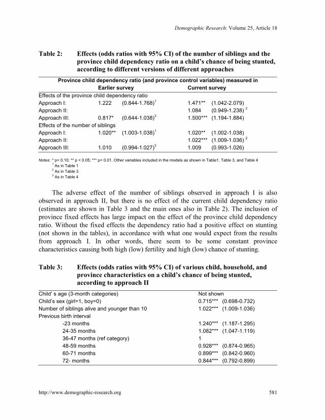
Table 2: Effects (odds ratios with 95% CI) of the number of siblings and the province child dependency ratio on a child’s chance of being stunted, according to different versions of different approaches

Province child dependency ratio (and province control variables) measured in Earlier survey Current survey Effects of the province child dependency ratio Approach I: 1.222 (0.844-1.768)1 1.471** (1.042-2.079) Approach II: 1.084 (0.949-1.238) 2

Approach III: 0.817* (0.644-1.038)3 1.500*** (1.194-1.884) Effects of the number of siblings Approach I: 1.020** (1.003-1.038)1 1.020** (1.002-1.038) Approach II: 1.022*** (1.009-1.036) 2

Approach III: 1.010 (0.994-1.027)3 1.009 (0.993-1.026) Notes: * p< 0.10; ** p < 0.05; *** p< 0.01. Other variables included in the models as shown in Table1, Table 3, and Table 4 1 As in Table 1 2 As in Table 3 3 As in Table 4

The adverse effect of the number of siblings observed in approach I is also

observed in approach II, but there is no effect of the current child dependency ratio (estimates are shown in Table 3 and the main ones also in Table 2). The inclusion of province fixed effects has large impact on the effect of the province child dependency ratio. Without the fixed effects the dependency ratio had a positive effect on stunting (not shown in the tables), in accordance with what one would expect from the results from approach I. In other words, there seem to be some constant province characteristics causing both high (low) fertility and high (low) chance of stunting.

Table 3: Effects (odds ratios with 95% CI) of various child, household, and

province characteristics on a child’s chance of being stunted, according to approach II

Child’ s age (3-month categories) Not shown Child’s sex (girl=1, boy=0) 0.715*** (0.698-0.732) Number of siblings alive and younger than 10 1.022*** (1.009-1.036) Previous birth interval -23 months 1.240*** (1.187-1.295) 24-35 months 1.082*** (1.047-1.119) 36-47 months (ref category) 1 48-59 months 0.928*** (0.874-0.965) 60-71 months 0.899*** (0.842-0.960) 72- months 0.844*** (0.792-0.899)



Table 3: (Continued) Whether mother currently pregnant (yes=1, no=0) 1.023 (0.987-1.061) Mother’s age 0.991*** (0.984-0.993) Mother’s education 0.945*** (0.941-0.949) Whether mother married (yes=1, no=0) 1.038* (0.997-1.081) Her husband’s education (0 if not married) 0.973*** (0.969-0.977) Lives in urban area? (yes=1, no=0) 0.685*** (0.663-0.708) Characteristics of women in the province Average education 0.996 (0.951-1.043) Proportion urban 1.348** (1.033-1.759) Average number of children alive and younger than 10 1.084 (0.949-1.238) Province dummies Not shown Year of interview 0.999 (0.995-1.003) Notes: * p< 0.10; ** p < 0.05; *** p< 0.01

Approach III differs from approach I in four ways: i) only countries with three or

more surveys are included, ii) it is the dependency ratio in the most recent previous surveys that is included rather than that in the earliest survey, iii) the models are estimated not only for the most recent survey but also include the second-most recent, and iv) fixed effects rather than a random effect are included. Yet the results from these two approaches are quite similar in one important respect: there is no significant effect of the lagged child dependency ratio (in fact there are indications of a beneficial effect), while there is an effect of the current child dependency ratio (Tables 2 and 4). However, there is no longer a significant adverse effect of the number of siblings when approach III is used, though the directions of the estimates are maintained.

Table 4: Effects (odds ratios with 95% CI) of various child, household, and

province characteristics on a child’s chance of being stunted, according to approach III

Child’ s age (3-month categories) Not shown Child’s sex (girl=1, boy=0) 0.712*** (0.691-0.733) Number of siblings alive and younger than 10 1.010 (0.994-1.027) Previous birth interval -23 months 1.247*** (1.182-1.316) 24-35 months 1.066*** (1.022-1.112) 36-47 months (ref category) 1 48-59 months 0.915** (0.860-0.973) 60-71 months 0.860*** (0.793-0.932) 72- months 0.870*** (0.805-0.939)



Table 4: (Continued) Whether mother currently pregnant (yes=1, no=0) 1.054** (1.007-1.102) Mother’s age 0.993*** (0.990-0.996) Mother’s education 0.948*** (0.942-0.953) Whether mother married (yes=1, no=0) 1.035 (0.986-1.087) Her husband’s education (0 if not married) 0.969*** (0.964-0.974) Lives in urban area? (yes=1, no=0) 0.687*** (0.660-0.716) Characteristics of women in the province, measured in earlier survey

Average education 1.096*** (1.035-1.162) Proportion urban 0.832 (0.632-1.096) Average number of children alive and younger than 10 0.817* (0.644-1.038) Province dummies Not shown Year of interview 0.985*** (0.977-0.992) Notes: * p< 0.10; ** p < 0.05; *** p< 0.01

As long as we consider the current child dependency ratio and the current level of

the control variables, the only difference between approach III and approach II is that the latter includes more countries and the earliest rather than the second-most recent survey. Nevertheless, the results are quite different, which is somewhat disturbing.

Generally, the effect of the child dependency ratio is little influenced by whether the number of siblings is included, and vice versa (not shown). This reflects that the effects of these two variables are weak and that the correlation between them is not very strong.

5.2 Effects of control variables

The effects of the individual- or household-level control variables are as expected: low odds of stunting are seen for girls, those living in urban census enumeration areas, those having a better-educated mother, and those having older mothers. Consistent with other studies, stunting increases with the child’s age up to about 3 years and then declines (not shown in tables). In combination, the indications of an adverse effect of marriage and the significant beneficial effect of the education of the husband (typically the child’s father) suggests that the child is better off when the mother is single than when she has a husband with a few years of education. The stunting risk is lowest, however, when she has a better educated husband.

The average level of education in the province is inversely related to the stunting risk according to approach I (not only with the specification shown in Table 1, but also



with the two other specifications). In contrast, no effect was observed in approach II, while there were mixed results with approach III (a positive effect when the province variables were lagged and a negative effect when they were not). Therefore one cannot conclude that it helps to live in a community with a generally high level of education. It is possible that the advantages of being surrounded by better-educated individuals with a low disease prevalence and good knowledge of nutrition and child care may be outweighed by disadvantages stemming from a low relative position in society.

There are no other significant province-level effects, except that living in a highly urbanized province increases the risk of stunting according to approach II. This contrasts with the beneficial effect of living in an urban census enumeration area and might suggest a resource competition with an urban bias, in the sense that, for example, the health care in a rural area is less developed when it is competing with many urban areas in the province. Alternatively, there may be problems with the inclusion of a province-level urbanization variable because of its modest variation over time (see earlier comment).

6. Summary and conclusion

It does not seem unreasonable to expect that high fertility in a province, or at another level of aggregation, may influence a child’s chance of stunting adversely, above and beyond any effect of own family size (reported in earlier studies and confirmed in some of our models). As explained in more detail above, such an aggregate-level effect may reflect, for example, a lower savings rate in a population where there are many dependants. This may lead to lower income growth and thus a lower general income later. A lower income among other families may increase the chance that the children in these families are sick and thus the risk that the child under investigation gets sick and eventually becomes stunted, and the general income level may also affect the quality of the health care services in the area. Such adverse economic effects of high fertility have been assumed by many politicians and researchers, though without overwhelming empirical support. Furthermore, high fertility among other families may more directly increase the disease prevalence in these families, with implications for an individual child’s stunting risk.

In our analysis of 23 countries in sub-Saharan Africa we see no effects of the child dependency ratio in the province at the time of an earlier survey, typically 5-10 years before. There is more support for an adverse effect of the current dependency ratio. This may suggest that the economic mechanism, which probably needs more time to play out, is of little importance, while the effect of other community members’ high fertility operating through a more direct enhancement of the disease load among their children



may matter more. That said, there may be unobserved determinants of the province fertility that also affect the individual child’s stunting risk. The fixed effects modelling certainly helps to reduce such problems, but only picks up the constant province-level unobserved factors. There may also be time-varying unobserved province characteristics that affect both fertility and stunting. One such potentially confounding factor is the income level in the province. We included a wealth variable in an additional model (lagging it, while all other variables referred to the current situation, to reduce the chance of over-controlling). This had very little impact on the estimates of the fertility effects, but the wealth variable is admittedly a rather crude indicator of the economic resources. In principle, fertility and stunting may be influenced in different directions or in the same direction by the unobserved factors. In the latter case, the true effect of fertility will be even less adverse than indicated by the estimates. Moreover, there is a disturbing lack of robustness in our estimates, in the sense that the selection of countries and surveys seems to matter. All in all, one should therefore be hesitant to state that there is an effect of the overall fertility level on an individual child’s nutritional status.

To conclude, we think we have raised an important question. Stunting is obviously a key welfare indicator that deserves continued attention, and it can be quite easily measured (as opposed to, for example, income or purchasing power). The idea that other community members’ fertility may be among its determinants has not been checked so far, but seems plausible. In fact such a mechanism would be part of a broader externality effect of high fertility that has often been taken for granted, and that has motivated population policies in several countries, but which has still not been backed up by very strong statistical evidence. We have used data of supposedly high quality, and have stretched the analysis as much as possible by using three alternative approaches that allow us to consider lagged effects, control for constant unobserved province-level factors, or (with a smaller sample) do both. However, there is no clear empirical conclusion. A fair summary of the estimates would be that there are only weak indications of an adverse effect of the general fertility level. This blurred empirical picture indicates that researchers should continue to address the question with better tools before policy conclusions are drawn. In particular, it would be an advantage to have data that include better control variables and encompass a larger number of aggregate units at the province level, and that also permit consideration of lower levels of aggregation that might be more relevant for some of the causal effects potentially involved.



7. Acknowledgements

Comments from two anonymous reviewers and the associate editor, Andrew Hinde, are greatly appreciated. The analysis has been funded by the Hewlett Foundation and the Norwegian Research Council (grant number 199475).



References

Aaby, P. (1988). Malnutrition and overcrowding / Intensive exposure in severe measles infection: Review of community studies. Reviews of Infectious Diseases 10(2): 478-491. doi:10.1093/clinids/10.2.478.

Adair, L.S. and Guilkey, D. (1997). Age-specific determinants of stunting in Filipino children. The Journal of Nutrition 127(2): 314-320.

Alderman, H., Hentschel, J., and Sabates, R. (2003). With the help of one’s neighbors: Externalities in the production of nutrition in Peru. Social Science and Medicine 56(10): 2019-2031. doi:10.1016/S0277-9536(02)00183-1.

Anh, T.S., Knodel, J., Lam, D., and Friedman, J. (1998). Family size and children’s education in Vietnam. Demography 35(1): 57-70. doi:10.2307/3004027.

Arnold, F. (1990). Assessment of the quality of birth history data in the Demographic and Health Surveys. In Assessment of DHS-I Data Quality, Institute of Resource Development (IRD). Columbia, Maryland: IRD, DHS Methodological Reports (Number 1).

Avan, B.I. and Kirkwood, B. (2010). Role of neighbourhoods in child growth and development. Social Science and Medicine 71: 102-109.

Black, R., Morris, S., and Bryce, J. (2003). Where and why are 10 million children dying every year? The Lancet 361(9376): 2226-2234. doi:10.1016/S0140-6736(03)13779-8.

Bloom, D. and Williamson, J. (1998). Demographic transitions and economic miracles in emerging Asia. World Bank Economic Review 12(3): 419-456. doi:10.1093/ wber/12.3.419.

Boerma, J.T. and Bicego, G.T. (1992). Preceding birth intervals and child survival: searching for pathways of influence. Studies in Family Planning 23(4): 243-256.

Bollen, K.A., Glanville, J.L., and Stecklov, G. (2007). Socioeconomic status, permanent income, and fertility: A latent-variable approach. Population Studies 61(1): 15-34. doi:10.1080/00324720601103866.

Bronte-Tinkew, J. and DeJong, G.F. (2004). Children’s nutrition in Jamaica: Do household structure and household economic resources matter? Social Science and Medicine 58(3): 499-514. doi:10.1016/j.socscimed.2003.09.017.

Burström, B., Diderichsen, F., and Smedman, L. (1999). Child mortality in Stockholm during 1885-1910: The impact of household size and number of children in the

http://dx.doi.org/10.1093/clinids/10.2.478

http://dx.doi.org/10.1016/S0277-9536(02)00183-1

http://dx.doi.org/10.2307/3004027

http://dx.doi.org/10.1016/S0140-6736(03)13779-8

http://dx.doi.org/10.1016/S0140-6736(03)13779-8

http://dx.doi.org/10.1093/wber/12.3.419

http://dx.doi.org/10.1093/wber/12.3.419

http://dx.doi.org/10.1080/00324720601103866

http://dx.doi.org/10.1016/j.socscimed.2003.09.017



family on the risk of death from measles. American Journal of Epidemiology 149: 1134-1141.

Cardoso, M.R.A., Cousens, S.N., Siqueira, L.F.G., Alves, F.M., and D’Angelo, L.A.V. (2004). Crowding: Risk factor or protective factor for lower respiratory disease in young children. BMC Public Health 2004(4): 19. doi:10.1186/1471-2458-4-19.

Chang, S.M., Walker, S., Grantham-McGregor, S., and Powell, C. (2002). Early childhood stunting and later behaviour and school achievement. Journal of Child Psychology and Psychiatry 43(6): 755-783.

Cleland, J., Bernstein, S., Ezeh, A., Faundes, A., Glasier, A., and Innis, J. (2006). Family planning: the unfinished agenda. The Lancet 368(9549): 1810-1827. doi:10.1016/S0140-6736(06)69480-4.

Coale, A.J. and Hoover, E. (1958). Population Growth and Economic Development in Low-Income Countries. Princeton, NJ: Princeton University Press.

Eloundou-Enyegue, P. and Williams, L. (2006). The effects of family size on child schooling in sub-Saharan settings: A reassessment. Demography 43(1): 25-52. doi:10.1353/dem.2006.0002.

Filmer, D. and Pritchett, L.H. (2001). Estimating wealth effects without expenditure data - or tears: an application to educational enrolments in states of India. Demography 38(1): 115-132. doi:10.1353/dem.2001.0003.

Fortney, J. and Higgins, J. (1984). The effect of birth interval on perinatal survival and birth weight. Public Health 98(2): 73-83. doi:10.1016/S0033-3506(84)80099-2.

Fotso, J.C. (2007). Urban-rural differentials in child malnutrition: Trends and socioeconomic correlates in sub-Saharan Africa. Health & Place 13(1): 205-223. doi:10.1016/j.healthplace.2006.01.004.

Fotso, J.C. and Kuate-Defo, B. (2005). Socioeconomic inequalities in early childhood malnutrition and morbidity: modification of the household-level effects by the community SES. Health & Place 11(3): 205-225. doi:10.1016/j.healthplace. 2004.06.004.

Frost, M.B., Forste, R., and Haas, D.W. (2005). Maternal education and child nutritional status in Bolivia: Finding the links. Social Science and Medicine 60(2): 395-407. doi:10.1016/j.socscimed.2004.05.010.

Giroux, S. (2008). Child stunting across schooling and fertility transitions: Evidence from sub-Saharan Africa. DHS Working Papers (2008-57).

http://dx.doi.org/10.1186/1471-2458-4-19

http://dx.doi.org/10.1186/1471-2458-4-19

http://dx.doi.org/10.1016/S0140-6736(06)69480-4

http://dx.doi.org/10.1353/dem.2006.0002


http://dx.doi.org/10.1016/S0033-3506(84)80099-2

http://dx.doi.org/10.1016/j.healthplace.2006.01.004






Glewwe, P., Jacoby, H., and King, E. (2001). Early childhood nutrition and academic achievement: A longitudinal analysis. Journal of Public Economics 81(3): 345-368. doi:10.1016/S0047-2727(00)00118-3.

Goldstein, H. (2003). Multilevel Statistical Models. London: Arnold.

Graff, M., Yount, K.M., Ramakrishnan, U., Martorell, R., and Stein, A.D. (2010). Childhood nutrition and later fertility: Pathways through education and pre-pregnant nutritional status. Demography 47(1): 125-144. doi:10.1353/ dem.0.0090.

Grantham-McGregor, S., Cheung, Y.B., Cueto, S., Glewwe, P., Richter, L., and Strupp, B. (2007). Developmental potential in the first 5 years for children in developing countries. The Lancet 369(9555): 60-70. doi:10.1016/S0140-6736(07)60032-4.

Headey, D.K. and Hodge, A. (2009). The effect of population growth on economic growth: A meta-regression analysis of the macroeconomic literature. Population and Development Review 35(2): 221-248. doi:10.1111/j.1728-4457.2009. 00274.x.

Hernandez-Diaz, S., Peterson, K.E., Dixit, S., Hernandez, B., Parra, S., Barquera, S., Sepulveda, J., and Rivera, J.A. (1999). Association of maternal short stature with stunting in Mexican children: common genes vs. common environment. European Journal of Clinical Nutrition 53(12): 938-945.

Kelley, A.C. and Schmidt, R.M. (1995). Aggregate population and economic growth correlations: The role of the components of demographic change. Demography 32(4): 543-555.

Kelley, A.C. and Schmidt, R.M. (2005). Evolution of recent economic-demographic modelling: A synthesis. Journal of Population Economics 18(2): 275-300. doi:10.1007/s00148-005-0222-9.

Kinugasa, T., Huang, W., and Yamaguchi, M. (2007). Demographic change and regional economic growth: A comparative analysis of Japan and China. In: Mason, A. and Yamaguchi, M. (eds.). Population Change, Labor Markets and Sustainable Growth: Towards a New Economic Paradigm. Elsevier.

Kravdal, Ø. (2002). Education and fertility in sub-Saharan Africa: Individual and community effects. Demography 39(2): 233-250. doi:10.1353/dem.2002.0017.

Kravdal, Ø. (2003). The problematic estimation of “imitation effects” in multilevel models. Demographic Research 9(2): 25-40. doi:10.4054/DemRes.2003.9.2.

http://dx.doi.org/10.1016/S0047-2727(00)00118-3



http://dx.doi.org/10.1016/S0140-6736(07)60032-4

http://dx.doi.org/10.1111/j.1728-4457.2009.00274.x

http://dx.doi.org/10.1111/j.1728-4457.2009.00274.x

http://dx.doi.org/10.1007/s00148-005-0222-9


http://dx.doi.org/10.4054/DemRes.2003.9.2



Larrea, C. and Kawachi, I. (2005). Does income inequality affect child malnutrition? The case of Equador. Social Science and Medicine 60(1): 165-178. doi:10.1016/j.socscimed.2004.04.024.

Li, H. and Zhang, J. (2007). Do birth rates hamper economic growth? The Review of Economics and Statistics 89(1): 110-117. doi:10.1162/rest.89.1.110.

Li, H., Zhang, J., and Zhu, Y. (2008). The quantity-quality trade-off of children in a developing country: Identification using Chinese twins. Demography 45(1): 223-243. doi:10.1353/dem.2008.0006.

Mapa, D.S., Balisacan, A.M., and Briones, K.J.S. (2006). Robust determinants of income growth in the Philippines. Philippine Journal of Development 33(1-2).

Marckwardt, A.M. and Rutstein, S.O. (1996). Accuracy of DHS-II demographic data: Gains and losses in comparison with earlier surveys. DHS Working Papers (Number 19).

Mason, A. (1988). Savings, economic growth and population change. Population and Development Review 14(1): 113-144.

Mendez, M.A. and Adair, L.S. (1999). Severity and timing of stunting in the first two years of life affect performance on cognitive tests in late childhood. The Journal of Nutrition 129(8): 1555-1562.

Moestue, H. and Huttly, S. (2008). Adult education and child nutrition: the role of family and community. Journal of Epidemiology and Community Health 2008(62): 153-159. doi:10.1136/jech.2006.058578.

Montgomery, M. and Lloyd, C. (1996). Fertility and child health. In: Ahlburg, D., Kelley, A.C., and Mason, K. (eds.). The impact of population growth on well-being in developing countries. Berlin: Springer.

Pullum, T.W. (2008). An assessment of the quality of data on health and nutrition in the DHS surveys, 1993-2003. Calverton, Maryland, USA: Macro International Inc., Methodological Reports (number 6).

Rahman, A. and Chowdhury, S. (2007). Determinants of chronic malnutrition among preschool children in Bangladesh. Journal of Biosocial Science 39(171-173). doi:10.1017/S0021932006001295.

Ricci, J.A. and Becker, S. (1996). Risk factors for wasting and stunting among children in Metro Cebu, Philippines. American Journal of Clinical Nutrition 63(6): 966-975.


http://dx.doi.org/10.1162/rest.89.1.110


http://dx.doi.org/10.1136/jech.2006.058578

http://dx.doi.org/10.1017/S0021932006001295



Rutstein, S.O. and Johnson, K. (2004). The DHS wealth index. Calverton, Maryland, USA: ORC Macro, DHS Comparative Reports (Number 6).

Semba, R.D., de Pee, S., Sun, K., Sari, M., Akhter, N., and Bloem, M.W. (2008). Effect of parental formal education on risk of child stunting in Indonesia and Bangladesh: a cross-sectional study. The Lancet 371(9609): 322-328. doi:10.1016/S0140-6736(08)60169-5.

Shapiro-Mendoza, C., Selwyn, B.J., Smith, D.P., and Sanderson, M. (2005). Parental pregnancy intention and early childhood stunting: findings from Bolivia. International Journal of Epidemiology 34(2): 387-396. doi:10.1093/ije/dyh354.

Shroff, M., Griffiths, P., Adair, L., Suchindran, C., and Bentley, M. (2009). Maternal autonomy is inversely related to child stunting in Andhra Pradesh, India. Maternal and Child Nutrition 5(1): 64-74. doi:10.1111/j.1740-8709.2008. 00161.x.

Sommerfelt, A.E. and Stewart, M.K. (1994). Children’s nutritional status. Calverton MD: Macro International, DHS Comparative Studies (Number 12).

Ukwuani, F. and Suchindran, C. (2003). Implications of women’s work for child nutritional status in sub-Saharan Africa: A case study of Nigeria. Social Science and Medicine 56: 2109-2121.

UNICEF (2010). Nutrition statistics. http://www.unicef.org/rightsite/sowc/pdfs/ statistics/SOWC_Spec_Ed_CRC_TABLE%202.%20NUTRITION_EN_111309.pdf.

Wamani, H., Åstrøm, A.H., Peterson, S., Tumwine, J.K., and Tylleskär, T. (2007). Boys are more stunted than girls in sub-Saharan Africa: A meta analysis of 16 demographic and health surveys. BMC Pediatrics 7(17). doi:10.1186/1471-2431 -7-17.

Weinreb, L., Wehler, C., Perloff, J., Scott, R., Hosmer, L., Sagor, L., and Gundersen, C. (2002). Hunger: Its impact on children’s health and mental development. Pediatrics 110(4 Oct): 41-50. doi:10.1542/peds.110.4.e41.

WHO (2010). The WHO Child Growth Standards. www.who.int/childgrowth/ standards.

Zhu, B.P. (2005). Effects of interpregnancy interval on birth outcomes. Findings from three recent US studies. International Journal of Gynecology and Obstetrics 89(S1): S25-S33. doi:10.1016/j.ijgo.2004.08.002.

http://dx.doi.org/10.1016/S0140-6736(08)60169-5

http://dx.doi.org/10.1093/ije/dyh354

http://dx.doi.org/10.1111/j.1740-8709.2008.00161.x

http://dx.doi.org/10.1111/j.1740-8709.2008.00161.x

http://www.unicef.org/rightsite/sowc/pdfs/�statistics/SOWC_Spec_Ed_CRC_TABLE 2. NUTRITION_EN_111309.pdf



http://dx.doi.org/10.1186/1471-2431-7-17

http://dx.doi.org/10.1186/1471-2431-7-17

http://dx.doi.org/10.1542/peds.110.4.e41

http://www.who.int/childgrowth/�standards

http://www.who.int/childgrowth/�standards

http://dx.doi.org/10.1016/j.ijgo.2004.08.002



Zhu, B.P., Haines, K.M., Le, T., McGrath-Miller, K., and Boulton, M.L. (2001). Effect of the interval between pregnancies on perinatal outcomes among white and black women. American Journal of Obstetrics and Gynecology 185(6): 1403-1410. doi:10.1067/mob.2001.118307.

http://dx.doi.org/10.1067/mob.2001.118307



Appendix

A list of countries and provinces included in the analysis is shown below. The surveys (indicated by the year of the survey) that are used in approaches I and II are underlined, while those that are used in approach III are in italics. DHS surveys that have become available after May 2010 have not been used. BENIN: 1996, 2001, 2006

Atacora, Atlantique, Borgou, Mono, Oueme, Zou

BURKINA FASO: 1993, 1999 Ouagadougou, North, East, West, Central/South

CAMEROON: 1991, 1998, 2004 Yaounde/Douala, Adam/Nord/Ext-Nord, Centre/Sud/Est, Ouest/Littoral, Nord-Ouest/Sud-Ouest

CHAD: 1997, 2004 Zone 1 – Zone 8

ETHIOPIA: 2000, 2005 Tigray, Affar, Amhara, Oromiya, Somali, Ben-Gumz, SNNP, Gambela, Harari, Addis, Dire Dawa

GHANA: 1993, 1998, 2003, 2008 Western, Central, Greater Accra, Volta, Eastern, Ashanti, Brong-Ahafo, Northern, Upper West, Upper East

GUINEA: 1999, 2005 Lower Guinea, Central Guinea, Upper Guinea (High), Forest Guinea, Conakry

KENYA: 1993, 1998, 2003 (2003: without the North Eastern region, which was not included in earlier surveys, and Eastern and Rift Valley regions slightly redefined to accord with earlier surveys) Nairobi, Central, Coast, Eastern, Nyanza, Rift Valley, Western

MADAGASCAR: 1992, 1997, 2004 Antananarivo, Fianarantsoa, Toamasina, Mahajanga, Toliary, Antsiranana

MALAWI: 1992, 2000, 2004 Northern, Central, Southern



MALI: 1996, 2001, 2006 (2001 and 2006: without the Kedal region, which had not been included earlier) Kayes, Koulikoro, Sikasso, Segou, Mopti, Timbuktu, Gao, Bamako

MOZAMBIQUE: 1997, 2003 Niassa, Cabo Delgado, Nampula, Zambezia, Tete, Manica, Sofala, Inhambane, Gaza, Maputo, Cidade de Maputo

NAMIBIA: 2000, 2007 Caprivi, Erongo, Hardap, Karas, Khomas, Kunene, Ohangwena, Kavango, Omaheke, Omusati, Oshana, Oshikoto, Otjozondjupa

NIGER: 1992, 1998, 2006 Niamey, Dosso, Maradi, Tahoua/Agadez, Tillaberi, Zinda/Diffa

NIGERIA: 2003, 2008 North Central, North East, North West, South East, South West, South South

RWANDA: 1992, 2000, 2005 Kigali, Northwest, Southwest, Central/South, Northeast

SENEGAL: 1993, 2005 West, Central, South, North East

TANZANIA: 1996, 1999, 2005 Coastal, Northern Highlands, Lake, Central, Southern Highlands, South, Zanzibar

TOGO: 1988, 1998 Maritime (inc Lome), Des Plateaux, Centrale, De la Kara, Des Savanes

UGANDA: 1995, 2001, 2006 Central, Eastern, Northern, Western

ZAMBIA: 1992, 1996, 2002, 2007 Central, Copperbelt, Eastern, Luapula, Lusaka, Northern, North-Western, Southern, Western

ZIMBABWE: 1994, 1999, 2006 Manicaland, Mashonaland Central, Mashonaland East, Mashonaland West, Watabeleland North, Matabeleland South, Midlands, Masvingo, Harare/Chitungwiza, Bulawayo

children's stunting in sub-saharan africa: is there an ... · table of contents 1 introduction...

Documents