christopher conrad 1,*, sebastian fritsch 1 · was carried out on pan-sharpened spot data. varying...

Remote Sens. 2010, 2, 1035-1056; doi:10.3390/rs2041035

Remote Sensing ISSN 2072-4292

www.mdpi.com/journal/remotesensing Article

Per-Field Irrigated Crop Classification in Arid Central Asia Using SPOT and ASTER Data

Christopher Conrad 1,*, Sebastian Fritsch 1 , Julian Zeidler 1 , Gerd Rücker 2 and Stefan Dech 1,2

1 Remote Sensing Unit, University of Wuerzburg, Am Hubland, 97074 Wuerzburg, Germany;

E-Mails: [email protected] (S.F.); [email protected] (J.Z.) 2 German Aerospace Center (DLR), German Remote Sensing Data Center (DFD), Oberpfaffenhofen,

82234 Wessling, Germany; E-Mails: [email protected] (G.R.); [email protected] (S.D.)

* Author to whom correspondence should be addressed; E-Mail: [email protected];

Tel.: +94-931-31-81875; Fax: +94-931-888-4960.

Received: 17 February 2010; in revised form: 22 March 2010 / Accepted: 23 March 2010 /

Published: 8 April 2010

Abstract: The overarching goal of this research was to explore accurate methods of

mapping irrigated crops, where digital cadastre information is unavailable: (a) Boundary

separation by object-oriented image segmentation using very high spatial resolution

(2.5–5 m) data was followed by (b) identification of crops and crop rotations by means of

phenology, tasselled cap, and rule-based classification using high resolution (15–30 m)

bi-temporal data. The extensive irrigated cotton production system of the Khorezm

province in Uzbekistan, Central Asia, was selected as a study region. Image segmentation

was carried out on pan-sharpened SPOT data. Varying combinations of segmentation

parameters (shape, compactness, and color) were tested for optimized boundary separation.

The resulting geometry was validated against polygons digitized from the data and

cadastre maps, analysing similarity (size, shape) and congruence. The parameters shape

and compactness were decisive for segmentation accuracy. Differences between crop

phenologies were analyzed at field level using bi-temporal ASTER data. A rule set based

on the tasselled cap indices greenness and brightness allowed for classifying crop rotations

of cotton, winter-wheat and rice, resulting in an overall accuracy of 80 %. The proposed

field-based crop classification method can be an important tool for use in water demand

estimations, crop yield simulations, or economic models in agricultural systems similar to

Khorezm.

OPEN ACCESS

Remote Sens. 2010, 2

1036

Keywords: object-based classification, segmentation, tasselled cap, Uzbekistan, irrigated

agriculture, multi-sensor

1. Introduction

Sustainable land and water management is essential for securing food production under the situation

of climate change, decreasing water resources and growing population especially in the face of limited

arable land [1]. Accurate crop distribution maps can substantially support this effort as they contribute

to three important aspects: planning, modelling, and monitoring of land and water allocation in

agriculture. For these applications, remote sensing has proven to be a valuable tool in the past decades.

Especially for mapping crop distributions and rotations, numerous image classification algorithms

have been developed [2]. However, optimization of classification accuracies is an ongoing process and

advances in sensor technology, new image processing techniques as well as increasing computing

capacities allow for perpetual improvements of existing classification concepts and methods.

The use of mono-temporal, multi-spectral data has proven to be largely unsuitable for agricultural

land use classification due to the spectral similarity of crops at certain cropping stages. Multi-temporal

methods are better suited for crop mapping because they consider the phenological development of

crops [3,4]. Due to their high temporal resolution, medium spatial resolution sensors like AVHRR [5]

and MODIS [6,7] have been widely used. However they are only applicable at regional scales or for

large homogeneous fields [8]. High spatial resolution sensors like Landsat-TM/ETM+ or

SPOT-5-HRG provide less recurrence, but allow for a more detailed discrimination of agricultural land

use at field scale [9], especially in regions where small-scale farming prevails.

For such regions, object-oriented techniques were found superior to pixel-based classifications [10,11].

Small-scale differences in crop growth (e.g., due to uneven irrigation or saline patches) may easily

lead to misclassifications at pixel level. The concept of field-based crop classifications accounts for the

observed heterogeneity in the spectral signals of agricultural fields [12], which may be caused by

spatially varying plant water, nutrient or pest infection stress, soil colors, or vegetation density. Field

boundaries are used to homogenise intra-field patterns. Per-field classifiers [13] combine vector and

raster information to GIS-ready information [14].

In existing studies on per-field classification, vector information on field boundaries was derived

from ancillary layers mostly digitized from satellite images, cadastral data, or topographic

maps [11,12]. However, if large areas are to be mapped and ancillary data is unavailable, segmentation

techniques can be used to derive agricultural fields from raster data for subsequent classification [14].

The authors in [15] e.g., utilized high resolution aerial images to derive landscape objects in northern

Italy, whereas the within-object classification was based on satellite imagery. But altogether, studies

applying such multi-sensor approaches per-field classification methods are still rare.

The quality of image segmentation is decisive for every ensuing object-based image classification [16].

The challenge is to find the optimal segmentation parameters, as to derive image objects which

resemble real world objects as closely as possible. In most remote sensing studies, segmentations have

been evaluated, in order to avoid over- or under-segmentation, either visually [15] or by using complex


1037

(mathematical) approaches [17,18]. With regard to the subsequent classification simple and practicable

quality estimation metrics are highly desirable.

Independent of the origin of the field boundaries, the crop type for the field-object is mostly

assigned by integrating the results of an underlying pixel-based land use classification. [12] and [11]

first classified the crop type of each pixel. Calculating the modal class or majority of the underlying

pixels led to the classification decision at field level. In [15] a more complex rule set based on several

features for object classification, such as the predominant class, area of the predominant class, number

of pixels within an object, etc. was developed. In contrast, [14] classified field-averaged

spectral reflectances.

1.1. Objectives

This study focuses on accurate per-field classifications of crops in irrigation systems, where digital

cadastre information is unavailable or lacking in quality. It was conducted on irrigated croplands in the

Khorezm region, Uzbekistan. In this region, accurate information on crop distribution and crop

rotation are essential for estimations of water demand and the prediction of crop yields.

The first objective was to derive agricultural field boundaries from high resolution satellite data

(SPOT 5, 2.5–5 m) by utilizing image segmentation techniques. The use of high resolution data for

segmentation has also been considered advantageous by [15], because medium resolution data

(15–30 m) often result in less accurate segmentation results. Special emphasis was on an objective

procedure for selecting appropriate segmentation settings (optimization of field geometry). By

achieving this target, all other non-agricultural land use or land cover classes such as settlements,

desert, or water bodies can be omitted from subsequent classifications.

We secondly aimed at the classification of crop types and crop rotations within the field boundaries

using multi-temporal data of medium spatial resolution (bi-temporal ASTER, 15–30 m) and analysing

tasselled cap indices in a rule-based approach. The idea was to analyse the composition of vegetation

cover and soil wetness within a field and its temporal development during different phenological

stages (cropping calendar). According to [19] the tasselled cap indices brightness and greenness were

assumed to represent soil wetness and green vegetation cover (vegetation density), respectively.

In theory it is desirable to have multiple images over the growing season for crop classification.

Bi-temporal data was selected to account for two cropping seasons and to minimize data costs, because

relatively cheap high resolution solutions can more easily be adopted by land and water managers in

Central Asia. We want to show that by carefully selected acquisition dates two data sets suffice for

accurately mapping winter and summer crops occurring in the Uzbek study area.

2. Study Area

The Khorezm province is located in the Aral Sea Basin between the Amu Darya River to the north

and the Turkmen border to the south (see Figure 1a). The climate is dry and continental and the region

belongs to the zones of deserts and steppes [20]. On average, approximately 100 mm of annual

precipitation falls, predominantly during winter with high spatial and temporal variability. Annual

potential evapotranspiration is approximately 1,500 mm [21].


1038

Figure 1. The study area. (a) Countries and irrigation regions of Central Asia. The

Khorezm region is highlighted. (b) Administrative boundaries of the Rayons in the

Khorezm region and the extent of the satellite images used in this study. (c) Boundaries of

the Water User Associations (WUAs) in Khorezm. The SPOT 5 scenes used in this study

are displayed in the background. Highlighted are the WUAs that are investigated in this

study (1: Jayhun; 2: Amir Temur; 3: Shomahulum; 4: P. Mahmud; 5: Madir Yop).

Khorezm represents a major cotton production system of the former Soviet Union which is facing

serious economic and ecological problems [22]. Since the independency of Uzbekistan 1991, demand

on the scarce water resources has been increasing due to the introduction of winter-wheat for

self-sufficiency. Soil quality in the region is low, shallow and saline groundwater in combination with

inappropriate management practices, formerly described by [23], further increase the soil salinity [24]

throughout the region. Furthermore, Khorezm is strongly affected by periodic droughts and resulting

shortages in irrigation water supply. Altogether, sustainable land and water management is hardly

achievable, since crop production is strongly dependent on an adequate supply of fertilizers and water.

The region comprises an area of roughly 5,600 km2, approximately 2,750 km2 are used for irrigated

agriculture [25]. Dominant crop types are cotton, winter wheat and rice, constituting around 70–80%

of the arable lands. A schematic cropping calendar for these crops is presented in Figure 2. Wherever

possible, another crop is grown on the winter-wheat fields after harvest, mostly rice. Fodder maize,

alfalfa, sunflower as well as fruits and vegetables are also cultivated, but their allotment is

comparatively low [26].


1039

Khorezm is subdivided into eleven administrative units, so-called Rayons (Figure 1b). The

irrigation system is managed and maintained by so-called Water User Associations (WUAs,

Figure 1c), which comprise numerous private farms. The classification was carried out on a subset

from the Amu Darya River in the north-east to the desert in the south-west. It was defined by the

intersection between the Khorezm region and the extent of the ASTER and SPOT 5 data (Figure 1b).

Five WUAs located in this area were selected for sampling (Figure 1c). It will be shown in Section

3.3.1., that this transect encompasses large parts of the ecological variability of all WUAs in Khorezm.

Field boundaries however, were delineated for the entire extend of the SPOT scenes (see Figure 1b).

Figure 2. Idealized cropping calendar of the study region, Khorezm.

3. Materials and Methods

The conceptual framework of this study comprises two major parts, illustrated in Figure 3. At first,

field boundaries were derived from mono-temporal high resolution SPOT 5 data by segmentation. The

segmentation was optimized using the geometry of digitized reference fields and cadastre maps.

Secondly, the resulting polygons were subsequently classified into fields and other objects and

validated against the same vector information. The classification decision for each field-parcel was

based on bi-temporal ASTER data. The tasseled cap indices greenness and brightness served as

features for classifying basic cover types indicating the vegetation density and soil wetness of each

pixel (sparse, medium, and dense vegetation; dry and wet soil). Bi-temporal information of vegetation

density and soil wetness was then analyzed within the field-parcels using ground-truth samples and the

cropping calendar (Figure 2) to establish a rule-base for the final classification. It has to be noted, that

in regions, where digital field boundaries are available, the extraction of the field-parcels using high

resolution remote sensing data can be omitted.


1040

Figure 3. Schematic workflow of the study. The left part shows the separation of field

boundaries for per-field classification, the right part highlights the classification steps.

Note: the segmentation of field boundaries can be replaced by any other source of vector

field boundaries.

Separation of field boundaries

Pan‐mergedSPOT (2.5‐5m)

Digitizedcadastre

Segmentation

Field‐identification

Crop classification

Bi‐temporalASTER (15‐30m)

Fieldsamples

Tasseled Cap

Basic cover types(pixel based)

Rule baseValid

ation

Opt.

Fieldparcels

Rulegen

eration

Valid

ation

Crop distribution map

Separation of field boundaries

Pan‐mergedSPOT (2.5‐5m)

Digitizedcadastre

Segmentation

Field‐identification

Crop classification

Bi‐temporalASTER (15‐30m)

Fieldsamples

Tasseled Cap

Basic cover types(pixel based)

Rule baseValid

ation

Opt.

Fieldparcels

Rulegen

eration

Valid

ation

Crop distribution map

The following sections contain a description of the satellite data and the preprocessing, and both

methodological parts, the separation of the field boundaries and the crop classification.

3.1. Satellite Data and Pre-Processing

Field boundaries were derived from SPOT 5 High Resolution Geometric (HRG) data. In Khorezm

most field boundaries coincide with irrigation or drainage canals. Thus, they were considered constant

for a couple of years which is in agreement with the assumption of [12]. SPOT images were acquired

mid-season in 2006 (Table 1), after wheat harvest and before cotton reached full vegetation cover.

Wheat and cotton fields were therefore dry and bare. The remaining fields were either flooded for rice

cultivation or covered by secondary crops (Figure 2). ASTER images, used for crop classification,

were recorded twice during the growing season 2007, nearly time-synchronous to ground truthing.

Two dates of imagary were selected in order to distinguish between winter and summer crops, in

particular different crop rotations of wheat.


1041

Table 1. Characteristics of the ASTER and SPOT images used in this study.

Sensor

Characteristics

SPOT 5-HRG

[27]

Terra-ASTER

[28]

Product level 1B—Radiance at sensor 1B—Radiance at sensor

Number of scenes 2 4

Date of image collection 19. / 22.06.2006 01.06.2007 (2)

03.07.2007 (2)

Bands used* PAN (1), VNIR (3), SWIR (1) VNIR (3), SWIR (6)

Spatial resolution [m] 2.5, 10, 20 15, 30

Swath width [km] 60–80 60

* PAN = PANchromatic band; VNIR = Visible and Near InfraRed spectra, SWIR = Short Wave

InfraRed spectra

The first pre-processing steps consisted of atmospheric and geometric corrections. Despite

relatively good atmospheric conditions, the ASTER imagery was atmospherically corrected to be able

to apply one rule set to both images [29]. ATCOR 6.4 [30] was used for correction. The aerosol type

was set to ‘dry rural’ and the calibration coefficients for ASTER were selected according to [31].

SPOT PANchromatic (PAN) images were corrected for atmospheric influences to sharpen the contrast

between the mostly dry fields and the vegetated canals at the field boundaries. SPOT PAN scenes were

subsequently ortho-rectified using the software XDibias [32] and eight ground control points per

image based on differential GPS measurements. The rectification resulted in sub-pixel accuracies of

the images. Afterwards SPOT Multi-Spectral (MS) and ASTER scenes were fitted to the PAN images

using a second order polynomial model and 24 to 32 ground control points per image, collected

on-screen. Final geo-location accuracy was also below one pixel. In support of the segmentation

described below, a 5 × 5 variance texture image was calculated from SPOT PAN data. Moreover, a

pan-sharpening of the SPOT data was conducted using a High Pass Filter (HPF) algorithm [33].

3.2. Segmentation of Agricultural Fields Using Pan-Sharpened SPOT Data

A layerstack of pan-sharpened SPOT data and the variance texture image was segmented and

subsequently classified into fields and non-fields using the software Definiens Developer 7. Two

parameters control the segmentation process in Definiens: the scale parameter (controlling object size)

and the relation between object compactness and smoothness [16]. To determine optimal parameter

settings for segmentation, several combinations of parameters were tested and validated against actual

field boundaries (see also [17]).

The range of possible values for the scale parameter was set by visual inspection of different

segmentation results. The multi-resolution segmentation algorithm was applied [34] with the following

scale parameters: 70, 90, 110 and 130. These were combined with three color (0.9, 0.7, and 0.5) and

three shape (0.5, 0.7, and 0.9) parameters. Altogether, 36 (4 × 3 × 3) different segmentation settings

were tested.

Five representative WUAs (see Section 3.3.1.) and 10 randomly selected square subsets with a size

of 2.5 × 2.5 km each served for validation. Reference field boundaries were manually digitized from

the pan-sharpened SPOT data and cross-checked with official land register maps, if available.


1042

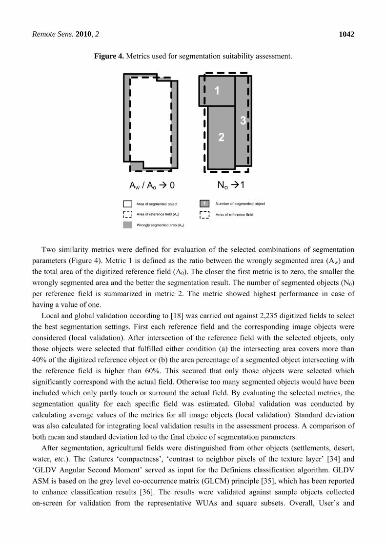
Figure 4. Metrics used for segmentation suitability assessment.

Two similarity metrics were defined for evaluation of the selected combinations of segmentation

parameters (Figure 4). Metric 1 is defined as the ratio between the wrongly segmented area (Aw) and

the total area of the digitized reference field (A0). The closer the first metric is to zero, the smaller the

wrongly segmented area and the better the segmentation result. The number of segmented objects (N0)

per reference field is summarized in metric 2. The metric showed highest performance in case of

having a value of one.

Local and global validation according to [18] was carried out against 2,235 digitized fields to select

the best segmentation settings. First each reference field and the corresponding image objects were

considered (local validation). After intersection of the reference field with the selected objects, only

those objects were selected that fulfilled either condition (a) the intersecting area covers more than

40% of the digitized reference object or (b) the area percentage of a segmented object intersecting with

the reference field is higher than 60%. This secured that only those objects were selected which

significantly correspond with the actual field. Otherwise too many segmented objects would have been

included which only partly touch or surround the actual field. By evaluating the selected metrics, the

segmentation quality for each specific field was estimated. Global validation was conducted by

calculating average values of the metrics for all image objects (local validation). Standard deviation

was also calculated for integrating local validation results in the assessment process. A comparison of

both mean and standard deviation led to the final choice of segmentation parameters.

After segmentation, agricultural fields were distinguished from other objects (settlements, desert,

water, etc.). The features ‘compactness’, ‘contrast to neighbor pixels of the texture layer’ [34] and

‘GLDV Angular Second Moment’ served as input for the Definiens classification algorithm. GLDV

ASM is based on the grey level co-occurrence matrix (GLCM) principle [35], which has been reported

to enhance classification results [36]. The results were validated against sample objects collected

on-screen for validation from the representative WUAs and square subsets. Overall, User’s and


1043

Producer’s accuracy were calculated according to [37]. All subsequent work was based on the

resulting agricultural field layer.

3.3. Per-Field Irrigated Crop Classification

3.3.1. Ground Truth Data

Ground truthing was carried out from May to July 2007. In order to balance the need for sufficient

data with costs, WUAs representing the environmental variability in terms of climate, irrigation water,

and ecological settings were chosen as appropriate sampling locations. The environmental situation

was assumed to encompass differences in crop growth patterns. Therefore, a statistical stratification of

the WUAs in the Khorezm region was applied. Average data on soil quality, soil salinity, groundwater

level (indicating the location properties), distance from water intake points (potential water supply),

evapotranspiration (actual water consumption) and rice-cropped area (permanent water availability)

served as input. The data was provided by the central database of the ZEF/UNESCO Khorezm

project [38].

For stratification a hierarchical cluster analysis followed by a K-means cluster analysis was

conducted on all 119 WUAs. Five clusters were chosen to be representative of the study region. For

ground truth data collection, one WUA was selected for each cluster (Figure 1c). Within each WUA, a

cluster sampling scheme [39] was applied to receive an acceptable number of reference datasets for

classification. This sampling method fulfils the requirements of a probability sampling design, thus

allowing for subsequent statistical analysis and an appropriate accuracy assessment [40]. In total, 253

fields were sampled comprising the following crop types: ‘Cotton’ (99), ‘Wheat’ (78), ‘Rice’ (74),

‘Wheat-rice’ (47), ‘Fallow’ (41) and ‘Other’ (29).

3.3.2. Per-Pixel Derivation of Vegetation Density and Soil Wetness

At the start of a cropping period, agricultural fields are usually bare, which is followed by an

increase of green vegetation cover and turns to yellow upon the ripening state of crops. The tasselled

cap (TC) indices brightness, greenness, yellowness reflect this course of varying environmental state

within a remote sensing pixel over agricultural areas [41]. According to the concept of [19], the TC

index brightness represents the soil line, which allows for the separation of dry and wet soil in regions

where colors of dry soil are homogeneous. Analogous the greenness can be understood as a “green

stuff vector” showing the cover of green vegetation within one pixel [19]. We used this concept to

simply categorize the density of green vegetation within one pixel and—in case of no vegetation

cover—the soil wetness. The area portions of the resulting five basic land cover classes within one

field were later used for the final crop classification (Section 3.3.3.).


1044

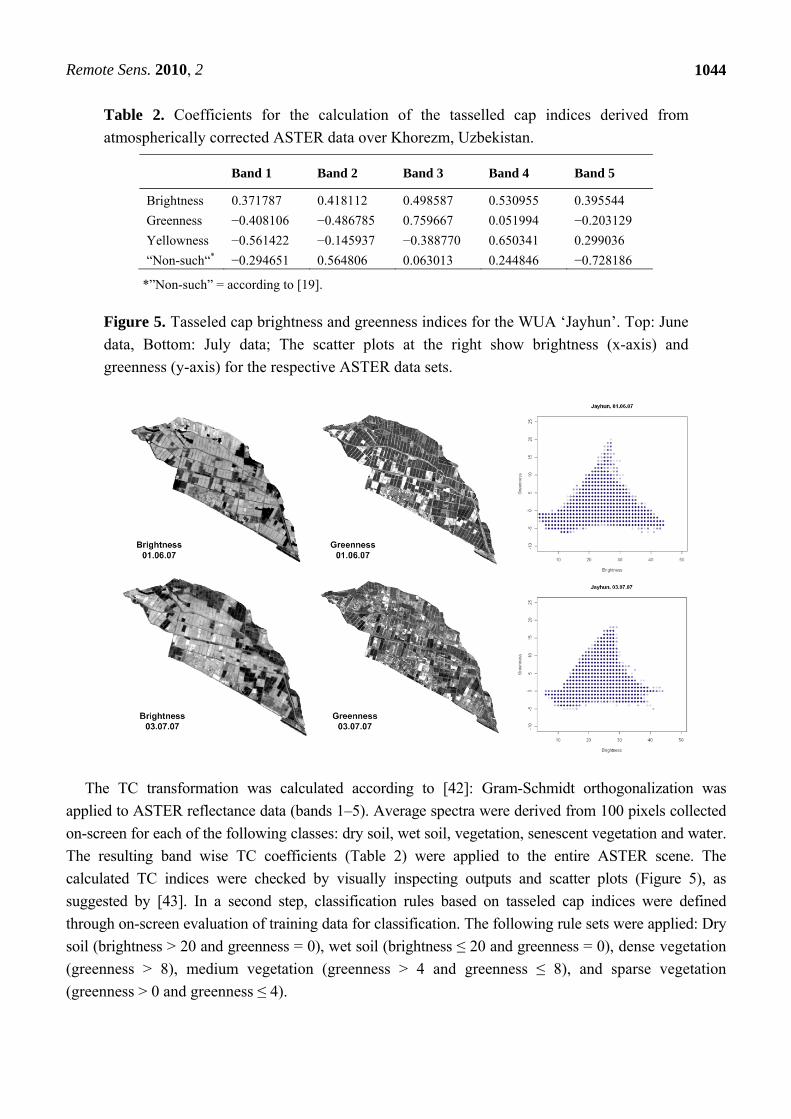
Table 2. Coefficients for the calculation of the tasselled cap indices derived from

atmospherically corrected ASTER data over Khorezm, Uzbekistan.

Band 1 Band 2 Band 3 Band 4 Band 5

Brightness 0.371787 0.418112 0.498587 0.530955 0.395544

Greenness −0.408106 −0.486785 0.759667 0.051994 −0.203129

Yellowness −0.561422 −0.145937 −0.388770 0.650341 0.299036

“Non-such“* −0.294651 0.564806 0.063013 0.244846 −0.728186

*”Non-such” = according to [19].

Figure 5. Tasseled cap brightness and greenness indices for the WUA ‘Jayhun’. Top: June

data, Bottom: July data; The scatter plots at the right show brightness (x-axis) and

greenness (y-axis) for the respective ASTER data sets.

The TC transformation was calculated according to [42]: Gram-Schmidt orthogonalization was

applied to ASTER reflectance data (bands 1–5). Average spectra were derived from 100 pixels collected

on-screen for each of the following classes: dry soil, wet soil, vegetation, senescent vegetation and water.

The resulting band wise TC coefficients (Table 2) were applied to the entire ASTER scene. The

calculated TC indices were checked by visually inspecting outputs and scatter plots (Figure 5), as

suggested by [43]. In a second step, classification rules based on tasseled cap indices were defined

through on-screen evaluation of training data for classification. The following rule sets were applied: Dry

soil (brightness > 20 and greenness = 0), wet soil (brightness ≤ 20 and greenness = 0), dense vegetation

(greenness > 8), medium vegetation (greenness > 4 and greenness ≤ 8), and sparse vegetation

(greenness > 0 and greenness ≤ 4).


1045

3.3.3. Per-Field Crop Classification

Based on the bi-temporal basic land cover classification, a classification of crop rotations was

conducted on the field-object level. Rules were derived using ground truth data and expert knowledge

(cropping calendar, Figure 2). The ground truth data was divided into two halves. One half supported

visual interpretation and rule generation, the other accuracy assessment. The rule set was also

implemented with Definiens Developer 7. The feature ‘relative area of sub-objects’ [34] was used to

analyze land cover changes (phenology) between the image acquisition dates. For each field, area

percentages of all five basic cover classes were derived by summarizing the underlying pixel-levels.

Analysis of tables and bar plots (Figure 6) showing relative area of dry soil, wet soil, and dense,

medium, and sparse vegetation within the training fields allowed the development of general rules

(Figure 7). De Wit et al. [11] similarly derived a decision tree but from multi-temporal NDVI data

averaged per field. The classification was done in a sequential way.

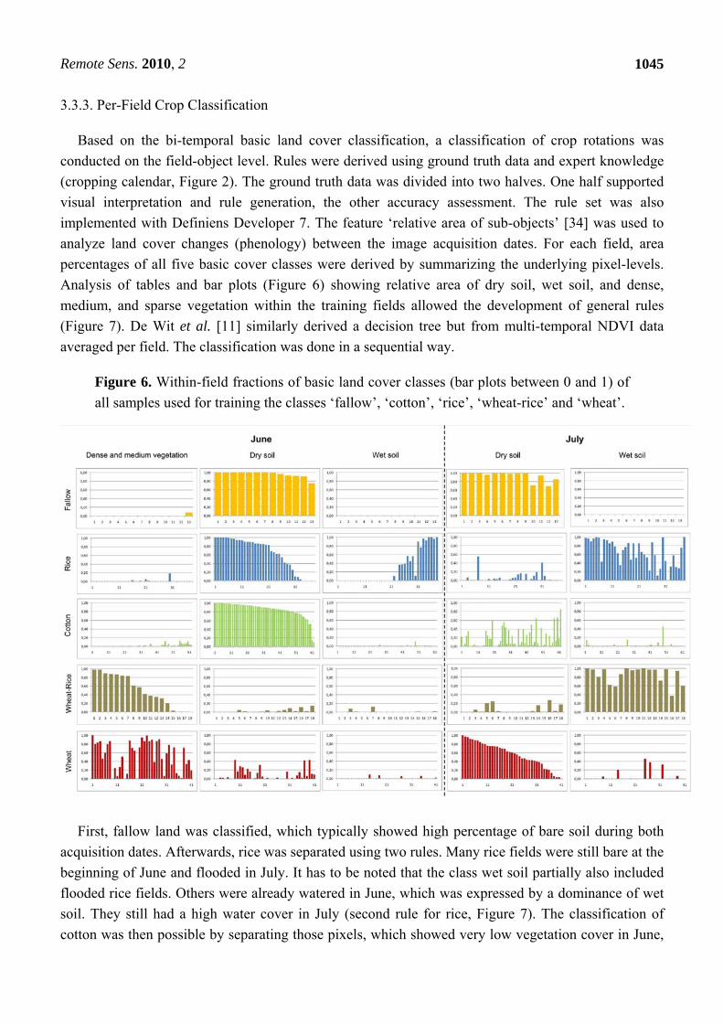
Figure 6. Within-field fractions of basic land cover classes (bar plots between 0 and 1) of

all samples used for training the classes ‘fallow’, ‘cotton’, ‘rice’, ‘wheat-rice’ and ‘wheat’.

First, fallow land was classified, which typically showed high percentage of bare soil during both

acquisition dates. Afterwards, rice was separated using two rules. Many rice fields were still bare at the

beginning of June and flooded in July. It has to be noted that the class wet soil partially also included

flooded rice fields. Others were already watered in June, which was expressed by a dominance of wet

soil. They still had a high water cover in July (second rule for rice, Figure 7). The classification of

cotton was then possible by separating those pixels, which showed very low vegetation cover in June,


1046

mainly expressed by high area percentages of dry soil. High vegetation cover in June was primarily

used to classify winter-wheat in rotation with rice. Other rotations of wheat were identified by

separating pixels with high percentage of bare soil in July. The remaining pixels were classified to the

class ‘other’. The further extraction of clear rules failed, because they only showed confusing patterns.

Some benchmarks were adjusted after the validation, if too many pixels expected to be in the class

‘other’ were misclassified.

Figure 7. Rule base for final classification at field level. Note: DS = dry soil, WS = wet

soil, D&MV = dense and medium vegetation, t1 = first ASTER record (01.06.2007),

t2 = second ASTER record (03.07.2007)

It has to be noted that the cropping calendar was only partly useful for rule generation. It is an

average scheme with high inter-annual variations due to varying water availability in the study area.

Especially for cotton, the year 2007 deviated strongly from that scheme. Climate data showed a

delayed start of season, because the frost period was elongated and daily minimum temperatures did

not exceed 10 °C until the end of May. Temperatures above 10° C are essential for cotton cultivation

in Khorezm [44]. In average years, those cultivations can be expected in the beginning of May. Thus,

the rules had to be adjusted to actual environmental conditions.


1047

4. Results and Discussion

The first part of the result chapter comprises the segmentation results. Focus is set on the evaluation

of the segmentation parameters and the separation of agricultural fields from non-fields. Afterwards,

the rule-based per-field classification is presented, analyzed, and discussed. The accuracy assessments

are reflected against the background of environmental variability in the Khorezm region.

4.1. Segmentation and Generation of the Field Layer

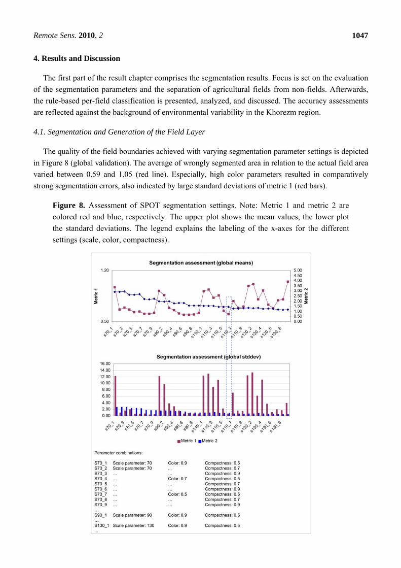
The quality of the field boundaries achieved with varying segmentation parameter settings is depicted

in Figure 8 (global validation). The average of wrongly segmented area in relation to the actual field area

varied between 0.59 and 1.05 (red line). Especially, high color parameters resulted in comparatively

strong segmentation errors, also indicated by large standard deviations of metric 1 (red bars).

Figure 8. Assessment of SPOT segmentation settings. Note: Metric 1 and metric 2 are

colored red and blue, respectively. The upper plot shows the mean values, the lower plot

the standard deviations. The legend explains the labeling of the x-axes for the different

settings (scale, color, compactness).


1048

An increased scale parameter intensified this effect. This pattern emphasizes that segmentation

accuracy in agricultural areas is mostly dependent on the shape of the fields.

On the other hand, comparatively small shape parameters led to significant over-segmentation, as

shown by metric 2 (blue line). There was a consequent decrease from 2.94 to 1.17 objects generated

per field, induced by increasing shape parameters and decreasing influence of multispectral

information (colors) during the segmentation process. The optimum value of one was nearly reached

for the largest scale parameters applied (130). However, comparatively high values of metric 1 clearly

indicate errors in location and size of the segmented objects, if only one object was derived for each

field. The impact of standard deviations of metric 2 (blue bars) was found negligible for selecting

optimum segmentation settings.

The setting S110_60 is a compromise between a small average number of segments representing a

single field and acceptable segmentation errors. The selected parameter combination corresponds with

the following Definiens settings: scale parameter 110, color 0.7 and compactness 0.9. The total area

error of all segments in relation to the digitized field boundaries averaged at 0.6. This error seems to be

high, but it can be explained by the 1.44 polygons which were segmented for each digitized field

(metric 2). Additional visual assessments proved the chosen settings to be closest to reality but also

disclosed major problems of the segmentation.

In Khorezm fields are usually surrounded by irrigation and drainage channels with vegetated slopes.

Because of the sharp contrast, bare fields were persistently segmented more accurately than fields

covered by vegetation or water. Segmentation errors mostly stem from boundaries between fields not

being wide enough to be significant at SPOT resolution. In case of currently flooded and vegetated

neighboring fields one segment often comprised two or more actual fields. On the other hand one

actual field could be covered by more than one segmented objects. Partly flooded or vegetated fields

featured additionally a much stronger spatial variability in their spectra, which bolstered

over-segmentation and thus further reduced accuracy.

Table 3. Accuracy assessment for the separation of agricultural fields using SPOT data.

Subset name Prod.’s accuracy User’s accuracy Overall accuracy Validation

object class

‘field’

Validation

object class ‘no

field’

East 1 0.98 0.98 0.98 57 50

East 2 0.90 0.87 0.89 53 59

East 3 0.96 0.90 0.93 50 57

East 4 0.91 0.96 0.92 69 44

East 5 0.91 0.76 0.83 60 77

West 1 0.96 0.97 0.96 75 62

West 2 0.89 0.92 0.90 68 63

West 3 0.79 0.84 0.84 68 87

West 4 0.94 0.95 0.94 94 70

West 5 0.94 0.85 0.86 67 41

Amir Temur 0.93 0.99 0.95 191 116


1049

Table 3. Cont.

Jayhun 0.98 0.89 0.92 185 149

Madir Yop 0.93 0.95 0.94 133 111

P. Mahmud 0.92 0.85 0.89 138 154

Shomahulum 0.82 0.95 0.85 318 155

Total 0.92 0.91 0.91 1909 1448

Given the wide range of approaches for the validation of segmentation, it is generally difficult to

directly compare results of different studies. In [45] a similar measure to compare the field geometries

after segmentation with digitized field boundaries was utilized and an accuracy of 87% was achieved.

For comparison we implemented the same technique and resulted in 81 % for the finally selected

segmentation settings (S110_60). However, the results remain hardly comparable, because [45]

integrated existing official cadastre information into a three-step segmentation optimization routine

applied to Landsat TM data in large-scale agriculture of the Netherlands. The approach presented in

this study targeted to regions where such information is unavailable.

The negative effect of vegetation and soil wetness observed during the geometry assessments

became even more evident when distinguishing between fields and non-fields. The accuracy of this

initial classification was assessed by sampling 3357 reference objects on-screen. The overall

accuracy [37] for all validation objects was 0.91 (Table 3) and varied slightly between the selected

WUAs and the ten validation squares (see Section 3.2). Again, problems mainly occurred with fields

covered by vegetation or water. For instance, subset East 5 characterized by flooded and partly also

abandoned fields showed a relatively low accuracy of 0.83 for field/non-field separation, whereas East

1 dominated by bare fields achieved 0.98.

The consequences of reduced spectral contrast were also reflected in the comparison of WUA

statistics (from digitized fields) and the segmented objects (Table 4). The number of fields digitized

was generally lower than the number of objects categorized as agricultural fields. WUAs with a high

proportion of vegetated or flooded fields at image acquisition time, such as the WUAs Madir Yop or P.

Mahmud, exhibit a disproportional number of segmented fields.

Table 4. Object-based statistics of the investigated WUAs resulting from SPOT

segmentation and field identification.

WUA Characteristic

Jayhun

Amir

Temur

Shoma-

hulum P. Mahmud

Madir

Yop

Size of WUA (ha) 3,927 3,004 4,042 2,503 2,618

No. of fields in WUA (digitized) 699 435 589 418 186

Situation

SPOT

No. of bare fields 363 243 248 226 80

No. of vegetated/flooded

fields 336 192 341 192 106

Results No. of generated objects 2,270 1,688 2,241 2,105 1,156

No. of classified fields 760 535 733 594 356

Altogether segmentation quality and subsequent field classification are strongly dependent on the

land cover of the agricultural fields at the overpass date. Using more than one satellite image for the


1050

generation of the field layer would be one solution to further reduce errors in both, segmentation and

field-masking. An additional image should consequently be acquired for a period when fields which

are vegetated or flooded on the first image are bare. A manual correction of segmentation errors may

also be a viable solution for smaller extents.

In total, 142,201 objects with an average size of 2.59 ha and a standard deviation of 11.22 ha were

generated for the study area (see Figure 1). The classification based on bi-temporal ASTER data was

finally conducted for 84,311 agricultural fields (average area: 1.88 ha) extracted from all objects

(Section 3.3).

4.2. Per-Field Crop Classification

The analysis of basic land cover information acquired from ASTER data at two time steps during

the vegetation period resulted in per-field crop distribution maps of the study area, exemplified in

Figure 9. The final map (Figure 10) shows the spatial distribution of crop types in the study area.

Figure 9. Per-field crop map of the WUA Jayhun (close to the Amu Darya River) derived

from bi-temporal ASTER data.

The overall accuracy of the classification was 80 % (Table 5). The identification of crop rotations

with winter-wheat, rice and cotton and the localization of fallow land performed mostly above average.

Lowest accuracies were found for the class other. This is partially due to the fact that this class is very

heterogeneous encompassing multiple crops with different spatial & spectral characteristics and

phenology. An adequate number of training samples and one or two additional acquisition dates would

be essential for a better discrimination of this class and a better integration into the classification rules.

The confusion matrix additionally indicates that the knowledge-based classification scheme probably

needs additional options to classify single classes or some automation to avoid overfitting to the

training samples. A relatively high portion of cotton and rice samples missed all rules and ended up in

the class “other”.


1051

Figure 10. Map showing the per-field crop distribution over the entire study area derived

from bi-temporal ASTER data recorded in 2007.

Table 5. Accuracy assessment of the crop distribution maps at object level: confusion

matrix, user’s & producer’s accuracy and overall accuracy.

Cotton Rice Wheat Wheat-

Rice Fallow Other Sum

User’s

accuracy

Cotton 31 0 0 0 3 4 38 0.816

Rice 0 30 1 0 0 0 31 0.968

Wheat 0 0 30 3 0 9 42 0.714

Wheat-Rice 0 5 0 26 0 0 31 0.839

Fallow 0 0 0 0 24 0 24 1.000

Other 6 5 2 0 1 16 30 0.533

Sum 37 40 33 29 28 29 196

Prod.’s accuracy 0.838 0.750 0.909 0.897 0.857 0.552 Overall:

0.801


1052

The same problem with a collective class for crops covering minor area portions (‘other crops’) was

observed by [11]. Final accuracy of this classification carried out in the Netherlands based on Landsat

scale was around 90 %, and seven agricultural classes were distinguished. The reasons for the slightly

higher accuracy of those investigations are most likely threefold. In [11] image segmentation was

deemed too inaccurate but had the advantage of existing digital cadastre maps. They observed the

phenological cycle on a higher level of detail, because a third image acquisition date was available

during the cropping season. The within-field heterogeneity of crop growth can be assumed reduced in

rainfed agriculture areas like the Netherlands. In Khorezm, however, a patchwork of growing

conditions could be observed within single fields, which were caused by non-uniform supply of

irrigation water and fertilizers or spatial variability of soil salinity.

In [12] in contrast, crop rotations was classified at field level in Turkey, where fields were partly

under irrigation. They received overall accuracy of 81 % which is similar to the presented findings.

Three Landsat acquisition dates were classified to distinguish eleven crop types. It can be assumed that

the thematic level of detail could have been increased in the presented study if more image

acquisitions were available. However, the agrodiversity in Khorezm is pretty low compared to other

agricultural regions. For the task of mapping the dominating rotations of cotton, rice, and wheat, two

ASTER satellite images proved to be sufficient. In summary, it seems inappropriate to directly

compare different per-field classification methodologies, since tasks, requirements, agro-ecosystems

etc. usually differ widely.

The impact of the ecological and infrastructural settings represented by the cluster analysis (see

Section 3.3.1.) on the classification results was negligible. Only producer’s accuracy for the class

wheat-rice was below average for the WUAs P. Mahmud and Shomahulum. Both WUAs are located in

downstream positions of the irrigation network and sometimes expect retarded water supply [46].

Delayed wheat harvest likely shifted field preparation (flooding) for rice beyond the second ASTER

image acquisition. Therefore the classification rules might not have been optimal in this case, however,

the number of samples within the single WUAs were generally too low for substantial interpretation.

Unsurprisingly, cotton (50,000 ha) was evenly distributed throughout the entire region. This reflects

the overall importance of cotton as the dominant export commodity. Rice fields (25,000 ha) on the

other hand, were mainly located along the Amu Darya and in the south, where numerous small lakes

and river-like collectors are located. Wheat-rice rotations (10,000 ha) and other crops (30,000 ha)

appeared disproportionately in the East of the study area, in the surroundings of the capital Urgench

and the city Khonka. Another reason for this intensive use (fields include for example rotations of

wheat with maize or sunflowers and wheat intercropping with mulberry trees) is the high reliability of

water supply in central Khorezm [46]. Wheat followed by fallow or crop rotations with minor

vegetation coverage were also mapped nearly evenly throughout the region (26,000 ha). Fallow lands

(13,700 ha) were concentrated to the west of Urgench and close to the desert in the South, where fields

are marginal and soils sandy.

The spatial cropping patterns strongly coincide with previous findings in the same study region

by [6]. Their classification, based on MODIS NDVI time series of the year 2004, exhibited the same

spatial distribution of cotton, rice fields and winter-wheat crop rotations.


1053

5. Conclusions

In this study, a multi-sensor concept was designed to support classifications of mainly wheat, rice,

and cotton rotations in the irrigation system of Khorezm, Uzbekistan. The concept consisted of two

steps: (a) the delineation of field boundaries using very high resolution satellite data and (b) the

classification of multi-temporal medium resolution satellite data for distinguishing crops and crop

rotations within each field object. The first part was designed for regions where digital cadastre

information are unavailable. The approach was implemented using 2.5 m SPOT, and bi-temporal

15–30 m ASTER data.

An objective selection of segmentation settings was proposed to accurately delineate agricultural

fields. The suggested metrics for comparisons of the segmented geometry (similarity-size, shape- and

congruence) indicated a high potential for an objective assessment and selection of the optimum

segmentation settings. Despite optimization of segmentation settings, geometric discrepancies were

persistent due to environmental conditions blurring field boundaries. Multi-temporal segmentation

approaches are still an outstanding research but they might minimize such effects and could also

improve to distinguish between fields and non-field objects (e.g., settlements, deserts, water bodies).

An overall accuracy of 80 % confirmed the success of the selected per-field classification rule-base

applied to analysis of within-field land cover composition (vegetation cover, soil wetness) categorized

for both ASTER acquisitions. In theory, the usage of the tasseled cap indices greenness (representing

the density of green vegetation cover) and brightness (soil wetness) makes the developed rule-set very

flexible and transferable, because it can be applied independently of a specific sensor system. With a

few adaptations, such as the integration of additional image acquisitions, the introduction of automated

classification methods, or the use of new sensor constellations covering more area than ASTER, the

approach of the Khorezm region can be easily transferred to other irrigation systems of Central Asia

and beyond.

Acknowledgements

This study was partly funded by the German Academic Exchange Service (DAAD) and carried out

within the framework of the German-Uzbek ZEF/UNESCO project on ‘economical and ecological

restructuring of land and water use in the Khorezm region, Uzbekistan’, funded by the German

Ministry for Education and Science (BMBF) under project number 0339970C.

References and Notes

1. Biradar, C.M.; Thenkabail, P.S.; Platonov, A.; Xiao, X.M.; Geerken, R.; Noojipady, P.; Turral,

H.; Vithanage, J. Water productivity mapping methods using remote sensing. J. Appl. Remote

Sens. 2008, 2, 1-22.

2. Martinez-Casasnovas, J.A.; Martin-Montero, A.; Casterad, M.A. Mapping multi-year cropping

patterns in small irrigation districts from time-series analysis of Landsat TM images. Eur. J.

Agron. 2005, 23, 159-169.

3. Fuller, D.O. Trends in NDVI time series and their relation to rangeland and crop production in

Senegal, 1987–1993. Int. J. Remote Sens. 1998, 19, 2013-2018.


1054

4. Ramankutty, N.G.; Graumlich, L.; Achard, F.; Alves, D.; Chhabra, A.; DeFries, R.S.; Foley, J.A.;

Geist, H.; Houghton, R.A.; Goldewijk, K.K.; Lambin, E.F.; Millington, A.; Rasmussen, K.; Reid,

R.S.; Turner, B.L., II. Global land-cover change: recent progress, remaining challenges. In Land-Use

and Land-Cover Change-Local Processes and Global Impacts; Lambin, E.F., Geist, H.J., Eds.;

Springer: Berlin, Germany, 2006; p. 222.

5. Jakubauskas, M.E.; Legates, D.R.; Kastens, J.H. Crop identification using harmonic analysis of

time-series AVHRR NDVI data. Comput. Electron. Agric. 2002, 37, 127-139.

6. Conrad, C.; Dech, S.W.; Hafeez, M.; Lamers, J.; Martius, C.; Strunz, G. Mapping and assessing

water use in a Central Asian irrigation system by utilizing MODIS remote sensing products. Irrig.

Drainage Syst. 2007, 21, 197-218.

7. Wardlow, B.D.; Egbert, S.L.; Kastens, J.H. Analysis of time-series MODIS 250 m vegetation

index data for crop classification in the US Central Great Plains. Remote Sens. Environ. 2007,

108, 290-310.

8. Fritz, S.; Massart, M.; Savin, I.; Gallego, J.; Rembold, F. The use of MODIS data to derive

acreage estimations for larger fields: A case study in the south-western Rostov region of Russia.

Int. J. Appl. Earth Obs. Geoinf. 2008, 10, 453-466.

9. Guerschman, J.P.; Paruelo, J.M.; Di Bella, C.; Giallorenzi, M.C.; Pacin, F. Land cover

classification in the Argentine Pampas using multi-temporal Landsat TM data. Int. J. Remote

Sens. 2003, 24, 3381-3402.

10. Lobo, A.; Chic, O.; Casterad, A. Classification of Mediterranean crops with multisensor data: Per-pixel

versus per-object statistics and image segmentation. Int. J. Remote Sens. 1996, 17, 2385-2400.

11. De Wit, A.J.W.; Clevers, J. Efficiency and accuracy of per-field classification for operational crop

mapping. Int. J. Remote Sens. 2004, 25, 4091-4112.

12. Turker, M.; Arikan, M. Sequential masking classification of multi-temporal Landsat7 ETM+ images

for field-based crop mapping in Karacabey, Turkey. Int. J. Remote Sens. 2005, 26, 3813-3830.

13. Lu, D.; Weng, Q. A survey of image classification methods and techniques for improving

classification performance. Int. J. Remote Sens. 2007, 28, 823-870.

14. Smith, G.M.; Fuller, R.M. An integrated approach to land cover classification: an example in the

island of Jersey. Int. J. Remote Sens. 2001, 22, 3123-3142.

15. Geneletti, D.; Gorte, B.G.H. A method for object-oriented land cover classification combining

Landsat TM data and aerial photographs. Int. J. Remote Sens. 2003, 24, 1273-1286.

16. Benz, U.C.; Hofmann, P.; Willhauck, G.; Lingenfelder, I.; Heynen, M. Multi-resolution,

object-oriented fuzzy analysis of remote sensing data for GIS-ready information. ISPRS J.

Photogramm. Remote Sens. 2004, 58, 239-258.

17. Zhan, Q.M.; Molenaar, M.; Tempfli, K.; Shi, W.Z. Quality assessment for geo-spatial objects

derived from remotely sensed data. Int. J. Remote Sens. 2005, 26, 2953-2974.

18. Möller, M., Lymburner, L.; Volk, M. The comparison index: A tool for assessing the accuracy of

image segmentation. Int. J. Appl. Earth Obs. Geoinf. 2007, 9, 311-321.

19. Kauth, R.J.; Thomas, G.S. The tasseled cap—A graphic description of the spectral-temporal

development of agricultural crops as seen by LANDSAT. In Proceedings of Symposium on

Machine Processing of Remotely Sensed Data, Purdue University, West Layette, IN, USA, June

1976; pp. 4B41-4B51.


1055

20. Chub, E.V. Climate Change and its Impact on Natural Resources Potential of the Republic of

Uzbekistan. Central Asian Hydrometeorological Research Institute named after V.A. Bugayev:

Tashkent, Uzbekistan, 2000.

21. Mukhammadiev, U.K. Water Resource Use. Tashkent, Uzbekistan, 1982; (in Russian).

22. Wehrheim, P.; Schoeller-Schletter, A.; Martius, M. Continuity and Change - Land and Water Use

Reforms in Rural Uzbekistan. Socio-economic and Legal Analyses for the Region Khorezm.

Leibniz-Institut für Agrarentwicklung in Mittel- und Osteuropa (IAMO): Halle, Germany, 2008;

Volume 43, p. 203.

23. Veldwisch, G.J. Changing patterns of water distribution under the influence of land reforms and

simultaneous WUA establishment. Irrig. Drainage Syst. 2007, 21, 265-276.

24. Ibrakhimov, M.; Khamzina, A.; Forkutsa, I.; Paluasheva, G.; Lamers, J.P.A.; Tischbein, B.; Vlek,

P.L.G.; Martius, C. Groundwater table and salinity: Spatial and temporal distribution and

influence on soil salinization in Khorezm region (Uzbekistan, Aral Sea Basin). Irrig. Drainage

Syst. 2007, 21, 219-236.

25. Müller, M. A General Equilibrium Approach to Modeling Water and Land Use Reforms in

Uzbekistan. Ph.D. Dissertation, Rheinische Friedrich-Wilhelms-Universität Bonn: Bonn,

Germany, 2006.

26. Bobojonov, I.B. Modeling Crop and Water Allocation under Uncertainty in Irrigated

Agriculture—A Case Study on the Khorezm Region, Uzbekistan. Ph.D. Dissertation, Rheinische

Friedrich-Wilhelms-Universität Bonn: Bonn, Germany, 2008.

27. SPOTIMAGE SPOT 5. Available online: http://spot5.cnes.fr/gb/index3.htm (accessed on 22

October 2009).

28. Abrams, M. The Advanced Spaceborne Thermal Emission and Reflection Radiometer (ASTER):

data products for the high spatial resolution imager on NASA’s Terra platform. Int. J. Remote

Sens. 2000, 21, 847-859.

29. Song, C.; Woodcock, C.E.; Seto, K.C.; Lenney, M.P.; Macomber, S.A. Classification and change

detection using Landsat TM data: when and how to correct atmospheric effects? Remote Sens.

Environ. 2001, 75, 230-244.

30. Richter, R. Atmospheric / Topographic Correction for Satellite Imagery—ATCOR 2/3 User

Guide, Version 6.3; 2007.

31. Abrams, M.; Hook, S.; Ramachandran, B. ASTER User Handbook; Jet Propulsion Laboratory:

Pasadena, CL, USA, 2007.

32. Max Fruth GmbH, XDibias. Available online: http://www.fruth.de/imgproc/xdibias.html

(accessed on 22 October 2009).

33. Pohl, C.; van Genderen, J.L. Multisensor image fusion in remote sensing: concepts, methods and

applications. Int. J. Remote Sens. 1998, 19, 823-854.

34. Definiens Developer 7 User Guide. Definiens: München, Germany, 2007.

35. Hall-Bayer, M. GLCM Texture: A Tutorial. Version 2.3.; Department of Geography, University of

Calgary: Calgary, Alberta, Canada, 2000.

36. Gong, P.; Marceau, D.J.; Howarth, P.J. A comparison of spatial feature-extraction algorithms for

land-use classification with SPOT HRV data. Remote Sens. Environ. 1992, 40, 137-151.


1056

37. Congalton, R.G.; Green, K. Assessing the Accuracy of Remotely Sensed Data: Principles and

Practices. CRC Press: Boca Raton, FL, USA, 2008; Volume 2, p. 183.

38. McCoy, R.M. Field Methods in Remote Sensing. Guilford Press: New York, NY, USA, 2005.

39. Center for Development Research: The Khorezm project. Available online: www.khorezm.uni-

bonn.de (accessed on 22 October 2009).

40. Stehman, S.V.; Czaplewski, R.L. Design and analysis for thematic map accuracy assessment:

Fundamental principles. Remote Sens. Environ. 1998, 64, 331-344.

41. Crist, E.P.; Cicone, R.C. A physically-based transformation of thematic mapper data—The TM

tasseled cap. IEEE Trans. Geosci. Remote Sens. 1984, 22, 256-263.

42. Jackson, R.D. Spectral indexes in n-space. Remote Sens. Environ. 1983, 13, 409-421.

43. Crist, E.P. A TM tasselled cap equivalent transformation for reflectance factor data. Remote Sens.

Environ. 1985, 17, 301-306.

44. Muminov, F.A. Weather, Climate and Cotton. Hydromet: Leningrad, Russia, 1991; (in Russian).

45. Janssen, L.L.F.; Molenaar, M. Terrain objects, their dynamics and their monitoring by the

integration of GIS and Remote Sensing. IEEE Trans. Geosci. Remote Sens. 1995, 33, 749-758.

46. Conrad, C. Remote sensing based modeling and hydrological measurements to assess the

agricultural water use in the Khorezm region (Uzbekistan). Ph.D. Dissertation, University of

Wuerzburg: Wuerzburg, Germany, 2006; (in German).

© 2010 by the authors; licensee Molecular Diversity Preservation International, Basel, Switzerland.

This article is an open-access article distributed under the terms and conditions of the Creative

Commons Attribution license (http://creativecommons.org/licenses/by/3.0/).

christopher conrad 1,*, sebastian fritsch 1 · was carried out on pan-sharpened spot data. varying...

Documents