Circuits IIEE221

Unit 2Instructor: Kevin D. Donohue

Review: Impedance Circuit Analysis with nodal, mesh, superposition, source

transformation, equivalent circuits and SPICE analyses.

Equivalent Circuits

Circuits containing different elements are equivalent with respect to a pair of terminals, if and only if their voltage and current draw for any load is identical.

More complex circuits are often reduced to Thévenin and Norton equivalent circuits.

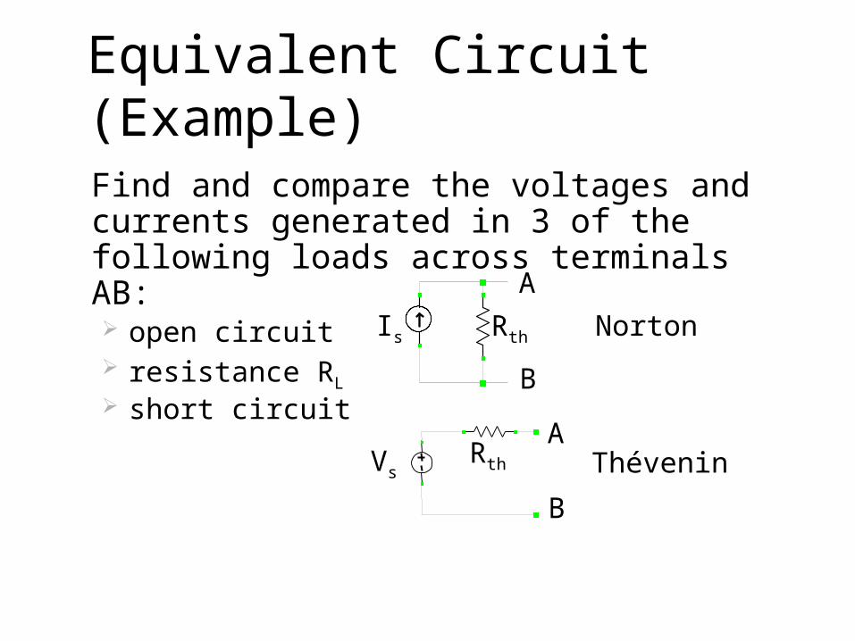
Equivalent Circuit (Example)Find and compare the voltages and currents generated in 3 of the following loads across terminals AB: open circuit resistance RL

short circuit

Rth

Vs

Is

Rth

A

A

B

B

Thévenin

Norton

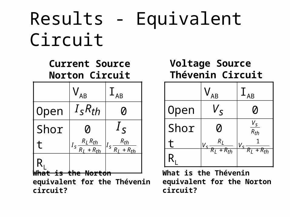
Results - Equivalent Circuit

VAB IAB

Open 0

Short 0

RL

thsRI

sI

thL

thLs RR

RRI

thL

ths RR

RI

Current SourceNorton Circuit

VAB IAB

Open 0

Short 0

RL

sV

th

sR

V

thL

Ls RR

RV

thLs RR

V1

Voltage SourceThévenin Circuit

What is the Norton equivalent for the Thévenin circuit?

What is the Thévenin equivalent for the Norton circuit?

Finding Thévenin and Norton Equivalent Circuits

Identify terminal pair at which to find the equivalent circuit.

Find voltage across the terminal pair when no load is present (open-circuit voltage Voc)

Short the terminal and find the current in the short (short-circuit current Isc)

Compute equivalent resistance as: Rth = Voc / Isc

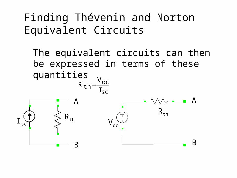
Finding Thévenin and Norton Equivalent Circuits

The equivalent circuits can then be expressed in terms of these quantities

RthIsc

A

B

Voc

Rth

A

B

sc

octh I

VR

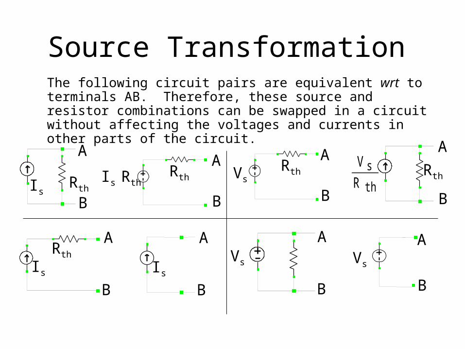
Source TransformationThe following circuit pairs are equivalent wrt to terminals AB. Therefore, these source and resistor combinations can be swapped in a circuit without affecting the voltages and currents in other parts of the circuit.

RthIs

A

B

Is RthRth

A

B

Vs Rth

A

B

Rth

A

Bth

sR

V

Is

Rth

A

B

Vs

A

B

Vs

A

B

A

B

Is

Source Transformation

Some equivalent circuits can be determined by transforming source and resistor combinations and combining parallel and serial elements around a terminal of interest.

This method can work well for simple circuits with source-resistor combinations as shown on the previous slide.

This method cannot be used if dependent sources are present.

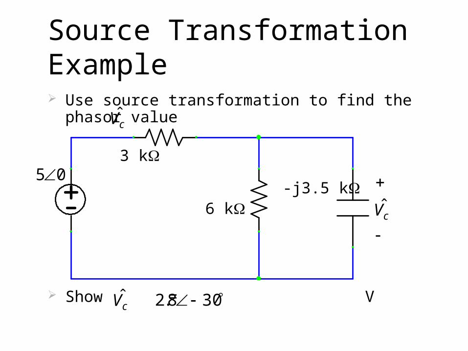
Source Transformation Example Use source transformation to find the phasor

value

Show = V

cV̂

cV̂

3 k

6 k-j3.5 k

05

cV̂ 308.2

Nodal Analysis

Identify and label all nodes in the system.

Select one node as a reference node (V=0).

Perform KCL at each node with an unknown voltage, expressing each branch current in terms of node voltages. (Exception) If branch contains a voltage source

One way: Make reference node the negative end of the voltage source and set node values on the positive end equal to the source values (reduces number of equations and unknowns by one)

Another way: (Super node) Create an equation where the difference between the node voltages on either end of the source is equal to the source value, and then use a surface around both nodes for KCL equation.

Example

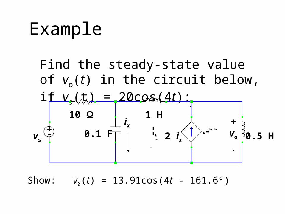
Find the steady-state value of vo(t) in the circuit below, if vs(t) = 20cos(4t):

vs

10

2 ix

1 H

0.5 H0.1 Fix

Show: v0(t) = 13.91cos(4t - 161.6º)

+vo

-

Loop/Mesh Analysis

Create loop current labels that include every circuit branch where each loop contains a unique branch (not included by any other loop) and no loops “crisscross” each other (but they can overlap in common branches).

Perform KVL around each loop expressing all voltages in terms of loop currents. If any branch contains a current source,

One way: Let only one loop current pass through source so loop current equals the source value (reduces number of equations and unknowns by one)

Another way: Let more than one loop pass through source and set combination of loop currents equal to source value (this provides an extra equation, which was lost because of the unknown voltage drop on current source)

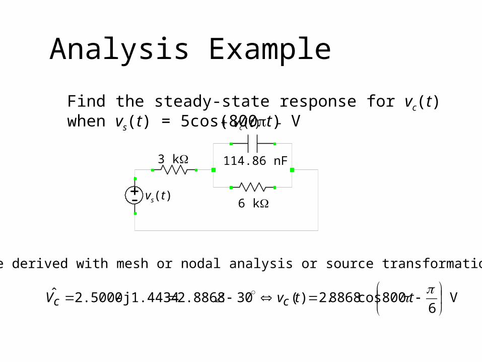
Analysis Example

Find the steady-state response for vc(t) when vs(t) = 5cos(800t) V

Can be derived with mesh or nodal analysis or source transformation:

V 6

800cos8868.2)( 302.8868 j1.4434 - 2.5000 ˆ

ttvV cc

114.86 nF

6 kW

3 kW

vs(t)

+ vc(t) -

Linearity and Superposition If a linear circuit has multiple independent sources,

then a voltage or current anywhere in the circuit is the sum of the quantities produced by the individual sources (i.e. activate one source at a time). This property is called superposition.

To deactivate a voltage source, set the voltage equal to zero (equivalent to replacing it with a short circuit).

To deactivate a current source, set the current equal to zero (equivalent to replacing it with an open circuit).

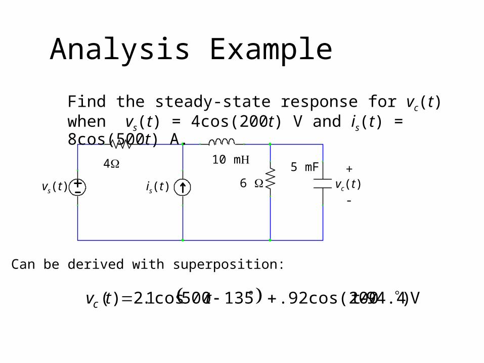
Analysis Example

Find the steady-state response for vc(t) when vs(t) = 4cos(200t) V and is(t) = 8cos(500t) A.

Can be derived with superposition:

V )94.4-t.92cos(200 135500cos1.2)( ttvc

5 mF6 W

4W

vs(t)

+vc(t)

-

10 mH

is(t)

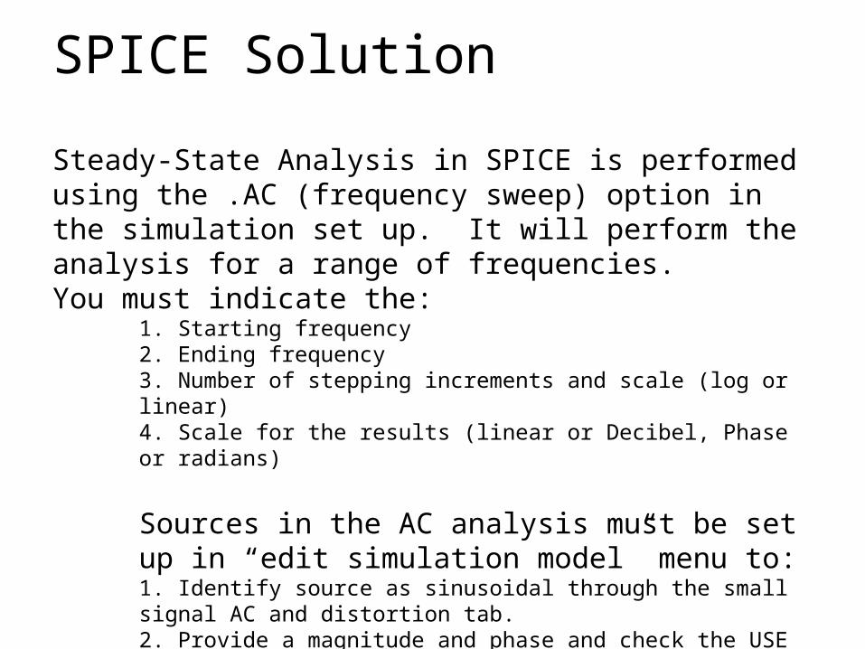
SPICE Solution

Steady-State Analysis in SPICE is performed using the .AC (frequency sweep) option in the simulation set up. It will perform the analysis for a range of frequencies.You must indicate the:

1. Starting frequency2. Ending frequency3. Number of stepping increments and scale (log or linear)4. Scale for the results (linear or Decibel, Phase or radians)

Sources in the AC analysis must be set up in “edit simulation model” menu to:1. Identify source as sinusoidal through the small signal AC and distortion tab.2. Provide a magnitude and phase and check the USE box

ex16-Small Signal AC-2-TableFREQ MAG(V(IVM)) PH_DEG(V(IVM))(Hz) (V) (deg)+100.000 +3.299 -8.213+200.000 +3.203 -16.102+300.000 +3.059 -23.413+400.000 +2.887 -30.000+500.000 +2.703 -35.817+600.000 +2.520 -40.893+700.000 +2.345 -45.295+800.000 +2.182 -49.107+900.000 +2.033 -52.411+1.000k +1.898 -55.285

SPICE Example

Find the phasor for vc(t) for vs(t)= 5cos(2ft) V in the circuit below for f = 100, 200, 300, 400, 500, …..1000 Hz. Note that 400 Hz was the frequency of the original example problem.

V R2 6k

R1 3k

IVm

C114.86n

Plotting Frequency Sweep Results

Choices for AC (frequency sweep simulation) For frequency ranges that include several

orders of magnitude, a logarithmic or Decade (DEC) scale is more practical than a linear scale

The magnitude results can also be computed on a logarithmic scale referred to a decibels or dB defined as: )(log20 10 MM dB

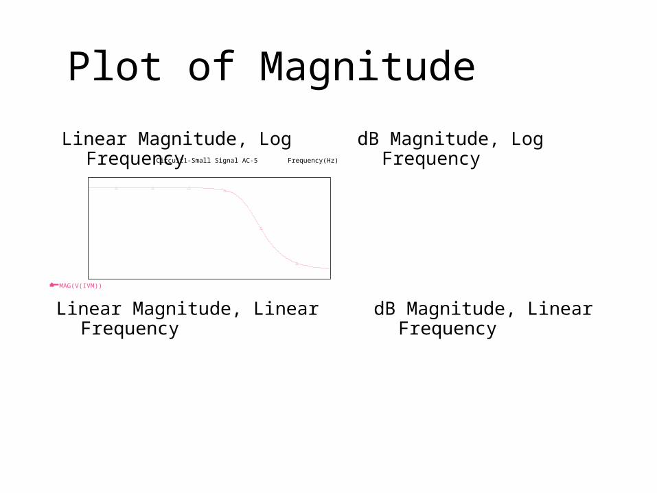
Plot of Magnitude

Linear Magnitude, Linear Frequency

dB Magnitude, Log FrequencyLinear Magnitude, Log Frequency

dB Magnitude, Linear Frequency

MAG(V(IVM))

Frequency (Hz)Circuit1-Small Signal AC-5

+0.000e+000

+1.000

+2.000

+3.000

+1.000 +10.000 +100.000 +1.000k +10.000k

DB(V(IVM))

Frequency (Hz)Circuit1-Small Signal AC-6

-20.000

+0.000e+000

+1.000 +10.000 +100.000 +1.000k +10.000k

MAG(V(IVM))

Frequency (Hz)u14ex1.ckt-Small Signal AC-7

+0.000e+000

+1.000

+2.000

+3.000

+10.000k +20.000k +30.000k +40.000k +50.000k

DB(V(IVM))

Frequency (Hz)u14ex1.ckt-Small Signal AC-8

-20.000

+0.000e+000

+10.000k +20.000k +30.000k +40.000k +50.000k

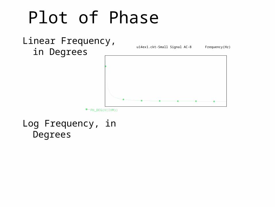
Plot of PhaseLinear Frequency, in Degrees

Log Frequency, in Degrees

PH_DEG(V(IVM))

Frequency (Hz)u14ex1.ckt-Small Signal AC-8

-50.000

+0.000e+000

+10.000k +20.000k +30.000k +40.000k +50.000k

PH_DEG(V(IVM))

Frequency (Hz)u14ex1.ckt-Small Signal AC-9

-50.000

+0.000e+000

+1.000 +10.000 +100.000 +1.000k +10.000k

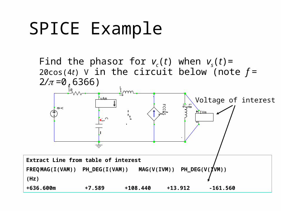
SPICE Example

Find the phasor for vc(t) when vs(t)= 20cos(4t) V in the circuit below (note f = 2/ =0.6366)

Extract Line from table of interest

FREQ MAG(I(VAM)) PH_DEG(I(VAM)) MAG(V(IVM)) PH_DEG(V(IVM))

(Hz)

+636.600m +7.589 +108.440 +13.912 -161.560

V0

R 10

L1

L0

.5

C.1

FC

CC

S

vAm

IVm

Voltage of interest