city college of new york 1 prof. jizhong xiao department of electrical engineering cuny city college...
Post on 19-Dec-2015
227 views
TRANSCRIPT

City College of New York
1
Prof. Jizhong Xiao
Department of Electrical Engineering
CUNY City College
Syllabus/Introduction/Review
Advanced Mobile Robotics

City College of New York
2
Outline
• Syllabus – Course Description– Prerequisite, Expected Outcomes– Primary Topics– Textbook and references– Grading, Office hours and contact
• How to … – How to read a research paper– How to write a reading report
• G5501 Review– What is a Robot?– Why use Robots?– Mobile Robotics

City College of New York
3
SyllabusCourse Description • This course is an in depth study of state-of-the-
art technologies and methods of mobile robotics. • The course consists of two components: lectures
on theory, and course projects. • Lectures will draw from textbooks and current
research literature with several reading discussion classes.
• In project component of this class, students are required to conduct simulation study to implement, evaluate SLAM algorithms.

City College of New York
4
Primary Topics• Mobile Robotics Review
– Locomotion/Motion Planning/Mapping– Odometry errors
• Probabilistic Robotics– Mathematic Background, Bayes Filters
• Kalman Filters (KF, EKF, UKF)• Particle Filters• SLAM (simultaneous localization and mapping)• Data Association Problems
Syllabus

City College of New York
5
SyllabusTextbooks: • Probabilistic ROBOTICS, Sebastian Thrun, Wolfram Burgard, Dieter
Fox, The MIT Press, 2005, ISBN 0-262-20162-3. Available at CCNY Book Store Reference Material:• Introduction to AI Robotics, Robin R. Murphy, The MIT Press, 2000,
ISBN 0-262-13383-0.• Introduction to Autonomous Mobile Robots, Roland Siegwart, Illah
R. Nourbakhsh, The MIT Press, 2004, ISBN 0-262-19502-X• Computational Principles of Mobile Robotics, Gregory Dudek,
Michael Jenkin, Cambridge University Press, 2000, ISBN 0-521-56876-5
• Papers from research literature
City College of New York
6
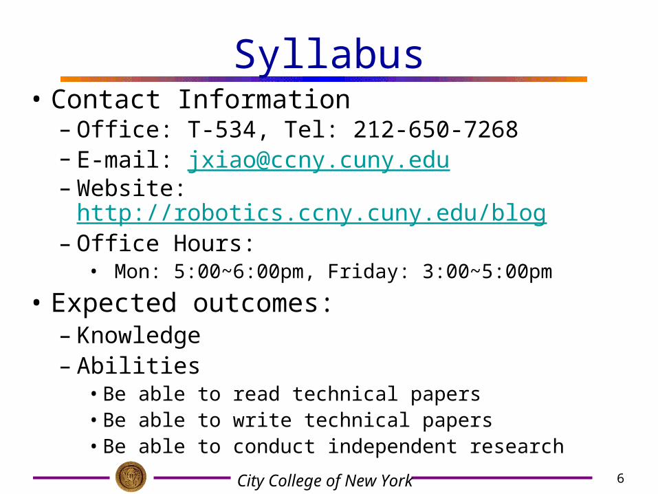
Syllabus• Contact Information
– Office: T-534, Tel: 212-650-7268– E-mail: [email protected]– Website: http://robotics.ccny.cuny.edu/blog– Office Hours:
• Mon: 5:00~6:00pm, Friday: 3:00~5:00pm
• Expected outcomes:– Knowledge– Abilities
• Be able to read technical papers• Be able to write technical papers• Be able to conduct independent research

City College of New York
7
• How to … – How to read a research paper
• Conference papers (ICRA, IROS)• Journal papers
– IEEE Transactions on Robotics– Autonomous Robots– International Journal of Robotics Research
CCNY resource:
http://www.ccny.cuny.edu/library/Menu.html
IEEE Xplorer– How to write a reading report

City College of New York
8
G5501 Course Review
City College of New York
9
Prof. Jizhong Xiao
Department of Electrical Engineering
CUNY City College
Mobile Robotics Locomotion/Motion Planning/Mapping
City College of New York
10
Contents• Review• Classification of wheels
– Fixed wheel, Centered orientable wheel, Off-centered orientable wheel, Swedish wheel
• Mobile Robot Locomotion– Differential Drive, Tricycle, Synchronous
Drive, Omni-directional, Ackerman Steering• Motion Planning Methods
– Roadmap Approaches (Visibility graphs, Voronoi diagram)
– Cell Decomposition (Trapezoidal Decomposition, Quadtree Decomposition)
– Potential Fields
• Mapping and Localization

City College of New York
11
Review• What are Robots?
– Machines with sensing, intelligence and mobility (NSF)
• To qualify as a robot, a machine must be able to: 1) Sensing and perception: get information from its surroundings 2) Carry out different tasks: Locomotion or manipulation, do
something physical–such as move or manipulate objects3) Re-programmable: can do different things4) Function autonomously and/or interact with human beings
• Why use Robots?– Perform 4A tasks in 4D environments
4A: Automation, Augmentation, Assistance, Autonomous
4D: Dangerous, Dirty, Dull, Difficult

City College of New York
12
Review
• Robot Manipulator– Kinematics – Dynamics– Control
• Mobile Robot – Kinematics/Control – Sensing and Sensors– Motion planning – Mapping/Localization
x
yz
x
yz
x
yz
x
z
y

City College of New York
13
Mobile Robot Examples
ActivMedia Pioneer II Sojourner Rover
NASA and JPL, Mars exploration

City College of New York
14
Wheeled Mobile Robots
• Locomotion — the process of causing an robot to move.– In order to produce motion, forces must be applied to the robot– Motor output, payload
• Kinematics – study of the mathematics of motion without considering the forces that affect the motion.– Deals with the geometric relationships that govern the system– Deals with the relationship between control parameters and the
behavior of a system.
• Dynamics – study of motion in which these forces are modeled– Deals with the relationship between force and motions.

City College of New York
15
Notation
Posture: position(x, y) and orientation

City College of New York
16
Wheels
Lateral slip
Rolling motion

City College of New York
17
Wheel TypesFixed wheel Centered orientable wheel
Off-centered orientable wheel (Castor wheel) Swedish wheel:omnidirectional
property
City College of New York
18
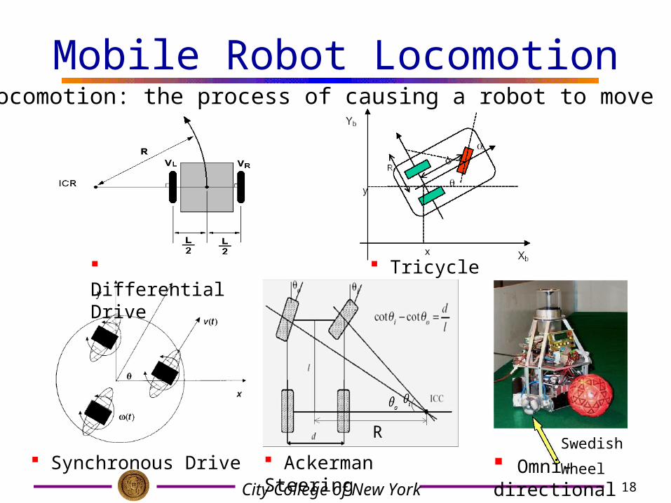
Mobile Robot Locomotion
Swedish Wheel
Locomotion: the process of causing a robot to move
Tricycle
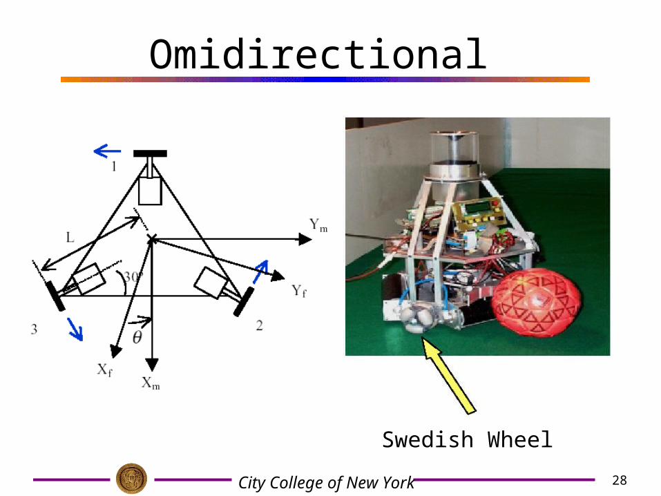
Synchronous Drive Omni-directional
Differential Drive
R
Ackerman Steering

City College of New York
19
• Posture of the robot
v : Linear velocity of the robot
w : Angular velocity of the robot
(notice: not for each wheel)
(x,y) : Position of the robot
: Orientation of the robot
• Control input
Differential Drive

City College of New York
20
Differential Drive – linear velocity of right wheel – linear velocity of left wheelr – nominal radius of each wheelR – instantaneous curvature radius (ICR) of the robot trajectory (distance from ICC to the midpoint between the two wheels).
Property: At each time instant, the left and right wheels must follow a trajectory that moves around the ICC at the same angular rate , i.e.,
RVL
R )2
( LVL
R )2
(
)(tVR
)(tVL

City College of New York
21
Differential Drive
0cossincossin
yx
y
x
• Nonholonomic Constraint
90
Property: At each time instant, the left and right wheels must follow a trajectory that moves around the ICR at the same angular rate , i.e.,
RVL
R )2
( LVL
R )2
(
• Kinematic equation
Physical Meaning?

City College of New York
22
Non-holonomic constraint
So what does that mean?Your robot can move in some directions (forward
and backward), but not others (sideward).
The robot can instantlymove forward and backward, but can not move sideward
Parallel parking,Series of maneuvers
A non-holonomic constraint is a constraint on the feasible velocities of a body

City College of New York
23
Differential Drive• Basic Motion Control
• Straight motion R = Infinity VR =
VL
• Rotational motion R = 0 VR =
-VL
R : Radius of rotation
Instantaneous center of curvature (ICC)

City College of New York
24
• Velocity Profile
: Radius of rotation
: Length of path : Angle of
rotation
3 1 0 2
3 1 0 2
Differential Drive

City College of New York
25
Tricycle
d: distance from the front wheel to the rear axle
• Steering and power are provided through the front wheel
• control variables:– angular velocity of steering wheel ws(t)
– steering direction α(t)

City College of New York
26
Tricycle Kinematics model in the world frame---Posture kinematics model

City College of New York
27
Synchronous Drive
• All the wheels turn in unison– All wheels point in the
same direction and turn at the same rate
– Two independent motors, one rolls all wheels forward, one rotate them for turning
• Control variables (independent)– v(t), ω(t)
City College of New York
28
Omidirectional
Swedish Wheel
City College of New York
29
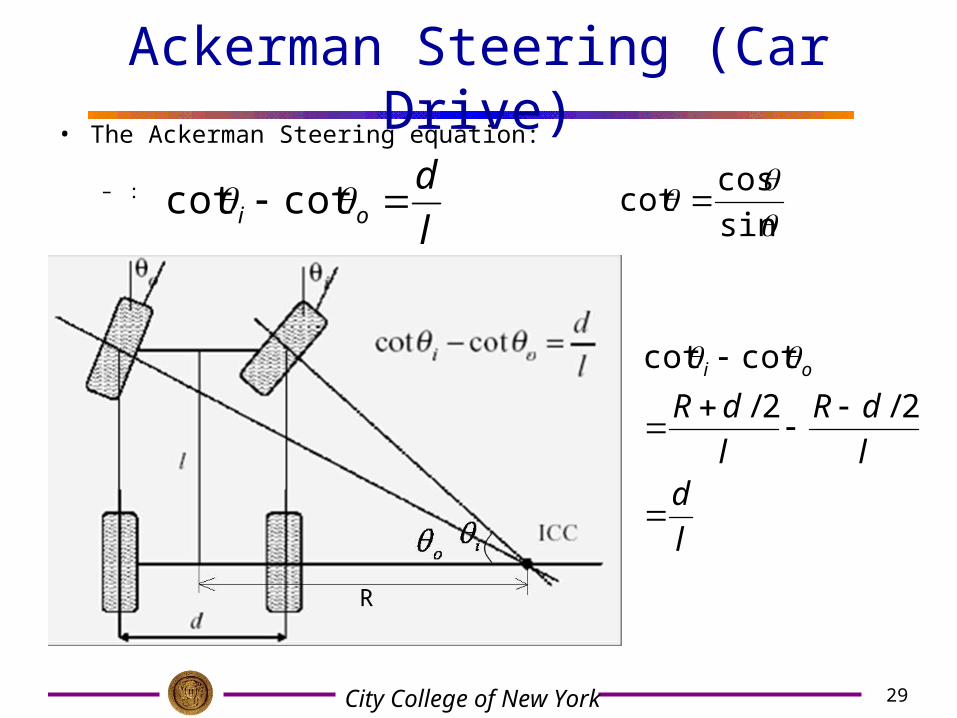
Ackerman Steering (Car Drive)• The Ackerman Steering equation:
– :
sin
coscot
l
dl
dR
l
dRoi
2/2/
cotcot
l
doi cotcot
R
City College of New York
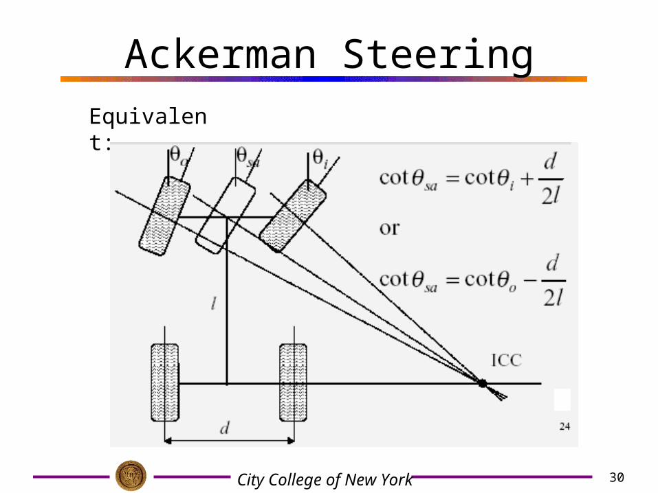
30
Ackerman SteeringEquivalent:

City College of New York
31
Car-like Robot
1uR
2
1
1
1
tan
sin
cos
ul
u
uy
ux
0cossin yx non-holonomic constraint:
: forward velocity of the rear wheels
: angular velocity of the steering wheels
1u
2u
l : length between the front and rear wheels
X
Y
yx,
l
ICC
R
1tanu
l
Rear wheel drive car model:
Driving type: Rear wheel drive, front wheel steering
City College of New York
32
Robot Sensing • Collect information about the world• Sensor - an electrical/mechanical/chemical device
that maps an environmental attribute to a quantitative measurement
• Each sensor is based on a transduction principle - conversion of energy from one form to another
• Extend ranges and modalities of Human Sensing

City College of New York
33
Electromagnetic SpectrumElectromagnetic SpectrumVisible Spectrum
700 nm 400 nm
City College of New York
34
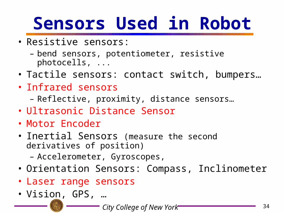
Sensors Used in Robot• Resistive sensors:
– bend sensors, potentiometer, resistive photocells, ...
• Tactile sensors: contact switch, bumpers…• Infrared sensors
– Reflective, proximity, distance sensors…
• Ultrasonic Distance Sensor• Motor Encoder• Inertial Sensors (measure the second derivatives of
position)– Accelerometer, Gyroscopes,
• Orientation Sensors: Compass, Inclinometer• Laser range sensors• Vision, GPS, …

City College of New York
35
Mobot System Overview
Abstraction level
Motor Modeling: what voltage should I set now ?
Control (PID): what voltage should I set over time ?
Kinematics: if I move this motor somehow, what happens in other coordinate systems ?
Motion Planning: Given a known world and a cooperative mechanism, how do I get there from here ?
Bug Algorithms: Given an unknowable world but a known goal and local
sensing, how can I get there from here?
Mapping: Given sensors, how do I create a useful map?
low-level
high-level
Localization: Given sensors and a map, where am I ?Vision: If my sensors are eyes, what do I do?

City College of New York
36
What is Motion Planning?
• Determining where to go without hit obstacles

City College of New York
37
References• G. Dudek, M. Jenkin, Computational Principles of Mobile Robots, MIT Press, 2000 (Chapter 5)• J.C. Latombe, Robot Motion Planning, Kluwer Academic Publishers, 1991.
• Additional references – Path Planning with A* algorithm
• S. Kambhampati, L. Davis, “Multiresolution Path Planning for Mobile Robots”, IEEE Journal of Robotrics and Automation,Vol. RA-2, No.3, 1986, pp.135-145.
– Potential Field • O. Khatib, “Real-Time Obstacle Avoidance for Manipulators and
Mobile Robots”, Int. Journal of Robotics Research, 5(1), pp.90-98, 1986.
• P. Khosla, R. Volpe, “Superquadratic Artificial Potentials for Obstacle Avoidance and Approach” Proc. Of ICRA, 1988, pp.1178-1784.
• B. Krogh, “A Generalized Potential Field Approach to Obstacle Avoidance Control” SME Paper MS84-484.
City College of New York
38
Motion Planning
– Configuration Space– Motion Planning Methods
• Roadmap Approaches• Cell Decomposition• Potential Fields
Motion Planning: Find a path connecting an initial configuration to goal configuration without collision with obstacles
Assuming the environment is known!
City College of New York
39
The World consists of...
• Obstacles– Already occupied spaces of the world– In other words, robots can’t go there
• Free Space– Unoccupied space within the world– Robots “might” be able to go here– To determine where a robot can go, we need to
discuss what a Configuration Space is

City College of New York
40
Configuration Space
Configuration Space is the space of all possible robot configurations.
Notation:
A: single rigid object –(the robot)
W: Euclidean space where A moves;
B1,…Bm: fixed rigid obstacles distributed in W
32 RorRW
• FW – world frame (fixed frame)• FA – robot frame (moving frame rigidly associated with the robot)
Configuration q of A is a specification of the physical state (position and orientation) of A w.r.t. a fixed environmental frame FW.

City College of New York
41
Configuration Space
For a point robot moving in 2-D plane, C-space is
Configuration Space of A is the space (C )of all possible configurations of A.
qslug
qrobot
CCfree
Cobs
2R
Point robot (free-flying, no constraints)

City College of New York
42
Configuration Space
For a point robot moving in 3-D, the C-space is
x
y
qstart
qgoal
C
Cfree
Cobs
3R
What is the difference between Euclidean space and C-space?

City College of New York
43
Configuration Space
X
Y
A robot which can translate in the plane
X
Y A robot which can translate and rotate in the plane
x
Y
C-space:
C-space:
2-D (x, y)
3-D (x, y, )
Euclidean space: 2R

City College of New York
44
Configuration Space
2R manipulator
topology
Configuration space

City College of New York
45
Configuration Space
Two points in the robot’s workspace
270
360
180
90
090 18013545
Torus(wraps horizontally and vertically)
qrobot
qslug
City College of New York
46
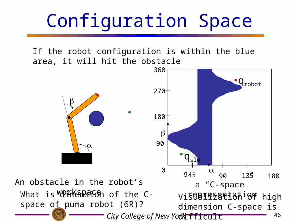
Configuration Space
An obstacle in the robot’s workspace
270
360
180
90
090 18013545
qslug
qrobot
a “C-space” representation
If the robot configuration is within the blue area, it will hit the obstacle
What is dimension of the C-space of puma robot (6R)?
Visualization of high dimension C-space is difficult

City College of New York
47
Motion Planning Revisit
Find a collision free path from an initial configuration to goal configuration while taking into account the constrains (geometric, physical, temporal)
A separate problem for each robot?
C-space concept provide a generalized framework to study the motion planning problem

City College of New York
48
What if the robot is not a point?
The Pioneer-II robot should probably not be modeled as a point...

City College of New York
49
What if the robot is not a point?
Expand obstacle(s)
Reduce robot
not quite right ...

City College of New York
50
Obstacles Configuration SpaceC-obstacle
Point robot

City College of New York
51
C-obstacle in 3-DWhat would the configuration space of a 3DOF rectangular robot (red) in this world look like?
(The obstacle is blue.)
x
y
0º
180º
can we stay in 2d ?
3-D

City College of New York
52
One sliceTaking one slice of the C-obstacle in which the robot is rotated 45 degrees...
x
y45 degrees
How many slices does P R have?
P
RP R
City College of New York
53
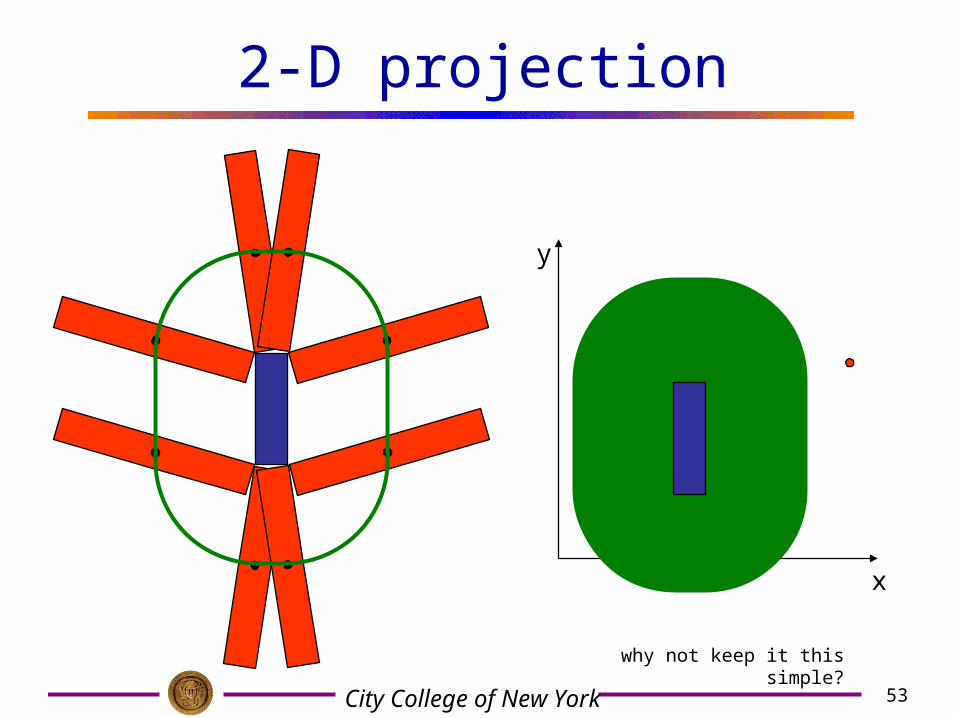
2-D projection
why not keep it this simple?
x
y

City College of New York
54
Projection problems
qinit
qgoal too conservative!

City College of New York
55
Motion Planning Methods
Roadmap approaches• Visibility Graph
• Voronoi Diagram
Cell decomposition
• Trapezoidal decomposition
• Quadtree decomposition
Potential Fields
Full-knowledge motion planning

City College of New York
56
Full-knowledge motion planning
approximate free space
represented via a quadtree
Cell decompositionsRoadmaps
exact free space
represented via convex polygons
visibility graph
voronoi diagram

City College of New York
57
Roadmap: Visibility GraphsVisibility graphs: In a polygonal (or polyhedral) configuration space, construct all of the line segments that connect vertices to one another (and that do not intersect the obstacles themselves).
From Cfree, a graph is defined
Converts the problem into graph search.
Dijkstra’s algorithmO(N^2)
N = the number of vertices in C-space
Formed by connecting all “visible” vertices, the start point and the end point, to each other.For two points to be “visible” no obstacle can exist between them
Paths exist on the perimeter of obstacles

City College of New York
58
Visibility graph drawbacks
Visibility graphs do not preserve their optimality in higher dimensions:
In addition, the paths they find are “semi-free,” i.e. in contact with obstacles.
shortest path
shortest path within the visibility graph
No clearance

City College of New York
59
“official” Voronoi diagram
(line segments make up the Voronoi diagram isolates a set of points)
Roadmap: Voronoi diagrams
Generalized Voronoi Graph (GVG): locus of points equidistant from the closest two or more obstacle boundaries, including the workspace boundary.
Property: maximizing the clearance between the points and obstacles.

City College of New York
60
Roadmap: Voronoi diagrams
• GVG is formed by paths equidistant from the two closest objects
• maximizing the clearance between the obstacles.
• This generates a very safe roadmap which avoids obstacles as much as possible

City College of New York
61
Voronoi Diagram: Metrics• Many ways to measure distance; two are:
– L1 metric• (x,y) : |x| + |y| = const
– L2 metric• (x,y) : x2 +y2 = const

City College of New York
62
Voronoi Diagram (L1)
Note the lack of curved edges

City College of New York
63
Voronoi Diagram (L2)
Note the curved edges

City College of New York
64
Motion Planning Methods
Roadmap approaches• Visibility Graph
• Voronoi Diagram
Cell decomposition
• Exact Cell Decomposition (Trapezoidal)
• Approximate Cell Decomposition (Quadtree)
Potential Fields
Hybrid local/global

City College of New York
65
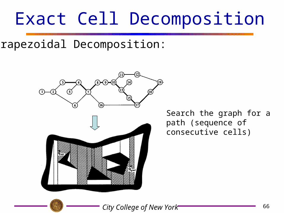
Exact Cell Decomposition
Decomposition of the free space into trapezoidal & triangular cells
Connectivity graph representing the adjacency relation between the cells
(Sweepline algorithm)
Trapezoidal Decomposition:
City College of New York
66
Exact Cell Decomposition
Search the graph for a path (sequence of consecutive cells)
Trapezoidal Decomposition:

City College of New York
67
Exact Cell Decomposition
Transform the sequence of cells into a free path (e.g., connecting the mid-points of the intersection of two consecutive cells)
Trapezoidal Decomposition:

City College of New York
68
Obtaining the minimum number of convex cells is NP-complete.
Optimality
there may be more details in the world than the task needs to worry about...
15 cells 9 cells
Trapezoidal decomposition is exact and complete, but not optimal
Trapezoidal Decomposition:

City College of New York
69
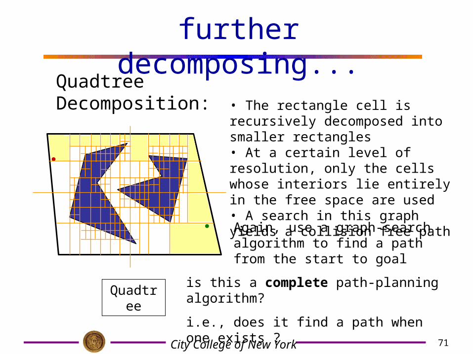
Quadtree Decomposition:
Approximate Cell Decomposition
recursively subdivides each mixed obstacle/free (sub)region into four quarters...
Quadtree:

City College of New York
70
further decomposing...
recursively subdivides each mixed obstacle/free (sub)region into four quarters...
Quadtree:
Quadtree Decomposition:
City College of New York
71
further decomposing...
Again, use a graph-search algorithm to find a path from the start to goal
Quadtreeis this a complete path-planning algorithm?
i.e., does it find a path when one exists ?
Quadtree Decomposition:• The rectangle cell is recursively decomposed into smaller rectangles• At a certain level of resolution, only the cells whose interiors lie entirely in the free space are used• A search in this graph yields a collision free path
City College of New York
72
Motion Planning Methods
Roadmap approaches
Cell decomposition
• Exact Cell Decomposition (Trapezoidal)
• Approximate Cell Decomposition (Quadtree)
Potential Fields
Hybrid local/global

City College of New York
73
Potential Field Method Potential Field (Working Principle)
– The goal location generates an attractive potential – pulling the robot towards the goal– The obstacles generate a repulsive potential – pushing the robot far away from the obstacles– The negative gradient of the total potential is treated as an artificial force applied to the robot
-- Let the sum of the forces control the robot
C-obstacles

City College of New York
74
• Compute an attractive force toward the goal
Potential Field Method
C-obstacles
Attractive potential

City College of New York
75
Potential Field Method
Repulsive Potential
Create a potential barrier around the C-obstacle region that cannot be traversed by the robot’s configuration
It is usually desirable that the repulsive potential does not affect the motion of the robot when it is sufficiently far away from C-obstacles
• Compute a repulsive force away from obstacles

City College of New York
76
• Compute a repulsive force away from obstacles
Potential Field Method
• Repulsive Potential

City College of New York
77
• Sum of Potential
Potential Field Method
C-obstacle
Attractive potential Repulsive potential
Sum of potentials
City College of New York
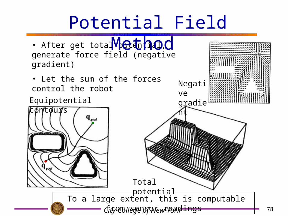
78
• After get total potential, generate force field (negative gradient)
• Let the sum of the forces control the robot
To a large extent, this is computable from sensor readings
Equipotential contours
Negative gradient
Total potential
Potential Field Method

City College of New York
79
random walks are not perfect...
Potential Field Method
• Spatial paths are not preplanned and can be generated in real time
• Planning and control are merged into one function
• Smooth paths are generated
• Planning can be coupled directly to a control algorithm
Pros:
• Trapped in local minima in the potential field
• Because of this limitation, commonly used for local path planning
• Use random walk, backtracking, etc to escape the local minima
Cons:

City College of New York
80
Motion Planning Summary• Motion Planning Methodololgies – Roadmap – Cell Decomposition – Potential Field
• Roadmap – From Cfree a graph is defined (Roadmap) – Ways to obtain the Roadmap
• Visibility graph• Voronoi diagram
• Cell Decomposition – The robot free space (Cfree) is decomposed into simple regions (cells) – The path in between two poses of a cell can be easily generated• Potential Field – The robot is treated as a particle acting under the influence of a potential field U, where: • the attraction to the goal is modeled by an additive field • obstacles are avoided by acting with a repulsive force that yields a negative field
Global methods
Local methods
City College of New York
81
Mapping/Localization
• Answering robotics’ big questions– How to get a map of an environment with
imperfect sensors (Mapping)– How a robot can tell where it is on a map
(localization)– SLAM (Simultaneous Localization and
Mapping)• It is an on-going research• It is the most difficult task for robot
– Even human will get lost in a building!

City College of New York
82
Using sonar to create maps
What should we conclude if this sonar reads 10 feet?
10 feet
there is something somewhere around here
there isn’t something here
Local Mapunoccupied
occupied
or ...
no information

City College of New York
83
Using sonar to create maps
What should we conclude if this sonar reads 10 feet...
10 feet
and how do we add the information that the next sonar reading (as the robot moves) reads 10 feet, too?
10 feet

City College of New York
84
Combining sensor readings
• The key to making accurate maps is combining lots of data.
• But combining these numbers means we have to know what they are !
What should our map contain ?
• small cells
• each represents a bit of the robot’s environment
• larger values => obstacle
• smaller values => free
what is in each cell of this sonar model / map ?

City College of New York
85
What is it a map of?
Several answers to this question have been tried:
It’s a map of occupied cells. oxy oxy cell (x,y) is occupied
cell (x,y) is unoccupied
Each cell is either occupied or unoccupied -- this was the approach taken by the Stanford Cart.
pre ‘83
What information should this map contain, given that it is created with sonar ?

City College of New York
86
Several answers to this question have been tried:
It’s a map of occupied cells.
It’s a map of probabilities: p( o | S1..i )
p( o | S1..i )
It’s a map of odds.
The certainty that a cell is occupied, given the sensor readings S1, S2, …, Si
The certainty that a cell is unoccupied, given the sensor readings S1, S2, …, Si
The odds of an event are expressed relative to the complement of that event.
odds( o | S1..i ) = p( o | S1..i )p( o | S1..i )
The odds that a cell is occupied, given the sensor readings S1, S2, …,
Si
oxy oxy cell (x,y) is occupied
cell (x,y) is unoccupied
‘83 - ‘88
pre ‘83
What is it a map of ?
probabilities
evidence = log2(odds)

City College of New York
87
An example map
units: feetEvidence grid of a tree-lined outdoor path
lighter areas: lower odds of obstacles being present
darker areas: higher odds of obstacles being presenthow to combine them?
City College of New York
88
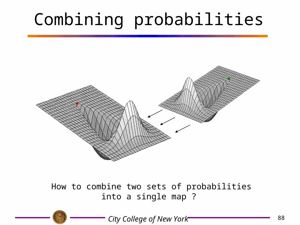
Combining probabilities
How to combine two sets of probabilities into a single map ?

City College of New York
89
Conditional probability
Some intuition...
p( o | S ) = The probability of event o, given event S .The probability that a certain cell o is occupied, given that the robot sees the sensor reading S .
p( S | o ) = The probability of event S, given event o .The probability that the robot sees the sensor reading S , given that a certain cell o is occupied.
• What is really meant by conditional probability ?
• How are these two probabilities related?
p( o | S ) = p(S | o) ??
City College of New York
90
Bayes Rule
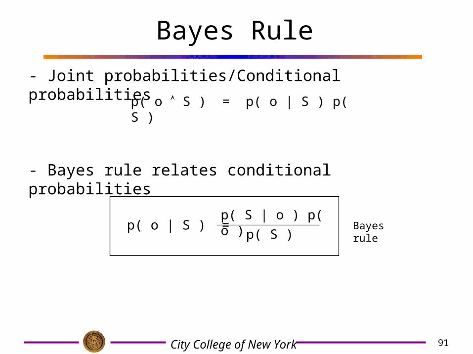
p( o S ) = p( o | S ) p( S )
- Joint probabilities/Conditional probabilities
City College of New York
91
Bayes Rule
- Bayes rule relates conditional probabilities
p( o | S ) = p( S | o ) p( o )
p( S )Bayes rule
p( o S ) = p( o | S ) p( S )
- Joint probabilities/Conditional probabilities
City College of New York
92
Bayes Rule
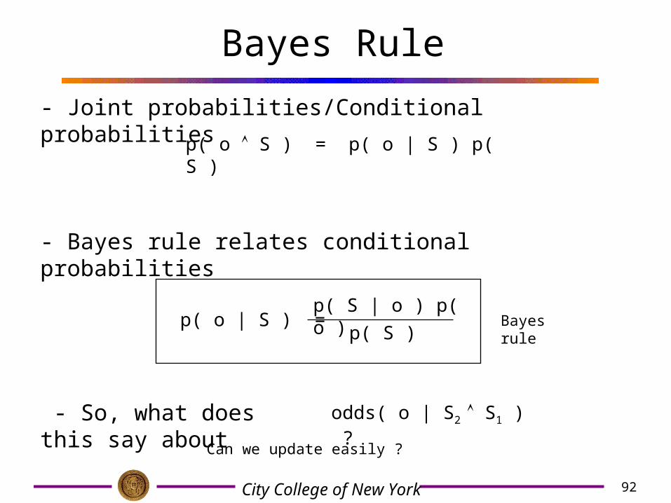
- Bayes rule relates conditional probabilities
p( o | S ) = p( S | o ) p( o )
- So, what does this say about
p( S )Bayes rule
odds( o | S2 S1 ) ?
p( o S ) = p( o | S ) p( S )
- Joint probabilities/Conditional probabilities
Can we update easily ?

City College of New York
93
Combining evidence
So, how do we combine evidence to create a map?
What we want --
odds( o | S2 S1) the new value of a cell in the map after the sonar reading S2
What we know --
odds( o | S1) the old value of a cell in the map (before sonar reading S2)
p( Si | o ) & p( Si | o ) the probabilities that a certain obstacle causes the sonar reading Si

City College of New York
94
Combining evidence
odds( o | S2 S1) = p( o | S2 S1 )
p( o | S2 S1 )
City College of New York
95
Combining evidence
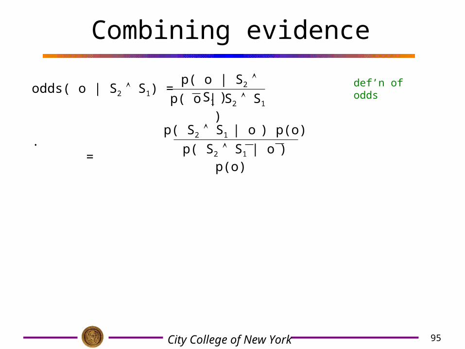
odds( o | S2 S1) = p( o | S2 S1 )
p( o | S2 S1 )
. = p( S2 S1 | o ) p(o)
p( S2 S1 | o ) p(o)
def’n of odds

City College of New York
96
p( S2 | o ) p( S1 | o ) p(o)
Combining evidence
odds( o | S2 S1) = p( o | S2 S1 )
p( o | S2 S1 )
. =
. =
p( S2 S1 | o ) p(o)
p( S2 S1 | o ) p(o)
p( S2 | o ) p( S1 | o ) p(o)
def’n of odds
Bayes’ rule (+)
City College of New York
97
p( S2 | o ) p( S1 | o ) p(o)
Combining evidence
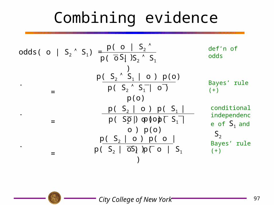
odds( o | S2 S1) = p( o | S2 S1 )
p( o | S2 S1 )
. =
. =
. =
p( S2 S1 | o ) p(o)
p( S2 S1 | o ) p(o)
p( S2 | o ) p( S1 | o ) p(o)
def’n of odds
Bayes’ rule (+)
conditional independence of S1 and
S2
p( S2 | o ) p( o | S1 )p( S2 | o ) p( o | S1 ) Bayes’ rule
(+)
City College of New York
98
p( S2 | o ) p( S1 | o ) p(o)
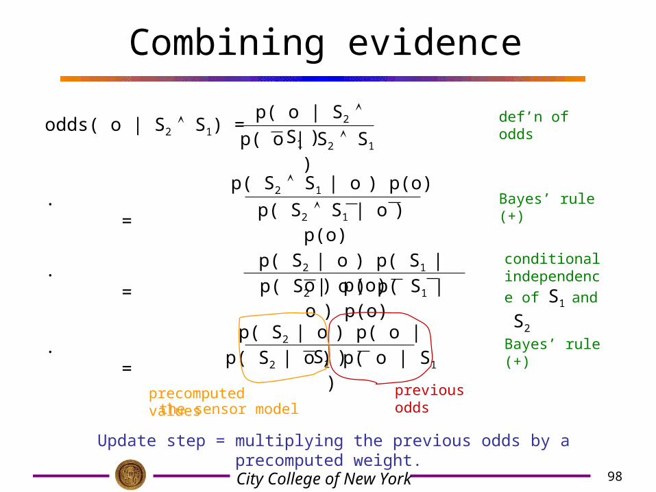
Combining evidence
odds( o | S2 S1) = p( o | S2 S1 )
p( o | S2 S1 )
. =
. =
. =
p( S2 S1 | o ) p(o)
p( S2 S1 | o ) p(o)
p( S2 | o ) p( S1 | o ) p(o)
Update step = multiplying the previous odds by a precomputed weight.
def’n of odds
Bayes’ rule (+)
conditional independence of S1 and
S2
p( S2 | o ) p( o | S1 )p( S2 | o ) p( o | S1 ) Bayes’ rule
(+)
previous oddsprecomputed valuesthe sensor model

City College of New York
99
represent space as a collection of cells, each with the odds (or probability) that it contains an obstacle
Lab environment
not surelikely obstacle
likely free space
Evidence Grids...
evidence = log2(odds)
Mapping Using Evidence Grids
lighter areas: lower evidence of obstacles being presentdarker areas: higher evidence of obstacles being present

City College of New York
100
Localization Methods• Markov Localization:
– Represent the robot’s belief by a probability distribution over possible positions and uses Bayes’ rule and convolution to update the belief whenever the robot senses or moves
• Monte-Carlo methods
• Kalman Filtering
• SLAM (simultaneous localization and mapping)• ….

City College of New York
101
Class Schedule
Homework 1 posted on the web.

City College of New York
102
Thank you!