CLARREO Langley IR Study:Numerical simulation

Bruce Wielicki1, Seiji Kato1, Fred Rose2,

Dave Kratz1, Xu Liu1, Sunny San-Mack2,

and Walt Miller2

1NASA Langley Research Center2Science Systems & Applications Inc.

the First CLARREO Mission Study Team MeetingNewport News, Virginia

April 30 to May 2, 2008

Ties to Traceability Matrix

• Climate model OSSEs Optimal for studies related to impact of benchmark spectra on climate change detection, attribution, prediction accuracy, decade to 100 year time scales, clear vs all-sky simulations

• Observation + RTM spectra simulations Optimal for studies of field of view (spatial variability < 100km scale), realistic interannual variability, realistic clouds, aerosols (e.g. A-train), issues of sampling/swath for a range of time/space scales, diurnal sampling studies.

Ties to Traceability Matrix

• LaRC IR Studies Summary:– A-train + RTM for most realistic aerosol/cloud variability

• Field of View, Cirrus + Trade Cu effects, Cloud Overlap, Spectral Coverage (e.g. Far-IR)

– Line-by-Line studies of linearity of distributions of atmospheric properties to averaged spectra

• Benchmark spectra relation to underlying climate signals

– Intercalibration of broadband and imagers in solar and infrared (last workshop).

• Field of view, Swath, Orbit, Pointing ability, knowledge, control

– Full Swath vs Nadir Only Sampling using CERES surface, cloud, aerosol, radiation data.

• Swath, Number of Orbits

– Diurnal Sampling studies for climate change: CERES + 3-hrly geo data, vs CERES Terra 1030LT only

• Orbits, Number of Orbits

Method

• Step 1: Use simple clouds and atmosphere and a) test sensitivity of the TOA effective temperature (spectrum) to atmospheric and cloud properties b) test if we can infer atmospheric property changes from time series of spectrum anomalies.

• Step 2: Use A-train realistic cloud fields, test our results from Approach 1.

Realistic Cloud fields

• Cloud fields are derived from CALIPSO, CloudSat, and MODIS (C3M), including thin cirrus, boundary layer cumulus, multi-layer clouds, and aerosols.

• C3M product contains merged CALIPSO, CloudSat, CERES and MODIS data, SW and LW TOA flux from CERES, and flux profiles computed with CALIPSO, CloudSat, and MODIS clouds and aerosols (work is funded by NASA Energy Water Cycle Study (NEWS)

A-train

1 km

333 m

MODIS Pixel Calipso Shots

MODIS Swath

1.4 km

CloudSat Profile

1.1 km

CALIPSO CloudSat MODIS collocation

From S. Sun-Mack

CALIPSO CloudSat MODIS merging with CERES

Merged clouds

Cloud and aerosol fields

from 532 nm

Cloud cover over CALIPSO-CloudSat ground-track

2.7% 6.1%

11.2% 15.0%

Clear-sky

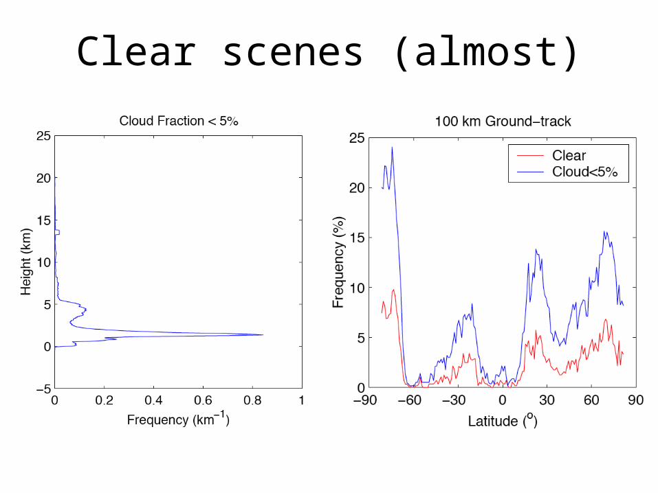
Clear scenes (almost)

Study with CALIPSO-CloudSat cloud fields

• Compute TOA spectra with MODTRAN, Principal Component Radiative Transfer Model (PCRTM), and lbl code.

• Examine whether or not atmospheric property changes can be detected from TOA spectra.

• Examine whether or not signals can be separated when more than one variables change at the same time.

Study with simple cloud fields

Averaging spectral data

• Which atmospheric variables give a linear response to the brightness temperature at TOA?

• Look for the mean spectra = spectrum of the mean

• How does the linearity depend on the mean atmospheric state?

€

I(x) ≈ I(x)

Hypothetical atmospheric property change

• Assume a distribution of a cloud or an atmospheric property x at time t1.

• Perturb the distribution for the distribution of x at time t2.• Compute mean spectrum from the distribution at t1 and t2

separately by weighting the spectrum by frequency of occurrence.

• Compute the difference of the mean spectrum at t1 and t2:

• Compute the mean of x at t1 and t2, two spectra using two

mean values, and the difference €

ΔT(λ ) ← ΔI(λ ) = I(t2,x2,λ ) − I(t1,x1,λ )

€

ΔTm (λ ) ← ΔIm (λ ) = I(t2,x2,λ ) − I(t1,x1,λ )

Simple study with MODTRAN

€

ΔTm ← ΔIm (λ ) = I(t2,x2,λ ) − I(t1,x1,λ )

€

ΔT(λ ) ← ΔI(λ ) = I(t2,x2,λ ) − I(t1,x1,λ )Black

Blue

€

ΔTm (λ ) − ΔT(λ )Orange

Mean0.981.01

€

ΔTm ← ΔIm (λ ) = I(t2,x2,λ ) − I(t1,x1,λ )

€

ΔT(λ ) ← ΔI(λ ) = I(t2,x2,λ ) − I(t1,x1,λ )Black

Blue

€

ΔTm (λ ) − ΔT(λ )Orange

Mean10 km12 km

Sensitivity

Cloud heightEmissivity = 1-exp(-tau*0.5)Water vapor Scale heightLapse rate (0 - 15 km) --> T(z)Skin temperatureSurface air temperature (fixed QSH, RHSFC) -->H2O(z)Surface relative humidity (fixed QSH, TSFC) -->H2O(z)

Linearity

Cloud emissivity 0.4+-0.01 Surface skin temp. 300+-1K

Cloud height 10+-1 km Surface air temp. 300+-5K

Langley LW Line by Line Modeling

Strategy

• Use LBL code to validate MODTRAN and PCRTM (especially spectra with clouds).

• MODTRAN and PCRTM run faster than LBL. PCRTM is more flexible with inputs.

Diurnal Cycles: Full 3-hourly vs Terra 1030LT onlyDiurnal Cycles: Full 3-hourly vs Terra 1030LT only

Is interannual variability in regional, zonal, and Is interannual variability in regional, zonal, and global fluxes captured accurately by just Terra global fluxes captured accurately by just Terra

1030LT vs full 3-hourly data?1030LT vs full 3-hourly data?

How do the differences compare to expected How do the differences compare to expected climate forcing and response?climate forcing and response?

GEO = CERES + GEO = 3-hourly DataGEO = CERES + GEO = 3-hourly DataNon-GEO = CERES Terra only = 1030 AM/PM onlyNon-GEO = CERES Terra only = 1030 AM/PM only

Tropical and Global Mean Effect of Diurnal Cycle: Very Small

GEO is CERES + 3-hourly Geo Diurnal Cycle, nonGEO = CERES Terra Only

Tropical and Global Mean Effect of Diurnal Cycle: Very Small

GEO is CERES + 3-hourly Geo Diurnal Cycle, nonGEO = CERES Terra Only

Jan 2001 De-seasonalized SW Flux Anomaly Relative to 2001-2005 Avg

(CERES Terra plus 3-hourly geostationary data for diurnal cycle)

Jan 2001 De-seasonalized SW Flux Anomaly Relative to 2001-2005 Avg

(CERES Terra (1030LT) only for diurnal cycle)

Jan 2001 De-seasonalized SW Flux Anomaly Relative to 2001-2005 Avg

(With and Without Geo: Effect of Diurnal Cycle is Small)

Jan 2001 De-seasonalized LW Flux Anomaly Relative to 2001-2005 Avg

(CERES Terra plus 3-hourly geostationary data for diurnal cycle)

Jan 2001 De-seasonalized LW Flux Anomaly Relative to 2001-2005 Avg

(CERES Terra (1030LT) only for diurnal cycle)

Jan 2001 De-seasonalized LW Flux Anomaly Relative to 2001-2005 Avg

(With and Without Geo: Effect of Diurnal Cycle is Small)

50

Conclusions

• Regional, Zonal, Global monthly and interannual variations of SW and LW fluxes examined

• Compared 3-hourly vs Terra sunsynch 1030LT only • Used all-sky fluxes to include both clear and cloudy

diurnal cycles (land, stratus, convection, desert, etc)• While regional differences can be large in the mean

fields (“true” vs 1030LT), global differences are very small.

• For anomalies (monthly, interannual, regional, zonal, global) “true” vs 1030LT showed very small differences, with the solar flux effects about 3 times as large as infrared

• LW and SW anomalies from “true” vs 1030LT anomalies are much less than natural variability

51

Conclusions

• These tests should be repeated in climate model OSSEs for CLARREO spectral radiances

• Extend trends from global to zonal and regional and examine signal to noise for 3hrly vs 1030LT only.

• Why is the diurnal cycle interannual variation so small? Most likely the physics of climate change:– diurnal cyles are driven by the huge solar forcing from day to night:

~ 340 W/m2 avg absorbed at the surface during day, vs 0 at night.

– there are no global change forcings (greenhouse gas driven) that are large diurnal forcing. largest is aerosol forcing: ~1 W/m^2 over 40 years vs 320 W/m^2 for solar forcing: i.e. 1 part in 300.

– For a diurnal cycle of temperature of 10K: 10K/300 = 0.033K diurnal cycle forcing over 40 years, or 0.03 out of 0.8K from greenhouse gas warming in same 40 years: 5% of the signal, most of which will be captured at 1030 AM/PM.

51

Future task and schedule

• Perform more simple tests with MODTRAN (e.g. different atmosphere, cloud microphysics) [by Aug. 08].

• Set up radiative transfer codes [by Fall 08].• Use CALIPSO-CloudSat cloud fields and models

(MODTRAN, PCRTM, lbl), derive cloud statistics [by Fall 08].

• Simulate A-train TOA spectra [by Spring 09]• Perform a principal component analysis and/or matrix

inversion to unscramble atmospheric property changes using zonal monthly mean spectrum anomalies (land and ocean separately) [by Spring 09].

Future task

• Compare the results for imposed atmospheric property changes (especially boundary layer structure) and assess the error [by Fall 09].

• Spatial sampling test. (Nadir vs. full swath) [by Fall 09].• Diurnal sampling and CLARREO precessing orbit

sampling [by Fall 09].• Estimate the noise introduced from spatial and

temporal CLARREO sampling and assess the magnitude compared with signals to be detected [by Fall 09].

Back-ups

CALIPSO-CloudSat-CERES-MODIS Merged Product

Cloud overlap profilesCALIPSO and ClousSat

Cloud and aerosolpropertiesCALIPSO, CloudSat,and MODIS

TOA IrradiancesCERES

Irradiance profilesRadiative transfer model

Cloud layers Aerosol layers

• Compute TOA spectra with MODTRAN, PCRTM, and lbl code.

• Principal component analysis of time series of monthly spectrum anomalies

• Or from Linear matrix inversion of spectra anomalies

• Can we derive atmospheric property change from monthly regional mean spectral data?

Study with CALIPSO-CloudSat cloud fields

€

u1

u2

M

um

⎡

⎣

⎢ ⎢ ⎢ ⎢

⎤

⎦

⎥ ⎥ ⎥ ⎥

= e1(λ1) e1(λ2 ) L e1(λn )[ ]

ΔT1(λ1) ΔT2(λ1) L ΔTm(λ1)

ΔT1(λ2 ) ΔT2(λ1) L ΔTm(λ2 )

M M M

ΔT1(λn ) ΔT2(λn ) L ΔTm(λn )

⎡

⎣

⎢ ⎢ ⎢ ⎢

⎤

⎦

⎥ ⎥ ⎥ ⎥

€

ΔT (λ1)

ΔT (λ2 )

M

ΔT (λn )

⎡

⎣

⎢ ⎢ ⎢ ⎢

⎤

⎦

⎥ ⎥ ⎥ ⎥

=

∂T (λ1)

∂τ

∂T (λ1)

∂H

∂T (λ1)

∂L

∂T (λ1)

∂S∂T (λ2 )

∂τ

∂T (λ2 )

∂H

∂T (λ2 )

∂L

∂T (λ2 )

∂SM M M M

∂T (λn )

∂τ

∂T (λn )

∂H

∂T (λn )

∂L

∂T (λn )

∂S

⎡

⎣

⎢ ⎢ ⎢ ⎢ ⎢ ⎢

⎤

⎦

⎥ ⎥ ⎥ ⎥ ⎥ ⎥

Δτ

ΔH

ΔL

ΔS

⎡

⎣

⎢ ⎢ ⎢ ⎢

⎤

⎦

⎥ ⎥ ⎥ ⎥

T = SD ,INV(STS)STT

Zonal Monthly Mean Uncertainty due to nadir only sampling

Zonal Monthly Flux Uncertainty2 to 3 W m^-2 for SW~1 W m^-2 for LW

RMS difference of zonal mean instantaneous TOA flux

Climate study using spectral data

• Testing climate models (Goody et al. BAMS 1998).• Correlation of (monthly) mean spectrum anomalies

with time-independent model predicted change (Goody et al. 1995; Harries et al. 1998, JRL).

• Principal component analysis of monthly mean spectrum anomalies (e.g. Rabbette and Pilewskie 2001JGR; Huang et al 2003 ICARUS)

PCRTM