classification in networked data: a toolkit and a univariate case...
TRANSCRIPT

Journal of Machine Learning Research 8 (2007) 935-983 Submitted 1/05; Revised 6/06; Published 5/07
Classification in Networked Data:A Toolkit and a Univariate Case Study
Sofus A. Macskassy [email protected]
Fetch Technologies, Inc.2041 Rosecrans Avenue, Suite 245El Segundo, CA 90254
Foster Provost [email protected]
New York University44 W. 4th StreetNew York, NY 10012
Editor: Andrew McCallum
AbstractThis paper1 is about classifying entities that are interlinked with entities for which the class isknown. After surveying prior work, we present NetKit, a modular toolkit for classification in net-worked data, and a case-study of its application to networked data used in prior machine learningresearch. NetKit is based on a node-centric framework in which classifiers comprise a local clas-sifier, a relational classifier, and a collective inference procedure. Various existing node-centricrelational learning algorithms can be instantiated with appropriate choices for these components,and new combinations of components realize new algorithms. The case study focuses on univari-ate network classification, for which the only information used is the structure of class linkage inthe network (i.e., only links and some class labels). To our knowledge, no work previously hasevaluated systematically the power of class-linkage alone for classification in machine learningbenchmark data sets. The results demonstrate that very simple network-classification models per-form quite well—well enough that they should be used regularly as baseline classifiers for studiesof learning with networked data. The simplest method (which performs remarkably well) highlightsthe close correspondence between several existing methods introduced for different purposes—thatis, Gaussian-field classifiers, Hopfield networks, and relational-neighbor classifiers. The case studyalso shows that there are two sets of techniques that are preferable in different situations, namelywhen few versus many labels are known initially. We also demonstrate that link selection plays animportant role similar to traditional feature selection.
Keywords: relational learning, network learning, collective inference, collective classification,networked data, probabilistic relational models, network analysis, network data
1. Introduction
Networked data contain interconnected entities for which inferences are to be made. For example,web pages are interconnected by hyperlinks, research papers are connected by citations, telephoneaccounts are linked by calls, possible terrorists are linked by communications. This paper is about
1. Versions of this paper have been available as S.A. Macskassy and Provost, F.J., “Classification in Networked Data:A toolkit and a univariate case study” CeDER Working Paper CeDER-04-08, Stern School of Business, New YorkUniversity, NY, NY 10012. December 2004. Updated December 2006.
c©2007 Sofus A. Macskassy and Foster Provost.

MACSKASSY AND PROVOST
within-network classification: entities for which the class is known are linked to entities for whichthe class must be estimated. For example, telephone accounts previously determined to be fraudu-lent may be linked, perhaps indirectly, to those for which no assessment yet has been made.
Such networked data present both complications and opportunities for classification and ma-chine learning. The data are patently not independent and identically distributed, which introducesbias to learning and inference procedures (Jensen and Neville, 2002b). The usual careful separationof data into training and test sets is difficult, and more importantly, thinking in terms of separatingtraining and test sets obscures an important facet of the data: entities with known classifications canserve two roles. They act first as training data and subsequently as background knowledge duringinference. Relatedly, within-network inference allows models to use specific node identifiers to aidinference (see Section 3.5.3).
Networked data allow collective inference, meaning that various interrelated values can be in-ferred simultaneously. For example, inference in Markov random fields (MRFs, Dobrushin, 1968;Besag, 1974; Geman and Geman, 1984) uses estimates of a node’s neighbors’ labels to influencethe estimation of the node’s label—and vice versa. Within-network inference complicates such pro-cedures by pinning certain values, but also offers opportunities such as the application of network-flow algorithms to inference (see Section 3.5.1). More generally, networked data allow the use ofthe features of a node’s neighbors, although that must be done with care to avoid greatly increasingestimation variance and thereby error (Jensen et al., 2004).
To our knowledge there previously has been no large-scale, systematic experimental study ofmachine learning methods for within-network classification. A serious obstacle to undertaking sucha study is the scarcity of available tools and source code, making it hard to compare various method-ologies and algorithms. A systematic study is further hindered by the fact that many relational learn-ing algorithms can be separated into various sub-components; ideally the relative contributions ofthe sub-components and alternatives should be assessed.
As a main contribution of this paper, we introduce a network learning toolkit (NetKit-SRL)that enables in-depth, component-wise studies of techniques for statistical relational learning andclassification with networked data. We abstract prior, published methods into a modular frameworkon which the toolkit is based.2
NetKit is interesting for several reasons. First, various systems from prior work can be realizedby choosing particular instantiations for the different components. A common platform allows oneto compare and contrast the different systems on equal footing. Perhaps more importantly, themodularity of the toolkit broadens the design space of possible systems beyond those that haveappeared in prior work, either by mixing and matching the components of the prior systems, or byintroducing new alternatives for components.
In the second half of the paper, we use NetKit to conduct a case study of within-network classifi-cation in homogeneous, univariate networks, which are important both practically and scientifically(as we discuss in Section 5). We compare various learning and inference techniques on twelvebenchmark data sets from four domains used in prior machine learning research. Beyond illustrat-ing the value of the toolkit, the case study provides systematic evidence that with networked dataeven univariate classification can be remarkably effective. One implication is that such methodsshould be used as baselines against which to compare more sophisticated relational learning algo-rithms (Macskassy and Provost, 2003). One particular very simple and very effective technique
2. NetKit-SRL, or NetKit for short, is written in Java 1.5 and is available as open source fromhttp://www.research.rutgers.edu/˜sofmac/NetKit.html.
936
CLASSIFICATION IN NETWORKED DATA
highlights the close correspondence between several types of methods introduced for different pur-poses: “node-centric” methods, which focus on each node individually; random-field methods; andclassic connectionist methods. The case study also illustrates a bias/variance trade-off in networkedclassification, based on the principle of homophily (the principle that a contact between similar peo-ple occurs at a higher rate than among dissimilar people, Blau, 1977; McPherson et al., 2001, page416; cf., assortativity, Newman, 2003, and relational autocorrelation, Jensen and Neville, 2002b)and suggests network-classification analogues to feature selection and active learning.
To further motivate and to put the rest of the paper into context, we start by reviewing some (pub-lished) applications of classification in networked data. Section 3 describes the problem of networklearning and classification more formally, introduces the modular framework, and surveys existingwork on network classification. Section 4 describes NetKit. Then Section 5 covers the case study,including motivation for studying univariate network inference, the experimental methodology, dataused, toolkit components used, and the results and analysis.
2. Applications
The earliest work on classification in networked data arose in scientific applications, with the net-works based on regular grids of physical locations. Statistical physics introduced, for example,the Ising model (Ising, 1925) and the Potts model (Potts, 1952), which were used to find mini-mum energy configurations in physical systems with components exhibiting discrete states, suchas magnetic moments in ferromagnetic materials. Network-based techniques then saw applicationin spatial statistics (Besag, 1974) and in image processing (e.g., Geman and Geman, 1984; Besag,1986), where the networks were based on grids of pixels.
More recent work has concentrated on networks of arbitrary topology, for example, for theclassification of linked documents such as patents (Chakrabarti et al., 1998), scientific researchpapers (e.g., Taskar et al., 2001; Lu and Getoor, 2003), and web pages (e.g., Neville et al., 2003;Lu and Getoor, 2003). Segal et al. (2003a,b) apply network classification (specifically, relationalMarkov networks, Taskar et al., 2002) to protein interaction and gene expression data, where proteininteractions form a network over which inferences are drawn about pathways, that is, sets of genesthat coordinate to achieve a particular task. In computational linguistics network classification isapplied to tasks such as the segmentation and labeling of text (e.g., part-of-speech tagging, Laffertyet al., 2001).
Explicit social-network data play an important role in counterterrorism, law enforcement, andfraud detection, because suspicious people may interact with known malicious people. The U.S.Government recently has received attention for its gathering of telephone call-detail records to builda network for counterterrorism analysis (Tumulty, 2006). The simple relational-neighbor techniquethat performs so well in the case study below (wvRN), combined with a protocol for acquiring net-work link data, can be applied to communication or surveillance networks for suspicion scoring—ranking candidates by their estimated likelihood of being malicious (Macskassy and Provost, 2005)(cf., Galstyan and Cohen, 2005). In fraud detection, entities to be classified as being fraudulent orlegitimate are linked by chains of transactions to those for which classifications are known. For morethan a decade “state-of-the-art” fraud detection techniques have included network-based methodssuch as the “dialed-digit monitor” (Fawcett and Provost, 1997) that examines indirect (two-hop)connections to prior fraudulent accounts in the call network. Cortes et al. (2001) and Hill et al.(2006b) explicitly represent and reason with accounts’ local network neighborhoods, for identify-
937

MACSKASSY AND PROVOST
ing telecommunications fraud. Similarly, networks of relationships between brokers can help inidentifying securities fraud (Neville et al., 2005).
For marketing, consumers can be connected into a network based on the products that theybuy (or that they rate in a collaborative filtering system), and then network-based techniques canbe applied for making product recommendations (Domingos and Richardson, 2001; Huang et al.,2004). If a firm can know actual social-network links between consumers, for example throughcommunications records, statistical, network-based marketing techniques can perform significantlybetter than traditional targeted marketing based on demographics and prior purchase data (Hill et al.,2006a).
Finally, network classification approaches have seen elegant application to problems that ini-tially do not present themselves as network classification. Section 3.5.1 discusses how for “trans-ductive” inference (Vapnik, 1998a), data points can be linked into a network based on any similaritymeasure. Thus, any transductive classification problem can be treated as a (within-)network classi-fication problem.
3. Network Classification and Learning
Traditionally, machine learning methods have treated entities as being independent, which makesit possible to infer class membership on an entity-by-entity basis. With networked data, the classmembership of one entity may have an influence on the class membership of a related entity. Fur-thermore, entities not directly linked may be related by chains of links, which suggests that it maybe beneficial to infer the class memberships of all entities simultaneously. Collective inferencing inrelational data (Jensen et al., 2004) makes simultaneous statistical judgments regarding the values ofan attribute or attributes for multiple linked entities for which some attribute values are not known.
3.1 Univariate Collective Inferencing
For the univariate case study presented below, the (single) attribute Xi of a vertex vi, representingthe class, can take on some categorical value c ∈ X —for m classes, X = {c1, . . . ,cm}. We will usec to refer to a non-specified class value.
Given graph G = (V,E,X) where Xi is the (single) attribute of vertex vi ∈V, and givenknown values xi of Xi for some subset of vertices VK , univariate collective inferencingis the process of simultaneously inferring the values xi of Xi for the remaining vertices,VU = V−VK , or a probability distribution over those values.
As a shorthand, we will use xK to denote the (vector of) class values for VK , and similarly forxU . Then, GK = (V,E,xK) denotes everything that is known about the graph (we do not considerthe possibility of unknown edges). Edge ei j ∈ E represents the edge between vertices vi and v j, andwi j represents the edge weight. For this paper we consider only undirected edges (i.e., wi j = w ji), ifnecessary simply ignoring directionality for a particular application.
Rather than estimating the full joint probability distribution P(xU |GK) explicitly, relationallearning often enhances tractability by making a Markov assumption:
P(xi|G) = P(xi|Ni),
where Ni is a set of “neighbors” of vertex vi such that P(xi|Ni) is independent of G−Ni (i.e.,P(xi|Ni) = P(xi|G)). For this paper, we make the (“first-order”) assumption that Ni comprises only
938

CLASSIFICATION IN NETWORKED DATA
the immediate neighbors of vi in the graph. As one would expect, and as we will see in Section 5.3.5,this assumption can be violated to a greater or lesser degree based on how edges are defined.
Given Ni, a relational model can be used to estimate xi. Note that N Ui (= Ni∩VU )—the set of
neighbors of vi whose values of attribute X are not known—could be non-empty. Therefore, evenif the Markov assumption holds, a simple application of the relational model may be insufficient.However, the relational model also may be used to estimate the labels of N U
i . Further, just as esti-mates for the labels of N U
i influence the estimate for xi, xi also influences the estimate of the labelsof v j ∈ N U
i (because edges are undirected, so v j ∈ Ni =⇒ vi ∈ N j). In order to simultaneouslyestimate these interdependent values xU , various collective inference methods can be applied, whichwe discuss below.
Many of the algorithms developed for within-network classification are heuristic methods with-out a formal probabilistic semantics (and others are heuristic methods with a formal probabilisticsemantics). Nevertheless, let us suppose that at inference time we are presented with a probabilitydistribution structured as a graphical model.3 In general, there are various inference tasks we mightbe interested in undertaking (Pearl, 1988). We focus primarily on within-network, univariate classi-fication: the computation of the marginal probability of class membership of a particular node (i.e.,the variable represented by the node taking on a particular value), conditioned on knowledge of theclass membership of certain other nodes in the network. We also discuss methods for the relatedproblem of computing the maximum a posteriori (MAP) joint labeling for V or VU .
For the sort of graphs we expect to encounter in the aforementioned applications, such proba-bilistic inference is quite difficult. As discussed by Wainwright and Jordan (2003), the naive methodof marginalizing by summing over all configurations of the remaining variables is intractable evenfor graphs of modest size; for binary classification with around 400 unknown nodes, the summationinvolves more terms than atoms in the visible universe. Inference via belief propagation (Pearl,1988) is applicable only as a heuristic approximation, because directed versions of many networkclassification graphs will contain cycles.
An important alternative to heuristic (“loopy”) belief propagation is the junction-tree algorithm(Cowell et al., 1999), which provides exact solutions for arbitrary graphs. Unfortunately, the com-putational complexity of the junction-tree algorithm is exponential in the “treewidth” of the junctiontree formed by the graph (Wainwright and Jordan, 2003). Since the treewidth is one less than thesize of the largest clique, and the junction tree is formed by triangulating the original graph, thecomplexity is likely to be prohibitive for graphs such as social networks, which can have denselocal connectivity and long cycles.
3.2 A Node-centric Network Learning Framework and Historical Background:Local, Relational, and Collective Inference
A large set of approaches to the problem of network classification can be viewed as “node centric,”in the sense that they focus on a single node at a time. For a couple reasons, which we elaboratepresently, it is useful to divide such systems into three components. One component, the relationalclassifier, addresses the question: given a node and the node’s neighborhood, how should a clas-sification or a class-probability estimate be produced? For example, the relational classifier might
3. For this paper, we assume that the structure of the network resulting from the chosen links corresponds at leastpartially to the structure of the network of probabilistic dependencies. This of course will be more or less true basedon the choice of links, as we will see in Section 5.3.5.
939

MACSKASSY AND PROVOST
1. Non-relational (“local”) model. This component consists of a (learned)model, which uses only local information—namely information about (at-tributes of) the entities whose target variable is to be estimated. The localmodels can be used to generate priors that comprise the initial state for therelational learning and collective inference components. They also can beused as one source of evidence during collective inference. These modelstypically are produced by traditional machine learning methods.
2. Relational model. In contrast to the non-relational component, the rela-tional model makes use of the relations in the network as well as the valuesof attributes of related entities, possibly through long chains of relations. Re-lational models also may use local attributes of the entities.
3. Collective inferencing. The collective inferencing component determineshow the unknown values are estimated together, possibly influencing eachother, as described above.
Table 1: The three main components making up a (node-centric) network learning system.
combine local features and the labels of neighbors using a naive Bayes model (Chakrabarti et al.,1998) or a logistic regression (Lu and Getoor, 2003). A second component addresses the problemof collective inference: what should we do when a classification depends on a neighbor’s classifi-cation, and vice versa? Finally, most such methods require initial (“prior”) estimates of the valuesfor P(xU |GK). The priors could be Bayesian subjective priors (Savage, 1954), or they could beestimated from data. A common estimation method is to employ a non-relational learner, usingavailable “local” attributes of vi to estimate xi (e.g., as done by Besag, 1986). We propose a general“node-centric” network classification framework consisting of these three main components, listedin Table 1.
Viewing network classification approaches through this decomposition is useful for two mainreasons. First, it provides a way of describing certain approaches that highlights the similarities anddifferences among them. Secondly, it expands the small set of existing methods to a design spaceof methods, since components can be mixed and matched in new ways. In fact, some novel com-bination may well perform better than those previously proposed; there has been little systematicexperimentation along these lines. Local and relational classifiers can be drawn from the vast spaceof classifiers introduced over the decades in machine learning, statistics, pattern recognition, etc.,and treated in great detail elsewhere. Collective inference has received much less attention in allthese fields, and therefore warrants additional introduction.
Collective inference has its roots mainly in pattern recognition and statistical physics. Markovrandom fields have been used extensively for univariate network classification for vision and imagerestoration. Introductions to MRFs fill textbooks (Winkler, 2003); for our purposes, it is importantto point out that they are the basis both directly and indirectly for many network classificationapproaches. MRFs are used to estimate a joint probability distribution over the free variables ofa set of nodes under the first-order Markov assumption that P(xi|G/vi) = P(xi|Ni), where xi isthe (estimated) label of vertex vi, G/vi means all nodes in G except vi, and Ni is a neighborhood
940
CLASSIFICATION IN NETWORKED DATA
function returning the neighbors of vi. In a typical image application, nodes in the network arepixels and the labels are image properties such as whether a pixel is part of a vertical or horizontalborder.
Because of the obvious interdependencies among the nodes in an MRF, computing the jointprobability of assignments of labels to the nodes (“configurations”) requires collective inference.Gibbs sampling (Geman and Geman, 1984) was developed for this purpose for restoring degradedimages. Geman and Geman enforce that the Gibbs sampler settles to a final state by using simu-lated annealing where the temperature is dropped slowly until nodes no longer change state. Gibbssampling is discussed in more detail below.
Two problems with Gibbs sampling (Besag, 1986) are particularly relevant for machine learningapplications of network classification. First, prior to Besag’s paper Gibbs sampling typically wasused in vision not to compute the final marginal posteriors, as required by many “scoring” applica-tions where the goal is to rank individuals, but rather to get final MAP classifications. Second, Gibbssampling can be very time consuming, especially for large networks (not to mention the problemsdetecting convergence in the first place). With his Iterated Conditional Modes (ICM) algorithm,Besag introduced the notion of iterative classification for scene reconstruction. In brief, iterativeclassification repeatedly classifies labels for vi ∈VU , based on the “current” state of the graph, untilno vertices change their label. ICM is presented as being efficient and particularly well suited tomaximum marginal classification by node (pixel), as opposed to maximum joint classification overall the nodes (the scene).
Two other, closely related, collective inference techniques are (loopy) belief propagation (Pearl,1988) and relaxation labeling (Rosenfeld et al., 1976; Hummel and Zucker, 1983). Loopy beliefpropagation was introduced above. Relaxation labeling originally was proposed as a class of par-allel iterative numerical procedures that use contextual constraints to reduce ambiguities in imageanalysis; an instance of relaxation labeling is described in detail below. Both methods use the es-timated class distributions directly, rather than the hard labelings used by iterative classification.Therefore, one requirement for applying these methods is that the relational classifier, when esti-mating xi, must be able to use the estimated class distributions of v j ∈ NU
i .
Graph-cut techniques recently have been used in vision research as an alternative to using Gibbssampling (Boykov et al., 2001). In essence, these are collective inference procedures, and are thebasis of a collection of modern machine learning techniques. However, they do not quite fit in thenode-centric framework, so we treat them separately below.
3.3 Node-centric Network Classification Approaches
The node-centric framework allows us to describe several prior systems by how they solve theproblems of local classification, relational classification, and collective inference. The componentsof these systems are the basis for composing methods in NetKit.
For classifying web-pages based on the text and (possibly inferred) class labels of neighboringpages, Chakrabarti et al. (1998) combined naive Bayes local and relational classifiers with relaxationlabeling for collective inference. In their experiments, performing network classification using theweb-pages’ link structure substantially improved classification as compared to using only the local(text) information. Specifically, considering the text of neighboring pages generally hurt perfor-mance, whereas using only the (inferred) class labels improved performance.
941
MACSKASSY AND PROVOST
The iterated conditional modes procedure (ICM, Besag, 1986) is a node-centric approach wherethe local and relational classifiers are domain-dependent probabilistic models (based on local at-tributes and a MRF), and iterative classification is used for collective inference. Iterative classifica-tion has been used for collective inference elsewhere as well, for example Neville and Jensen (2000)use it in combination with naive Bayes for local and relational classification (with a simulated an-nealing procedure to settle on the final labeling).
We will look in more detail at the procedure known as “link-based classification” (Lu andGetoor, 2003), also introduced for the classification of linked documents (web pages and publishedmanuscripts with an accompanying citation graph). Similarly to the work of Chakrabarti et al.(1998), linked-based classification uses the (local) text of the document as well as neighbor labels.More specifically, the relational classifier is a logistic regression model applied to a vector of ag-gregations of properties of the sets of neighbor labels linked with different types of links (in-, out-,co-links). Various aggregates could be used and are examined by Lu and Getoor (2003), such asthe mode (the value of the most often occurring neighbor class), a binary vector with a value of 1 atcell i if there was a neighbor whose class label was ci, and a count vector where cell i contained thenumber of neighbors belonging to class ci. In their experiments, the count model performed best.They used logistic regression on the local (text) attributes of the instances to initialize the priors foreach vertex in their graph and then applied the link-based classifiers as their relational model.
The simplest network classification technique we will consider was introduced to highlight theremarkable amount of “power” for classification present just in the structure of the network, a no-tion that we will investigate in depth in the case study below. The weighted-vote relational neighbor(wvRN) procedure (Macskassy and Provost, 2003) performs relational classification via a weightedaverage of the (potentially estimated) class membership scores (“probabilities”) of the node’s neigh-bors. Collective inference is performed via a relaxation labeling method similar to that used byChakrabarti et al. (1998). If local attributes such as text are ignored, the node priors can be instanti-ated with the unconditional marginal class distribution estimated from the training data.
Since wvRN performs so well in the case study below, it is noteworthy to point out its close re-lationship to Hopfield networks (Hopfield, 1982) and Boltzmann machines (Hinton and Sejnowski,1986). A Hopfield network is a graph of homogeneous nodes and undirected edges, where eachnode is a binary threshold unit. Hopfield networks were designed to recover previously seen graphconfigurations from a partially observed configuration, by repeatedly estimating the states of nodesone at a time. The state of a node is determined by whether or not its input exceeds its threshold,where the input is the weighted sum of the states of its immediate neighbors. wvRN differs in thatit retains uncertainty at the nodes rather than assigning each a binary state (also allowing multi-class networks). Learning in Hopfield networks consists of learning the weights of edges and thethresholds of nodes, given one or more input graphs. Given a partially observed graph state andrepeatedly applying, node-by-node, the node-activation equation will provably converge to a stablegraph state—the low-energy state of the graph. If the partial input state is “close” to one of thetraining states, the Hopfield network will converge to that state.
A Boltzmann machine, like a Hopfield network, is a network of units with an “energy” definedfor the network (Hinton and Sejnowski, 1986). Unlike Hopfield networks, Boltzmann machinenodes are stochastic and the machines use simulated annealing to find a stable state. Boltzmannmachines also often have both visible and hidden nodes. The visible nodes’ states can be observed,whereas the states of the hidden nodes cannot—as with hidden Markov models.
942

CLASSIFICATION IN NETWORKED DATA
3.4 Modeling Homophily for Classification
The case study below demonstrates the remarkable power of a simple assumption: linked entitieshave a propensity to belong to the same class. This autocorrelation in the class variable of relatedentities is one form of homophily (the principle that a contact between similar people occurs at ahigher rate than among dissimilar people), which is ubiquitous in observations and theories of socialnetworks (Blau, 1977; McPherson et al., 2001). The relational neighbor classifier, which performswell in the case study below, was introduced as a very simple classifier based solely on homophily,that might provide a baseline to other relational classification techniques (Macskassy and Provost,2003). As we discuss in Section 3.5.4 some more complex relational classification techniques candeal well with (arbitrary) homophily, and others cannot.
Homophily was one of the first characteristics noted by early social network researchers (Al-mack, 1922; Bott, 1928; Richardson, 1940; Loomis, 1946; Lazarsfeld and Merton, 1954), and holdsfor a wide variety of different relationships (McPherson et al., 2001). It seems reasonable to conjec-ture that homophily may also be present in other sorts of networks, especially networks of artifactscreated by people. (Recently assortativity, a link-centric notion of homophily, has become the focusof mathematical studies of network structure, Newman, 2003).
Shared membership in groups such as communities with shared interests is an important reasonfor similarity among interconnected nodes (Neville and Jensen, 2005). Inference can be more ef-fective if these groups are modeled explicitly, such as by using latent group models (LGMs, Nevilleand Jensen, 2005) to specify joint models of attributes, links, and groups. LGMs are especiallypromising for within-network classification, since the existence of known classes will facilitate theidentification of (hidden) group membership, which in turn may aid in the estimation of xU .
3.5 Other Methods for Network Classification
Before describing the node-centric network classification toolkit, for completeness we first will dis-cuss three other types of methods that are suited to univariate, within-network classification. Graph-based methods (Sections 3.5.1 and 3.5.2) that are used for semi-supervised learning, could apply aswell to within-network classification. Within-network classification also offers the opportunity totake advantage of node identifiers, discussed in Section 3.5.3. Finally, although there are importantreasons to study univariate network classification (see below), recently the field has seen a flurry ofdevelopment of multivariate methods applicable to classification in networked data (Section 3.5.4).
3.5.1 GRAPH-CUT METHODS AND THEIR RELATIONSHIP TO TRANSDUCTIVE INFERENCE
As mentioned above, one complication to within-network classification is that the to-be-classifiednodes and the nodes for which the labels are known are intermixed in the same network. Most priorwork on network learning and classification assumes that the classes of all the nodes in the networkneed to be estimated (perhaps having learned something from a separate, related network). Pinningthe values of certain nodes intuitively should be advantageous, since it gives to the classificationprocedure clear points of reference.
This complication is addressed directly by several lines of recent work (Blum and Chawla,2001; Joachims, 2003; Zhu et al., 2003; Blum et al., 2004). The setting is not initially one of net-work classification, but rather, semi-supervised learning in a transductive setting (Vapnik, 1998b).Nevertheless, the methods introduced may have direct application to certain instances of univari-ate network classification. Specifically, they consider data sets where labels are given for a subset
943

MACSKASSY AND PROVOST
of cases, and classifications are desired for a subset of the rest. To form an “induced” weightednetwork, edges are added between data points based on similarity between cases.
Finding the minimum energy configuration of a MRF, the partition of the nodes that maximizesself-consistency under the constraint that the configuration be consistent with the known labels, isequivalent to finding a minimum cut of the graph (Greig et al., 1989). Following this idea and sub-sequent work connecting classification to the problem of computing minimum cuts (Kleinberg andTardos, 1999), Blum and Chawla (2001) investigate how to define weighted edges for a transduc-tive classification problem such that polynomial-time mincut algorithms give optimal solutions toobjective functions of interest. For example, they show elegantly how forms of leave-one-out-cross-validation error (on the predicted labels) can be minimized for various nearest-neighbor algorithms,including a weighted-voting algorithm. This procedure corresponds to optimizing the consistencyof the predictions in particular ways—as Blum and Chawla put it, optimizing the “happiness” of theclassification algorithm.
Of course, optimizing the consistency of the labeling may not be ideal. For example in the caseof a highly unbalanced class frequency it is necessary to preprocess the graph to avoid degener-ate cuts, for example those cutting off the one positive example (Joachims, 2003). This seemingpathology stems from the basic objective: the minimum of the sum of cut-through edge weights de-pends directly on the sizes of the cut sets; normalizing for the cut size leads to ratiocut optimization(Dhillon, 2001) constrained by the known labels (Joachims, 2003).
The mincut partition corresponds to the most probable joint labeling of the graph (taking anMRF perspective), whereas as discussed earlier we often would like a per-node (marginal) class-probability estimation (Blum et al., 2004). Unfortunately, in the case we are considering—whensome node labels are known in a general graph—there is no known efficient algorithm for deter-mining these estimates. There are several other drawbacks (Blum et al., 2004), including that theremay be many minimum cuts for a graph (from which mincut algorithms choose rather arbitrarily),and that the mincut approach does not yield a measure of confidence on the classifications. Blumet al. address these drawbacks by repeatedly adding artificial noise to the edge weights in the in-duced graph. They then can compute fractional labels for each node corresponding to the frequencyof labeling by the various mincut instances. As mentioned above, this method (and the one dis-cussed next) was intended to be applied to an induced graph, which can be designed specificallyfor the application. Mincut approaches are appropriate for graphs that have at least some small,balanced cuts (whether or not these correspond to the labeled data) (Blum et al., 2004). It is notclear whether methods like this that discard highly unbalanced cuts will be effective for networkclassification problems such as fraud detection in transaction networks, with extremely unbalancedclass distributions.
3.5.2 THE GAUSSIAN-FIELD CLASSIFIER
In the experiments of Blum et al. (2004), their randomized mincut method empirically does notperform as well as a method introduced by Zhu et al. (2003). Therefore, we will revisit this lattermethod in an experimental comparison following the main case study. Zhu et al. treat the inducednetwork as a Gaussian field (Besag, 1975) (a random field with soft node labels) constrained suchthat the labeled nodes maintain their values. The value of the energy function is the weighted av-erage of the function’s values at the neighboring points. Zhu et al. show that this function is aharmonic function and that the solution over the complete graph can be computed using a few ma-
944

CLASSIFICATION IN NETWORKED DATA
trix operations. The result is a classifier essentially identical to the wvRN classifier (Macskassy andProvost, 2003) discussed above (paired with relaxation labeling), except with a principled semanticsand exact inference.4 The energy function then can be normalized based on desired class posteriors(“class mass normalization”). Zhu et al. also discuss various physical interpretations of this proce-dure, including random walks, electric networks, and spectral graph theory, that can be intriguingin the context of particular applications. For example, applying the random walk interpretation toa telecommunications network including legitimate and fraudulent accounts: consider starting atan account of interest and walking randomly through the call graph based on the link weights; thenode score is the probability that the walk hits a known fraudulent account before hitting a knownlegitimate account.
3.5.3 USING NODE IDENTIFIERS
As mentioned in the introduction, another unique aspect of within-network classification is that nodeidentifiers, unique symbols for individual nodes, can be used in learning and inference. For example,for suspicion scoring in social networks, the fact that someone met with a particular individual maybe informative (e.g., having had repeated meetings with a known terrorist leader). Very little workhas incorporated identifiers, because of the obvious difficulty of modeling with very high cardinalitycategorical attributes. Identifiers (telephone numbers) have been used for fraud detection (Fawcettand Provost, 1997; Cortes et al., 2001; Hill et al., 2006b), but to our knowledge, Perlich and Provost(2006) provide the only comprehensive treatment of the use of identifiers for relational learning.
3.5.4 BEYOND UNIVARIATE CLASSIFICATION
Besides the methods already discussed (e.g., Besag, 1986; Lu and Getoor, 2003; Chakrabarti et al.,1998), several other methods go beyond the homogeneous, univariate case on which this paperfocuses. Conditional random fields (CRFs, Lafferty et al., 2001) are random fields where the prob-ability of a node’s label is conditioned not only on the labels of neighbors (as in MRFs), but also onall the observed attribute data.
Relational Bayesian networks (RBNs, a.k.a. probabilistic relational models, Koller and Pfeffer,1998; Friedman et al., 1999; Taskar et al., 2001) extend Bayesian networks (BNs, Pearl, 1988) bytaking advantage of the fact that a variable used in one instantiation of a BN may refer to the exactsame variable in another BN. For example, consider that the grade of a student depends to someextent upon his professor; this professor is the same for all students in the class. Therefore, ratherthan building one BN and using it in isolation for each entity, RBNs directly link shared variables,thereby generating one big network of connected entities for which collective inferencing can beperformed.
Unfortunately, because the BN representation must be acyclic, RBNs cannot model arbitraryrelational autocorrelation, such as the homophily that plays a large role in the case study below.However, undirected relational graphical models can model relational autocorrelation. Relationaldependency networks (RDNs, Neville and Jensen, 2003, 2004, 2007), extend dependency networks(Heckerman et al., 2000) in much the same way that RBNs extend Bayesian networks. RDNs learnthe dependency structure by learning a conditional model individually for each variable of interest,conditioning on the other variables, including variables of other nodes in the network. Cyclic de-
4. Experiments show these two procedures to yield almost identical generalization performance, albeit the matrix-basedprocedure of Zhu et al. is much slower than the iterative wvRN.
945
MACSKASSY AND PROVOST
Input: GK ,VU ,RCtype,LCtype,CItype
Induce a local classification model, LC, of type LCtype, using GK
Induce a relational classification model, RC, of type RCtype, using GK
Estimate xi ∈ VU using LC.Apply collective inferencing of type CItype, using RC as the model.Output: Final estimates for xi ∈ VU
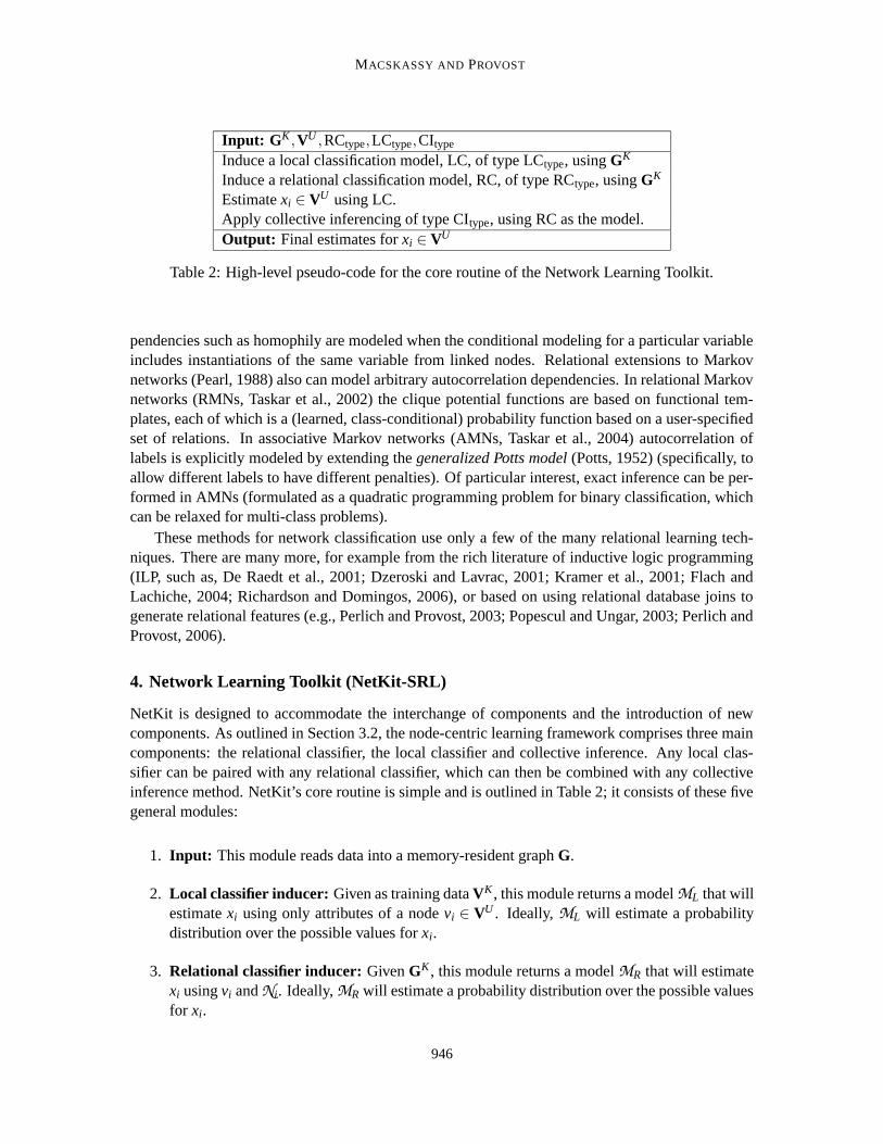
Table 2: High-level pseudo-code for the core routine of the Network Learning Toolkit.
pendencies such as homophily are modeled when the conditional modeling for a particular variableincludes instantiations of the same variable from linked nodes. Relational extensions to Markovnetworks (Pearl, 1988) also can model arbitrary autocorrelation dependencies. In relational Markovnetworks (RMNs, Taskar et al., 2002) the clique potential functions are based on functional tem-plates, each of which is a (learned, class-conditional) probability function based on a user-specifiedset of relations. In associative Markov networks (AMNs, Taskar et al., 2004) autocorrelation oflabels is explicitly modeled by extending the generalized Potts model (Potts, 1952) (specifically, toallow different labels to have different penalties). Of particular interest, exact inference can be per-formed in AMNs (formulated as a quadratic programming problem for binary classification, whichcan be relaxed for multi-class problems).
These methods for network classification use only a few of the many relational learning tech-niques. There are many more, for example from the rich literature of inductive logic programming(ILP, such as, De Raedt et al., 2001; Dzeroski and Lavrac, 2001; Kramer et al., 2001; Flach andLachiche, 2004; Richardson and Domingos, 2006), or based on using relational database joins togenerate relational features (e.g., Perlich and Provost, 2003; Popescul and Ungar, 2003; Perlich andProvost, 2006).
4. Network Learning Toolkit (NetKit-SRL)
NetKit is designed to accommodate the interchange of components and the introduction of newcomponents. As outlined in Section 3.2, the node-centric learning framework comprises three maincomponents: the relational classifier, the local classifier and collective inference. Any local clas-sifier can be paired with any relational classifier, which can then be combined with any collectiveinference method. NetKit’s core routine is simple and is outlined in Table 2; it consists of these fivegeneral modules:
1. Input: This module reads data into a memory-resident graph G.
2. Local classifier inducer: Given as training data VK , this module returns a model ML that willestimate xi using only attributes of a node vi ∈ VU . Ideally, ML will estimate a probabilitydistribution over the possible values for xi.
3. Relational classifier inducer: Given GK , this module returns a model MR that will estimatexi using vi and Ni. Ideally, MR will estimate a probability distribution over the possible valuesfor xi.
946

CLASSIFICATION IN NETWORKED DATA
4. Collective Inferencing: Given a graph G possibly with some xi known, a set of prior esti-mates for xU , and a relational model MR, this module applies collective inferencing to esti-mate xU .
5. Weka Wrapper: This module is a wrapper for Weka5 (Witten and Frank, 2000) and canconvert the graph representation of vi into an entity that can either be learned from or be usedto estimate xi. NetKit can use a Weka classifier either as a local classifier or as a relationalclassifier (by using various aggregation methods to summarize the values of attributes in Ni).
The current version of NetKit-SRL, while able to read in heterogeneous graphs, only supportsclassification in graphs consisting of a single type of node. Algorithms based on expectation max-imization are possible to implement through the NetKit collective inference module, by having thecollective inference module repeatedly apply a relational classifier to learn a new relational modeland then apply the new relational model to G (rather than repeatedly apply the same learned modelat every iteration).
The rest of this section describes the particular relational classifiers and collective inferencemethods implemented in NetKit for the case study. First, we describe the four (univariate6) rela-tional classifiers. Then, we describe the three collective inference methods.
4.1 Relational Classifiers
All four relational classifiers take advantage of the first-order Markov assumption on the network:only a node’s local neighborhood is necessary for classification. The univariate case renders thisassumption particularly restrictive: only the class labels of the local neighbors are necessary. Thelocal network is defined by the user, analogous to the user’s definition of the feature set for proposi-tional learning. Entities whose class labels are not known are either ignored or are assigned a priorprobability, depending upon the choice of local classifier.
4.1.1 WEIGHTED-VOTE RELATIONAL NEIGHBOR CLASSIFIER (WVRN)
The case study’s simplest classifier (Macskassy and Provost, 2003)7 estimates class-membershipprobabilities by assuming the existence of homophily (see Section 3.4).
Definition. Given vi ∈ VU , the weighted-vote relational-neighbor classifier (wvRN) estimatesP(xi|Ni) as the (weighted) mean of the class-membership probabilities of the entities in Ni:
P(xi = c|Ni) =1Z ∑
v j∈Ni
wi, j ·P(x j = c|N j),
where Z is the usual normalizer. This can be viewed simply as an inference procedure, or as aprobability model. In the latter case, it corresponds exactly to the Gaussian-field model discussedbelow in Section 3.5.2. How to conduct the inference/estimate the model falls on the collectiveinference procedure.
5. We use version 3.4.2. Weka is available at http://www.cs.waikato.ac.nz/˜ml/weka/.6. The open-source NetKit release contains multivariate versions of these classifiers.7. Previously called the probabilistic Relational Neighbor classifier (pRN).
947

MACSKASSY AND PROVOST
4.1.2 CLASS-DISTRIBUTION RELATIONAL NEIGHBOR CLASSIFIER (CDRN)
The simple wvRN assumes that neighboring class labels were likely to be the same. Learning amodel of the distribution of neighbor class labels is more flexible, and may lead to better discrimi-nation. Following Perlich and Provost (2003, 2006), and in the spirit of Rocchio’s method (Rocchio,1971), we define node vi’s class vector CV(vi) to be the vector of summed linkage weights to thevarious (known) classes, and class c’s reference vector RV(c) to be the average of the class vectorsfor nodes known to be of class c. Specifically:
CV(vi)k = ∑v j∈Ni,x j=ck
wi, j, (1)
where CV(vi)k represents the kth position in the class vector and ck ∈ X is the kth class. Based onthese class vectors, the reference vectors can then be defined as the normalized vector sum:
RV(c) =1|VK
c |∑
vi∈VKc
CV(vi), (2)
where VKc = {vi|vi ∈ VK ,xi = c}.
For the case study, during training, neighbors in VU are ignored. For prediction, estimated classmembership probabilities are used for neighbors in VU , and Equation 1 becomes:
CV(vi)k = ∑v j∈Ni
wi, j ·P(x j = ck|N j). (3)
Definition. Given vi ∈ VU , the class-distribution relational-neighbor classifier (cdRN) esti-mates the probability of class membership, P(xi = c|Ni), by the normalized vector similarity be-tween vi’s class vector and class c’s reference vector:
P(xi = c|Ni) = sim(CV(vi),RV(c)),
where sim(a,b) is any vector similarity function (L1, L2, cosine, etc.), normalized to lie in the range[0,1]. For the results presented below, we use cosine similarity.
As with wvRN, Equation 3 is a recursive definition, and therefore the value of P(x j = c|N j) isapproximated by the “current” estimate as defined by the selected collective inference technique.
4.1.3 NETWORK-ONLY BAYES CLASSIFIER (NBC)
NetKit’s network-only Bayes classifier (nBC) is based on the algorithm described by Chakrabartiet al. (1998). To start, assume there is a single node vi in VU . The nBC uses multinomial naiveBayesian classification based on the classes of vi’s neighbors.
P(xi = c|Ni) =P(Ni|c) ·P(c)
P(Ni),
where
P(Ni|c) =1Z ∏
v j∈Ni
P(x j = x j|xi = c)wi, j
948

CLASSIFICATION IN NETWORKED DATA
where Z is a normalizing constant and x j is the class observed at node v j. As usual, because P(Ni)is the same for all classes, normalization across the classes allows us to avoid explicitly computingit.
We call nBC “network-only” to emphasize that in the application to the univariate case studybelow, we do not use local attributes of a node. As discussed above, Chakrabarti et al. initializenodes’ priors based on a naive Bayes model over the local document text and add a text-basedterm to the node probability formula.8 In the univariate setting, local text is not available. Wetherefore use the same scheme as for the other relational classifiers: initialize unknown labels asdecided by the local classifier being used (in our study: either the class prior or ’null’, dependingon the collective inference component, as described below). If a neighbor’s label is ’null’, then itis ignored for classification. Also, Chakrabarti et al. differentiated between incoming and outgoinglinks, whereas we do not. Finally, Chakrabarti et al. do not mention how or whether they accountfor possible zeros in the estimations of the marginal conditional probabilities; we apply traditionalLaplace smoothing where m = |X |, the number of classes.
The foregoing assumes all neighbor labels are known. When the values of some neighborsare unknown, but estimations are available, we follow Chakrabarti et al. (1998) and perform aBayesian combination based on (estimated) configuration priors and the entity’s known neighbors.Chakrabarti et al. (1998) describe this procedure in detail. For our case study, such an estimation isnecessary only when using relaxation labeling (described below).
4.1.4 NETWORK-ONLY LINK-BASED CLASSIFICATION (NLB)
The final relational classifier used in the case study is a network-only derivative of the link-basedclassifier (Lu and Getoor, 2003). The network-only Link-Based classifier (nLB) creates a featurevector for a node by aggregating the labels of neighboring nodes, and then uses logistic regressionto build a discriminative model based on these feature vectors. This learned model is then appliedto estimate P(xi = c|Ni). As with the nBC, the difference between the “network-only” link-basedclassifier and Lu and Getoor’s version is that for the univariate case study we do not consider localattributes (e.g., text).
As described above, Lu and Getoor (2003) considered various aggregation methods: existence(binary), the mode, and value counts. The last aggregation method, the count model, is equivalentto the class vector CV(vi) defined in Equation 3. This was the best performing method in the studyby Lu and Getoor, and is the method on which we base nLB. The logistic regression classifier usedby nLB is the multiclass implementation from Weka version 3.4.2.
We made one minor modification to the original link-based classifier. Perlich (2003) argues thatin different situations it may be preferable to use either vectors based on raw counts (as given above)or vectors based on normalized counts. We did preliminary runs using both. The normalized vectorsgenerally performed better, and so we use them for the case study.
4.2 Collective Inference Methods
This section describes three collective inferencing methods implemented in NetKit and used inthe case study. As described above, given (i) a network initialized by the local model, and (ii)a relational model, a collective inference method infers a set of class labels for xU . Depending
8. The original classifier was defined as: P(xi = c|Ni) = P(Ni|c) ·P(τi|vi) ·P(c), with τi being the text of the document-entity represented by vertex vi.
949
MACSKASSY AND PROVOST
1. Initialize vi ∈ VU using the local classifier model, ML. Specifically, for vi ∈ VU :
(a) ci←ML(vi), where ci is a vector of probabilities representing ML’s estimatesof P(xi|Ni). We use ci(k) to mean the kth value in ci, which representsP(xi = ck|Ni).
For the case study, the local classifier model returns the unconditionalmarginal class distribution estimated from xK .
(b) Sample a value cs from ci, such that P(cs = ck|ci) = ci(k).
(c) Set xi← cs.
2. Generate a random ordering, O, of vertices in VU .
3. For elements vi ∈ O in order:
(a) Apply the relational classifier model: ci←MR(vi).
(b) Sample a value cs from ci, such that P(cs = ck|ci) = ci(k).
(c) Set xi← cs.Note that when MR is applied to estimate ci it uses the “new” labelingsfrom elements 1, . . . ,(i−1), while using the “current” labelings for elements(i+1), . . . ,n.
4. Repeat prior step 200 times without keeping any statistics. This is known as theburnin period.
5. Repeat again for 2000 iterations, counting the number of times each Xi is assigneda particular value c ∈ X . Normalizing these counts forms the final class probabilityestimates.
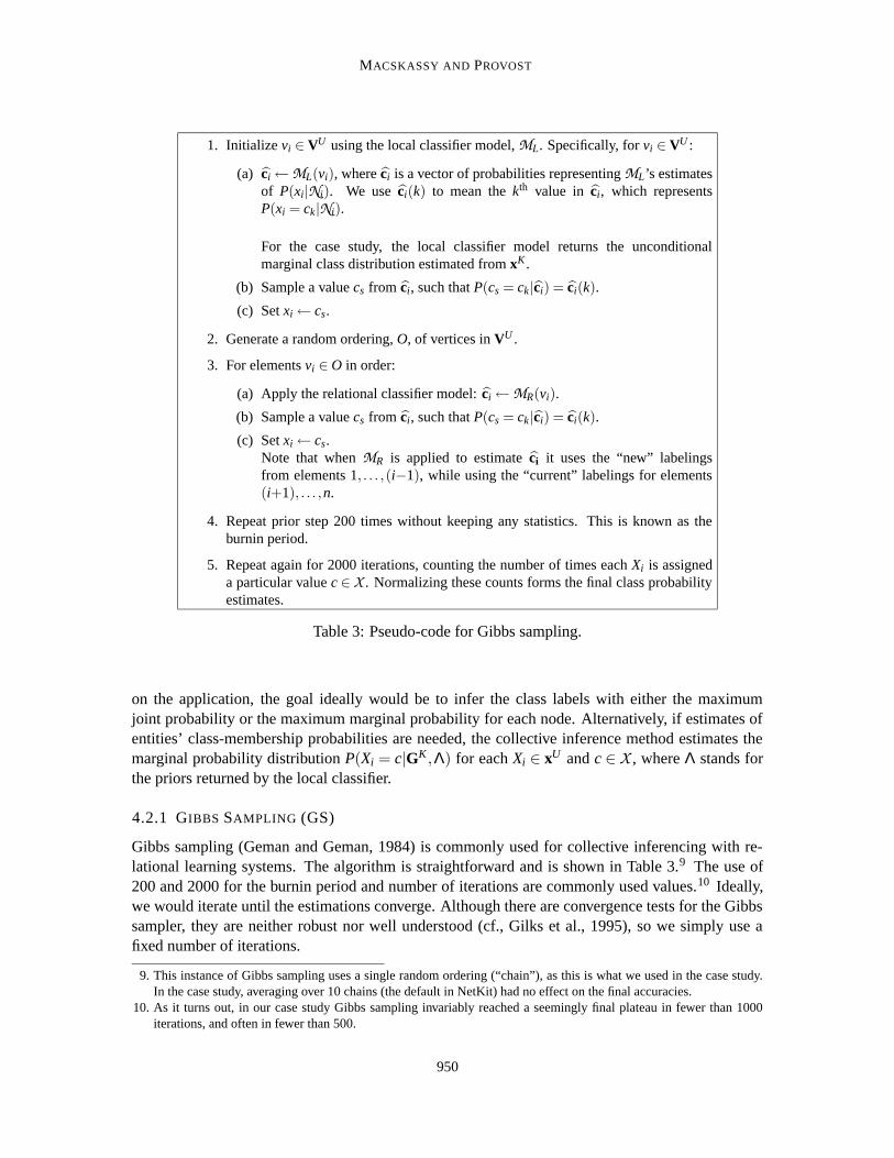
Table 3: Pseudo-code for Gibbs sampling.
on the application, the goal ideally would be to infer the class labels with either the maximumjoint probability or the maximum marginal probability for each node. Alternatively, if estimates ofentities’ class-membership probabilities are needed, the collective inference method estimates themarginal probability distribution P(Xi = c|GK ,Λ) for each Xi ∈ xU and c ∈ X , where Λ stands forthe priors returned by the local classifier.
4.2.1 GIBBS SAMPLING (GS)
Gibbs sampling (Geman and Geman, 1984) is commonly used for collective inferencing with re-lational learning systems. The algorithm is straightforward and is shown in Table 3.9 The use of200 and 2000 for the burnin period and number of iterations are commonly used values.10 Ideally,we would iterate until the estimations converge. Although there are convergence tests for the Gibbssampler, they are neither robust nor well understood (cf., Gilks et al., 1995), so we simply use afixed number of iterations.
9. This instance of Gibbs sampling uses a single random ordering (“chain”), as this is what we used in the case study.In the case study, averaging over 10 chains (the default in NetKit) had no effect on the final accuracies.
10. As it turns out, in our case study Gibbs sampling invariably reached a seemingly final plateau in fewer than 1000iterations, and often in fewer than 500.
950

CLASSIFICATION IN NETWORKED DATA
1. For vi ∈ VU , initialize the prior: ci(0)←ML(vi), where ci is defined as in Table 3.
For the case study, the local classifier model returns the unconditional marginal classdistribution estimated from xK .
2. For elements vi ∈ VU :
(a) Estimate xi by applying the relational model:
ci(t+1)←MR(v(t)
i ), (4)
where MR(v(t)i ) denotes using the estimates c j
(t) for v j ∈ Ni, and t is theiteration count. This has the effect that all predictions are done pseudo-simultaneously based on the state of the graph after iteration t.
3. Repeat for T iterations, where T = 99 for the case study. c(T ) will comprise the finalclass probability estimations.
Table 4: Pseudo-code for relaxation labeling.
Notably, because all nodes are assigned a class at every iteration, when Gibbs sampling is usedthe relational models will always see a fully labeled/classified neighborhood, making predictionstraightforward. For example, nBC does not need to compute its Bayesian combination (see Sec-tion 4.1.3).
4.2.2 RELAXATION LABELING (RL)
The second collective inferencing method used in the study is relaxation labeling, based on themethod of Chakrabarti et al. (1998). Rather than treat G as being in a specific labeling “state” atevery point (as Gibbs sampling does), relaxation labeling retains the uncertainty, keeping track of thecurrent probability estimations for xU . The relational model must be able to use these estimations.Further, rather than estimating one node at a time and updating the graph right away, relaxationlabeling “freezes” the current estimations so that at step t + 1 all vertices will be updated based onthe estimations from step t. The algorithm is shown in Table 4.
Preliminary runs showed that relaxation labeling sometimes does not converge, but rather endsup oscillating between two or more graph states.11 NetKit performs simulated annealing—on eachsubsequent iteration giving more weight to a node’s own current estimate and less to the influenceof its neighbors.
The new updating step, replacing Equation 4 is:
ci(t+1) = β(t+1) ·MR(v(t)
i )+(1−β(t+1)) · ci(t),
where
β0 = k,
β(t+1) = β(t) ·α,
11. Such oscillation has been noted elsewhere for closely related methods (Murphy et al., 1999).
951
MACSKASSY AND PROVOST
1. For vi ∈ VU , initialize the prior: ci←ML(vi), where ci is defined as in Table 3. Thelink-based classification work of Lu and Getoor (2003) uses a local classifier to setinitial classifications. This will clearly not work in our case (all unknowns would beclassified as the majority class), and we therefore use a local classifier model whichreturns null (i.e., it does not return an estimation.)
2. Generate a random ordering, O, of elements in VU .
3. For elements vi ∈ O:
(a) Apply the relational classifier model, ci←MR, using all non-null labels (en-tities which have not yet been classified will be ignored.) If all neighbor enti-ties are null, then return null.
(b) Classify vi:
xi = ck,k = argmax j ci( j),
where ci( j) is the jth value in vector ci. (Remember, ci is a vector of |X |elements. We classify vi by predicting the class with the highest likelihood).
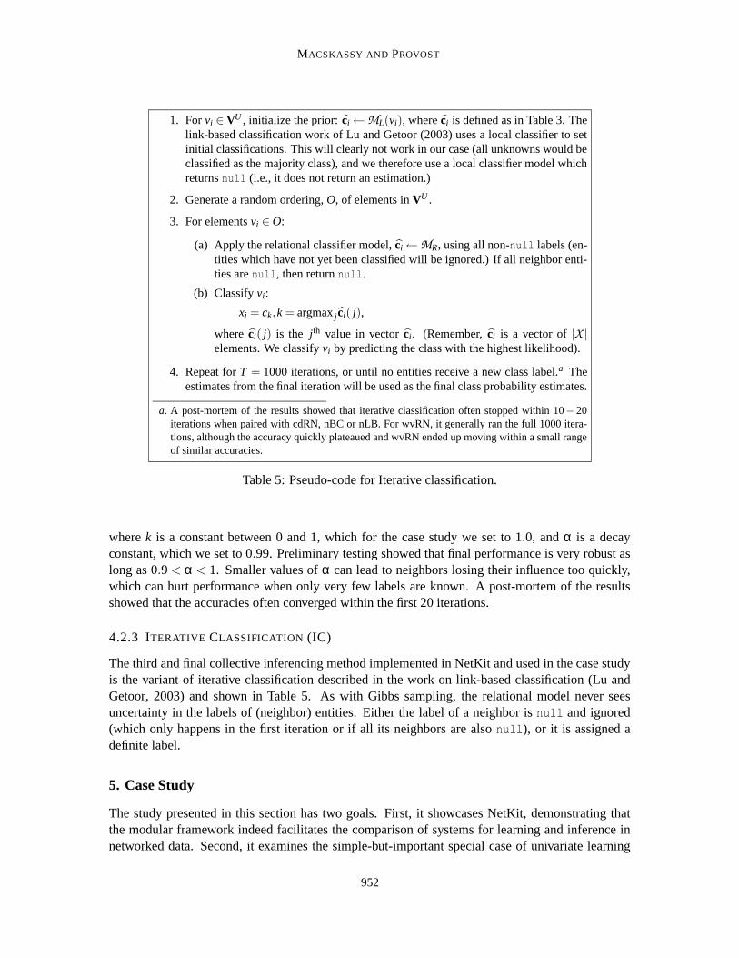
4. Repeat for T = 1000 iterations, or until no entities receive a new class label.a Theestimates from the final iteration will be used as the final class probability estimates.
a. A post-mortem of the results showed that iterative classification often stopped within 10− 20iterations when paired with cdRN, nBC or nLB. For wvRN, it generally ran the full 1000 itera-tions, although the accuracy quickly plateaued and wvRN ended up moving within a small rangeof similar accuracies.
Table 5: Pseudo-code for Iterative classification.
where k is a constant between 0 and 1, which for the case study we set to 1.0, and α is a decayconstant, which we set to 0.99. Preliminary testing showed that final performance is very robust aslong as 0.9 < α < 1. Smaller values of α can lead to neighbors losing their influence too quickly,which can hurt performance when only very few labels are known. A post-mortem of the resultsshowed that the accuracies often converged within the first 20 iterations.
4.2.3 ITERATIVE CLASSIFICATION (IC)
The third and final collective inferencing method implemented in NetKit and used in the case studyis the variant of iterative classification described in the work on link-based classification (Lu andGetoor, 2003) and shown in Table 5. As with Gibbs sampling, the relational model never seesuncertainty in the labels of (neighbor) entities. Either the label of a neighbor is null and ignored(which only happens in the first iteration or if all its neighbors are also null), or it is assigned adefinite label.
5. Case Study
The study presented in this section has two goals. First, it showcases NetKit, demonstrating thatthe modular framework indeed facilitates the comparison of systems for learning and inference innetworked data. Second, it examines the simple-but-important special case of univariate learning
952

CLASSIFICATION IN NETWORKED DATA
and inference in homogeneous networks, comparing alternative techniques that have not before beencompared systematically, if at all. The setting for the case study is simple: For some entities in thenetwork, the value of xi is known; for others it must be estimated.
Univariate classification, albeit a simplification for many domains, is important for several rea-sons. First, it is a representation that is used in some applications. Above we mentioned fraud detec-tion; as a specific example, a telephone account that calls the same numbers as a known fraudulentaccount (and hence the accounts are connected through these intermediary numbers) is suspicious(Fawcett and Provost, 1997; Cortes et al., 2001). For phone fraud, univariate network classificationoften provides alarms with reasonable coverage and remarkably low false-positive rates. Gener-ally speaking, a homogeneous, univariate network is an inexpensive (in terms of data gathering,processing, storage) approximation of many complex networked data problems. Fraud detectionapplications certainly do have a variety of additional attributes of importance; nevertheless, univari-ate simplifications are very useful and are used in practice.
The univariate case also is important scientifically. It isolates a primary difference betweennetworked data and non-networked data, facilitating the analysis and comparison of relevant clas-sification and learning methods. One thesis of this study is that there is considerable informationinherent in the structure of the networked data and that this information can be readily taken advan-tage of, using simple models, to estimate the labels of unknown entities. This thesis is tested byisolating this characteristic—namely ignoring any auxiliary attributes and only allowing the use ofknown class labels—and empirically evaluating how well univariate models perform in this settingon benchmark data sets.
Considering homogeneous networks plays a similar role. Although the domains we considerhave obvious representations consisting of multiple entity types and edges (e.g., people and papersfor node types and same-author-as and cited-by as edge types in a citation-graph domain), a homo-geneous representation is much simpler. In order to assess whether a more complex representationis worthwhile, it is necessary to assess standard techniques on the simpler representation (as we doin this case study). Of course, the way a network is “homogenized” may have a considerable effecton classification performance. We will revisit this below in Section 5.3.6.
5.1 Data
The case study reported in this paper makes use of 12 benchmark data sets from four domains thathave been the subject of prior study in machine learning. As this study focuses on networked data,any singleton (disconnected) entities in the data were removed. Therefore, the statistics we presentmay differ from those reported previously.
5.1.1 IMDB
Networked data from the Internet Movie Database (IMDb)12 have been used to build models pre-dicting movie success as determined by box-office receipts (Jensen and Neville, 2002a). Followingthe work of Neville et al. (2003), we focus on movies released in the United States between 1996and 2001 with the goal of estimating whether the opening weekend box-office receipts “will” ex-ceed $2 million (Neville et al., 2003). Obtaining data from the IMDb web-site, we identified 1169movies released between 1996 and 2001 that we were able to link up with a revenue classification
12. See http://www.imdb.com.
953

MACSKASSY AND PROVOST
Category SizeHigh-revenue 572Low-revenue 597Total 1169Base accuracy 51.07%
Table 6: Class distribution for the IMDb data set.
Category SizeCase-based 402Genetic Algorithms 551Neural Networks 1064Probabilistic Methods 529Reinforcement Learning 335Rule Learning 230Theory 472Total 3583Base accuracy 29.70%
Table 7: Class distribution for the cora data set.
in the database given to us by the authors of the original study. The class distribution of the data setis shown in Table 6.
We link movies if they share a production company, based on observations from previous work(Macskassy and Provost, 2003).13 The weight of an edge in the resulting graph is the number ofproduction companies two movies have in common. Notably, we ignore the temporal aspect of themovies in this study, simply labeling movies at random for the training set. This can result in amovie in the test set being released earlier than a movie in the training set.
5.1.2 CORA
The cora data set (McCallum et al., 2000) comprises computer science research papers. It includesthe full citation graph as well as labels for the topic of each paper (and potentially sub- and sub-sub-topics).14 Following a prior study (Taskar et al., 2001), we focused on papers within the machinelearning topic with the classification task of predicting a paper’s sub-topic (of which there are seven).The class distribution of the data set is shown in Table 7.
Papers can be linked if they share a common author, or if one cites the other. Following priorwork (Lu and Getoor, 2003), we link two papers if one cites the other. The weight of an edge wouldnormally be one unless the two papers cite each other (in which case it is two—there can be no otherweight for existing edges).
13. And on a suggestion from David Jensen.14. These labels were assigned by a naive Bayes classifier (McCallum et al., 2000).
954
CLASSIFICATION IN NETWORKED DATA
Number of web-pagesClass Cornell Texas Washington Wisconsinstudent 145 163 151 155not-student 201 171 283 193Total 346 334 434 348Base accuracy 58.1% 51.2% 60.8% 55.5%
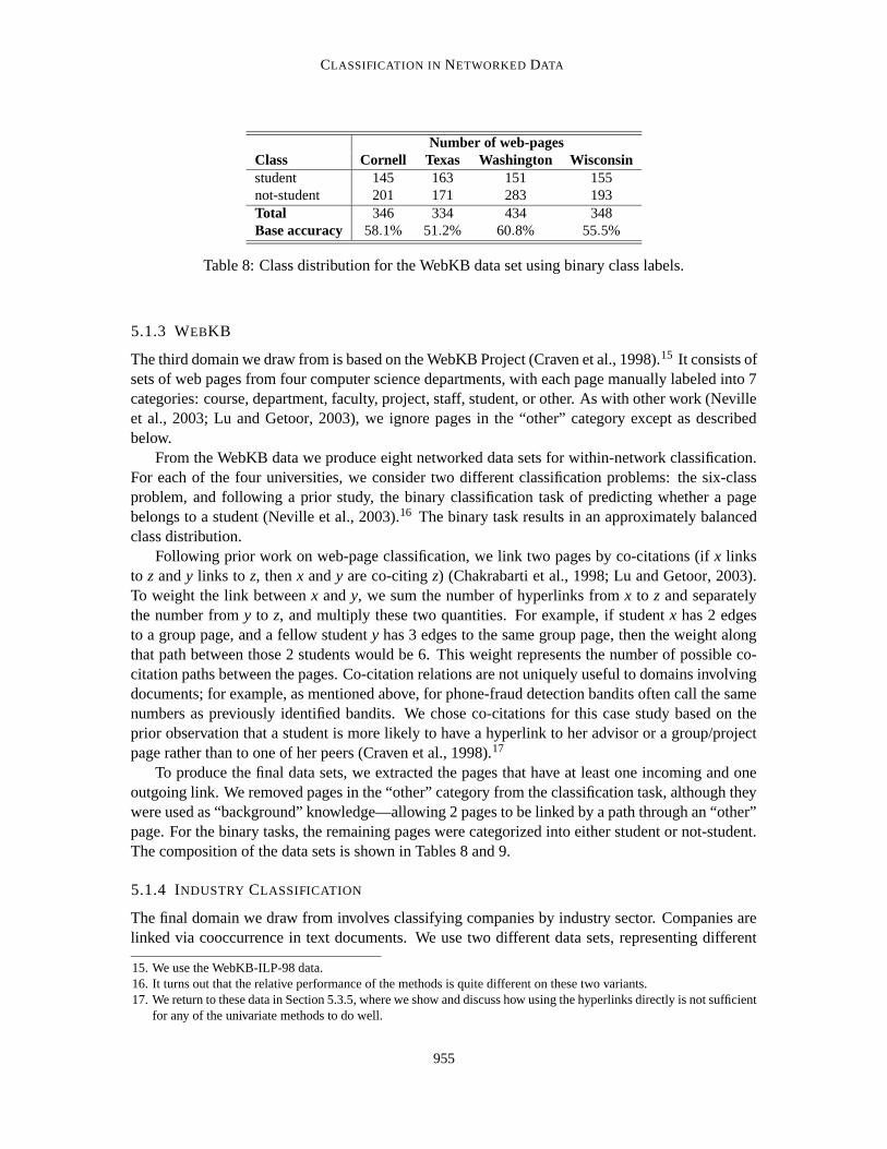
Table 8: Class distribution for the WebKB data set using binary class labels.
5.1.3 WEBKB
The third domain we draw from is based on the WebKB Project (Craven et al., 1998).15 It consists ofsets of web pages from four computer science departments, with each page manually labeled into 7categories: course, department, faculty, project, staff, student, or other. As with other work (Nevilleet al., 2003; Lu and Getoor, 2003), we ignore pages in the “other” category except as describedbelow.
From the WebKB data we produce eight networked data sets for within-network classification.For each of the four universities, we consider two different classification problems: the six-classproblem, and following a prior study, the binary classification task of predicting whether a pagebelongs to a student (Neville et al., 2003).16 The binary task results in an approximately balancedclass distribution.
Following prior work on web-page classification, we link two pages by co-citations (if x linksto z and y links to z, then x and y are co-citing z) (Chakrabarti et al., 1998; Lu and Getoor, 2003).To weight the link between x and y, we sum the number of hyperlinks from x to z and separatelythe number from y to z, and multiply these two quantities. For example, if student x has 2 edgesto a group page, and a fellow student y has 3 edges to the same group page, then the weight alongthat path between those 2 students would be 6. This weight represents the number of possible co-citation paths between the pages. Co-citation relations are not uniquely useful to domains involvingdocuments; for example, as mentioned above, for phone-fraud detection bandits often call the samenumbers as previously identified bandits. We chose co-citations for this case study based on theprior observation that a student is more likely to have a hyperlink to her advisor or a group/projectpage rather than to one of her peers (Craven et al., 1998).17
To produce the final data sets, we extracted the pages that have at least one incoming and oneoutgoing link. We removed pages in the “other” category from the classification task, although theywere used as “background” knowledge—allowing 2 pages to be linked by a path through an “other”page. For the binary tasks, the remaining pages were categorized into either student or not-student.The composition of the data sets is shown in Tables 8 and 9.
5.1.4 INDUSTRY CLASSIFICATION
The final domain we draw from involves classifying companies by industry sector. Companies arelinked via cooccurrence in text documents. We use two different data sets, representing different
15. We use the WebKB-ILP-98 data.16. It turns out that the relative performance of the methods is quite different on these two variants.17. We return to these data in Section 5.3.5, where we show and discuss how using the hyperlinks directly is not sufficient
for any of the univariate methods to do well.
955
MACSKASSY AND PROVOST
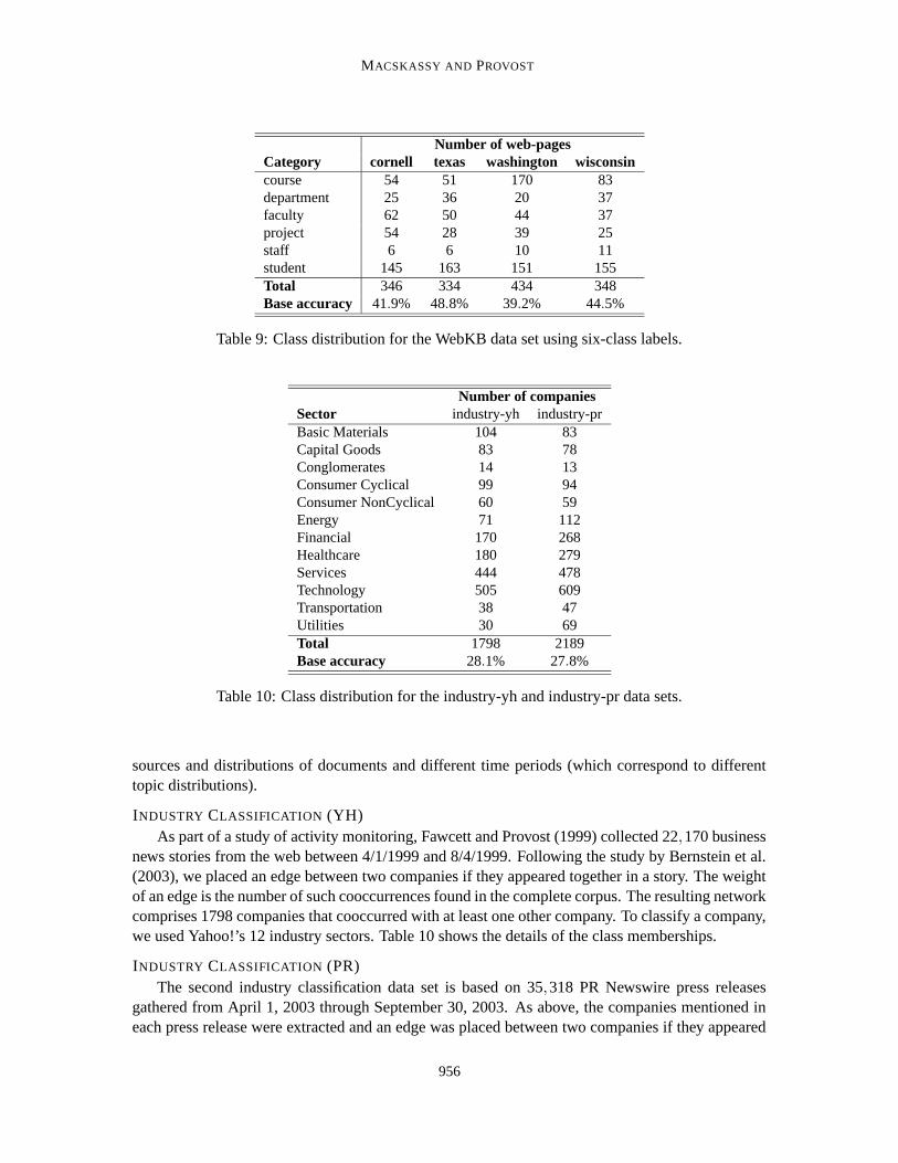
Number of web-pagesCategory cornell texas washington wisconsincourse 54 51 170 83department 25 36 20 37faculty 62 50 44 37project 54 28 39 25staff 6 6 10 11student 145 163 151 155Total 346 334 434 348Base accuracy 41.9% 48.8% 39.2% 44.5%
Table 9: Class distribution for the WebKB data set using six-class labels.
Number of companiesSector industry-yh industry-prBasic Materials 104 83Capital Goods 83 78Conglomerates 14 13Consumer Cyclical 99 94Consumer NonCyclical 60 59Energy 71 112Financial 170 268Healthcare 180 279Services 444 478Technology 505 609Transportation 38 47Utilities 30 69Total 1798 2189Base accuracy 28.1% 27.8%
Table 10: Class distribution for the industry-yh and industry-pr data sets.
sources and distributions of documents and different time periods (which correspond to differenttopic distributions).
INDUSTRY CLASSIFICATION (YH)As part of a study of activity monitoring, Fawcett and Provost (1999) collected 22,170 business
news stories from the web between 4/1/1999 and 8/4/1999. Following the study by Bernstein et al.(2003), we placed an edge between two companies if they appeared together in a story. The weightof an edge is the number of such cooccurrences found in the complete corpus. The resulting networkcomprises 1798 companies that cooccurred with at least one other company. To classify a company,we used Yahoo!’s 12 industry sectors. Table 10 shows the details of the class memberships.
INDUSTRY CLASSIFICATION (PR)The second industry classification data set is based on 35,318 PR Newswire press releases
gathered from April 1, 2003 through September 30, 2003. As above, the companies mentioned ineach press release were extracted and an edge was placed between two companies if they appeared
956

CLASSIFICATION IN NETWORKED DATA
together in a press release. The weight of an edge is the number of such cooccurrences found in thecomplete corpus. The resulting network comprises 2189 companies that cooccurred with at leastone other company. To classify a company, we use the same classification scheme from Yahoo! asbefore. Table 10 shows the details of the class memberships.
5.2 Experimental Methodology
NetKit allows for any combination of a local classifier (LC), a relational classifier (RC) and acollective inferencing method (CI). If we consider an LC-RC-CI configuration to be a completenetwork-classification method, we have 12 to compare on each data set. Since, for this paper, thelocal classifier component is directly tied to the collective inference component (our local classifiercomponents determine priors based on which collective inference component is being used), wehenceforth consider a network-classification method to be an RC-CI configuration.
We first verify that the network structure alone (linkages plus known class labels) often con-tains a considerable amount of useful information for entity classification. We vary from 10% to90% the percentage of nodes in the network for which class membership is known initially.18 Thestudy assesses: (1) whether the network structure enables accurate classification; (2) how muchprior information is needed in order to perform well, and (3) whether there are regular patterns ofimprovement across methods as the percentage of initially known labels increases.
Accuracy is averaged over 10 runs. Specifically, given a data set, G = (V,E), the subset ofentities with known labels VK (the “training” data set19) is created by selecting a class-stratifiedrandom sample of (100× r)% of the entities in V. The test set, VU , is then defined as V−VK .We prune VU by removing all nodes in zero-knowledge components—nodes for which there is nopath to any node in VK . We use the same 10 training/test partitions for each network-classificationmethod. Although it would be desirable to keep the test data disjoint (and therefore independent)as done in traditional machine learning via methods such as cross-validation, this is not applicablefor within-network learning. We keep the test node sets disjoint as much as possible between thedifferent runs. For example, at r = 0.90 (90% labeled data), our sets of training and testing nodesfollow standard class-stratified 10-fold cross-validation.
5.3 Results
This section describes the results for our case study as well as follow-up experiments that clar-ify some of our findings. We start by verifying that there is information in the network structurealone (Section 5.3.1), then study the collective inference (Section 5.3.2) and relational classifier(Section 5.3.3) components separately, and then compare the network-classification methods (Sec-tion 5.3.4). We then revisit how edges were selected—we study the effects of badly chosen edges(Section 5.3.5) and then provide one method for automatic selection of edges (Section 5.3.6). Weend in Section 5.3.7 with a discussion of the use of network-only methods as a baseline method thatis as important as the standard non-relational-classifier baseline comparison.
957

MACSKASSY AND PROVOST
0
0.2
0.4
0.6
0.8
1
0 0.2 0.4 0.6 0.8 1
Acc
urac
y
Ratio Labeled
cora_cite
0
0.2
0.4
0.6
0.8
1
0 0.2 0.4 0.6 0.8 1
Acc
urac
y
Ratio Labeled
cornellB_cocite
0
0.2
0.4
0.6
0.8
1
0 0.2 0.4 0.6 0.8 1
Acc
urac
y
Ratio Labeled
cornellM_cocite
0
0.2
0.4
0.6
0.8
1
0 0.2 0.4 0.6 0.8 1
Acc
urac
y
Ratio Labeled
imdb_prodco
0
0.2
0.4
0.6
0.8
1
0 0.2 0.4 0.6 0.8 1
Acc
urac
y
Ratio Labeled
texasB_cocite
0
0.2
0.4
0.6
0.8
1
0 0.2 0.4 0.6 0.8 1
Acc
urac
y
Ratio Labeled
texasM_cocite
0
0.2
0.4
0.6
0.8
1
0 0.2 0.4 0.6 0.8 1
Acc
urac
y
Ratio Labeled
industry-pr
0
0.2
0.4
0.6
0.8
1
0 0.2 0.4 0.6 0.8 1
Acc
urac
y
Ratio Labeled
washingtonB_cocite
0
0.2
0.4
0.6
0.8
1
0 0.2 0.4 0.6 0.8 1
Acc
urac
y
Ratio Labeled
washingtonM_cocite
0
0.2
0.4
0.6
0.8
1
0 0.2 0.4 0.6 0.8 1
Acc
urac
y
Ratio Labeled
industry-yh
0
0.2
0.4
0.6
0.8
1
0 0.2 0.4 0.6 0.8 1
Acc
urac
y
Ratio Labeled
wisconsinB_cocite
0
0.2
0.4
0.6
0.8
1
0 0.2 0.4 0.6 0.8 1
Acc
urac
y
Ratio Labeled
wisconsinM_cocite
Figure 1: Overall classification accuracies on the twelve data sets. Horizontal lines represent pre-dicting the most prevalent class. These graphs are shown to display trends and not todistinguish the twelve methods; individual methods will be clarified in subsequent dis-cussion. The horizontal axis plots the fraction (r) of a network’s nodes for which theclass label is known. In each case, when many labels are known (right end) there is aset of methods that performs well. When few labels are known (left end) there is muchmore variation in performance. Data sets are tagged based on the edge-type used, where‘prodco’ on the IMDb data is short for ‘production company’, and ‘B’ and ‘M’ in theWebKB data sets represent ‘binary’ and ‘multi-class’ respectively.
958

CLASSIFICATION IN NETWORKED DATA
0
0.2
0.4
0.6
0.8
1
0 0.2 0.4 0.6 0.8 1
Acc
urac
y
Ratio Labeled
cora_cite - wvRN
RLICGS
base accuracy 0
0.2
0.4
0.6
0.8
1
0 0.2 0.4 0.6 0.8 1
Acc
urac
y
Ratio Labeled
imdb_prodco - wvRN
RLICGS
base accuracy 0
0.2
0.4
0.6
0.8
1
0 0.2 0.4 0.6 0.8 1
Acc
urac
y
Ratio Labeled
wisconsinB_cocite - wvRN
RLICGS
base accuracy
0
0.2
0.4
0.6
0.8
1
0 0.2 0.4 0.6 0.8 1
Acc
urac
y
Ratio Labeled
cora_cite - cdRN
RLICGS
base accuracy 0
0.2
0.4
0.6
0.8
1
0 0.2 0.4 0.6 0.8 1
Acc
urac
y
Ratio Labeled
imdb_prodco - cdRN
RLICGS
base accuracy 0
0.2
0.4
0.6
0.8
1
0 0.2 0.4 0.6 0.8 1A
ccur
acy
Ratio Labeled
wisconsinB_cocite - cdRN
RLICGS
base accuracy
0
0.2
0.4
0.6
0.8
1
0 0.2 0.4 0.6 0.8 1
Acc
urac
y
Ratio Labeled
cora_cite - nBC
RLICGS
base accuracy 0
0.2
0.4
0.6
0.8
1
0 0.2 0.4 0.6 0.8 1
Acc
urac
y
Ratio Labeled
imdb_prodco - nBC
RLICGS
base accuracy 0
0.2
0.4
0.6
0.8
1
0 0.2 0.4 0.6 0.8 1
Acc
urac
y
Ratio Labeled
wisconsinB_cocite - nBC
RLICGS
base accuracy
0
0.2
0.4
0.6
0.8
1
0 0.2 0.4 0.6 0.8 1
Acc
urac
y
Ratio Labeled
cora_cite - nLB
RLICGS
base accuracy 0
0.2
0.4
0.6
0.8
1
0 0.2 0.4 0.6 0.8 1
Acc
urac
y
Ratio Labeled
imdb_prodco - nLB
RLICGS
base accuracy 0
0.2
0.4
0.6
0.8
1
0 0.2 0.4 0.6 0.8 1
Acc
urac
y
Ratio Labeled
wisconsinB_cocite - nLB
RLICGS
base accuracy
Figure 2: Comparison of collective inference methods on a few data sets. The three collectiveinference methods are relaxation labeling (RL), iterative classification (IC), and Gibbssampling (GS). The data set and the relational classifier component are listed above eachgraph. The horizontal line represents predicting the most prevalent class.
959

MACSKASSY AND PROVOST
5.3.1 INFORMATION IN THE NETWORK STRUCTURE
Figure 1 shows the accuracies of the 12 network-classification methods across the 12 data sets asthe fraction (r) of entities for which class memberships are known increases from r = 0.1 to r = 0.9.The purpose of these graphs is not to differentiate the curves, but to compare the general trends andthe levels of the accuracies to the baseline accuracies. In the univariate case, if the linkage structureis not known, the only non-subjective alternative is to estimate using the class base rate (prior),which is shown by the horizontal line in the graphs. As is clear from Figure 1, all of the data setscontain considerable information in the class-linkage structure. The worst relative performance ison industry-pr, where at the right end of the curves the error rate nonetheless is reduced by 30–40%.The best performance is on the binary-class WebKB-texas, where the best methods reduce the errorrate by close to 90%. And in most cases, the better methods reduce the error rate by over 50%toward the right end of the curves.
Machine learning studies on networked data sets seldom have compared to simple network-classification methods like these, opting instead for comparing to non-relational classification. Theseresults argue strongly that comparisons also should be made to univariate network classification, ifthe purpose is to demonstrate the power of a more sophisticated relational learning method. Wereturn to this argument in Section 5.3.7.
5.3.2 COLLECTIVE INFERENCE COMPONENT
Figure 2 shows, for three of the data sets, the comparative performances of the three collectiveinference components. Each graph is for a particular relational classifier. The graphs show thatwhile the three components often perform similarly, their performances are clearly separated forlow values of r.
Table 11 shows the p-values for a Wilcoxon signed-rank test assessing whether the first methodlisted in column 1 is significantly better than the second. Specifically, for a given data set and labelratio (r), each network-classification experiment consists of 10 random train/test splits—the samefor all configurations. For each pair of collective inference components, averaging the accuracies ofthe 10 splits across the 4 relational classifier components gives one average accuracy score for eachof the 12 data sets yielding 12 paired data points for each collective inference method. The resultsshow clearly that relaxation labeling, across the board, outperforms Gibbs sampling at p≤ 0.01 andthat relaxation labeling is also better than iterative classification across the board. Further, we seethat iterative classification and Gibbs sampling are roughly comparable.
The foregoing gives some evidence that relaxation labeling is consistently better than iterativeclassification and Gibbs sampling when the results are pooled, especially at low values of r. Table 12quantifies the differences. In order to be comparable across data sets with different base rates, thetable shows the amount of error reduction over the base rate. As a simple example, assume the baseerror rate is 0.4, method A yields an error rate of 0.1, and method B yields an error rate of 0.2.Method A reduces the error by 75%. Method B reduces the error by 50%.
18. We also performed boundary experiments using the weighted-vote relational neighbor classifier with relaxation label-ing, where we decreased the number of initially known labels down to 0.1% of the graph. The classification accuracygenerally degrades gracefully to doing no better than random guessing at this extreme.
19. These data will be used not only for training models, but also as existing background knowledge during classification.
960

CLASSIFICATION IN NETWORKED DATA
sample ratio (r)0.10 0.20 0.30 0.40 0.50 0.60 0.70 0.80 0.90
RL v GS 0.002 0.001 0.001 0.001 0.002 0.001 0.001 0.010 0.010RL v IC 0.025 0.100 0.100 0.025 0.002 0.002 0.001 0.005 0.002IC v GS 0.400 0.450 — 0.450 0.400 — 0.250 — 0.400
Table 11: p-values for the Wilcoxon signed-rank test, comparing the accuracies of pairs of threecollective inference methods across all data sets and relational classifier methods. (Thethree collective inference methods are relaxation labeling (RL), iterative classification(IC), and Gibbs sampling (GS)). For each cell, bold text means that the first method wasbetter than the second method and italics means it was worse. The cells with ’—’ meansthere was no significant difference.
sample ratio (r)0.10 0.20 0.30 0.40 0.50 0.60 0.70 0.80 0.90 overall
RL 0.081 0.184 0.262 0.339 0.409 0.446 0.468 0.491 0.509 0.354IC 0.000 0.116 0.235 0.314 0.382 0.423 0.452 0.482 0.503 0.323
GS 0.029 0.126 0.231 0.301 0.385 0.421 0.450 0.474 0.502 0.324
Table 12: Relative error reductions (ERREL) for each collective inference method across all data setsand relational classifier methods. (The three collective inference methods are relaxationlabeling (RL), iterative classification (IC), and Gibbs sampling (GS)). The last column,overall, is the average error reduction for each method across all sample ratios. Boldentries indicate the largest relative error reduction for each sample ratio.
sample ratio (r)0.10 0.20 0.30 0.40 0.50 0.60 0.70 0.80 0.90 total
RL 11 11 10 7 4 5 6 4 6 64GS 1 1 0 1 5 3 4 4 4 23IC 0 0 2 4 3 4 2 4 2 21
Table 13: Number of times each collective inference method was the best across the 12 data sets.The three methods are relaxation labeling (RL), iterative classification (IC), and Gibbssampling (GS).
The relative error reduction of the collective inference (CI) components is defined as follows:
ERABS(RC,CI,D,r) = (base err(D)− err(RC-CI,D,r)),
ERREL(RC,CI,D,r) =ERABS(RC,CI,D,r)
base err(D),
ERREL(RC,CI,r) =1|D| ∑
D∈DERREL(RC,CI,D,r),
ERREL(CI,r) =1|RC| ∑
RC∈RCERREL(RC,CI,r),
961

MACSKASSY AND PROVOST
where err(RC-CI,D,r) is the error for the RC-CI configuration (a relational classifier paired with acollective inference method) on data set D with r% of the graph being labeled.
Table 12 shows the relative error reductions for each collective inference component. Relaxationlabeling outperformed iterative classification across the board, from as low as a 1.3% improvement(r = 0.90) to as high as 59% or better improvement (r ≤ 0.2) when averaged over all the data setsand relational classifier methods. Overall relaxation labeling improved performance over iterativeclassification by about 10% as seen in the last column. Notably, relaxation labeling’s advantage overiterative classification improves monotonically as less is known in the network. Similar numbersand a similar pattern are seen for relaxation labeling versus Gibbs sampling. Iterative classificationand Gibbs sampling are comparable.
For another perspective, Table 13 shows, for each ratio as well as a total across all ratios, thenumber of times each collective inference implementation took part in the best-performing network-classification combination for each of the 12 data sets. Specifically, for each sampling ratio, eachwin for an RC-CI configuration (relational classifier paired with a collective inference method)counted as a win for the collective inference module of the pair (as well as a win for the relationalclassifier module in the next section). For example, in Figure 2, the first column of four graphs showsthe performances of the 12 network-classification combinations on the cora data; at the left end ofthe curves, wvRN-RL is the best performing combination. Table 13 adds further support to theconclusion that relaxation labeling was the overall best component, primarily due to its advantage atlow values of r. We also see again that Gibbs sampling and iterative classification were comparable.
5.3.3 RELATIONAL CLASSIFIER COMPONENT
Comparing relational models, we would expect to see a certain pattern: if even moderate homophilyis present in the data, we would expect wvRN to perform well. Its nonexistent training variance20
should allow it to perform relatively well, even with small numbers of known labels in the net-work. The higher-variance nLB may perform relatively poorly with small numbers of known labels(primarily because of the lack of training data). On the other hand, wvRN is potentially a very-high-bias classifier—it does not learn a relational model at all. The learning-based classifiers maywell perform better with large numbers of known labels if there are patterns beyond homophilyto be learned. As a worst case for wvRN, consider a bipartite graph between two classes. In aleave-one-out cross-validation, wvRN would be wrong on every prediction. The relational learnersshould notice the true pattern immediately. More generally, one should expect a pattern of curvescrossing with increasing numbers of known labels, similar to learning curves crossing (Perlich et al.,2003): lower variance methods (such as wvRN) should be preferable with fewer known labels; moreflexible learning methods should be preferable with more known labels (thus, more training data).
Figure 3 shows for four of the data sets the performances of the four relational classifier im-plementations. The rows of graphs correspond to data sets and the columns to the three differentcollective inference methods. The graphs show several things. As would be expected, accuracyimproves as more of the network is labeled, although in certain cases classification is remarkablyaccurate with very few known labels (e.g., see cora). One method is substantially worse than theothers. Among the remaining methods, performance often differs greatly with few known labels,and tends to converge with many known labels. More subtly, as expected there often is a crossingof curves when about half the nodes are labeled (e.g., see Washington).
20. There still will be variance due to the set of known labels.
962

CLASSIFICATION IN NETWORKED DATA
0
0.2
0.4
0.6
0.8
1
0 0.2 0.4 0.6 0.8 1
Acc
urac
y
Ratio Labeled
cora_cite - RL
wvRNcdRNnBCnLB
base accuracy 0
0.2
0.4
0.6
0.8
1
0 0.2 0.4 0.6 0.8 1A
ccur
acy
Ratio Labeled
cora_cite - GS
wvRNcdRNnBCnLB
base accuracy 0
0.2
0.4
0.6
0.8
1
0 0.2 0.4 0.6 0.8 1
Acc
urac
y
Ratio Labeled
cora_cite - IC
wvRNcdRNnBCnLB
base accuracy
0
0.2
0.4
0.6
0.8
1
0 0.2 0.4 0.6 0.8 1
Acc
urac
y
Ratio Labeled
industry-yh - RL
wvRNcdRNnBCnLB
base accuracy 0
0.2
0.4
0.6
0.8
1
0 0.2 0.4 0.6 0.8 1
Acc
urac
y
Ratio Labeled
industry-yh - GS
wvRNcdRNnBCnLB
base accuracy 0
0.2
0.4
0.6
0.8
1
0 0.2 0.4 0.6 0.8 1
Acc
urac
yRatio Labeled
industry-yh - IC
wvRNcdRNnBCnLB
base accuracy
0
0.2
0.4
0.6
0.8
1
0 0.2 0.4 0.6 0.8 1
Acc
urac
y
Ratio Labeled
cornellM_cocite - RL
wvRNcdRNnBCnLB
base accuracy 0
0.2
0.4
0.6
0.8
1
0 0.2 0.4 0.6 0.8 1
Acc
urac
y
Ratio Labeled
cornellM_cocite - GS
wvRNcdRNnBCnLB
base accuracy 0
0.2
0.4
0.6
0.8
1
0 0.2 0.4 0.6 0.8 1
Acc
urac
y
Ratio Labeled
cornellM_cocite - IC
wvRNcdRNnBCnLB
base accuracy
0
0.2
0.4
0.6
0.8
1
0 0.2 0.4 0.6 0.8 1
Acc
urac
y
Ratio Labeled
washingtonB_cocite - RL
wvRNcdRNnBCnLB
base accuracy 0
0.2
0.4
0.6
0.8
1
0 0.2 0.4 0.6 0.8 1
Acc
urac
y
Ratio Labeled
washingtonB_cocite - GS
wvRNcdRNnBCnLB
base accuracy 0
0.2
0.4
0.6
0.8
1
0 0.2 0.4 0.6 0.8 1
Acc
urac
y
Ratio Labeled
washingtonB_cocite - IC
wvRNcdRNnBCnLB
base accuracy
Figure 3: Comparison of the relational classifiers on a few data sets. The data set (and link-type)and the paired collective inference component are listed above each graph. (The threecollective inference methods are relaxation labeling (RL), iterative classification (IC),and Gibbs sampling (GS)). The horizontal line represents predicting the most prevalentclass.
963

MACSKASSY AND PROVOST
sample ratio (r)0.10 0.20 0.30 0.40 0.50 0.60 0.70 0.80 0.90
wvRN v cdRN 0.025 0.200 0.050 0.100 0.025 0.025 0.010 0.002 0.001wvRN v nBC 0.001 0.001 0.001 0.001 0.001 0.001 0.001 0.001 0.001wvRN v nLB 0.001 0.001 0.001 0.005 0.400 0.005 0.002 0.001 0.001cdRN v nBC 0.050 0.001 0.001 0.001 0.001 0.001 0.001 0.001 0.001cdRN v nLB 0.010 0.001 0.010 0.200 0.050 0.001 0.001 0.001 0.001nLB v nBC — 0.200 0.001 0.001 0.001 0.001 0.001 0.001 0.001
Table 14: p-values for the Wilcoxon signed-rank test, comparing the accuracies between pairs ofrelational classifiers across all data sets and collective inference methods. For each cell,bold text means that the first method was better than the second method and italic textmeans it was worse. The cells with ’—’ showed no significant difference.
sample ratio (r)0.10 0.20 0.30 0.40 0.50 0.60 0.70 0.80 0.90 overall
cdRN 0.106 0.273 0.370 0.423 0.474 0.496 0.519 0.533 0.549 0.416nLB −0.049 0.039 0.206 0.354 0.508 0.573 0.587 0.609 0.609 0.382
wvRN 0.157 0.299 0.392 0.453 0.494 0.525 0.543 0.563 0.571 0.444
Table 15: Relative error reductions (ERREL) for each relational classifier component across all datasets. Each cell shows the error reduction of the given method. The last column, overall, isthe average error reduction for the methods across all sample ratios. Bold entries indicatethe largest relative error reduction for each sample ratio.
sample ratio (r)0.10 0.20 0.30 0.40 0.50 0.60 0.70 0.80 0.90 total
wvRN 7 4 4 6 4 4 2 1 2 34cdRN 5 8 6 2 1 0 0 1 1 24nLB 0 0 2 4 7 8 10 10 9 50
Table 16: Number of times each relational classifier implementation was the best across the 12 datasets.
Table 14 shows statistical significance results, computed as described in the previous section(except here varying the relational classifier component). nBC was almost always significantlyand often substantially worse than the other three relational classifiers and therefore for clarity iseliminated from the remainder of this analysis. Although cdRN and wvRN were close, wvRN wasgenerally better than cdRN. Examining the wvRN and cdRN methods versus nLB we see the samepattern: at r = 0.5, the advantage shifts from the wvRN/cdRN methods to nLB, consistent with ourexpectations discussed above.
Table 15 shows the error reductions for each relational classifier comparison, computed as inthe previous section with the obvious changes between relational classifier and collective inference.
964

CLASSIFICATION IN NETWORKED DATA
The same patterns are evident as observed from Table 14. Further, we see that the differences can belarge: when the wvRN/cdRN methods are better, they often are much better. The link-based (nLB)classifier also can be considerably better than wvRN/cdRN.
Table 16 shows how often each relational classifier method participated in the best combination,as described in the previous section. nLB is the overall winner, but we see the same clear patternthat the wvRN/cdRN methods dominate for fewer labels, and nLB dominates for more labels, withthe advantage changing hands at r = 0.5.
5.3.4 INTERACTION BETWEEN COMPONENTS
Table 17 shows how many times each of the 9 individual relational classifier/collective inference(RC-CI) configurations was the best, across the 12 data sets and 9 labeling ratios.21 Strikingly, twosets of closely related configurations stand out: wvRN-RL and cdRN-RL; and nLB with any of thecollective inference methods. The wvRN-RL/cdRN-RL methods dominate for r < 0.5; the nLBmethods (nLB paired with any collective inference method) dominate for r ≥ 0.5. Table 18 andTable 19 compare these five methods analogously to the previous sections. (As before, each cellcomprises 12 data points, each being an average accuracy of one data set over 10 repetitions.) Theclear pattern is in line with that shown in the prior sections, showing that of this set of best methods,the wvRN/cdRN methods excel for fewer labeled data, and the nLB-based method excels for morelabeled data.
In addition, these results show that the wvRN-/cdRN-methods clearly should be paired withrelaxation labeling, possibly because RL allows them to average estimates between zero and one,resulting in lower variance, especially with few known labels. nLB, on the other hand, does notfavor one collective inference method over the others.
Following up on these results, a 2-way ANOVA shows a strong interaction between the relationalclassifier and collective inference components for most data sets for small numbers of labeled nodes,as would be expected given the strong performance of the specific pairings wvRN-RL and cdRN-RL. As more nodes are labeled, the interaction becomes insignificant for almost all data sets, asmight be expected given that nLB dominates but no collective inference method does. The ANOVAadds weight to the conclusion that for very many known labels, it matters little which collectiveinference method is used for accuracy maximization, so perhaps the most efficient method can bechosen.
5.3.5 THE IMPORTANCE OF EDGE SELECTION
To create homogeneous graphs, we had to select the edges to use. As mentioned briefly above, thetype of edge selected can have a substantial impact on classification accuracy. For these data sets,the worst case (we have found) occurs for WebKB. As described in Section 5.1.3, for the resultspresented so far we have used co-citation links, based on observations in prior published work. Anobvious alternative is to use the hyperlinks themselves.
Figures 4 and 5 compare the results using hyperlinks with those using co-citation links. Usinghyperlinks, the network-classification methods perform much worse than with co-citations. Al-though there is some lift at large values of r, especially for the Washington data, the performanceis not comparable to that with the co-citation formulation. The transformation from the hyperlink-
21. As mentioned before, we are no longer including nBC in the comparisons. As it turns out, nBC did not have anywins, regardless of the collective inference method it was paired with.
965

MACSKASSY AND PROVOST
sample ratio (r)0.10 0.20 0.30 0.40 0.50 0.60 0.70 0.80 0.90 total
wvRN-IC 0 0 0 0 0 0 0 0 1 1wvRN-GS 1 1 0 1 3 0 0 0 0 6wvRN-RL 6 3 4 5 1 4 2 1 1 27
cdRN-IC 0 0 0 0 0 0 0 0 0 0cdRN-GS 0 0 0 0 0 0 0 0 0 0cdRN-RL 5 8 6 2 1 0 0 1 1 24
nLB-IC 0 0 2 4 3 4 2 4 1 20nLB-GS 0 0 0 0 2 3 4 4 4 17nLB-RL 0 0 0 0 2 1 4 2 4 13
Table 17: Number of times each relational classifier and collective inference configuration was thebest across the 12 data sets. The three collective inference methods are relaxation labeling(RL), iterative classification (IC), and Gibbs sampling (GS).
sample ratio (r)0.10 0.20 0.30 0.40 0.50 0.60 0.70 0.80 0.90
wvRN-RL v cdRN-RL 0.450 0.200 0.250 0.400 — 0.450 0.400 0.200 0.100wvRN-RL v nLB-GS 0.010 0.010 0.010 0.010 0.300 0.250 0.100 0.025 0.025wvRN-RL v nLB-IC 0.010 0.010 0.050 0.300 0.300 0.200 0.200 0.050 0.025wvRN-RL v nLB-RL 0.010 0.010 0.010 0.010 0.250 0.200 0.100 0.025 0.020cdRN-RL v nLB-GS 0.010 0.010 0.010 0.020 0.400 0.200 0.100 0.050 0.025cdRN-RL v nLB-IC 0.050 0.020 0.050 0.300 0.200 0.025 0.050 0.025 0.025cdRN-RL v nLB-RL 0.010 0.010 0.010 0.025 0.400 0.050 0.100 0.025 0.020
nLB-IC v nLB-GS 0.050 0.010 0.020 0.010 0.400 0.400 0.300 0.300 0.400nLB-IC v nLB-RL 0.050 0.025 0.020 0.025 0.400 0.400 0.250 0.200 0.100
nLB-RL v nLB-GS 0.450 0.100 — 0.300 0.200 0.400 0.200 0.300 0.100
Table 18: p-values for the Wilcoxon signed-rank test, comparing the accuracies among the five bestrelational classifier/collective inference configurations across all data sets. (The threecollective inference methods are relaxation labeling (RL), iterative classification (IC),and Gibbs sampling (GS)). For each cell, bold text means that the first method was betterthan the second method and italic text means it was worse. The cells with ’—’ showedno significant difference.
sample ratio (r)0.10 0.20 0.30 0.40 0.50 0.60 0.70 0.80 0.90 overall
wvRN-RL 0.222 0.369 0.444 0.489 0.514 0.537 0.551 0.568 0.573 0.474cdRN-RL 0.274 0.430 0.462 0.501 0.519 0.538 0.549 0.556 0.558 0.488
nLB-RL −0.101 −0.024 0.131 0.311 0.499 0.577 0.590 0.611 0.612 0.356nLB-IC 0.054 0.191 0.367 0.468 0.535 0.575 0.587 0.606 0.606 0.443
nLB-GS −0.100 −0.051 0.121 0.284 0.489 0.567 0.585 0.611 0.610 0.346
Table 19: Relative error reduction (ERREL) improvements for the 5 best relational classi-fier/collective inference configurations across all data sets. (The three collective inferencemethods are relaxation labeling (RL), iterative classification (IC), and Gibbs sampling(GS)). Each cell shows the error reduction of the given method. The last column, over-all, is the average error reduction for the methods across all sample ratios. Bold entriesindicate the largest relative error reduction for each sample ratio.
966

CLASSIFICATION IN NETWORKED DATA
0
0.2
0.4
0.6
0.8
1
0 0.2 0.4 0.6 0.8 1
Acc
urac
y
Ratio Labeled
cornell (multi class)
cocitedirect
base accuracy 0
0.2
0.4
0.6
0.8
1
0 0.2 0.4 0.6 0.8 1
Acc
urac
y
Ratio Labeled
texas (multi class)
cocitedirect
base accuracy
0
0.2
0.4
0.6
0.8
1
0 0.2 0.4 0.6 0.8 1
Acc
urac
y
Ratio Labeled
washington (multi class)
cocitedirect
base accuracy 0
0.2
0.4
0.6
0.8
1
0 0.2 0.4 0.6 0.8 1
Acc
urac
y
Ratio Labeled
wisconsin (multi class)
cocitedirect
base accuracy
Figure 4: Comparative performances on WebKB multi-class problems using co-citation links ver-sus using direct hyperlinks as edges. We show here the average performance of the 12network learners.
0
0.2
0.4
0.6
0.8
1
0 0.2 0.4 0.6 0.8 1
Acc
urac
y
Ratio Labeled
cornell (binary)
cocitedirect
base accuracy 0
0.2
0.4
0.6
0.8
1
0 0.2 0.4 0.6 0.8 1
Acc
urac
y
Ratio Labeled
texas (binary)
cocitedirect
base accuracy
0
0.2
0.4
0.6
0.8
1
0 0.2 0.4 0.6 0.8 1
Acc
urac
y
Ratio Labeled
washington (binary)
cocitedirect
base accuracy 0
0.2
0.4
0.6
0.8
1
0 0.2 0.4 0.6 0.8 1
Acc
urac
y
Ratio Labeled
wisconsin (binary)
cocitedirect
base accuracy
Figure 5: Comparative performances on WebKB binary-class problems using co-citation links ver-sus using direct hyperlinks as edges. We show here the average performance of the 12network learners.
967

MACSKASSY AND PROVOST
based network to the co-citation-based network adds no new information to the graph. However,in the hyperlink formulation the network classification methods cannot take full advantage of theinformation present—mainly because of the stark violation of the first-order Markov assumptionmade by the relational classifiers. These results demonstrate that the choice of edges can be crucialfor good performance.
5.3.6 AUTOMATIC EDGE SELECTION
Creating a graph with a single type of edge from a problem where various possible links exist isa representation engineering problem reminiscent of the selection of a small set of useful featuresfor traditional classification.22 For feature selection, practitioners use a combination of domainknowledge, analysis, and trial and error to select a good representation. To create the networked datafor our study, we chose edges based on suggestions from prior work—which indirectly combinesdomain knowledge, prior analysis and prior trial and error, although we explicitly avoided choosingthe representations based on their performance using NetKit.
Pursuing the analogy with choosing features, it may be possible to select edges automatically. Itis beyond the scope of this paper to address the general (open and important) problem of edge selec-tion; however, the excellence (on these data sets) and simplicity of wvRN suggests straightforwardtechniques.
If we consider the data sets used in the study, all but the industry classification data sets havemore than one reasonable choice for defining the edges:
1. cora: We linked entities through citations (cite). Alternatively, we could have linked by thesharing of an author (author), or by either relationship (combined as a single generic link).
2. imdb: There are many types of ways to connect two movies, but we focus here on four thatwere suggested to us by David Jensen: actor, director, producer and production company(prodco). Again, we could use any or all of them (we do not consider all possible combina-tions here).
3. WebKB: Based on prior work, we chose co-citations (cocite) for the case study and latershowed that the original hyperlinks (hyper) were a poor choice.
Kohavi and John (1997) differentiate between wrapper approaches and filter approaches to fea-ture selection, and this notion extends directly to edge selection. For any network classificationmethod we can take a wrapper approach, computing the error reduction over GK using cross-validation. wvRN is an attractive candidate for such an approach, because it is very fast and requiresno training; we can use a simple leave-one-out (loo) estimation.
The homophily-based wvRN also lends itself to a filter approach, selecting the edge type simplyby measuring the homophily in GK . Heckathorn and Jeffri (2003) define a homophily index, but itcomputes homophily for a specific group, or class, rather than a general value across all classes. Theassortativity coefficient (Newman, 2003) is based on the correlation between the classes linked byedges in a graph. Specifically, it is based on the graph’s assortativity matrix—a CxC matrix, where
22. We required a single edge type for our homogeneous case study; it is reasonable to conjecture that even if heteroge-neous links are allowed, a small set of good links would be preferable. For example, a link-based classifier producesa feature-vector representation with multiple positions per link type.
968

CLASSIFICATION IN NETWORKED DATA
cell ei j represents the fraction of (all) edges that link nodes of class ci to nodes of class c j, such that∑i j ei j = 1. The assortativity coefficient, AE , is calculated as follows:
ai = ∑j
ei j,
b j = ∑i
ei j,
AE =∑i eii−∑i ai ·bi
1−∑i ai ·bi.
However, AE measures homophily across edges, while wvRN is based on homophily acrossnodes. It is possible to create (sometimes weird) graphs with high AE but for which wvRN performspoorly, and vice versa. However, we can modify AE to be a node-based assortativity coefficient,AN , by defining e∗i j, a node-based cell-value in the assortativity matrix as follows:
e∗i j =1Z
RV(Xi) j,
where RV(Xi) j is the jth element in RV(Xi) as defined in Equation 2, and Z is a normalizing constantsuch that all ei j sum to 1.
To assess their value for edge selection for wvRN, we compute the actual error reduction foreach different edge type (and all edges) for the benchmark data sets, and compare with the edgeselected by each of these three methods (loo, AE , AN). In Table 20 the first six columns show thedata set, the number of nodes, the base accuracy, the number of edges, the average edge weight,and the average node degree. The next columns show AE and AN . The following column showsthe estimated ERREL based on the leave-one-out estimation, and the last column shows the ERREL
values on the test set. Each data set group is sorted by the ERREL performance on its variousedge types, so the top row of each group is the “best” edge selection. Note that as the edge typesdiffer, we get different connectivities and different coverages, and hence different the values are notcompletely comparable.
The results show that the links used in our study generally resulted in the highest node-basedassortativity.23 In 8 out of 10 cases, AN chose the best edge. Neither the leave-one-out (loo) methodnor AE performed as well, but they nevertheless yield networks on which wvRN performs relativelywell. Notice that for IMDb, although director has the highest AE , it also has very low coverage(only 554 nodes were connected), and with such a slight difference in assortativity between thatand prodco there should be no question which should be used for classification. AN and the leave-one-out estimates are much more volatile than AE as the amount of labeled data decreases, becausetypically there are many more edges than nodes. If we believe that assortativity is relatively stableacross the network, it may be beneficial to use AE when little is known. However, for our data sets,AN performs just as well as AE even when r = 0.1.
In summary, these results show that the differences in the results by domain, and even withindomains, depend on the level of homophily. This is almost tautological for wvRN. We also com-puted many other graph statistics besides the homophily measures (e.g., average degree, number ofconnected clusters, graph diameter, shortest paths, etc.) none of which were as strongly correlatedwith performance.
23. We had picked the edge types for the study before performing this analysis. However, common sense and domainknowledge would lead one to conclude that the edge types we used in the case study would have high assortativity.
969

MACSKASSY AND PROVOST
mean mean Assortativity ERREL ERREL
base num edge node (edge) (node) loo (wvRN) wvRN atData set size acc. edges weight degree AE AN r = 0.90 r = 0.90coracite 3583 0.297 22516 2.061 6.284 0.737 0.642 0.5373 0.805coraall 4025 0.315 71824 2.418 17.844 0.656 0.656 0.6122 0.767coraauthor 3604 0.317 56268 2.262 15.613 0.623 0.558 0.4662 0.711imdbprodco 1169 0.511 40634 1.077 34.760 0.501 0.392 0.3711 0.647imdbproducers 1195 0.520 13148 1.598 11.003 0.283 0.389 0.3618 0.547imdball 1377 0.564 92248 1.307 66.992 0.279 0.308 0.3415 0.531imdbdirectors 554 0.549 826 1.031 1.491 0.503 0.210 0.0369 0.498imdbactors 1285 0.541 48354 1.135 37.630 0.131 0.174 0.1372 0.246cornellBall 349 0.585 27539 3.000 78.908 0.325 0.399 0.5655 0.629cornellBcocite 346 0.581 26832 2.974 77.549 0.360 0.394 0.5345 0.618cornellBhyper 349 0.585 1393 2.349 3.991 −0.169 −0.068 −0.1621 −0.114cornellMall 349 0.415 27539 3.000 78.908 0.219 0.286 0.3209 0.382cornellMcocite 346 0.419 26832 2.974 77.549 0.227 0.273 0.2481 0.366cornellMhyper 349 0.415 1393 2.349 3.991 0.054 0.102 −0.2883 −0.212texasBcocite 334 0.512 32988 2.961 98.766 0.577 0.617 0.7166 0.819texasBall 338 0.518 33364 2.995 98.710 0.523 0.585 0.6939 0.768texasBhyper 285 0.547 1001 2.605 3.512 −0.179 −0.114 −0.1368 −0.232texasMcocite 334 0.488 32988 2.961 98.766 0.461 0.477 0.3737 0.475texasMall 338 0.482 33364 2.995 98.710 0.420 0.458 0.3874 0.466texasMhyper 285 0.453 1001 2.605 3.512 −0.033 −0.044 −0.6583 −0.490washingtonBall 434 0.652 31253 3.800 72.012 0.388 0.455 0.4225 0.530washingtonBcocite 434 0.652 30462 3.773 70.189 0.375 0.446 0.3940 0.477washingtonBhyper 433 0.651 1941 2.374 4.483 −0.095 0.076 −0.1126 −0.069washingtonMcocite 434 0.392 30462 3.773 70.189 0.301 0.359 0.3481 0.503washingtonMall 434 0.392 31253 3.800 72.012 0.331 0.377 0.4023 0.453washingtonMhyper 433 0.390 1941 2.374 4.483 0.084 0.233 −0.0167 0.004wisconsinBall 352 0.560 33587 3.543 95.418 0.524 0.587 0.7219 0.855wisconsinBcocite 348 0.555 33250 3.499 95.546 0.673 0.585 0.7168 0.788wisconsinBhyper 297 0.616 1152 2.500 3.879 −0.147 −0.103 −0.2123 −0.331wisconsinMcocite 348 0.445 33250 3.499 95.546 0.577 0.489 0.4286 0.544wisconsinMall 352 0.440 33587 3.543 95.418 0.416 0.474 0.4518 0.503wisconsinMhyper 297 0.384 1152 2.500 3.879 0.160 0.021 −0.4729 −0.275
# mistakes 5 2 4
Table 20: Graph metrics for networks formed by various edge types. Each data set grouping issorted on ERREL. AE , AN , ERREL and ERREL values were all averaged over the 10 datasplits used throughout the case study. The leave-one-out (loo) measure used only GK tocalculate the ERREL value.
970

CLASSIFICATION IN NETWORKED DATA
5.3.7 NETWORK-ONLY CLASSIFICATION AS A BASELINE FOR RELATIONAL LEARNING
STUDIES
The foregoing results support the claim that network-only classification should be used as a baselineagainst which more sophisticated network-classification methods should be compared. Therefore,for example, when evaluating a system for the classification of interconnected web pages, theirconnectivity alone should be considered in addition to their text alone. This of course is soundscientific methodology, requiring one to look for simpler explanations for a phenomenon once acomplex explanation has been found. When considering a sophisticated relational learning methodon networked data, using the network alone is one sort of lesion or ablation study (Langley, 2000).Our point here is that the absolute classification performance based only on the network of classlabels is remarkable in several of the cases examined above. For example, who would have thoughtthat on the University of Texas student/not-student classification task, accuracy could be increasedfrom 62.9% to 91.2% using just the network structure—with no text and no learning?
Nevertheless, it is enlightening to compare these simple methods to alternatives. In this sectionwe provide several such comparisons. We compare to text-only methods and to a relational learningtechnique that uses both local and relational information, and we see that one might be led to beoverly optimistic by comparing solely to local-only baselines. We also compare to a graph-basedmethod that does not fall into the “node-centric” framework. Finally, we replicate a prior, publishedstudy, showing that conclusions would have changed if a network-only baseline had been used.
COMPARISON TO A MULTIVARIATE TECHNIQUE
In real networks, the amount of local information and its relevance to the classification task varywidely. In certain social network classification applications, for example in support of counterterror-ism, no information at all may be available about certain individuals other than their connections toothers (Tumulty, 2006). In applications such as fraud detection in telecommunications little reliableinformation may be available about potential fraudsters, beyond the calls they make (or as discussedabove, local information may be ignored for many individuals because network-only classificationworks so well). On the other hand, the text of certain web pages contains a wealth of informationrelevant for classifying the topic of the web page.
For determining how much better can be done by using both the text and the interconnectivity in-formation, even for existing techniques and benchmark data sets, a definitive answer would involve acomparison of a large number of alternative relational learning systems on equal experimental foot-ing. Such a comparison is beyond the scope of this paper; to our knowledge, no such comparisonhas yet been attempted, but one would be facilitated by a platform such as NetKit. To demonstrate,we compare to a reimplementation in NetKit of the highly cited approach by Chakrabarti et al.(1998), which we will call NetKit-CDI.
Thus, for those of our data sets that contained local information, we compared the accuraciesusing only the local information with the accuracies using only the network as well as both relationaland local information.24 It must be noted that even within these data sets, there are nodes thathave no local information, just as there are nodes with no connectivity information.25 We compareclassification accuracies only for those nodes that have both local information and connectivityinformation. Specifically, the local information is text, and for local classification we use naive
24. We have no local information on the IMDb data or the industry-yh data.25. The industry-pr and WebKB data sets only have local information for roughly half the instances.
971

MACSKASSY AND PROVOST
0
0.2
0.4
0.6
0.8
1
0 0.2 0.4 0.6 0.8 1
Acc
urac
y
Ratio Labeled
cora_all
wvRN+RLchakrabarti
NB(local)base accuracy 0
0.2
0.4
0.6
0.8
1
0 0.2 0.4 0.6 0.8 1
Acc
urac
y
Ratio Labeled
industry-pr
wvRN+RLchakrabarti
NB(local)base accuracy
0
0.2
0.4
0.6
0.8
1
0 0.2 0.4 0.6 0.8 1
Acc
urac
y
Ratio Labeled
WebKB-wisconsin-cocite-2class
wvRN+RLchakrabarti
NB(local)base accuracy
Figure 6: Comparisons of wvRN-RL (relaxation labeling), a reimplementation of the method ofChakrabarti et al. (NetKit-CDI), and a local-only naive Bayes classifier (NB(local)).
Bayes classification (which in preliminary studies, when averaged over the data sets, performedbetter than Rocchio’s algorithm and multinomial Naive Bayes).
Figure 6 shows the accuracies on three of the ten data sets. We show these three to highlight thevariance in relative performances, making it clear that neither network-only nor local-only shouldbe the sole baseline of choice. We performed the same statistical analyses of these results as wedid in the main study. Table 21 shows the p-values of the Wilcoxon signed-rank test across theten data sets. The table shows that no method is significantly better than any other at r = 0.1,but the network-only is significantly better than both the full relational classifier and the local-onlyfor r ≥ 0.3 (p ≤ 0.100) and r ≥ 0.4 (p ≤ 0.025 except against NetKit-CDI at r = 0.9). We alsofound that the relational classifier generally performed better than the local-only method at r ≥ 0.4,
972

CLASSIFICATION IN NETWORKED DATA
sample ratio (r)0.10 0.20 0.30 0.40 0.50 0.60 0.70 0.80 0.90
wvRN-RL v NB-local 0.200 — 0.100 0.025 0.025 0.025 0.025 0.025 0.025wvRN-RL v NetKit-CDI 0.400 0.100 0.050 0.025 0.025 0.025 0.025 0.025 0.050
NetKit-CDI v NB-local 0.400 0.400 — 0.450 0.450 0.250 0.400 0.200 0.200
Table 21: p-values for the Wilcoxon signed-rank test comparing the performances of wvRN-RL(relaxation labeling), the method of Chakrabarti et al. (NetKit-CDI), and a local-onlynaive Bayes classifier. For each cell, bold text means that the first method was better thanthe second method and italics means it was worse. The cell with ’—’ means there wasno significant difference.
although not significantly so in this comparison.26 Most importantly, there are clear cases whereusing local-only methods as the sole baseline would lead to overly optimistic conclusions about thevalue of the full-blown relational learning technique.
This has an interesting implication: for classification purposes, as more labels are available inthese networks, the network structure carries more information than what can be gotten from thelocal text, at least as measured using naive Bayes. It is important to reiterate that for differentapplications, the amount of local information and its relevance to the classification task can differgreatly, so these results are suggestive at best. Furthermore, aggregate classification accuracies tellonly part of the story. Different subpopulations may be more or less amenable to local- or network-only classification (cf., fraud detection, Fawcett and Provost, 1997).
COMPARISON TO A GRAPH-BASED METHOD
Since there is a close relationship between wvRN and the “graph-based” methods that use onlylabels (as discussed in Sections 3.5.1 and 3.5.2), a question that follows from wvRN’s excellentperformance is whether such a graph-based method might provide an even better baseline thanwvRN-RL. Blum et al. (2004) found that their randomized mincut method empirically did not per-form as well as the method introduced by Zhu et al. (2003), so we compare the method of Zhu etal. to wvRN-RL on all the data from the case study. Their performances are nearly identical. Thisshould come as no surprise as the two methods are nearly identical. Which method then should oneuse? By our experiments, the method of Zhu et al. gives slightly better scores for ranking entities bylikelihood of class membership. Therefore, when their class mass normalization technique was em-ployed to match the class posteriors to the class priors, Zhu’s method generally improved more thanwhen using class mass normalization with wvRN, making Zhu’s method slightly but statisticallysignificantly better than wvRN at 0.3 ≤ r ≤ 0.8. However, one important reason to favor wvRNover the method of Zhu et al. is that the latter does not scale well: it requires inverting an NxN ma-trix and then doing a matrix multiplication, an O(N3) operation. wvRN-RL is linear in the numberof edges. In the worst case this is O(N2), although most networks we have examined have a smallaverage degree per node. For example, whereas for a modest-sized network (e.g., cora, N=4000)on a state-of-the-art compute server, wvRN finishes in just a few seconds, the method of Zhu et al.
26. The multi-data-set comparison has only 10 data points for the computation of statistical significance. The graphs alsoshow standard-deviation error bars based on the 10 runs for each method, which suggest data-set specific conclusionsof superiority. For example, in cora there is a clear ranking of the three methods.
973

MACSKASSY AND PROVOST
0.5
0.6
0.7
0.8
0.9
1
0 0.1 0.2 0.3 0.4 0.5 0.6 0.7
Acc
urac
y
Ratio Labeled
cora - wvRN vs. PRM
RBN (PRM)wvRN-RL (no pruning)
wvRN-RL (pruned)
Figure 7: Comparison on cora of wvRN-RL (relaxation labeling) to RBN (PRM, Taskar et al.,2001). The graph shows wvRN using both citation and author links as in the originalstudy. The “pruned” results follow the methodology of the case study in this paper byremoving zero-knowledge components (see page 957) and singletons from the test set.
takes about 20 minutes. While this may not be a considerable burden for modest-sized data, somesocial network data sets are significantly larger (e.g., consider the many millions of communicationsrecords mined for fraud detection Fawcett and Provost, 1997; Cortes et al., 2001; Hill et al., 2006bor for network-based marketing Hill et al., 2006a, or by the NSA for counterterrorism, Tumulty,2006). On a state-of-the-art machine, wvRN-RL can generate predictions on graphs consisting ofa million nodes and millions of edges in minutes, whereas the method of Zhu et al. would not betractable.
COMPARISON TO PRIOR PUBLISHED RESULTS
Yet another way to support the claim that network-only classification should be consideredas a baseline is to a find published study for which using network-only classification would havechanged the resulting conclusions. Consider cora. In a prior study, Taskar et al. (2001) show thata relational Bayesian network (RBN), there called a Probabilistic Relational Model (PRM), usingauthor and citation links in conjunction with the text of the paper, was able to achieve a higheraccuracy than a non-relational naive Bayesian classifier for r = {0.1, . . . ,0.6} (which did not usethe links). However, as we saw above, wvRN performed quite well on this data set.
Figure 7 compares the accuracies of the RBN (transcribed from the graphs in the paper) withwvRN-RL. Note that in the prior work, they used fewer values of r and only had 5 cross-validationruns. Other than that, our setup is identical to the original study. Also note that to make a directcomparison, we here use both author edges and citation edges as was done in the original study (asopposed to only citation edges in our main study). We see clearly that wvRN was able to perform
974
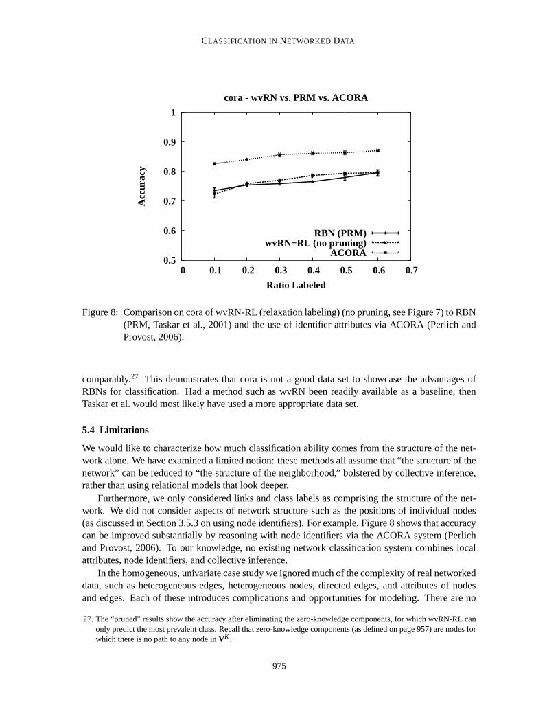
CLASSIFICATION IN NETWORKED DATA
0.5
0.6
0.7
0.8
0.9
1
0 0.1 0.2 0.3 0.4 0.5 0.6 0.7
Acc
urac
y
Ratio Labeled
cora - wvRN vs. PRM vs. ACORA
RBN (PRM)wvRN+RL (no pruning)
ACORA
Figure 8: Comparison on cora of wvRN-RL (relaxation labeling) (no pruning, see Figure 7) to RBN(PRM, Taskar et al., 2001) and the use of identifier attributes via ACORA (Perlich andProvost, 2006).
comparably.27 This demonstrates that cora is not a good data set to showcase the advantages ofRBNs for classification. Had a method such as wvRN been readily available as a baseline, thenTaskar et al. would most likely have used a more appropriate data set.
5.4 Limitations
We would like to characterize how much classification ability comes from the structure of the net-work alone. We have examined a limited notion: these methods all assume that “the structure of thenetwork” can be reduced to “the structure of the neighborhood,” bolstered by collective inference,rather than using relational models that look deeper.
Furthermore, we only considered links and class labels as comprising the structure of the net-work. We did not consider aspects of network structure such as the positions of individual nodes(as discussed in Section 3.5.3 on using node identifiers). For example, Figure 8 shows that accuracycan be improved substantially by reasoning with node identifiers via the ACORA system (Perlichand Provost, 2006). To our knowledge, no existing network classification system combines localattributes, node identifiers, and collective inference.
In the homogeneous, univariate case study we ignored much of the complexity of real networkeddata, such as heterogeneous edges, heterogeneous nodes, directed edges, and attributes of nodesand edges. Each of these introduces complications and opportunities for modeling. There are no
27. The “pruned” results show the accuracy after eliminating the zero-knowledge components, for which wvRN-RL canonly predict the most prevalent class. Recall that zero-knowledge components (as defined on page 957) are nodes forwhich there is no path to any node in VK .
975
MACSKASSY AND PROVOST
comprehensive, empirical machine learning studies that consider these dimensions systematically.For example, when using attributes of nodes, how much is gained by using them in the relationalclassifier, as opposed to using them simply to initialize priors? (For example, Chakrabarti et al.1998 found that using the text of hyperlinked documents reduced performance.) Similarly, howmuch value is added by considering multiple edge types explicitly?
An important limitation of this work, with respect to its relevance to practical problems, isthat we chose training data randomly to be labeled. It is likely that the data for which labels areavailable are interdependent. For example, all the members from one terrorist cell may be knownand none from another. If other attributes are available more uniformly, then studies such as thismay artificially favor network-only methods over attribute-based methods.
5.5 Conclusions and Future Work
We introduced a modular toolkit, NetKit-SRL, for classification in networked data. The importanceof NetKit is three-fold: (1) it generalizes several existing methods for classification in networkeddata, thereby making comparison to existing methods possible; (2) it enables the creation and use ofmany new algorithms by its modularity and extensibility, and (3) it enables the analysis/comparisonof individual components and configurations.
We then used NetKit to perform a case study of within-network, univariate classification forhomogeneous networked data. The case study makes several contributions. It provides demonstra-tive support for points 2 and 3 above. Of the five network classifiers that stood clearly above therest, three were novel combinations of components (and thus, novel relational classifiers). Certaincollective inference and relational classification components stood out with consistently better per-formance. For collective inference, relaxation labeling was best when there are few known labels;it mattered little which collective inference method is used when there were many known labels.For relational classification, the link-based classifier clearly was preferable when many labels wereknown. The lower-variance methods (wvRN and cdRN) dominated when fewer labels were known.In combination, two pairs of relational classifier/collective inference combinations stand out strik-ingly: nLB with any of the collective inference methods dominates when many labels are known;the relational neighbor methods with relaxation labeling (wvRN-RL and cdRN-RL) dominate whenfewer labels are known. Of particular relevance given this latter result, we also show the close cor-respondence of several simple, network classification methods: the node-centric wvRN-RL (Mac-skassy and Provost, 2003), the random-field method of Zhu et al. (2003), and classic connectionisttechniques such as Hopfield networks (Hopfield, 1982).
The case study demonstrates the power of simple network classification models, and arguesthat they must be included when evaluating relational learning methods on networked data. On thebenchmark data sets, error rates were reduced substantially by taking into account only the class-linkage structure of the network. Although learning helped in many cases, the no-learning wvRNwas a very strong competitor—performing very well especially when few labels were known. Thisresult was supported further by followup analyses showing cases where one would draw overly opti-mistic conclusions about the value of more-sophisticated methods if these network-only techniqueswere not used as baselines. It also raises the question of whether we need “better” benchmark datasets—to showcase the value of more-powerful techniques.
More generally, the results showcase two different modes of within-network classification thatcall for different types of methods: when many labels are known versus when few labels are known.
976

CLASSIFICATION IN NETWORKED DATA
These modes correspond to different application scenarios. The former may correspond (for ex-ample) to networks that evolve over time with new nodes needing classification before their labelsbecome known naturally, as would be the case for predicting movie box-office receipts. Examplesof the little-known scenario can be found in counter-terrorism and law enforcement, where analystsform complex interaction networks containing a few, known bad guys. The little-known scenariohas an economic component, similar to active learning: it may be worthwhile to incur costs to la-bel additional nodes in the network, because this will lead to much improved classification. Thissuggests another direction for future work—identifying the most beneficial nodes for labeling (cf.,Domingos and Richardson, 2001).
The case study also showcases a problem of representation for network classification: the se-lection of which edges to use. We show that edge selection can make a considerable difference,and suggest techniques analogous to those used in traditional feature selection. It is straightforwardto extend NetKit’s relational classification methods to handle heterogeneous links. However, thatwould not solve the fundamental problem that edge selection (like feature selection) may improvegeneralization performance, as well as provide simpler models.
Classification in networked data is important for real-world applications and presents manyopportunities for machine-learning research. The field is beginning to amass benchmark domainscontaining networked data. We hope that NetKit can facilitate systematic study.
Acknowledgments
David Jensen made many helpful suggestions, including pointing us to the WebKB data set andsuggesting ways to do well on it. Abraham Bernstein collaborated on the generation of the twoindustry classification data sets. Kaveh R. Ghazi worked diligently coding the open-source NetKitand ensuring that it would be ready for release on schedule. We thank Ben Taskar and Andrew Mc-Callum for providing us with versions of the cora data set. Thanks to Sugato Basu, Misha Bilenko,Avrim Blum, Pedro Domingos, Joydeep Ghosh, Michael Kearns, Yann LeCun, Andrew McCallum,Jennifer Neville, Mark Newman, Claudia Perlich, and audience members of talks for helpful com-ments and discussions. Finally, we thank Andrew McCallum and the anonymous reviewers whohelped to strengthen the paper considerably.
This work was funded in part by a grant from the New York Software Industry Association.This research also was sponsored in part by the Air Force Research Laboratory, Air Force MaterielCommand, USAF, under Agreement number F30602-01-2-0585. The views and conclusions con-tained herein are those of the authors and should not be interpreted as necessarily representing theofficial policies or endorsements, either expressed or implied, of AFRL or the U.S. Government.
References
J. C. Almack. The influence of intelligence on the selection of associates. School and Society, 16:529–530, 1922.
A. Bernstein, S. Clearwater, and F. Provost. The relational vector-space model and industry clas-sification. In Proceedings of the Learning Statistical Models from Relational Data Workshop atthe Nineteenth International Joint Conference on Artificial Intelligence (IJCAI), 2003.
977

MACSKASSY AND PROVOST
J. Besag. Spatial interaction and the statistical analysis of lattice systems. Journal of the RoyalStatistical Society, 36(2):192–236, 1974.
J. Besag. Statistical analysis of non-lattice data. The Statistician, 24(3):179–195, 1975.
J. Besag. On the statistical analysis of dirty pictures. Journal of the Royal Statistical Society, 48(3):259–302, 1986.
P. M. Blau. Inequality and Heterogeneity: A Primitive Theory of Social Structure. New York: FreePress, 1977.
A. Blum and S. Chawla. Learning from labeled and unlabeled data using graph mincuts. In Pro-ceedings of the Eighteenth International Conference on Machine Learning (ICML), pages 19–26,2001.
A. Blum, J. Lafferty, R. Reddy, and M. R. Rwebangira. Semi-supervised learning using random-ized mincuts. In Proceedings of the Twentyfirst International Conference on Machine Learning(ICML), pages 97–104, 2004.
H. Bott. Observation of play activities in a nursery school. Genetic Psychology Monographs, 4:44–88, 1928.
Y. Boykov, O. Veksler, and R. Zabih. Fast approximate energy minimization via graph cuts. IEEETransactions on Pattern Analysis and Machine Intelligence (PAMI), 23(11):1222–1239, 2001.
S. Chakrabarti, B. Dom, and P. Indyk. Enhanced hypertext categorization using hyperlinks. InProceedings of the 1998 ACM SIGMOD International Conference on Management of Data, pages307–319, 1998.
C. Cortes, D. Pregibon, and C. T. Volinsky. Communities of interest. In Proceedings of the FourthInternational Conference on Advances in Intelligent Data Analysis (IDA), pages 105–114, 2001.
R. G. Cowell, A. P. Dawid, S. L. Lauritzen, and D. J. Spiegelhalter. Probabilistic networks andexpert systems. Springer, 1999.
M. Craven, D. Freitag, A. McCallum, T. Mitchell, K. Nigam, and C. Y. Quek. Learning to ex-tract symbolic knowledge from the World Wide Web. In Proceedings of the Fifteenth NationalConference on Artificial Intelligence (AAAI), pages 509–516, 1998.
L. De Raedt, H. Blockeel, L. Dehaspe, and W. Van Laer. Three companions for data mining infirst order logic. In S. Dzeroski and N. Lavrac, editors, Relational Data Mining, pages 105–139.Berlin; New York: Springer, 2001.
I. S. Dhillon. Co-clustering documents and words using bipartite spectral graph partitioning. InProceedings of the Seventh ACM SIGKDD International Conference on Knowledge Discoveryand Data Mining, pages 269–274, 2001.
R. L. Dobrushin. The description of a random field by means of conditional probabilities andconditions of its regularity. Theory of Probability and its Applications, 13(2):197–224, 1968.
978

CLASSIFICATION IN NETWORKED DATA
P. Domingos and M. Richardson. Mining the network value of customers. In Proceedings of theSeventh ACM SIGKDD International Conference on Knowledge Discovery and Data Mining,pages 57–66, 2001.
S. Dzeroski and N. Lavrac. Relational Data Mining. Berlin; New York: Springer, 2001.
T. Fawcett and F. Provost. Adaptive fraud detection. Data Mining and Knowledge Discovery, 3:291–316, 1997.
T. Fawcett and F. Provost. Activity monitoring: Noticing interesting changes in behavior. In Pro-ceedings of the Fifth ACM SIGKDD International Conference on Knowledge Discovery and DataMining, pages 53–62, 1999.
P. A. Flach and N. Lachiche. Naive Bayesian classification of structured data. Machine Learning,57:233-269, 2004.
N. Friedman, L. Getoor, D. Koller, and A. Pfeffer. Learning probabilistic relational models. InProceedings of the Sixteenth International Joint Conference on Artificial Intelligence (IJCAI),pages 1300–1309, 1999.
A. Galstyan and P. Cohen. Is guilt by association a bad thing? In Proceedings of the First Interna-tional Conference on Intelligence Analysis (IA), 2005.
S. Geman and D. Geman. Stochastic relaxation, Gibbs distributions and the Bayesian restorationof images. IEEE Transactions on Pattern Analysis and Machine Intelligence (PAMI), 6:721–741,1984.
W. R. Gilks, S. Richardson, and D. J. Spiegelhalter. Markov Chain Monte Carlo in Practice. Chap-man & Hall/CRC, 1995.
D. Greig, B. Porteous, and A. Seheult. Exact maximum a posteriori estimation for binary images.Journal of the Royal Statistical Society, 51(2):271–279, 1989.
D. D. Heckathorn and J. Jeffri. Jazz networks: Using respondent-driven sampling to study stratifi-cation in two jazz musician communities. Unpublished paper presented at American SociologicalAssociation Annual Meeting, August 2003.
D. Heckerman, D. M. Chickering, C. Meek, R. Rounthwaite, and C. Kadie. Dependency networksfor inference, collaborative filtering, and data visualization. Journal of Machine Learning Re-search (JMLR), 1:49–75, 2000.
S. Hill, F. Provost, and C. Volinsky. Network-based marketing: Identifying likely adopters viaconsumer networks. Statistical Science, 22(2):256–276, 2006a.
S. Hill, D.K. Agarwal, R. Bell, and C. Volinsky. Building an effective representation for dynamicnetworks. Journal of Computational & Graphical Statistics, 15(3):584–608, 2006b.
G. E. Hinton and T. J. Sejnowski. Learning and relearning in Boltzmann machines. Parallel Dis-tributed Processing: Explorations in the Microstructure of Cognition, 1: Foundations:282–317,1986.
979

MACSKASSY AND PROVOST
J. J. Hopfield. Neural networks and physical systems with emergent collective computational abil-ities. Proceedings of the National Academy of Sciences of the United States of America, 79(8):2554–2558, 1982.
Z. Huang, H. Chen, and D. Zeng. Applying associative retrieval techniques to alleviate the sparsityproblem in collaborative filtering. ACM Transactions on Information Systems (TOIS), 22(1):116–142, 2004.
R. A. Hummel and S. W. Zucker. On the foundations of relaxation labeling processes. IEEETransactions on Pattern Analysis and Machine Intelligence (PAMI), 5(3):267–287, 1983.
E. Ising. Beitrag zur Theorie des Ferromagnetismus. Zeitschrift f. Physik, 31:253–258, 1925.[German].
D. Jensen and J. Neville. Data mining in social networks. In National Academy of Sciences Sympo-sium on Dynamic Social Network Modeling and Analysis, 2002a.
D. Jensen and J. Neville. Linkage and autocorrelation cause feature selection bias in relational learn-ing. In Proceedings of the Nineteenth International Conference on Machine Learning (ICML),pages 259–266, 2002b.
D. Jensen, J. Neville, and B. Gallagher. Why collective inference improves relational classification.In Proceedings of the Tenth ACM SIGKDD International Conference on Knowledge Discoveryand Data Mining, pages 593–598, 2004.
T. Joachims. Transductive learning via spectral graph partitioning. In Proceedings of the TwentiethInternational Conference on Machine Learning (ICML), pages 290–297, 2003.
J. Kleinberg and E. Tardos. Approximation algorithms for classification problems with pairwiserelations: Metric labeling and Markov random fields. In Proceedings of the Fortieth AnnualSymposium on Foundations of Computer Science (FOCS), pages 14–23, 1999.
R. Kohavi and G. John. Wrappers for feature subset selection. Artificial Intelligence, 97(1–2):273–324, 1997.
D. Koller and A. Pfeffer. Probabilistic frame-based systems. In Proceedings of the Fifteenth Na-tional Conference on Artificial Intelligence (AAAI), pages 580–587, 1998.
S. Kramer, N. Lavrac, and P. Flach. Propositionalization approaches to relational data mining. InS. Dzeroski and N. Lavrac, editors, Relational Data Mining, pages 262–291. Berlin; New York:Springer, 2001.
J. Lafferty, A. McCallum, and F. Pereira. Conditional random fields: Probabilistic models for seg-menting and labeling sequence data. In Proceedings of the Eighteenth International Conferenceon Machine Learning (ICML), pages 282–289, 2001.
P. Langley. Crafting papers on machine learning. In Proceedings of the Seventeenth InternationalConference on Machine Learning (ICML), pages 1207–1212, 2000.
980

CLASSIFICATION IN NETWORKED DATA
P. Lazarsfeld and R. K. Merton. Friendship as a social process: A substantive and methodologicalanalysis. In M. Berger, T. Abel, and C. H. Page, editors, Freedom and Control in Modern Society,pages 18–66. Van Nostrand, 1954.
C. P. Loomis. Political and occupational cleavages in a Hanoverian village. Sociometry, 9:316–3333, 1946.
Q. Lu and L. Getoor. Link-based classification. In Proceedings of the Twentieth InternationalConference on Machine Learning (ICML), pages 496–503, 2003.
S. A. Macskassy and F. Provost. A simple relational classifier. In Proceedings of the Multi-Relational Data Mining Workshop (MRDM) at the Ninth ACM SIGKDD International Conferenceon Knowledge Discovery and Data Mining, 2003.
S. A. Macskassy and F. Provost. Suspicion scoring based on guilt-by-association, collective infer-ence, and focused data access. In Proceedings of the First International Conference on Intelli-gence Analysis (IA), 2005.
A. McCallum, K. Nigam, J. Rennie, and K. Seymore. Automating the construction of internetportals with machine learning. Information Retrieval, 3(2):127–163, 2000.
M. McPherson, L. Smith-Lovin, and J. M. Cook. Birds of a feather: Homophily in social networks.Annual Review of Sociology, 27:415–444, 2001.
K. Murphy, Y. Weiss, and M. I. Jordan. Loopy belief-propagation for approximate inference: Anempirical study. In Proceedings of the Fifteenth Conference on Uncertainty in Artificial Intelli-gence (UAI), pages 467–475, 1999.
J. Neville and D. Jensen. Iterative classification in relational data. In Proceedings of the Workshopon Learning Statistical Models from Relational Data at the Seventeenth National Conference onArtificial Intelligence (AAAI), pages 13–20, 2000.
J. Neville and D. Jensen. Collective classification with relational dependency networks. In Pro-ceedings of the Multi-Relational Data Mining Workshop (MRDM) at the Ninth ACM SIGKDDInternational Conference on Knowledge Discovery and Data Mining, 2003.
J. Neville and D. Jensen. Dependency networks for relational data. In Proceedings of the FourthIEEE International Conference in Data Mining (ICDM), pages 170–177, 2004.
J. Neville and D. Jensen. Leveraging relational autocorrelation with latent group models. In Pro-ceedings of the Fifth IEEE International Conference in Data Mining (ICDM), pages 322–329,2005.
J. Neville and D. Jensen. Relational dependency networks. Journal of Machine Learning Research(JMLR), 8(Mar):653–692, 2007.
J. Neville, D. Jensen, L. Friedland, and M. Hay. Learning relational probability trees. In Proceedingsof the Ninth ACM SIGKDD International Conference on Knowledge Discovery and Data Mining,pages 625–630, 2003.
981

MACSKASSY AND PROVOST
J. Neville, O. Simsek, D. Jensen, J. Komoroske, K. Palmer, and H. Goldberg. Using relationalknowledge discovery to prevent securities fraud. In Proceedings of the Eleventh ACM SIGKDDInternational Conference on Knowledge Discovery and Data Mining, pages 449–458, 2005.
M. E. J. Newman. Mixing patterns in networks. Physical Review E, 67, 2003. 026126.
J. Pearl. Probabilistic Reasoning in Intelligent Systems. Morgan Kaufmann, 1988.
C. Perlich. Citation-based document classification. In Workshop on Information Technology andSystems (WITS), 2003.
C. Perlich and F. Provost. Aggregation-based feature invention and relational concept classes. InProceedings of the Ninth ACM SIGKDD International Conference on Knowledge Discovery andData Mining, pages 167–176, 2003.
C. Perlich and F. Provost. Distribution-based aggregation for relational learning with identifierattributes. Machine Learning, 62(1/2):65–105, 2006.
C. Perlich, F. Provost, and J. Simonoff. Tree induction vs. logistic regression: A learning-curveanalysis. Journal of Machine Learning Research (JMLR), 4:211-255, 2003.
A. Popescul and L. H. Ungar. Statistical relational learning for link prediction. In Proceedings ofthe Learning Statistical Models from Relational Data Workshop at the Nineteenth InternationalJoint Conference on Artificial Intelligence (IJCAI), 2003.
R. B. Potts. Some generalized order-disorder transformations. Cambridge Philosophic Society, 48:106–109, 1952.
H. M. Richardson. Community of values as a factor in friendships of college and adult women.Journal of Social Psychology, 11:303–312, 1940.
M. Richardson and P. Domingos. Markov logic networks. Machine Learning, 62(1/2):107–136,2006.
J. Rocchio. Relevance feedback in information retrieval. In G. Salton, editor, The SMART RetrievalSystem: Experiments in Automatic Document Processing, chapter 14, pages 313–323. Prentice–Hall, 1971.
A. Rosenfeld, R. Hummel, and S. Zucker. Scene labeling by relaxation operations. IEEE Transac-tions on Systems, Man and Cybernetics, 6:420–433, 1976.
L. J. Savage. The Foundations of Statistics. John Wiley and Sons, 1954.
E. Segal, H. Wang, and D. Koller. Discovering molecular pathways from protein interaction andgene expression data. Bioinformatics, 19:I264–I272, Jul 2003a.
E. Segal, R. Yelensky, and D. Koller. Genome-wide discovery of transcriptional modules from DNAsequence and gene expression. Bioinformatics, 19:I273–I282, Jul 2003b.
B. Taskar, P. Abbeel, and D. Koller. Discriminative probabilistic models for relational data. InProceedings of the Eighteenth Conference on Uncertainty in Artificial Intelligence (UAI), pages485–492, 2002.
982

CLASSIFICATION IN NETWORKED DATA
B. Taskar, E. Segal, and D. Koller. Probabilistic classification and clustering in relational data. InProceedings of the Seventeenthth International Joint Conference on Artificial Intelligence (IJ-CAI), pages 870–878, 2001.
B. Taskar, V. Chatalbashev, and D. Koller. Learning associative Markov networks. In Proceedingsof the Twentyfirst International Conference on Machine Learning (ICML), 2004.
K. Tumulty. Inside Bush’s Secret Spy Net [electronic version]. Time, 167(21), 2006. RetrievedMay 25, 2006, from http://www.time.com/time/archive/preview/0,10987,1194021,00.html.
V. N. Vapnik. The support vector method of function estimation. In J. Suykens and J. Vandewalle,editors, Nonlinear Modeling: Advanced Black-Box Techniques, pages 55–86. Kluwer, Boston,1998a.
V. N. Vapnik. Statistical Learning Theory. John Wiley, NY, 1998b.
M. J. Wainwright and M. I. Jordan. Graphical models, exponential families, and variational infer-ence. Technical Report 649, University of California, Berkeley, 2003.
G. Winkler. Image Analysis, Random Fields and Markov Chain Monte Carlo Methods. Springer-Verlag, 2nd edition, 2003.
I. H. Witten and E. Frank. Data Mining: Practical Machine Learning Tools with Java Implementa-tions. Morgan Kaufmann, San Francisco, 2000.
X. Zhu, Z. Ghahramani, and J. Lafferty. Semi-supervised learning using Gaussian fields and har-monic functions. In Proceedings of the Twentieth International Conference on Machine Learning(ICML), pages 912–919, 2003.
983