classification of solutions of the forced periodic nonlinear …vered/publistorder/r37_non10... ·...

Classification of solutions of the forced periodic nonlinear Schrödinger equation

This article has been downloaded from IOPscience. Please scroll down to see the full text article.

2010 Nonlinearity 23 2183

(http://iopscience.iop.org/0951-7715/23/9/008)

Download details:

IP Address: 132.77.4.43

The article was downloaded on 31/08/2010 at 12:52

Please note that terms and conditions apply.

View the table of contents for this issue, or go to the journal homepage for more

Home Search Collections Journals About Contact us My IOPscience

http://iopscience.iop.org/page/terms

http://iopscience.iop.org/0951-7715/23/9

http://iopscience.iop.org/0951-7715

http://iopscience.iop.org/

http://iopscience.iop.org/search

http://iopscience.iop.org/collections

http://iopscience.iop.org/journals

http://iopscience.iop.org/page/aboutioppublishing

http://iopscience.iop.org/contact

http://iopscience.iop.org/myiopscience

IOP PUBLISHING NONLINEARITY

Nonlinearity 23 (2010) 2183–2218 doi:10.1088/0951-7715/23/9/008

Classification of solutions of the forced periodicnonlinear Schrodinger equation

Eli Shlizerman1 and Vered Rom-Kedar2

Faculty of Mathematics and Computer Science, The Weizmann Institute of Science, Rehovot,76100, Israel1From 1 Sep 2009 affiliated with the Department of Applied Mathematics, University ofWashington, Seattle, WA 98195, USA2 The Estrin family chair of Computer Science and Applied Mathematics

E-mail: [email protected] and [email protected]

Received 14 July 2009, in final form 30 April 2010Published 10 August 2010Online at stacks.iop.org/Non/23/2183

Recommended by D V Treschev

AbstractThe integrable structure of the periodic one-dimensional nonlinear Schrodingerequation is utilized to gain insights regarding the perturbed near-integrabledynamics. After recalling the known results regarding the structure andstability of the unperturbed standing and travelling waves solutions, two newstability results are presented: (1) it is shown numerically that the stabilityof the ‘outer’ (cnoidal) unperturbed solutions depends on their power (the L2

norm): they undergo a finite sequence of Hamiltonian–Hopf bifurcations astheir power is increased. (2) another proof that the ‘inner’(dnoidal) unperturbedsolutions with multiplicity �2 are linearly unstable is presented. Then, to studythe global phase-space structure, an energy–momentum bifurcation diagram(PDE-EMBD) that consists of projections of the unperturbed standing andtravelling waves solutions to the energy–power plane and includes informationregarding their linear stability is constructed. The PDE-EMBD helps us toclassify the behaviour near the plane wave solutions: the diagram demonstratesthat below some known threshold amplitude, precisely three distinct observablechaotic mechanisms arise: homoclinic chaos, homoclinic resonance and, forsome parameter values, parabolic-resonance. Moreover, it appears that thedynamics of the PDE chaotic solutions that exhibit the parabolic-resonanceinstability may be qualitatively predicted: these exhibit the same dynamicsas a recently derived parabolic-resonance low-dimensional normal form. Inparticular, these solutions undergo adiabatic chaos: they follow the level linesof an adiabatic invariant till they reach the separatrix set at which the adiabaticinvariant undergoes essentially random jumps.

Mathematics Subject Classification: 35Q55, 70H11, 37Kxx

(Some figures in this article are in colour only in the electronic version)

0951-7715/10/092183+36$30.00 © 2010 IOP Publishing Ltd & London Mathematical Society Printed in the UK & the USA 2183

http://dx.doi.org/10.1088/0951-7715/23/9/008

mailto: [email protected]

mailto: [email protected]

http://stacks.iop.org/no/23/2183

2184 E Shlizerman and V Rom-Kedar

1. Introduction

The one-dimensional nonlinear Schrodinger (NLS) equation is an integrable partial differentialequation possessing an infinite number of symmetries corresponding to infinite number ofconserved quantities. Indeed, utilizing the inverse scattering theory the one-dimensionalNLS [1, 17, 42, 45] (on the line R or the circle T

1) is solvable as an initial value problem.In the physical context, the NLS equation is a first order nonlinear model for the propagationof dispersive waves that interact nonlinearly and thus arises in various applications such aspropagation of laser beams in optical fibres, surface waves and Bose–Einstein condensates.The role of the nonlinear terms has become especially significant in recent years, as highintensity laser beams [45] and Bose–Einstein condensates are realized experimentally [21].The common nonlinearity for the NLS equation is the cubic nonlinearity and the sign of thenonlinearity (sign (g) in equation (1.1)) determines its nature3: a defocusing equation for g < 0and a focusing equation for g > 0:

iϕt − ϕxx − g|ϕ|2ϕ = 0. (1.1)

From the variety of solutions of the integrable one-dimensional NLS equation the solutionsthat attracted much attention of analytical, numerical and experimental studies are the standingwaves or their generalization—the travelling waves (on R, the famous solitary waves solutionscorrespond to the subclass of such waves having a finite ‘power’, namely a finite L2 norm)[3, 45]. The standing waves are solutions that are stationary in the spatial domain and periodicin time. The travelling waves have a fixed spatial profile that periodically oscillates in time andmoves with a constant velocity in the spatial domain. The existence of stable standing/travellingwaves is of high practical importance, for example for encoding and transmitting data in opticalfibres [2, 44].

The linearization of the NLS equation about a standing wave solution boils down tosolving the eigenvalue problem of a matrix operator N (see [55] and section 2.2). Althoughthe linearized operator consists of two self-adjoint operators L+ and L−, it is not self-adjointand determining its eigenvalues is not a straightforward task. The linearized problem near thequiescent and the plane wave solutions is explicitly solvable by modulation stability analysis.In particular, as the amplitude of the plane wave grows, more modes become unstable, andthe number of linearly unstable modes (LUMs) for a given plane wave amplitude may beexplicitly computed (see [17] and section 2.2). The ground state standing waves on R

N wereproved to be nonlinearly stable by utilizing the framework developed by [9, 16] for the KdVequation and by [57] for the NLS equation. To deal with the other standing waves, a theoreticalframework for proving linear instability was developed in [28–30, 36]. In this framework onededuces instability when the number of positive eigenvalues of the operator L+ exceeds thenumber of positive eigenvalues of the operator L− by more than one (see section 2.2). Recently,these theories were applied to the one-pulse and two-pulse dnoidal standing waves of the one-dimensional NLS with periodic boundary conditions [6] and extended to provide counting ofthe number of unstable eigenvalues [33].

Here we consider this latter case of the focusing cubic one-dimensional NLS equationwith periodic boundary conditions. The infinite-dimensional phase space is composed of levelsets of the constants of motion. A level set corresponds generically to one or several infinite-dimensional tori. A solution of the NLS equation belonging to a generic regular level setis a quasi-periodic solution winding on a torus and can be decomposed into infinite set ofaction-angle coordinates. Each action-angle pair (a degree of freedom) can be considered as

3 We keep the parameter g, which may be scaled out, to ease the comparison with previous works on the focusingequation in which g is taken to be either 1 or 2.

Classification of solutions of the forced periodic nonlinear Schrodinger equation 2185

an oscillator and corresponds to an invariant of the integrable equation. The non-genericsingular level sets may be composed of finite-dimensional tori (these may be viewed asdegenerate infinite-dimensional tori) and possibly their stable and unstable manifolds (thelinearized operator at the degenerate tori determines their linear stability). An example forsuch a singular level set is the one corresponding to standing/travelling wave solutions: then thedegenerate torus is a circle. Indeed, standing and travelling waves were shown to exist in thefocusing cubic NLS with periodic boundary conditions. In fact, these solutions can be foundanalytically, since they correspond to periodic solutions of the Duffing equation (see [6, 55]and section 2.1). These solutions become unstable as their amplitude increases and additionalstanding/travelling waves bifurcate from them (see [6, 24, 25, 33] and section 2.2). Note thatdue to integrability, even in the unstable cases, the solutions near the unstable waves are regular,namely quasi-periodic (see section 2.3).

In applications, the one-dimensional NLS appears only as a leading order approximation,and thus it is natural to consider the effect of small correction terms and forcing. The inclusionof such terms typically breaks the integrable structure [14]. If the forcing and correctionterms are small, one may hope to be able to analyse the near-integrable PDE by perturbativemethods. To study such systems, it was proposed to consider the simplest possible prototypicalperturbations—spatially independent time-periodic forcing and damping [15, 17]:

iϕt − ϕxx − g|ϕ|2ϕ = ε exp(−i�2t + iα) − iδϕ, ϕ0(x) = ϕ(x, 0). (1.2)

Here ε is the small forcing amplitude, δ is the small damping coefficient (so, hereafter,ε, δ � 1), �2 is the forcing frequency and α is an arbitrary phase. Following [55], it iseasy to show that for all ϕ0 ∈ H1(T) there exist a unique ϕ ∈ C([0, ∞), H1(T)) that solvesthe initial value problem of equation (1.2).

A natural question that arises is how to characterize the solutions of the perturbed equation.Obtaining a complete infinite-dimensional phase space description of a non-integrable PDEwhich is not strongly dissipative appears to be too difficult. Traditionally, the structure of thephase space had been interpreted only near special solutions, usually only near the quiescentsolution. For the near-integrable NLS equation, utilizing the known integrable phase-spacestructure near finite amplitude solutions such as standing/travelling waves, one may explorelarger regions in the infinite-dimensional phase space. Indeed it was proposed that in thenear-integrable setting, solutions with initial data near unstable standing wave solutions of theintegrable equation may become irregular [13].

To gain intuition regarding the different mechanisms of irregularities in the near-integrablesystem when the plane wave has at most one LUM, a two-mode Galerkin truncation of theperturbed NLS was introduced [10–12, 17]. The unperturbed truncated system turned out tobe a two degrees of freedom Hamiltonian system, with an additional integral of motion. Thesetwo integrals of motion were found to correspond to the first two invariants of the unperturbedPDE: the energy and the power (the L2 norm) of the solutions. As usual, most level setsof the two degree of freedom Hamiltonian correspond to one or two invariant two-tori. Thespatial independent solutions of the NLS, the plane waves, appear as singular level sets, namelyinvariant circles of both the truncated and full PDE model. As their amplitudes increase thesecircles become normally unstable, and families of homoclinic orbits are created in both the ODEand the PDE models, leading to the creation of homoclinic chaos in the perturbed equation [23].When the plane wave is both unstable and resonant, a novel mechanism of instability emerges—the hyperbolic resonance [31, 38]. New methodologies and tools introduced to this PDE–ODEstudy had finally led to a proof that the homoclinic resonance dynamics has analogous behaviourin the PDE setting [17, 32, 43]. To fully classify the near-integrable structure of the truncatedmodel for all parameters k, �, the hierarchy of bifurcations framework was developed [51].


The analysis showed that when the spatial box length and the frequency are close to theparticular relation �2 = �2

pr = k2/2 where k = 2π/L, the truncated NLS admits a new typeof chaotic dynamics—parabolic resonant solutions (see [49] and section 3.3). In [52] it wasdemonstrated that analogous chaotic trajectories appear in the PDE setting.

Going beyond the two degrees of freedom regime, it was shown that in the dissipative case,when the resonant plane wave amplitude is increased so it has two or more LUMs, solutions withinitial data near the plane wave evolve chaotically in both time and space so that their spatialcoherence is lost—such solutions were called spatio-temporal chaotic (STC) [18]. Recently,we demonstrated that in the Hamiltonian case, the parabolic-resonance mechanism enables todrive solutions with small initial data (near the unperturbed stable plane wave) into STC withsmaller forcing amplitude than the forcing amplitude needed to drive such data to STC in theelliptic or hyperbolic resonance cases [53].

In this paper, we propose that a specific bifurcation diagram, the PDE-EMBD is beneficialin studying how the infinite-dimensional integrable phase-space structure deforms when smallperturbations are applied. The first part of the paper is devoted to constructing the diagram,namely studying the integrable structure (including some new results regarding the stability ofsome of the standing waves) whereas the second part is devoted to studying the near-integrabledynamics (including some new results regarding the parabolic-resonance mechanism). Morespecifically, in section 2 we review the relevant properties of the integrable periodic one-dimensional NLS, provide the analytic expressions for the standing and travelling wavessolutions and study their stability. These results are then used for constructing the PDE-EMBD.In section 3 we employ this construction to analyse the dynamics near-plane waves of the near-integrable forced NLS. We review the known properties of such perturbed solutions and analysethe parabolic-resonance mechanism that was identified in the PDE in [52] and was describedas a route from stability to spatio-temporal chaos in [53].

2. The unperturbed problem

2.1. Standing and travelling wave solutions

2.1.1. General properties. Consider the autonomous one-dimensional NLS equation withperiodic boundary conditions (substituting in (1.2) ϕ = ψ exp(−i�2t + iα), and settingε = δ = 0):

i�t = �xx + (g|�|2 − �2)�, (2.1)

�(x, 0) = �0(x),

where �(x, t) = �(x + L, t), x ∈ R, g = 2 and �0(x) ∈ Hr (T), r � 3 (we will mostlyconsider the two-mode analytic initial data, see section 3) denotes the initial data profile. TheNLS equation is integrable: it is completely solvable by the inverse scattering technique [42]and, for smooth initial data, it has an infinite number of constants of motion. The first threeconserved quantities, ordered by the required number of spatial derivatives are

Particle number : I (�) = 1

L

∫ L/2

−L/2|�|2 dx, (2.2)

Linear momentum : P(�) = 1

2iL

∫ L/2

−L/2�∂x�

∗ − �∗∂x� dx, (2.3)

Hamiltonian : H0(�) = 1

L

∫ L/2

−L/2

(−|∂x�|2 +

g

2|�|4 − �2|�|2

)dx. (2.4)


These correspond to the conservation of mass, linear momentum and energy and can be easilyshown to be invariants of the equation. Other conserved quantities involve higher spatialderivatives of the solution. The corresponding symmetries to equations (2.2)–(2.4) are phasetranslation, space translation and time translation (the Galilean transformation).

Thus if �(x, t) is a solution of the NLS then so is the three-parameter family of solutions� ′(x, t; v, s, θ):

x ′ = x − vt + s, (2.5)

� ′(x, t; v, s, θ) = �(x ′, t) exp

[i

(−v

2x +

v2

4t + θ

)]. (2.6)

The same transformation applies to the periodic case, yet the periodic boundary conditionsimpose a quantization on the values of v

vj = 4π

Lj, j ∈ Z,

whereas s, θ remains arbitrary.

2.1.2. Standing waves. The standing waves are oscillatory in time separable solutions of theintegrable NLS equation

�sw(x, t) = e−iEλt+iE0�Eλ(x), (2.7)

where Eλ, �Eλ(x) are eigenvalues and eigenfunctions of the nonlinear operator N :

N (�Eλ)�Eλ

= (∂xx + g|�Eλ|2 − �2)�Eλ

= Eλ�Eλ, (2.8)

�Eλ(x + L) = �Eλ

(x). (2.9)

Multiplying by �∗Eλ

and integrating, the eigenvalue Eλ and the integral K , are defined by

Eλ = K(�Eλ)/I (�Eλ

), (2.10)

K(�) = 1

L

∫ L/2

−L/2(−|∂x�|2 + g|�|4 − �2|�|2) dx. (2.11)

The linear momentum of the standing waves always vanishes, P(�sw) = 0. In general, thecalculation of eigenvalues and eigenfunctions of nonlinear operators is a formidable task.However, for real �Eλ

(x), equation (2.8) corresponds to the Duffing equation:

∂xx�Eλ+ g�3

Eλ− (Eλ + �2)�Eλ

= 0, (2.12)

and its general solutions are explicitly given by Jacobi-elliptic functions (see [6] and below).Figure 1 shows the corresponding phase-portrait (�Eλ

, ∂x�Eλ) of the Duffing equation for

a fixed Eλ. There are different families of solutions: stable and unstable fixed points,homoclinic orbits4, solutions inside the homoclinic orbit—inner solutions and solutions outsideof the homoclinic orbit—outer solutions. Next we show that imposing the periodic boundaryconditions selects a discrete set of Duffing solutions that are either fixed points, periodic innersolutions or periodic outer solutions.

The quiescent fixed point (black), (�Eλ, ∂x�Eλ

) = (0, 0), is a saddle (center) whenEλ > −�2 (respectively when Eλ < −�2). In the first case, the saddle has two homoclinicorbits that enclose the two stable fixed points (blue), (�Eλ

, ∂x�Eλ) = (±

√Eλ + �2/g, 0).

4 these are the celebrated soliton solutions on the infinite line.


–3 –2 –1 0 1 2 3

–5

–4

–3

–2

–1

0

1

2

3

4

5

ΨE

λ

∂ x Ψ

E

Figure 1. Phase space of the Duffing equation for g = 1, �2 = 1, L = 2π and Eλ = 3. The fixedpoints on the x-axis (blue) correspond to the NLS plane wave solutions (±

√(Eλ + �2)/g, 0). The

NLS L-periodic inner solutions �intj (x) and outer solutions �out

j (x) are marked in bold green andbold red, respectively.

These two centres correspond to the plane wave solutions of the NLS equation: they arespatially independent solutions, having a constant amplitude, �

pwEλ

(x) = |c|, and thus

�pw(x, t) = |c|eiγ (t) = |c|e−iEpwλ t+iE0 (2.13)

where from (2.2), (2.4) and (2.10) the phase velocity and the constants of motion of the planewave are

Epwλ (|c|; g, �2) = −�2 + g|c|2, I pw = |c|2 = (E + �2)

g, H

pw0 = g

2I 2 − �2I.

(2.14)

The general outer solutions of the Duffing equation are found in terms of the Jacobi-ellipticfunctions:

�outEλ,κ

(x) = a2

√2κ2

gcn(a2x, κ), a2 = 2π

L

√Eλ + �2

2κ2 − 1, (2.15)

∂x�outEλ,κ

(x) = −a22

√2

g

κ2L

2πsn(a2x, κ) dn(a2x, κ),

and their (spatial) period is

Lout(κ, Eλ + �2) = 4

√2κ2 − 1

Eλ + �2K(κ),

where K(κ) is the Jacobi complete elliptic integral of the first kind. Since the standing wavesolutions must be L-periodic, the condition

Lout(κ, Eλ + �2)

∣∣∣∣κ=κj

= L

j, j ∈ N (2.16)

leads to a selection, for any given Eλ, of a finite number of values κj (Eλ) at which the spatial-period satisfies this ‘quantization’ rule, see bold (red) curves outside the homoclinic orbit in


–3 –2 –1 0 1 2 3

–2

–1.5

–1

–0.5

0

0.5

1

1.5

2

Φ

x

Figure 2. Three different types of standing waves profiles. Solutions of equation (2.12) at �2 = 1,with Lint,out(k, Eλ) = L and I (�pw,int,out) = 1 are shown. The flat plane wave profile �pw(x) ismarked by a dashed (blue) line. The standing wave profile �int

1 (x) is marked by a solid (green)line and the profile �out

1 (x) is marked by a dashed–dotted (red) line.

figure 1 and the dotted dashed (red) curve in figure 2. Since ∂Lout/∂k �= 0 by the implicitfunction theorem the elliptic modulus κj (Eλ) is a function of the variable Eλ and can be foundby solving the equation Lout = L/j .

For small κ and negative Eλ + �2, �outEλ,κ

(x) is well approximated by the solutions to thelinearized equation near the quiescent solution:

�outEλ,κ

(x) −−−→κ → 0

�linEλ

(x) = cos (√

−(Eλ + �2)x + θ), (2.17)

where �linEλ

(x) solves the ‘linear standing wave’ equation

∂xx�linEλ

− (Eλ + �2)�linEλ

= 0. (2.18)

These linear solutions are L (in fact L/j ) periodic when Eλ = Eoutλ,j :

Eoutλ,j = −�2 −

(2πj

L

)2

(2.19)

and the discrete set of outer j oscillatory solutions asymptotes to these linear solutions in thesmall amplitude limit:

�outj (x; Eλ) := �out

Eλ,κj (Eλ)(x) −−−−−−−−−−−−−→

κj → 0, Eλ → Eλ,j�lin

Eλ,j(x). (2.20)

Similarly, the inner Lint periodic solutions (bold (green) curves inside the homoclinic orbit infigure 1 and solid (green) curve in figure 2) are

�intEλ,κ

(x) = a1

√2

gdn(a1x, κ), a1 = 2π

L

√Eλ + �2

(2 − κ2), (2.21)

∂x�intEλ,κ

(x) = −a21

√2

g

κ2L

2πsn(a1x, κ) cn(a1x, κ),

where κ = κ(Eλ) is the elliptic modulus of the solution, with period Lint(κ, Eλ + �2)

Lint(κ, Eλ + �2) = 2

√2 − κ2

Eλ + �2K(κ). (2.22)


As for the outer solutions, the elliptic modulus is determined by solving the equationLint = L/j . As κ → 0, the inner solutions �int

Eλ,κ(x) asymptote to the linear solution around

the plane wave solution. Requiring Lint(κj (Eλ), Eλ + �2) = L/j , the j -pulse branches aredefined as

�intj (x; Eλ) := �int

Eλ,κj (Eλ)(x) −−−−−−−−−−−−−→

κj → 0, Eλ → Eλ,j

�pwEλ,j

(x) + �linEλ,j

(x), (2.23)

where �linEλ,j

(x) = �linE

pwλ

(x) so the L/j periodicity implies

Eλ,j = −�2 +1

2

(2πj

L

)2

. (2.24)

Summarizing, there are two sets of families of L periodic j -oscillatory solutions: the outerfamilies �out

j (x; Eλ) that have 2j zeroes in a period, and the inner solutions, �intj (x; Eλ) that do

not change their sign (hereafter, when there is no ambiguity, we omit the explicit dependenceof these solutions on Eλ and denote �

int,outj (x) = �

int,outj (x; ·)).

2.1.3. Travelling waves. Applying the symmetry group transformation (equation (2.6)) tothe standing waves solutions �(x, t) = �Eλ

(x)e−iEλt , where �Eλis either a plane wave, an

interior or an exterior L-periodic solution) produces three-parameter families of travellingwaves solutions where the parameter v, the speed of the travelling wave, is discrete, and s andθ , its space and phase shifts, are continuous. To determine the corresponding eigenvalues ofthe travelling waves, we note that if one defines � ′(x, t; vj , s, θ) = �′

E′λ(x ′)e−iE′

λt where

E′λ = Eλ − v2

j

4. (2.25)

then �′ satisfies equation (2.8) with x ′ and E′λ replacing x and Eλ. Regarding the other

constants of motion, the transformation preserves the L2-norm

I (� ′(x, t; vj , s)) = I (�(x, t)) (2.26)

yet changes the Hamiltonian

H0(�′(x, t; vj , s)) = H0(�(x, t)) − vj

2

4I (�(x, t)), (2.27)

and the linear momentum

P(� ′(x, t; vj , s)) = −vj

2I (�(x, t)). (2.28)

2.2. Stability

Linearization about the standing wave solutions leads to the equation

iξt = ξxx − (Eλ + �2)ξ + g(2�2Eλ

(x)ξ + �2Eλ

(x)ξ ∗), (2.29)

where ξ is the perturbation and ξ ∗ denotes the complex conjugate of ξ . The dependence ofξ on time (oscillatory, exponentially increasing/decreasing) determines the linear stability of�Eλ

. For a general standing wave solution, equation (2.29) can be rewritten as [30, 35, 36]

i(ξ − ξ ∗)t = L+(ξ + ξ ∗), (2.30)

i(ξ + ξ ∗)t = L−(ξ − ξ ∗).


The operators L+ and L− are of Hill’s type—these are second order differential operators withperiodic potential and periodic boundary conditions

L+ : L+[x, �Eλ(x)]u = (∂xx − (Eλ + �2) + 3g�2

Eλ(x))u,

u(−L/2) = u(L/2), u′(−L/2) = u′(L/2),

L− : L−[x, �Eλ(x)]v = (∂xx − (Eλ + �2) + g�2

Eλ(x))v,

v(−L/2) = v(L/2), v′(−L/2) = v′(L/2).

The transformation ξ = u + iv brings equation (2.30) to a matrix form:(u

v

)t

=(

0 L−−L+ 0

) (u

v

)= N

(u

v

). (2.31)

This system is a Hamiltonian system that can be written in the form(u

v

)t

=(

0 1−1 0

) (L+ 00 L−

) (u

v

)= JH ′′

Eλ

(u

v

), (2.32)

where for a functional F(u, v) the notation F ′′(�Eλ) denotes the Hessian matrix D2F(u, v) at

u = �Eλand v = 0. Then H ′′

Eλ(�Eλ

) = H ′′0 (�Eλ

) − EλI′′(�Eλ

) is defined as the Hessian ofthe energy or the ‘linearized Hamiltonian’, where I and H0 are defined by equations (2.2) and(2.4), respectively.

The eigenvalues iωj of the operator N ,

N

(u

v

)= iω

(u

v

), (2.33)

determine the stability of the particular standing wave. Since the spectrum of N is symmetric5

the existence of a non-trivial eigenvalue with a real part (i.e. Im(ωj ) �= 0) implies that thestanding wave is unstable. Next we repeat, for completeness, the standard calculation of theeigenvalues and the eigenfunctions of N for the spatially independent quiescent and plane wavesolutions. For the other, spatially dependent standing waves, this calculation is too difficult andthe explicit solution of the eigenvalue problem is not known. For the inner solutions family,the theory of linear instability [30, 36] and orbital stability of [9, 16, 57] has recently beenextended to the periodic problem to establish when they are linearly stable/unstable withoutexplicitly calculating the spectrum of N [5, 6]. The main steps for establishing these resultsare included. The stability of the outer solutions family is found by numerical methods asexplained below.

2.2.1. Stability of the quiescent solution. The linearization (2.30) around the quiescentsolution �0(x) = 0, Eλ = 0,

iξt = ξxx − �2ξ (2.34)

is solved by ξ(x, t) = ξ (2πj/L)ei( 2πj

Lx+ωt) where j ∈ Z. The eigenvalue problem (2.31) for

the operator N is

det(N − iωI) =

−iω −�2 −

(2πj

L

)2

�2 +

(2πj

L

)2

−iω

= 0 (2.35)

5 The complex (respectively real) eigenvalues of N come in quadruples (respectively pairs when b = 0): iω1,2,3,4 =±a ± ib.


and together with (2.34) leads to the dispersion relation

ω2j =

((2πj

L

)2

+ �2

). (2.36)

The eigenvalues iωj are always pure imaginary and thus the quiescent solution is linearly

stable. The corresponding resonant eigenfunctions �(x, t) = ξ (2πj/L)ei( 2πj

Lx+ωj t)+iE0 are

exactly the linear modes �linEλ,j

that solve equation (2.18) and satisfy Eλ,j = −ωj . From thesecountable infinity linear eigenmodes that are associated with the discrete negative eigenvaluesEλ,j emanate the plane wave branch at j = 0 and, for j �= 0, the discrete set of the outersolutions �out

Eλ,κj (x) −−−−→κj → 0

�linEλ,j

(x), see figure 4.

2.2.2. Stability of the plane wave solution. The linearization (2.30) around the plane wavesolution �pw = |c|e−iEpw

λ t+iE0

iξt = ξxx + 2g|c|2ξ + g|c|2ξ ∗ (2.37)

leads to the eigenvalue problem (2.31) for the operator N :

det(N − iωI) =

−iω −(E

pwλ + �2) −

(2πj

L

)2

+ g|c|2

(Epwλ + �2) +

(2πj

L

)2

− 3g|c|2 −iω

(2.38)

=

−iω −

(2πj

L

)2

(2πj

L

)2

− 2g|c|2 −iω

= 0, (2.39)

which in turn leads to the dispersion relation:

ω2j =

(2πj

L

)2((

2πj

L

)2

− 2g|c|2)

. (2.40)

Hence, for (2πj/L)2 < 2g|c|2 the plane wave solution is unstable. More generally, planewaves with amplitude |c|2 in the range

Ipw = |c|2 ∈ 1

2g

(2π

L

)2

(j 2, (j + 1)2) = (IjLUM, I(j+1)LUM) (2.41)

have j LUM. Namely, the number of linear unstable modes grows linearly with the amplitude.Such instability is called ‘Benjamin–Feir instability’ in the dispersive wave community [8] and‘modulation instability’ in the plasma physics community [34]. In particular, we will see thatfor studying the perturbed dynamics it is important to note that for Ipw ∈ (0, I1LUM) the planewave is linearly stable, for Ipw ∈ (I1LUM, I2LUM) the plane wave has only one unstable mode,whereas for Ipw > I2LUM the plane wave has at least two unstable modes. Numerically, thelinearly stable plane wave solution in the region Ipw ∈ (0, I1LUM) appears to be also nonlinearlystable. Analytically, the study of nonlinear stability is beyond the scope of this work; however,it may be studied using methods similar to methods used in the proof of proposition 3.1 in [4],where nonlinear stability of plane wave solutions for the KdV equation was established.

At the bifurcation values IjLUM = (1/2g)(2π/L)2j 2, where Epwλ,j = −�2 + 1

2

(2πL

)2j 2,

two important structural changes occur in the vicinity of the plane wave branch; first, the interior


linear modes bifurcate from the plane wave family and become the discrete set of the innersolutions branches: �int

j (x; Eλ) −−−−−−−→Eλ → Eλ, j

�pwEλ,j

(x) + �linEλ,j

(x). Second, homoclinic orbits

to the plane wave are created. These orbits are solutions, �hom(x, t), of the integrable NLSequation such that �hom(x, t) → �pw(t) exponentially as t → ±∞. The analytic expressionfor these homoclinic orbits may be found via Backlund transformation [17, 23], and theirform becomes more and more complex as j , the number of LUMs, increases. Numerically,the structure of these orbits may be observed by computing quasi-periodic trajectories that areinitialized sufficiently close to the plane wave and thus ‘shadow’ the homoclinic structure [17].Figure 8(c) presents a quasi-periodic solution that shadows a 1-pulse homoclinc orbit of a1-LUM plane wave solution.

2.2.3. Stability of the inner (dnoidal) solutions. It was recently established that the innerstanding wave solutions �int

j (x) (solutions with j multiplicity such that their period Lint = L/j ,j ∈ N) are stable when j = 1 and are unstable when j = 2:

Theorem 1 ([6]). The inner standing wave solution �intj (x) with multiplicity j = 1 is orbitally

stable, i.e. the orbit O�int1

= ‖eiθ�int1 (· + y) : (y, θ) ∈ R × [0, 2π)‖ is nonlinearly stable. On

the other hand, �int2 (x) is linearly unstable.

Below, the instability of �int2 (x) is established in a slightly different way: instead of solving

explicitly the eigenvalue problem for the operator L+[x, �intj (x)] (as in theorem 3.1 of [6]) we

establish the instability by invoking the oscillation theorem, the methods introduced in [30] andsome intermediate results that are established in [6]. As pointed out also in [6], an immediateconsequence of this result is that �int

j (x) are unstable for all j > 2:

Theorem 2. The inner solutions �intj (x) with multiplicity j � 2 are linearly unstable.

Proof. Since the spectrum of the operator N is symmetric with respect to the Z2 × Z2 group,proving the existence of a real eigenvalue implies the existence of a positive real eigenvalueand hence implies instability. In [30] it was shown that it is possible to establish the existenceof a real eigenvalue of the operator N by studying the properties of the eigenvalues of L−, L+.Next we list the conditions for instability derived in [30] and show that these conditions aresatisfied for the periodic inner standing wave solution with multiplicity j � 2.

The eigenvalue problem for the operators L−u = λu, L+v = λv with L-periodic boundaryconditions may be viewed as the periodic Hill’s equation

y ′′ + [−λ + Q(x)]y = 0 (2.42)

depending on a parameter −λ and on a real L-periodic function Q(x). By the OscillationTheorem (which is based on Floquet theory) for such an equation there are two monotonicallydecreasing infinite sequences of real numbers [41]

λ0, λ1, λ2, ..., λ′0, λ′

1, λ′2, ... (2.43)

where for n ∈ N, λn and λ′n are the eigenvalues of problem (2.42) with the period L and period

2L, respectively. The λn and λ′n satisfy the inequalities

... < λ4 � λ3 < λ′4 � λ′

3 < λ2 � λ1 < λ′2 � λ′

1 < λ0 (2.44)

and the eigenfunctions y2n and y2n−1, that correspond to the eigenvalues λ2n and λ2n−1, haveexactly 2n zeros in the semi-open interval x ∈ [−L/2, L/2). The largest eigenvalue λ0 isalways a simple eigenvalue. Its corresponding eigenfunction y0 has no zeros in the semi-openinterval x ∈ [−L/2, L/2). These ordering properties of the eigenvalues and correspondingly


the eigenfunctions with increasing number of zeros are used in lemma 1 to determine thenumber of positive eigenvalues of the operators L±.

Lemma 1. Define Pj and Qj as the number of positive eigenvalues of L+[x, �intj (x)] and

L−[x, �intj (x)] with j � 2 and with periodic b.c. in [−L/2, L/2),

Pj : # of positive eigenvalues of L+,

Qj : # of positive eigenvalues of L−.

The numbers Qj and Pj are determined by counting the zeros and the nodes of the standingwave �int

j (x), respectively, in particular

(a) Qj = 0,(b) Pj = 2j or 2j − 1.

Proof.

(a) Note that �intj (x) on x ∈ [−L/2, L/2] satisfies the equation L−[x, �int

j (x)]�intj (x) = 0.

Therefore �intj (x) is an eigenfunction of L−[x, �int

j (x)] with eigenvalue zero. Since�int

j (x) is always positive, by the oscillation theorem the zero eigenvalue must be λ0 andtherefore ∀j, Qj = 0.

(b) The operator L+[x, �intj (x)] is actually the equation of variations of the standing wave

equation—it carries the tangent vectors under the flow and therefore the number of nodesof �int

j (x) is the number of zeros of �′ intj (x) that satisfies L+[x, �int

j (x)]�′ intj (x) = 0.

Since the number of nodes of �intj (x) in the semi-open interval [−L/2, L/2) is 2j , by the

oscillation theorem, the eigenvalues that can correspond to the zero eigenvalue are λ2j orλ2j−1. Therefore, it follows that Pj = 2j or 2j − 1. �

Next we state the parts of the instability theorems [30] that are needed for the proofof theorem 2. The instability theorems connect between Pj , Qj and the existence of realeigenvalues of N . First, define (the dependence on j enters since L± = L±[x, �int

j (x)]):

Kj —the orthogonal projection on (ker L−)⊥

Rj —the operator Rj = KjL+Kj ,Mj —the number of positive eigenvalues of Rj ,Ireal(Nj )—the number of pairs of real eigenvalues of Nj .

Theorem 3 ([30, 36]). If |Mj −Qj | = nj > 0, then Ireal(Nj ) � nj and thus �intj (x) is linearly

unstable.

Define the scalar function d(Eλ) = H0(�Eλ) − EλI (�Eλ

). Differentiating d(Eλ) twice withrespect to Eλ, we receive that the first derivative is (d d(Eλ)/dEλ) = d′(Eλ) = −I (�Eλ

) andthe second is (d2 d(Eλ)/dE2

λ) = d′′(Eλ) = −(d/dEλ)[I (�Eλ)].

Theorem 4 ([30]). If −d′′(Eλ) = (d/dEλ)1L

∫�2

Eλdx > 0 along a solution branch �Eλ

thenM = P − 1.

Lemma 2. For all j , −d′′(Eλ,j ) > 0 along the inner solutions branches �Eλ= �int

j (x; Eλ,j ).


Proof. The proof follows from the derivations and arguments that are presented in [6].Substituting the expression of �int

j (x; Eλ,j ) (2.21) into the above integral we obtain

− d′′(Eλ) = d

dEλ,j

1

L

∫ L/2

−L/2�2

Eλ,jdx = 2

gL

∫ L/2

−L/2

d

dEλ,j

[a21 dn2(a1x, κj ) dx] (2.45)

= 2a1

gL

[2

∂a1

∂Eλ,j

∫ L/2

−L/2dn2(a1x, κj ) dx + a1

d

dEλ,j

∫ L/2

−L/2dn2(a1x, κj ) dx

],

(2.46)

for a21(Eλ,j ) = 4π2(Eλ,j + �2)

L2(2 − κ2j )

. (2.47)

Since a1 > 0 for Eλ > −�2 and the Jacobi-elliptic function dn is even and strictly positivethe first term is strictly positive. For the second term, it is known that the integral of dn2 overits period is expressed by E(κj )K(κj ) where E and K are elliptic integrals of the second andfirst kind, respectively. Then the second term becomes (d/dκj )[E(κj )K(κj )](dκj/dEλ,j ) andconsists of two derivative terms. The first derivative is strictly increasing since it is a derivativewith respect to κj of a multiplication of two strictly increasing functions for κj ∈ (0, 1). Thesecond term dκj/dEλ,j can be shown to be positive as follows. Define a variable η2

η22 = 2ω(1 − κ2)

2 − κ2, ω = Eλ + �2

Note that η2 > 0 for all κ ∈ (0, 1). It is shown in [6] that dη2/dω < 0 and a straightforwardcalculation yields that

0 >dη2

dω− 1

2η2

∂η2

∂ω= 1

2η2

( −4ωκ

(2 − κ2)2

dκ

dω

)from which we conclude that dκ/dω is positive and hence −d′′(Eλ) is strictly positive. Formore details, see [6, equation 3.17].We conclude that the difference nj = |Mj − Qj | = 2j − 2 or 2j − 1 must be positive forj � 2 and therefore the standing wave solutions �int

j�2(x) are linearly unstable. �

2.2.4. Outer (cnoidal) solutions. The linear stability of the outer solutions cannot bedetermined by the above theoretical techniques (see [6] for discussion). In [25] nonlinear(orbital) stability of the small amplitude travelling waves (outer standing and travelling waves)was studied. It was shown that these waves are orbitally stable with respect to perturbationsthat have the same period and the same Floquet exponent as the original wave, whereas thelinearized operator has unstable eigenvalues when general bounded perturbations that aredefined on the whole real line and in L2 or in a real Banach space are considered. Theinstability is detected for perturbations with wave-numbers that are close to that of the originalwave (side-band instability). In [24] the above results are extended to finite amplitude solutionsprovided a non-degeneracy condition is satisfied (the Hessian matrix needs to have a negativedeterminant). It is unknown whether this non-degeneracy condition always holds for the outerwaves. Here, we determine numerically the linear stability of finite amplitude outer waves inthe periodic context, namely with respect to L-periodic perturbations:

Conjecture 1. The outer solution with a unique oscillation, �out1 (x), is linearly stable for

arbitrarily large amplitude, i.e. all eigenvalues of the operator N lie on the pure imaginaryaxis.


Numerical support. We calculated the eigenvalues of the operator N by discretizing the secondderivative operator in N with 4th order Richardson central difference scheme, i.e. O(h8), whereh = 1

256 (2π/L) is the spatial discretization. The �2 parameter was set to �2 = 1 and severalL values were chosen. We computed the eigenvalues of the discretized matrix Nd(�out

1 (x))

for up to Eλ = 15 and verified that all the eigenvalues of Nd(�out1 (x)) are pure imaginary or

zero.These numerical results are consistent with recent theorems that relate the number ofeigenvalues with non-negative real part of the operator N to the number of positive eigenvaluesof the self-adjoint symmetric periodic operators L±(γ ), where the operator L(γ ) is formedby replacing ∂x in the operator by ∂x + iγ /L, and γ ∈ (0, π) (see [33, 37] and referencestherein). In particular, divide such eigenvalues to three sets:

σr := {λ ∈ σ(N) : Re(λ) > 0, Im(λ) = 0},σc := {λ ∈ σ(N) : Re(λ) > 0, Im(λ) �= 0},σi := {λ ∈ σ(N) : Re(λ) = 0}

and denote by kl the number of eigenvalues belonging to σl . Let P γ

j and Qγ

j denote the numberof positive eigenvalues of the operators L+(γ ) and L−(γ ). Theorem 3.4 in [33] implies that ifdim[Ker (L±(γ ))] = 0 then

kr + kc + ki = Pγ

j + Qγ

j ,

kc and ki are always even, and that kr � |P γ

j − Qγ

j |.

For the outer solutions with j = 1 the above relations become kr + kc + ki = 1 + 1, kr = 0(as shown in [33]). This relation is inconclusive in terms of determining whether there is apair of unstable eigenvalues in σc or a pair of pure imaginary eigenvalues in σi . It does implythat at most one pair can bifurcate from being purely imaginary to the complex spectrum. Thenumerical results demonstrate that such a bifurcation does not occur at least up to Eλ = 15.

Conjecture 2. The outer solutions �outj (x) with multiplicity j � 2 are linearly stable for

sufficiently small amplitude, yet, as their amplitude is increased, they lose their stabilityvia a sequence of j − 1 Hamiltonian–Hopf bifurcations; at each such bifurcating solution�out

j,m(x), m = 1, ..., j − 1, two distinct purely imaginary pairs (with opposite Krein’ssignature) collide, creating a double quadruplet of complex eigenvalues. The amplitudeof the m-th bifurcating solution �out

j,m(x) increases linearly with both k = 2π/L and m:Im

bif(�outj (x)) = (m2/g)k2.

Numerical support. See figure 3. For each �outj (x), j = 2, 3, 4 we computed the eigenvalues

of Nd(�out1 (x)) for up to Eλ = 15 and verified that �out

j (x) undergoes m = 1, ..., j − 1Hamiltonian–Hopf bifurcations as described above. We then explored the dependence of thebifurcations on the parameter L and �2. While the bifurcations do not depend on �2 theirdependence on L is Im

bif(�outj (x)) = (m2/g)(2π/L)2.

These results are again consistent with the theory presented in [33]. Indeed, as j increases,the sum of positive eigenvalues P

γ

j + Qγ

j also increases. For outer solutions with multiplicityj the above relation becomes kr + kc + ki = j + j, kr = 0. While the relation remainsinconclusive with respect to the actual number of unstable eigenvalues, it indeed demonstratesthat the number of pairs that may bifurcate to the complex plane increases by one with eachincrement of j . Our results show that as j increases, kr remains 0, but the one additional pairof eigenvalues that is added to σr ∪ σi bifurcates to the complex plane, i.e. we propose thatfor I > I

j−1bif , kc = 2j − 2, ki = 2.


–4

–2

0

2

4

6

8

ln( Imbif

)

y=2x–0.69

y=2x+0.69

y=2x+1.5

–2 –1.5 –1 –0.5 0 0.5 1 1.5 2 2.5 3ln(k)

Figure 3. The mth Hamiltonian–Hopf bifurcation. Imbif (�

outj (x)), the m-bifurcating amplitudes

along the outer solution branches, are shown for increasing wave length k, at m = {1 (blue), 2(black), 3 (red)} and g = 2. The graph suggests that Im

bif (�outj (x)) = (m2/g)k2.

2.2.5. Travelling waves solutions. The linear stability of the travelling waves with respect toperturbations that are moving with it (i.e. taking �(x, t) = [�′

E′λ(x ′, t)e−iE′

λt +δξ(x ′, t)e−iE′λt ])

is analogous to that of the corresponding standing wave. Indeed, such a linearization of thetravelling wave solution yields a linear system as in equation (2.29) where x is replaced byx ′ = x − vt + s and Eλ is replaced by E′

λ. Therefore, the number of zeros and nodes does notchange and all the above stability theorems and propositions should apply. It follows that whenthis travelling-perturbation analysis yields instability, the travelling wave solution is unstable.Establishing stability with respect to arbitrary periodic perturbation is a more subtle issue andis beyond the scope of this work; the linear system becomes

iξt = ξxx − ivξx − (Eλ + �2)ξ + g(2�2Eλ

(x − vt + s)ξ + �2Eλ

(x − vt + s)ξ ∗),

which is non-autonomous and other techniques must be employed.

2.3. Bifurcation diagrams—the PDE-EMBD

The stability and bifurcations analysis of the standing and the travelling waves solutions ofthe unperturbed NLS may be geometrically presented by projecting the solution branchesonto various observable functionals of the solutions. A common projection is the ‘spectralbifurcation diagram’ by which these solutions are projected to the L2 and eigenvalue space—the (E, I (�E)) plane [35]. Here we propose that the projection of these solutions to thetwo primary constants of motion space, the (H0, I ) plane, provides a geometric skeleton thatis beneficial for studying the structure of nearby integrable solutions and for studying thenear-integrable dynamics (see also [58]). We call this projection the PDE-energy–momentumbifurcation diagram (PDE-EMBD). We view it as a natural extension of the traditional EMBDsfor finite-dimensional integrable Hamiltonians [7, 20] to the integrable PDE set up.

2.3.1. Construction of the bifurcation diagram. The PDE-EMBD is defined as the collectionof the special state curves (SSCs), namely the curves (h(I ), I ) = (H0(�E), I (�E)) createdby the projections of the standing waves and travelling waves families onto the (H0, I ) plane.The spectral diagram consists of the projection of these curves onto the (E, I (�E)) plane.


(a) (b)

–16 –14 –12 –10 –8 –6 –4 –2 00

0.02

0.04

0.06

0.08

0.1

0.12

0.14

0.16

0.18

0.2

E

I

–2 –1.5 –1 –0.5 0 0.5 1 1.5 2 2.50

0.02

0.04

0.06

0.08

0.1

0.12

0.14

0.16

0.18

0.2

H0

I

Figure 4. The bifurcation diagrams near the quiescent solution. The special solutions curves (SSC)emanate from the quiescent solution (see section 2.2.1): blue—the plane wave mode (j = 0), red—all the other outer modes: �lin

Eλ,j (x) with j �= 0. (a) The spectral bifurcation diagram (the lines areslanted with a slope g). (b) The PDE-EMBD.

–1.5 –1 –0.5 0 0.5 1 1.5 2 2.5 30

0.2

0.4

0.6

0.8

1

1.2

1.4

1.6

1.8

2

E

I

0

1

2

3

•

•

•

–0.2 0 0.2 0.4 0.6 0.8 1 1.2 1.4 1.6 1.80

0.2

0.4

0.6

0.8

1

1.2

1.4

1.6

1.8

2

•

H0

I

0

1

2

3

•

•

•

Figure 5. The bifurcation diagrams at the plane wave vicinity. The SSC of the plane wave solution(blue) and the bifurcating inner solutions (green) are plotted, with the conventional notation ofstability (solid curves—stable, dashed—unstable). The numbers denote the number of families ofLUMs. The black dots correspond to parabolic plane waves. (a) The spectral bifurcation diagram.(b) The PDE-EMBD.

The quiescent solution projection onto the PDE-EMBD is the point (H0, I ) = (0, 0).Its projection onto the spectral diagram is the full horizontal axis, as E is arbitrary for thetrivial solution. From this quiescent solution a countable set of SSC emerges: the branchof the plane wave and the branches of the outer solutions. In the small amplitude limit,these solutions are well approximated by the linear modes �lin

Eλ,j(section 2.1), and from (2.4)

H0(�linEλ,j

) = Eλ,j

∥∥∥�linEλ,j

∥∥∥ = Eλ,j I (�linEλ,j

), so these branches appear as a fan emanating

from the origin, see figure 4. The projection of the linearized modes to the spectral diagram is(Eλ, I ) = (−j 2(2π/L)2 − �2 + gI, I ), j ∈ Z, see figure 4.

The projections of the plane wave branch onto the two different bifurcation diagramsare shown in figure 5 (dark (blue) curve). In the PDE-EMBD it corresponds to the parabola(hpw(I ) = (g/2)I 2 − �2I, I ) for I � 0 (see equation (2.14)) with an extremum point atI = �2/g. In the spectral diagram it corresponds to the line (E, I ) = (−�2 + gI, I ), forI � 0. For I < I1LUM the plane wave is stable, and thus its projection appears as a solid curve.For larger I it is unstable and thus appears as a dashed curve. This dashed curve representsboth the plane wave and the homoclinic orbits to it as all these solutions must have the sameconstants of motion. The plane wave undergoes saddle-center bifurcations at Ij = IjLUM

(black dots) and from these points the families of inner solutions, bright curves, (in green) are


(a) (b)

–10 –5 0 50

0.5

1

1.5

2

2.5

3

E

I

HH

H

–12 –10 –8 –6 –4 –2 0 2 40

0.5

1

1.5

2

2.5

3

H0

I

HH

H

Figure 6. Bifurcation diagram of the standing waves solutions up to multiplicity j = 3. The SSCof the plane wave (blue), outer (red) and inner (green) families of solutions are projected with theconventional notation of stability (solid curves—stable, dashed—unstable). The points at whichthe outer solutions undergo the Hamiltonian–Hopf bifurcation are marked by ‘H’. (a) The SSCintersections with the vertical line E = 0 in the spectral diagram corresponds to resonant waves.(b) These resonant waves appear as folds of the SSC in the PDE-EMBD and are marked by ‘�’.

emanating. Repeating the same procedure for the outer standing waves and incorporating thestability results of section 2.2 leads to the construction of the full bifurcation diagram shownin figure 6.

Similarly, the travelling waves solutions can be projected to the bifurcation diagrams.Recall that each standing wave solution �sw

Eλ(x; vm = 0) produces a discrete family of travelling

wave solutions �′swE′

λ(x ′; vm) parametrized by vm, m ∈ N. These families are projected to

the PDE-EMBD (figure 7) by transforming the projections of the standing wave solution(H ′

0, I′, E′

λ) to (H0, I, Eλ) according to equations (2.25)–(2.27).

2.3.2. Resonances. The standing wave �sw(x, t) = e−iEλt+iE0�Eλ(x) is oscillatory in time

for Eλ �= 0 and stationary—namely strongly resonant—when Eλ = 0. In general, suchresonant solutions are known to produce, even under small perturbations, solutions that havea new structure which is incompatible with the unperturbed dynamics: in section 3 we mainlydescribe the dynamics near such solutions. Here we note that the resonant standing wavescan be easily identified both on the spectral bifurcation diagram and on the PDE-EMBD. Inthe spectral diagram they simply correspond to the intersection of the standing waves and thevertical line E = 0 as seen in figure 6(a). We next establish that in the PDE-EMBD theresonant standing and travelling waves correspond exactly to the folds of the SSC (marked byan ‘�’ in figure 6(b)):

Theorem 5. Extrema of the SSC (hj (I ), I ) of a standing (respectively travelling) wave familycorresponds to the strongest resonance E = 0 (respectively E′ = 0).

Proof. We prove the theorem first for the standing wave families. We need to show that ifthere exists an I ∗ = I (�Eλ

) such that dhj (I )/dI |I=I ∗ = 0 then E = 0. Indeed, by the chainrule for the standing wave family

dhj (I )

dI= dH0[φ]

dI

∣∣∣∣φ(x)=φj (x)

= H ′0[φ]

∣∣∣∣φ(x)=φj (x)

δφ

δI

∣∣∣∣φ(x)=φj (x)

,

where for integral functionals F = 1/L∫ L

0 G[x, f (x), fx(x)], F ′[x, f (x), fx(x)] is definedas the functional derivative δF [...]/δf w.r.t to f . The rhs vanishes iff H ′

0[φ] = 0, since φj


–8 –6 –4 –2 0 2 4 60

0.2

0.4

0.6

0.8

1

1.2

1.4

1.6

1.8

E

I

–8 –7 –6 –5 –4 –3 –2 –1 0 10

0.2

0.4

0.6

0.8

1

1.2

1.4

1.6

1.8

H0

I

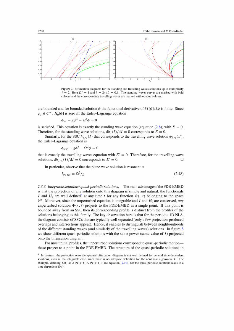
Figure 7. Bifurcation diagrams for the standing and travelling waves solutions up to multiplicityj = 2. Here �2 = 1 and k = 2π/L = 0.9. The standing waves curves are marked with boldcolours and the corresponding travelling waves are marked with opaque colours.

are bounded and for bounded solution φ the functional derivative of δI [φ]/δφ is finite. Sinceφj ∈ C∞, H ′

0[φ] is zero iff the Euler–Lagrange equation

φxx − gφ3 − �2φ = 0

is satisfied. This equation is exactly the standing wave equation (equation (2.8)) with E = 0.Therefore, for the standing wave solutions, dhj (I )/dI = 0 corresponds to E = 0.

Similarly, for the SSC hj,vk(I ) that corresponds to the travelling wave solution φj,vk

(x ′),the Euler–Lagrange equation is

φx ′x ′ − gφ3 − �2φ = 0

that is exactly the travelling waves equation with E′ = 0. Therefore, for the travelling wavesolutions, dhj,vk

(I )/dI = 0 corresponds to E′ = 0. �

In particular, observe that the plane wave solution is resonant at

Ipw-res = �2/g. (2.48)

2.3.3. Integrable solutions: quasi-periodic solutions. The main advantage of the PDE-EMBDis that the projection of any solution onto this diagram is simple and natural: the functionalsI and H0 are well defined6 at any time t for any function �(·, t) belonging to the spaceH1. Moreover, since the unperturbed equation is integrable and I and H0 are conserved, anyunperturbed solution �(x, t) projects to the PDE-EMBD as a single point. If this point isbounded away from an SSC then its corresponding profile is distinct from the profiles of thesolutions belonging to this family. The key observation here is that for the periodic 1D NLS,the diagram consists of SSCs that are typically well separated (only a few projection-producedoverlaps and intersections appear). Hence, it enables to distinguish between neighbourhoodsof the different standing waves (and similarly of the travelling waves) solutions. In figure 8we show different quasi-periodic solutions with the same power (same value of I ) projectedonto the bifurcation diagram.

For most initial profiles, the unperturbed solutions correspond to quasi-periodic motion—these project to a point in the PDE-EMBD. The structure of the quasi-periodic solutions in

6 In contrast, the projection onto the spectral bifurcation diagram is not well defined for general time-dependentsolutions, even in the integrable case, since there is no adequate definition for the nonlinear eigenvalue E. Forexample, defining E(t) as K(�(x, t))/I (�(x, t)) (see equation (2.10)) for the quasi-periodic solutions leads to atime dependent E(t).


–2.5 –2 –1.5 –1 –0.5 0 0.5 1 1.5 2 2.50

0.2

0.4

0.6

0.8

1

1.2

1.4

1.6

1.8

H0

I

A B C D

Figure 8. Solutions of the integrable equation: surface plots (right) and projections to thePDE-EMBD (H0, I ) (left). I = 0.7 for all profiles. A, B lie near the outer 1, 2 multiplicitystanding waves, C lies near the homoclinic orbit of the plane wave and D lies near the 1 multiplicityinner standing wave.

the neighbourhood of the three types of periodic standing and travelling waves families ofsolutions (the plane waves, the inner-dnoidal and the outer-cnoidal waves) is nicely organizedby the PDE-EMBD skeleton. Quasi-periodic solutions near the stable branches of these SSCsoscillate around them. Quasi-periodic solutions that are located near unstable branches shadowtheir homoclinic orbits.

Moreover, we show next that the plane wave SSC splits the integrable solutions in itsneighbourhood into two distinct families. Consider the near-plane wave family of solutions�ini-2(x, t) with two-mode initial data: �ini-2(x, 0) = �ini-2(x) = [ 1√

2|c| + (q + ip) cos(kx +

θ)]eiγ (0), where q, p ∈ R, 0 < |q| + |p| � 1, and qp = 0. Denote by |c′| the amplitude of theplane wave solution that has the same power I as �ini-2(x), and let δ2 := q2 + p2:

I = 12 |c′|2 = 1

2 (|c|2 + q2 + p2) = 12 (|c|2 + δ2). (2.49)

We call such solutions with δ � 1 ‘exterior’ if either 12 |c′|2 � I1LUM or { 1

2 |c′|2 > I1LUM

and p �= 0}, and ‘interior’ if { 12 |c′|2 > I1LUM and q �= 0} (this definition is motivated by the

structure of the truncated model, see section 3.1). We now establish:

Theorem 6. The projections of ‘exterior’ (respectively ‘interior’) solutions to the PDE-EMBDare to the left (respectively to the right) of the plane wave SSC.

Proof. Since we consider the integrable dynamics the constants of motion are preserved andhence I (�ini-2(x, t)) = I2(|c|, q, p) := 1

2 (|c|2 + q2 + p2) and similarly H0(�ini-2(x, t)) =H0,2(|c|, q, p) where

H0,2(|c|2, q, p) = −k2

2(q2 + p2) +

g

8|c|4 +

3g|c|2q2

4+

g|c|2p2

4+

3g(q2 + p2)2

16

− �2|c|22

− �2(q2 + p2)

2.

To prove the theorem, we need to show that for the exterior solutions H0,2(|c|2, q, p) <

H0(|c′|2, 0, 0) whereas for the interior solutions the opposite inequality holds. First, note that

H0,2(|c′|2, 0, 0) = g

2(I )2 − �2I = g

8|c|4 +

g|c|2δ2

4− �2|c|2

2− �2δ2

2+

g

8δ4.


Now, for the exterior orbits with p �= 0 we have

H0,2(|c|2, 0, δ) = −k2δ2

2+

g|c|2δ2

4+

g

8|c|4 − �2|c|2

2− �2δ2

2+

3gδ4

16

= H0,2(|c′|2, 0, 0) − k2δ2

2+

gδ4

16< H0,2(|c′|2, 0, 0),

where the last inequality holds for sufficiently small δ (δ2 < (8k2/g)), so the theorem isestablished for such solutions. The exterior orbits with q �= 0 also satisfy, by definition,12 |c|2 + 1

2δ2 � (k2/2g) = I1LUM and thus

H0,2(|c|2, δ, 0) = −k2δ2

2+

3g|c|2δ2

4+

g

8|c|4 − �2|c|2

2− �2δ2

2+

3gδ4

16

= H0,2(|c′|2, 0, 0) + δ2

(−k2

2+

g|c|22

)+

gδ4

16

� H0,2(|c′|2, 0, 0) − 7gδ4

16< H0,2(|c′|2, 0, 0),

as claimed. Finally, this last inequality is reversed for interior orbits; Indeed, the above calcu-lation shows that H0,2(|c|2, δ, 0) > H0,2(|c′|2, 0, 0) provided δ2 > (16/g)((k2/2)−(g|c|2/2)).Utilizing the definition of c′ (equation (2.49)) we obtain that this inequality is satisfied whenδ2 < 16

7 ((|c′|2/2) − (k2/2g)), namely that for (|c′|2/2) > I1LUM and sufficiently small δ thereverse inequality indeed holds. �

3. The near-integrable dynamics

Consider now the perturbed NLS equation, namely equation (1.2). In the autonomous frame(� = ϕei�2t−iα) the equation becomes

i�t − �xx − (g|�|2 − �2)� = ε − iδ�, (3.1)

where ε is the forcing amplitude, δ is the damping coefficient and ε, δ � 1. We will mostlyconcentrate here on the forced (undamped) equation (δ = 0, ε �= 0). This equation isconservative, as the total Hamiltonian

HT (�) = H0(�) + εH1(�), H1(�) = 1

L

∫(�∗ + �) dx (3.2)

is preserved (whereas the damping term dissipates the energy).The forced system is chaotic and exhibits rich behaviour. Since there is no dissipation of

energy, regular, temporal chaotic and spatio-temporal chaotic solutions co-exist. We proposethat there are three useful projections of the solutions that are helpful in distinguishing betweendistinct solutions: projections onto the PDE-EMBD, the phase–power projection and the qp

projection. These projections are motivated by the study of a two-mode truncation of theforced NLS, a model that turned out to contribute much to our understanding of the evolutionof solutions with the initial nearly flat low-amplitude profile [51, 52]. We thus review nextthe construction of the two-mode model and explain what are the phase–power and the qp

projections. We then use these projections to explain the phase-space structure of the perturbedPDE dynamics near the plane waves, demonstrating that the projections allow us to distinguishbetween various types of solutions. We end this section by analysing one of the recentlydiscovered chaotic solutions—the parabolic resonant type: we show that the truncated modelmay be used to predict the extent of the instabilities associated with this solution.


3.1. The two degrees of freedom model

The two degrees of freedom (d.o.f) truncated model of the forced NLS was proposedin [10, 12, 38] as a simplified phenomenological model to characterize some of the observednear-integrable dynamics of the NLS PDE and was studied in [31, 38, 51]. The model is derivedby substituting in the forced NLS the finite expansion7,

�N+1(x, t) = 1√2|c(t)|eiγ (t) + b(t)eiγ (t) cos(kx) + a1(t)e

iγ (t) sin(kx)

+N∑

n=2

(an(t)eiγ (t) sin(knx) + bn(t)e

iγ (t) cos(knx)),

truncating the equations at N = 1, and considering only symmetric initial profiles (settinga1(t) = 0), see [32, 38, 51]. While there is not yet a rigorous justification for this crudetruncation, it appears to provide a fairly accurate description of the PDE dynamics nearthe plane waves as long as I , the L2 norm of the solution, satisfies I < I2LUM [10–12, 17, 52]. Indeed, near the plane wave, linear stability (equation (2.40)) shows thatthe higher modes cos (nkx), sin(nkx), n = 2, .., ∞ are stable with frequency ωn =√

(2πn/L)4 − 2g(2πn/L)2|c|2 = O(n2), and thus, in the non-resonant case, can be treatedas stable oscillators. Since these modes are much faster than the first and the second modes(the frequency increases as n2), one expects that resonances will be rear and that the slowdynamics will essentially decouple from the fast modes (see [22, 26] for related results). Theresulting truncated system is a near-integrable two d.o.f Hamiltonian of the form H (b, c) =H0(b, c) + εH1(b, c), where, in the integrable limit (ε = 0), I = 1

2 (|c|2 + |b|2) = ||�2(x)||L2

is preserved.

3.1.1. The integrable system. The first main step in the analysis of the truncated integrabledynamics (ε = 0) is a transformation from the Fourier mode amplitudes (c, b) to the generalizedaction-angle coordinates (q, p, I , γ ) [38]:

c = |c| exp(iγ ), b = (q + ip) exp(iγ ), (3.3)

I = 12 (|c|2 + q2 + p2). (3.4)

The transformation brings the Hamiltonian H0(b, c) to the form

H0(q, p, I ; �2, k2, g) = g

2(I )2 − �2I +

(gI − 1

2k2

)q2 − 7g

16q4 − 3g

8q2p2

+g

16p4 − 1

2k2p2,

where

(I , γ ) ∈ (R+ × T ), (q, p) ∈ BI = {(q, p)|q2 + p2 < 2I }and the truncated model depends on the two parameters �2 and k = 2π/L. The two truncatedintegrals of motion H0 and I are analogous to H0 and I of the PDE.

Once these coordinates are introduced8, the structure of the unperturbed solutions and thestructure of the unperturbed energy surfaces may be easily found. Since I is a constant ofmotion and H0 is independent of γ , for any given I (0) the Hamiltonian H0(q, p, I (0)) may beviewed as a one-degree of freedom Hamiltonian (we refer to it as the reduced Hamiltonian) that

7 Here c(t), b(t), bn(t), an(t) are complex functions and γ (t) is the phase of c(t).8 Notice though that, as opposed to regular action-angle coordinates, the velocity of γ along the unperturbed quasi-periodic trajectories is usually non-constant.


Figure 9. The structure of the two d.o.f model (k = 1, �2 = 1, g = 2). (a) The EMBD: the greyarea denotes the allowed region of motion, the coloured curves denote the families of the singularcircles. (b) The (q, p) phase plane at I = 0.75 (the horizontal line in the EMBD). The projectionsof perturbed regular interior (magenta) and regular exterior (black) solutions onto the EMBD andonto the qp plane are shown.

controls the motion in the (q, p) plane, namely, the motion occurs along the closed qp-level9

sets of H0(q, p, I ). The topology of the level sets of the truncated two d.o.f. system maybe easily found: for (q, p) ∈ BI , each qp-level set is crossed with a circle of phases γ . ForI < I1LUM, the reduced Hamiltonian has a single elliptic fixed point at the origin (correspondingto the plane wave solution and denoted by (q

pwf , p

pwf ) = (0, 0)) and all the other qp-level sets

of H0(q, p, I ) are regular and diffeomorphic to circles that encircle it. Thus for I < I1LUM,the level sets of the two d.o.f. system correspond to a single torus, with only two exceptions ofsingular level sets that correspond to a circle: the qp origin multiplied by a circle of phases γ

and the boundary of BI (namely, the circle q2 +p2 = 2I , where c(t) = 0 and γ is not defined).At I1LUM the origin undergoes a pitchfork bifurcation, so that for I ∈ (I1LUM, I2LUM) the

reduced Hamiltonian has a figure eight structure (see figure 9(b)). The regular level sets of thetwo d.o.f. system correspond to either a single torus (for exterior qp-orbits, namely orbits inthe qp plane that encircle the figure eight) or to two disconnected tori (for interior qp-orbits,one in each of the figure eight loops, see figure 9(b). These qp plots motivated the PDEdefinition of interior and exterior orbits that appear in theorem 6. For these values of I thereare four singular level sets: the circle corresponding to the boundary of BI , the two circlescorresponding to the elliptic points inside the figure eight, and the two-dimensional level setthat corresponds to a circle in γ crossed with the qp-figure eight.

The above description provides a full characterization of the level sets of the Hamiltonianfor any fixed I < I2LUM. To obtain from it the structure of the energy surfaces, which isinstrumental for providing a qualitative prediction of the perturbed dynamics as explainednext, we construct the energy–momentum bifurcation diagram (EMBD) [7, 20, 39, 40, 51, 54].In this bifurcation diagram we plot, in the plane of (H0, I ), the singular curves—the curvesthat correspond to the singular level sets. Namely, we plot hs(I ) = (H0(qf (I ), pf (I ), I ), I ),where (qf (I ), pf (I )) stand for either one of the three fixed points in the (q, p) plane or to theboundary of BI . The region of allowed motion is the region bounded between the stable curvesin the EMBD (grey region in figure 9(a)). Every point that belongs to the allowed region ofmotion corresponds to a single level set, which may have either one or two components. Theenergy surface H0(q, p, I , γ ; �2, k2, g) = h corresponds to the intersection of a vertical lineH0 = h with the grey region in this diagram.

9 i.e. the level set of H0(q, p, I (0)) in the (q, p) plane.


Points along this energy surface line that do not belong to the singular curves correspondto regular level sets. The motion on these level sets is generically quasi-periodic, yet thereare dense set of points on which the motion is resonant (namely, there exist n, m ∈ Z with|n| + |m| �= 0, so that the two frequencies that arise obey nw1 + mω2 = 0). Similarly, themotion on the singular level sets, which are composed of circles, is called resonant if the normalfrequency (the imaginary eigenvalues of the linearized reduced Hamiltonian at the qp-fixedpoints) and the frequency of the motion along the circle (γ |{qf ,pf,I }) are resonant. The strongest

resonant circle10 thus appears when γ |{qf ,pf ,I res} = 0. Then, (qf , pf , I res, γ ) is a circle of fixedpoints (see [38, 51]). In fact, such a circle of fixed points always corresponds to an extremumof the singular curves, namely dhs(I )/dI = 0 exactly at such a resonant circle (and thereforethe foliation of the energy surface changes at such points, see [48, 51]). For the plane wavesolution, such a circle of fixed points appears at

I res = �2

g, (3.5)

the same power at which the PDE plane wave is resonant, see equation (2.48).Finally, note that the singular plane wave curve (hpw

s (I ) = (H0(0, 0, I ), I )) splits theneighbourhood of the plane wave into two distinct regions: to the right of the plane wave thequasi-periodic solutions follow the ‘interior’ part of the homoclinic solution in the (q, p) planeand each level set is composed of two-tori. The solutions to the left of the plane wave curvefollow the ‘exterior’ part of the homoclinic orbit and the level set corresponds to a single torus.Theorem 6 shows that provided the initial profile has all of its power in the first two modes(so �(x, 0) = �ini-2(x)), the PDE-EMBD inherits this property as well (similar property isexpected to hold for initial data with sufficiently rapid decay of higher modes).

3.1.2. The near-integrable system. Now consider the perturbed truncated system:

H (q, p, I , γ ) = H0(q, p, I ) + εH1(q, p, I , γ ), (3.6)

where

H1(q, p, I , γ ) =√

2√

2I − q2 − p2 sin γ. (3.7)

The solution structure of the resulting two d.o.f near-integrable system depends on theparameters (L, �; g), the energy level, and the phase-space region (we consider here only thePDE relevant region, I � I2LUM) and are roughly divided into regular and chaotic solutions.

Regular solutions. In the limit of small ε, by the KAM theorem, most initial conditionsevolve as quasi-periodic solutions. We call such solutions regular solutions. The regularquasi-periodic solutions are either ε-close to some unperturbed solutions (the non-resonantcase) or may correspond to quasi-periodic motion surrounding resonant periodic solutionswith I variations of order

√ε (KAM tori of the partially averaged system near resonances).

These solutions appear for typical initial data (qi, pi, Ii , γi) belonging to the regions of theEMBD that are at least ε away from the unstable part of the singular plane wave curve (i.e. forall Ii ∈ (I1LUM, I2LUM), we take |H0(qi, pi, Ii) − h

pws (Ii)| > O(ε)):

Non-resonant elliptic solutions. The EMBD region to the left of the plane wave curve hpws (I )

at small I values (I < I1LUM), corresponds, in the unperturbed case, to elliptic orbits: qp orbitsthat encircle the origin and appear as horizontal lines in the (γ, I ) plane. The non-resonantperturbed trajectories follow ε-closely such integrable trajectories in both (q, p) and (γ, I )

10 The smaller is |n| + |m|, the stronger is the resonance.


planes. On the EMBD, such perturbed solutions cover, in a regular pattern, a square of widthO(ε) to the left of the plane wave curve.

Non-resonant exterior solutions. The EMBD region to the left of the plane wave curve hpws (I )

with I in the unstable regime (I1LUM < I < I2LUM), corresponds, in the unperturbed case, toexterior orbits: qp orbits that encircle the figure eight homoclinic orbit associated with I andappear as horizontal lines in the (γ, I ) plane. The typical perturbed solutions with initial datain this region (that is ε-away in H0 from h

pws (I )), follow the unperturbed dynamics exactly as

in the elliptic case, see, e.g. the outer to the homoclinic orbit (black) trajectory in figure 9(b).

Non-resonant interior solutions. The EMBD region to the right of the plane wave curve hpws (I )

with I in the unstable regime (I1LUM < I < I2LUM), corresponds, in the unperturbed case,to interior orbits: qp orbits that are inside the right or left part of the figure eight homoclinicorbit associated with I . The corresponding regular perturbed solutions (namely solutions withinitial data that project to the same region of the EMBD) follow the unperturbed dynamics,see, e.g. the interior to the homoclinic orbit (magenta) trajectory in figure 9(b).

Regular resonant solutions. When a resonance occurs at a regular level set, namely anunperturbed two torus is resonant, a resonance region of O(

√ε) is created in the (γ , I )

plane, where γ denotes the resonant phase angle. The perturbed solutions follow the levellines of the partially averaged Hamiltonian in the (γ , I ) plane (slow pendulum-like dynamics)while encircling (fast dynamics) the corresponding qp-level set. By the KAM theorem forthe partially averaged Hamiltonian, most solutions in this region are quasi-periodic, and theexceptional set is exponentially small (we disregard this exceptional set in our classification).Projecting such solutions to the EMBD produces a rectangle of H -width of O(ε) and I -heightof O(

√ε). In particular, the resonant solutions in the flat plane, where b(0) = b(t) = 0, may

be easily found; On this invariant plane:

H (0, 0, I , γ ) = g

2(I )2 − �2I + 2ε

√I sin γ, (3.8)

so the half-width of the resonance zone near I res, in which regular oscillatory motion in γ

occurs, is

�I = 2√g

√�ε√

g. (3.9)

Chaotic solutions. Solutions with typical initial data (qi, pi, Ii , γi) near the unstable branchof the plane wave exhibit chaotic behaviour. Three observable11 chaotic mechanisms associatedwith the appearance of homoclinic orbits at I � I1LUM (see figure 3 in [52] and figure 11 ofsection 3.2 for the similar PDE projections to the PDE-EMBD) appear:

Homoclinic chaos. For any given δ, for sufficiently small ε, solutions with typical initial datachosen close to the homoclinic orbits with Ii ∈ (I1LUM, I2LUM) \ [I res − δ, I res + δ] evolvechaotically in the (q, p) plane as in periodically forced one d.o.f systems. Since γ(0,0,I (t)) �= 0for such solutions, the section γ = γ0 provides a local Poincare map near the correspondinghyperbolic circle, and thus transverse intersections of the circles’ stable and unstable manifoldswith O(ε) splitting angle may be established by standard methods. Thus, we say that suchchaotic solutions are created by the standard homoclinic chaos mechanism. Away from thesingular circle the motion in γ may be non-monotone, yet, in the non-resonant cases, the

11 We disregard here the complicated behaviour which includes chaotic motion in the exponentially small regions nearresonances boundaries.


distribution of γ values along chaotic trajectories appears to be uniform (islands of stabilityin the homoclinic region may destroy this uniformity in γ ). The projection of such solutionsonto the EMBD appears as almost horizontal lines (with slope of O(ε)) that occasionally crossthe plane wave curve h

pws (I ). Eventually, the projection covers, in an irregular way, a square

of width O(ε) near the initial data projected point (H0(qi, pi, Ii , γi), Ii).

Hyperbolic resonance. Solutions with typical initial data chosen close to the homoclinic orbitof a resonant hyperbolic circle, namely, with Ii = I res + O(

√ε) exhibit chaotic behaviour

which is of essential different characters than the standard homoclinic chaos [31, 32, 38]. Notethat such solutions appear only when the resonant plane wave is unstable (I res > I1LUM),namely, when �2 > �2

PR = k2/2. Away from the q = p = 0 invariant plane, such orbitsfollow the homoclinic loop, whereas near this plane they shadow the resonant slow pendulum-like dynamics in the (γ, I ) plane. Thus, in this case the variations in I are of O(

√ε). On

the EMBD, the projection of such solutions appears as almost horizontal lines with occasionalfast O(

√ε) drops in I , covering eventually a rectangle of width O(ε) and height O(

√ε) near

(H0(qi, pi, Ii , γi), Ii).

Parabolic resonance. Near the critical parameters value �2 ≈ (k2/2) (where I res ≈ I1LUM),typical solution with initial data in the neighbourhood of the nearly parabolic and nearlyresonant plane wave exhibit intermittent chaotic behaviour. The projection of such solutionsto the EMBD appears to oscillate along the parabola-shaped lines, changing their fidelityas these lines cross the plane wave curve h

pws (I ). These projections cover eventually an arched

shape region of width O(ε) and height O(√

ε) near (H0(qi, pi, Ii , γi), Ii). Following [50],we show in section 3.3 that the parabola-like level lines correspond to an adiabatic invariantthat is preserved by the perturbed trajectories as long as they are away from the plane waveseparatrices, namely their projection is away from the curve h

pws (I ).

3.2. The perturbed PDE phase-space structure near the plane waves

The nonlinear chaotic nature of the truncated system suggests that a standard comparisonbetween perturbed and unperturbed solutions of the PDE (e.g. plotting time integral ofthe L2 norm of the difference between the solutions) will not be informative. Instead,we seek qualitative comparison between the solutions. These are achieved by comparingthe three projections that were introduced in the two d.o.f analysis, where the generalizedaction-angle coordinates (q, p, I , γ ) were naturally defined. Denote by Cn�(x, t) =�(n, t) the nth complex coefficient of the Cosine tranform of the solutions (Cn�(x, t) =1L

∫ L/2−L/2 �(x, t) cos(nkx) dx), and define the following three projections of the PDE

solutions:

(P1) Projection onto the PDE-EMBD. We plot the parametric curve {ζt }t∈[0,τ ] where ζt =(H0(�(x, t)), I (�(x, t))) (recall equations (2.2) and (2.4)) on top of the skeleton of theprojections of the unperturbed standing and travelling wave solutions. Note that by (3.2)the curve {ζt }t∈[0,τ ] always (for all τ ) projects into a strip of width O(ε) in H0 aroundthe initial energy H0(�0(x)).

(P2) Projection onto the phase–power plane. We plot the parametric curve {ρt }t∈[0,τ ] in the(γ, I ) plane, namely we plot ρt = (γ (t), I (�(x, t))). Here γ (t) = arg C0�(x, t) is thephase of the flat part of the solution.

(P3) Projection onto the (q, p) plane. We plot the parametric curve {ξt }t∈[0,τ ] in the (q, p)

plane, where (q, p) are defined as the real and imaginary parts of the first mode of thesolution (phase shifted to match the flat phase):

ξt = (Re[C1�(x, t)e−iγ (t)], Im[C1�(x, t)e−iγ (t)]). (3.10)


We show that these projections reveal, on the one hand, the analogy between the ODE andthe PDE solutions, and on the other hand, enable to detect when the PDE behaviour is distinctfrom the ODE. A few notes are in order:

1. These projections hide the explicit time dependence of the solutions, as appropriate forthe qualitative comparison between perturbed and unperturbed solutions.

2. Note that the first projection uses the integrable PDE structure as an underlying skeletonfor the motion, thus providing accurate division of the projected PDE space to interiorand exterior solutions for initial data that is located near the plane wave and has only twomodes (recall theorem 6).

3. Below, we utilize our understanding of the dynamics associated with the family of two-mode initial data:

�0(x) = �ini-2(x) =[

1√2|c| + b(0) cos(kx)

]eiγ (0). (3.11)

It appears that adding to such initial profiles higher modes that decay rapidly does notchange the qualitative statements regarding the dynamics (yet may shift the SCC curves).

4. Note that two-mode initial data, namely a flat mode and a first harmonic are necessarilysymmetric, hence, with no loss of generality, for such initial data we may take the symmetryaxis to be at x = 0, and thus the projection of such solutions to the (q, p) plane utilizingthe cosine transform C1 (centred at the origin) is natural.

5. We expect that in the two-mode zone, namely when I (t) < I2LUM and the initial datahave sufficiently fast decay of the high modes, the ODE and the PDE systems will behavesimilarly. Indeed, we demonstrate below that all the near-integrable ODE behavioursappear in the PDE as well. When solutions that are initialized in this zone leave it,possibly by two d.o.f. instability mechanisms that ramp I beyond the I2LUM threshold,other modes of the solution become active and, as explained in section 3.3, intermittentspatial–temporal chaos emerges.

Regular solutions. Solutions with initial profiles that are bounded away from the unstablebranch of the plane wave and its homoclinic orbits and satisfy I (0) < I2LUM are observedto execute, for sufficiently small ε (e.g. for ε ≈ 10−3 for the initial conditions shown infigure 10), quasi-periodic motion (up to the numerical accuracy). Note that the solutions thatappear in figure 10 are far from the quiescent solution, namely, they have a finite power. Infact, figure 10 shows KAM like solutions with I > I1LUM, demonstrating that away from theunstable branches of the special solutions, the perturbed PDE phase space may indeed havemany regular orbits. We conclude that an infinite-dimensional KAM theorem may hold hereeven for large amplitude solutions (see [22] for related rigorous results in the small amplituderegime).The projection ζt of such regular non-resonant orbits (respectively, resonant) to thePDE-EMBDs appears as an ordered covering of a confined rectangular region of width O(ε)

and height O(ε) (respectively O(√

ε)).The projection of the non-resonant regular perturbed solution onto the phase–power plane

appears as a band of height O(ε) around I (�0(x)) that covers uniformly all values of γ (yetγ (t) may be non-monotone), similar to the corresponding unperturbed trajectories. Resonantregular quasi-periodic motion projects to the phase–power plane as a band of height O(

√ε)

that is distinct from the projection of the integrable solutions, and, in particular it is non-uniform in γ . The projection to the qp-plane of both the unperturbed and perturbed solutionsis non-trivial as the true second mode is composed of many Fourier components. Nonetheless,it provides information regarding exterior and interior type of dynamics.


(a) (b)

(c)

–0.8 –0.6 –0.4 –0.2 0 0.2 0.4 0.6 0.80

0.1

0.2

0.3

0.4

0.5

0.6

0.7

0.8

0.9

1

H0

I

–0.5 –0.3 –0.1 0.1 0.3 0.5–0.5

–0.3

–0.1

0.1

0.3

0.5

q

p

–1 –0.5 0 0.5 1

–1

–0.5

0

0.5

1

q

p

Figure 10. Three perturbed regular PDE solutions. The magenta/black/cyan orbits are the P1(a) and P3 (b), (c) projections of the near-integrable regular interior/exterior/elliptic solutions(with ε = 10−3, k = 1, �2 = 1, g = 2). Some of the integrable solutions (blue—theplane wave and its homoclinic orbits, green—the inner solution with multiplicity 1, red—theouter solutions) are shown. (a) The PDE-EMBD for I < I2LUM, with the three P1 projectionsof the solutions. (b) P3-projection (to the qp-plane) of an elliptic solution with initial data

�0(x) = [√

0.1√2

+√

0.1 cos(kx)]eiγ (0) (so I (t = 0) = 0.15). The origin (blue point) is

the P3-projection of the stable plane wave at I = 0.15. (c) P3-projection of the exterior

(�0(x) = [√

1.1√2

|c| +√

0.4i cos(kx)]eiγ (0)) and interior (�0(x) = [√

0.9√2

|c| − √0.6 cos(kx)]eiγ (0))

solutions at I (t = 0) = 0.75 (the horizontal line in the PDE-EMBD). The dashed blue curves(respectively green points) are the P3-projections of the symmetric unperturbed homoclinic orbitsto the plane wave (of the symmetric unperturbed inner-dnoidal solutions with multiplicity 1).

We can now classify the typical PDE quasi-periodic motion near the plane waves to fourclasses of solutions that are similar to the ODE classes. Yet, the classification here is non-rigorous (in particular, note that in the ODE case each point on the EMBD corresponds toa unique level set of the integrable motion, whereas the PDE-EMBD does not preserve thisproperty). Thus, we present numerical evidence for its validity for the two-mode initial data ofthe form (3.11) that was considered in theorem 6. We emphasize that here only the initial dataare taken in the truncated form—the forced NLS equations are integrated with an 8th orderfinite-difference in space and 4th order Runge–Kutta in time scheme (similar results appearwhen a spectral code with 512 modes is utilized), and for all t > 0 we do observe that somesmall power is spread to the higher Fourier modes.

Non-resonant elliptic solutions. Solutions with initial profiles (3.11) satisfying I (�0(x)) <

I1LUM are typically, for sufficiently small ε, quasi-periodic and remain ε-close to a nearbyintegrable solution. Their projection to the PDE-EMBD lies to the left of the plane wave SSC


curve (see figure 10(a) and theorem 6). Their projection to the qp-plane, ξt , results with orbitsencircling the origin, see figure 10(b). Their projection ρt onto the phase–power plane appearsas ε-deformed horizontal lines (not shown).

Non-resonant exterior solutions. Similarly, for most initial profiles of the form (3.11) satisfyingRe[b(0)] = 0, Im[b(0)] �= 0 and I (�0(x)) ∈ (I1LUM, I2LUM), the perturbed solutions arequasi-periodic and remain ε-close to an exterior integrable solution oscillating around theouter-cnoidal like solutions (figure 10(c)). Their projection onto the PDE-EMBD is to the leftof the plane wave SSC, see figure 10(a) and theorem 6.

Non-resonant interior solutions. Solutions with initial profiles of the form (3.11) satisfyingRe[b(0)] �= 0, Im[b(0)] = 0 and I (�0(x)) ∈ (I1LUM, I2LUM) are typically quasi-periodicand remain ε-close to an integrable solution which oscillates about the inner-dnoidal standingwave in the interior of the homoclinic orbit, see figure 10(c). The sign of Re[b(0)] determineswhether the solution oscillated about the right (Re[b(0)] > 0) or left (Re[b(0)] < 0) dnoidalstanding wave. In contrast to the two d.o.f case, the projected interior integrable orbits to theqp-plane may have a complicated shape, see figure 10(c). The projection of such perturbedsolutions onto the PDE-EMBD is to the right of the plane wave SSC, see figure 10(a) andtheorem 6.

Resonant solutions. Resonant elliptic, interior and exterior solutions appear for a ‘smallfraction’ of the above listed initial profiles12. Their projections onto the PDE-EMBD andthe qp-plane, extends to variation of O(

√ε) in I . Their projection to the (γ, I ) plane, in

the rotational resonant frame, is pendulum-like. The strongest resonances, namely thosethat appear at the folds of the different SSC in the PDE-EMBD (theorem 5), produce thelargest resonance zones. In particular, if �2 < �2

PR, then the plane wave SSC has a fold atIpw-res < I1LUM and thus, for most initial profiles �0(x) in the rectangle of height O(

√ε) near

this fold (with ε sufficiently small so that√

ε � (I1LUM − Ipw-res)) the perturbed solutions areresonant yet regular. Their projection onto the phase–power plane is pendulum-like and theseare easily observable even for ε ≈ 10−3. See figure 1(a) in [53] for such trajectories in thecase of relatively large ε, where the resonant zone exceeds the I1LUM bound.

Temporally chaotic solutions. Perturbed solutions that visit the neighbourhood of the planewave in its unstable regime (I ∈ (I1LUM, I2LUM)) yet do not invade the region I > I2LUM

exhibit temporal chaos that follow closely the two d.o.f orbits. As in the two d.o.f. case,three observable chaotic scenarios arise, and their projections P1–P3 to the three planes—thePDE-EMBD, the (γ, I ) plane and the (q, p) plane follow closely those of the ODE;

Homoclinic chaos. Given a δ > 0, for sufficiently small ε, solutions with initial profiles ofthe form (3.11) satisfying 0 < |b(0)| = O(ε) and I (�0(x)) ∈ (I1LUM, I2LUM) \ [Ipw-res −δ, Ipw-res + δ], will typically exhibits homoclinic chaos. Such initial profiles project onto thePDE-EMBD in an O(ε) neighbourhood of the SSC in the interior of the interval (I1LUM, I2LUM),at a point which is bounded away from the resonant plane wave solution, the SSC extremapoint Ipw-res = �2/g (= 0.4 in figure 11(HC)). The projected curve is composed of nearlyhorizontal lines (corresponding to the homoclinic excursions along which I changes by O(ε))and occasional crossing of the SSC curve (see figure 11).

Hyperbolic resonance. For �2 ∈ (k2/2, 2k2), for sufficiently small ε, solutionswith initial profiles of the form (3.11) satisfying 0 < |b(0)| = O(ε) and

12 The initial profile (3.11) depends on four real parameters, {|c|, γ (0), Re[b(0)], Im[b(0)}, and since we takeI < I2LUM these parameters belong to a bounded domain. Thus the notion of typical initial condition of thisfamily may be precisely defined.


–0.15 –0.148 –0.146

0.49

0.5

0.52

0.53

H0

I

–0.1605 –0.1595 –0.1585 –0.157

0.385

0.39

0.4

0.405

H0

I

–0.0435 –0.0425 –0.0415

0.15

0.17

0.19

0.21

H0

I

Figure 11. Three different types of temporal chaos in the forced NLS equation. The periodiclength is fixed to k = 2π/L = 0.9 and the initial profile is near the unstable plane wave:�0 = √

Aeiγ0 + 10−5 cos kx, ε = 10−3, with the values (HC) Homoclinic chaos: �2 = 0.8, A =0.5, γ0 = 1/4π (HR) Hyperbolic resonance: �2 = 0.8, A = 0.4, γ0 = 1/4π and (PR) Parabolicresonance: �2 = 0.405, A = 0.2, γ0 = 3/4π .

I (�0(x)) ∈ [Ipw-res − O(√

ε), Ipw-res + O(√

ε)], typically exhibit hyperbolic resonance chaos.The initial profile projects onto the PDE-EMBD in a rectangle of height O(

√ε) that

crosses the SSC in the interior of the interval (I1LUM, I2LUM) near the SSC extremal pointIpw-res, see figure 11(HR). The projected curve is composed, as in the truncated case, fromalmost horizontal lines (homoclinic excursions) and abrupt O(

√ε) excursions in I that

correspond to some shadowing of the resonance zone dynamics (see [32, 38] for relatedanalysis).

Parabolic resonance. Near the critical parameters’ values �2 ≈ �2PR = (k2/2) (where

Ipw-res ≈ I1LUM), for sufficiently small ε, solutions with initial profiles of the form (3.11)satisfying 0 < |b(0)| = O(ε) and I (�0(x)) ∈ [Ipw-res − O(

√ε), Ipw-res + O(

√ε)], typically

exhibit the parabolic-resonance chaos, see figure 11(PR). The shape and form of these parabolicresonant solutions are similar to that of the parabolic resonant solutions of the truncated systemas long as I (t) < I2LUM [52]. This latter condition is satisfied in the limit of sufficiently smallε. In section 3.3 we show that these solutions actually follow the level lines of an adiabaticinvariant of a simplified two d.o.f. normal form, thus finding the scaling for the observedintermittent chaotic motion.

Spatio-temporal chaotic solutions. When solutions are either initialized or evolve to theregion near the plane wave with I > I2LUM, spatio-temporal dynamics arise. Then, at leasttwo spatially non-trivial modes evolve chaotically in time, typically with chaotic relativephase, and thus their spatial profile becomes uncorrelated [18, 53]. Since the perturbedsystem preserves the space of spatially symmetric functions (see [17]), such a behaviouris possible only when asymmetric initial data are introduced (yet, we find that even theslightest asymmetry in the initial data or in the numerical code is sufficient to induce theappearance of STC when I (t) > I2LUM). We can thus conclude that if a typical (asymmetric)solution projection to the PDE-EMBD crosses the I = I2LUM line near the plane wave SSC,


it exhibits STC13. Auto-correlation plots, amplitude plots or even Fourier mode phase plotssupport this observation [53]. Can a nearly quiescent initial profile (with small I (0)) evolveto reach the temporal-chaos region (with I (t) > I1LUM) or even the spatial–temporal region(I (t) > I2LUM)? We propose that for sufficiently small ε the answer is negative: the numericalindications are that for small ε the nearly quiescent solutions of the forced NLS behave asthe solutions of the truncated model, where, by KAM theory, they cannot increase their initialpower by more than O(

√ε) and thus remain forever in the small I region (for the forced

NLS—these are finite-time numerical results).On the other hand, for sufficiently large ε it is always possible to ramp I up to I2LUM on a timescale of order O(1/

√ε) by the plane wave resonance mechanism; Indeed, note that on this

flat invariant plane the dynamics is governed by the Hamiltonian (3.8). Indeed, equation (3.9)implies that when �I � I res nearly quiescent solutions are swept into the resonances zone.Hence, for any given �, there is a critical ε0(�):

ε0(�) = �3

4√

g(3.12)

beyond which the resonance zone extends from the origin to I res+�I . Similarly, this resonancezone extends beyond I2LUM when I res + �I � I2LUM, and another critical value, ε2LUM(�, k),emerges:

ε2LUM(�, k) = 1

�√

g

(k2 − �2

2

)2

. (3.13)

Thus, for ε > εc-flat(�, k) = max {ε0(�), ε2LUM(�, k)}, the L2 norm of typical nearlyquiescent flat solutions is ramped up beyond I2LUM. Note that εc-flat(�, k) is minimal at�2 = k2. For example, for the parameters (g, k) that are chosen in [53], k = 0.9 and g = 2,εc-flat(0.9, 0.9) = (0.9)3

4√

2≈ 0.129. Non-flat nearly quiescent initial data evolve to STC when

ε > εc(�, k), where clearly εc(�, k) � εc-flat(�, k). In [53] we find numerically that εc(�, k)

is actually minimal at parabolic resonance (namely the minimum shifts to �2 = k2/2) andthat εc(

0.9√2, 0.9) ≈ 0.05.

3.3. The parabolic-resonance phenomena

The appearance of parabolic resonance in the truncated two d.o.f system (equation (3.6))may be fully analysed by transforming the truncated model into the symmetric parabolic-resonance normal form that has recently been constructed and analysed [50]. We provide thetransformation to the normal form below and show that for small ε the projection of the PDEsolution onto the first two Fourier modes (projections P2, P3 to (xp(t), yp(t), Ip(t), γ p(t)))

follow the same adiabatic invariants as the two d.o.f model.To analyse the truncated system, we introduce below a change of coordinates that brings

the truncated model, in the leading order term, to the parabolic-resonance slow-fast normalform:

H (q, p, I , γ ; g, k, �2, ε) → εnf [H nf(qnf , pnf , I nf , ϕnf; β, λ)

+ (εnf)12 Hp(qnf , pnf , I nf , ϕnf; εnf)],

13 So far, there is no indication that such solutions may lead to weak turbulence: it appears that even-though thedynamics are chaotic and involve several modes, the energy remains concentrated only in the lowest Fourier modes(see [18, 53] and figures therein).


where (hereafter we drop the nf superscripts when unambiguous)

H nf(q, p, I, ϕ) = p2

2− I

q2

2+

q4

4+ β

(λ + I )2

2+ cos ϕ (3.14)

is equipped with the slow-fast symplectic form dq ∧ dp + ε−1/4(dϕ ∧ dI ) so that thevelocities in the fast (q, p) variables are of O(1) and those in the slow (I, ϕ) variables are ofO(ε1/4).Most importantly, the parameters λ, β, ε that appear in the normal form are

λ = 128

49√

εnf

(1

2− �2

k2

), β = − 7

16, εnf = 45√2g

73k3ε ≈ 4.22

√g

k3ε (3.15)

Note, in particular, that β is independent of the forced NLS parameters, that λ is tunable bychanging � and that εnf has non-trivial dependence on k.The transformation to the normal form is given by (with a = (

√7k/4

√g), b = 2(

√7

4 )3 k√g

):

q = a4√

εnfqnf , p = b√

εnfpnf , I = ab√

εnfI nf +1

2gk2, γ = ϕnf − π/2

H = −k2b2εnfH nf − �4

2g, t = − tnf

4√

εnfk2b2.

So that the perturbation near the parabolic-resonance region becomes√

εnfHp(qnf , pnf , I nf , ϕnf; εnf) =√

εnf3

8

7

16(qnf)2(pnf)2 − εnf 73

47(pnf)4

+

(√1 +

7

16

√εnf

(7

4I nf − (qnf)2

)− εnf

73

45(pnf)2 − 1

)cos ϕ

=√

εnf

(3

8

7

16(qnf)2(pnf)2 +

7

32

(7

4I nf − (qnf)2

)cos ϕ

)+ O(εnf).

Note that for any fixed (I, ϕ) the Hamiltonian H nf(q, p, I, ϕ; β, λ) corresponds to theclassical Duffing oscillator; for negative I this Hamiltonian has a single stable fixed point atthe origin, whereas for positive I the system has a figure eight separatrix emanating from theorigin with two elliptic fixed points at (q, p) = (±√

I , 0). The motion in the (q, p) plane isfast as long as the qp orbit is bounded away from the separatrix. Thus, on each energy surfaceH nf(·) = h, we define the separatrix set Sqp(h) as the set of (I, ϕ) values that correspond tothe (q, p) separatrix level set

Sqp(h) ={(I, ϕ)|I > 0 and h = H nf(0, 0, I, ϕ) = β

(λ + I )2

2+ cos ϕ

}. (3.16)

It follows that for values of (I, ϕ) that are bounded away from Sqp(h) the motion in the (q, p)

plane is fast, and hence, by the adiabatic theorem, it preserves an adiabatic invariant [50]. Tofirst order in ε1/4, the adiabatic invariant is given by the qp-area that is enclosed by the fasttrajectories, namely the action J (I, ϕ; h):

J (I, ϕ; h) = 2∫ q+

q−p dq = 2

√2

∫ q+

q−

√z(ϕ; h) +

q2

2I − q4

4− β

(λ + I )2

2dq, (3.17)

z(ϕ; h) = h − cos ϕ, (3.18)

where q+ and q− are properly defined to make J (I, ϕ; h) continuous across the separatrix set.The perturbed motion projected to the (I, ϕ) plane follows the level lines of J (I, ϕ; h) up to


ODE-1 ODE-2 PDE

0 1 2 3 4 5 6–3

–2.5

–2

–1.5

–1

–0.5

0

0.5

1

1.5

2

φ

Inf

0 1 2 3 4 5 6–3

–2.5

–2

–1.5

–1

–0.5

0

0.5

1

1.5

2

φ

Inf

0 1 2 3 4 5 6–3

–2.5

–2

–1.5

–1

–0.5

0

0.5

1

1.5

2

φ

Inf

–1 –0.5 0 0.5 1 1.5 2 2.5–3

–2.5

–2

–1.5

–1

–0.5

0

0.5

1

1.5

2

z

Inf

–1 –0.5 0 0.5 1 1.5 2 2.5–3

–2.5

–2

–1.5

–1

–0.5

0

0.5

1

1.5

2

z

Inf

–1 –0.5 0 0.5 1 1.5 2 2.5–3

–2.5

–2

–1.5

–1

–0.5

0

0.5

1

1.5

2

z

Inf

Figure 12. Adiabatic chaos in the forced NLS. Trajectories of the forced truncated model equation(ODE-1, ODE-2 columns) and of the forced NLS PDE (PDE column) with initial conditions nearthe plane wave solution are projected (red) on top of the level sets of the adiabatic invariant of the

normal form J (I, ϕ; h). The sets corresponding to the stable plane wave (Sqp

∣∣∣{Inf <0,(q,p)=(0,0)})

and ground state (Sqp

∣∣∣{Inf >0,(q,p)=(±√

Inf ,0)}) circles and are marked by solid blue and green curves,

respectively, and the separatrix set (Sqp

∣∣∣{Inf >0,(q,p)=(0,0)}) is indicated by a dashed blue curve. First

row: the trajectories are projected to the (ϕnf , I nf ) plane. Second row: the trajectories are projectedto the (z, I nf ) plane. The vertical lines show the energy surface boundaries. In all figures h = 0.695,ε = 10−3. The initial conditions for ODE-1 and PDE are: (q, p, I, ϕ) = (10−5, 0, 0.2, 5

4 π), for

ODE-2 the initial conditions are (x, y, I, ϕ) = (5 × 10−5, 0, 0.2, 54 π).

the separatrix set, where it undergoes a jump. This quasi-regular behaviour is called adiabaticchaos: such a behaviour has been extensively studied theoretically and in the context of variousapplications [7, 19, 27, 46, 47, 56].

The level lines of J (I, ϕ; h) change their shape and even their topology for different ener-gies, thus a full description of the dynamics for all energies appears to be formidable. However,since J (I, ϕ; h) = J (z(ϕ; h), I ) and since the dependence of z on ϕ and h is so simple todecipher (see equation (3.18)), projecting the J level lines to the (z, I ) plane provides a fulldescription of the perturbed dynamics at any energy level; Up to the

√εHp corrections, the

perturbed motion at the energy level h is confined to the strip z ∈ [h−1, h+1], and thus occursalong the J level lines in that strip. The separatrix set projection to the (z, I ) plane is simplythe upper part of the parabola β((λ + I )2/2) (see equation (3.16)). Hence, at any energy, theJ level lines that intersect the separatrix set in the strip z ∈ [h − 1, h + 1] correspond exactlyto the chaotic set.

In figure 12 trajectories of the forced truncated model equation (marked as ODE-1, ODE-2)and of the forced NLS (marked as PDE) transformed to the normal form coordinate systemare shown. These trajectories (red) are compared with the level sets of the adiabatic invariantJ (I, ϕ; h) (grey) of the normal form system in the (I, ϕ) plane (first row) and in the (z, I )

plane (second row). It is clearly observed that both the PDE and the ODE perturbed trajectories


follow the level sets of the adiabatic invariant except near the separatrix set (dashed blue line).In the second row of figure 12 the trajectories are projected to the (z, I ) plane, where theenergy surface bounds on z are shown. We observe numerically that the adiabatic invariant ispreserved away from the separatrices for εnf � 0.001. For such values, the region of chaoticbehaviour is of order

√εnf , and thus, in particular the instability in I values is limited to

O(√

εnf). Notably, for k = 0.9, g = 2 we get εnf = 8.19ε. The critical value of εc = 0.05that was found numerically to produce the transition of nearly quiescent initial data to STCsolutions in [53] corresponds to εnf = 0.41, where the leading order adiabatic chaos analysisis clearly invalid.

4. Conclusions and discussion

By constructing the PDE-EMBD, we show that the standing and the travelling waves solutionsof the periodic one-dimensional NLS equation may serve as organizing skeleton for the PDEphase-space structure near these special solutions. We find that these families of solutionsproject as distinct curves (called SSC) in the PDE-EMBD. We proved that the folds of thesecurves correspond to resonances of the standing/travelling waves solutions. We completed thePDE-EMBD by including the information regarding the stability of the three families of thestanding waves. We provided a modified proof for the linear instability of the inner standingwaves solutions with multiplicity j � 2. We studied the linear stability of the outer standingwaves solutions numerically and found that these waves undergo a sequence of Hamiltonian–Hopf bifurcations. The Hopf bifurcations appear at Im

bif(�outj (x)) = (m2/g)k2, with similar

scaling to that of the plane wave modulation instability. A proof of this numerical result shouldcomplete the rigorous study of linear stability/instability of all the standing waves solutions inthe one-dimensional periodic NLS. The stability analysis of the travelling wave solutions isstill open.

The PDE-EMBD provides a convenient way to classify the solutions of the perturbedproblem near the SSCs. In an O(ε)-neighbourhood of unstable branches of the SSC, oneexpects to find chaotic solutions, whereas away from such branches, infinite-dimensionalKAM type solutions are expected to arise. Near folds of the SSC resonances are created. Weuse these observations to classify the type of solutions that appear near the plane wave, thusproviding a phase-space analysis for the PDE in the SSC neighbourhood.

For a stable KAM like solution, all constants of motion must remain in an O(ε)

neighbourhood of their initial value, and thus it projects to an ε-square in the PDE-EMBDthat is typically bounded away from any unstable SSC, see figure 10. Notably, such a solutionmust be bounded away from all other families of degenerate unstable solutions of the integrableNLS. While the PDE-EMBD that includes both the standing and the travelling waves of manymultiplicities is already rather complicated to grasp (figure 7), the full diagram should includethe bifurcating modes from the Hamiltonian–Hopf bifurcations and other finite-dimensionalquasi-periodic solutions of the integrable system. Gaps in such a diagram may indicate thestability region in which KAM like solutions reign.

When �2 ≈ k2/2 the plane wave solution has an amplitude at which it is both resonantand parabolic. In [51, 52] we showed that perturbed solutions that are initialized near the planewave exhibit instabilities that are similar to those arising in the truncated NLS equation. Herewe showed that the emerging parabolic-resonance mechanism in the truncated model may beanalysed by the adiabatic-chaos methodology. In particular, we showed that there exists anadiabatic invariant that is approximately preserved away from the separatrix set. We showedthat the PDE solutions also preserve the same invariant as long as their L2 norm does not


exceed 2k2/g. We observed that the transition to STC that was reported in [53] appears at ε

values for which the leading order approximation of the adiabatic invariant level lines is notfollowed. Since the PDE and the truncated model solutions exhibit similar behaviour at theseε values, we believe that higher order approximation of the adiabatic invariant may explainthis phenomena.

We have provided a phase-space description of the PDE solutions near the plane wavewhen it has a limited power. Clearly, the classification of perturbed motion for generalinitial data is far from being complete. Other chaotic mechanisms, for example, nearthe newly discovered Hopf bifurcations of the unperturbed outer solutions, are yet to bestudied.

Acknowledgments

The authors acknowledge the support of Israel Science Foundation (Grant 273/07),Minerva foundation and Russian-Israeli joint grant (MNTI-RFBR No 06-01-72023). Theyalso thank J Gibbon, A Soffer, E Titi, D Turaev and M Weinstein for stimulatingdiscussions.

References

[1] Ablowitz M and Segur H 1981 Solitons and the Inverse Scattering Transform (PA: SIAM)[2] Agrawal G 2001 Nonlinear Fiber Optics (New York: Academic)[3] Akhmediev N N and Ankiewicz A 1997 Solitons : nonlinear pulses and beams / Nail N. Akhmediev and Adrian

Ankiewicz (London: Chapman and Hall)[4] Pava J A, Bona J L and Scialom M 2006 Stability of cnoidal waves Adv. Diff. Eqns 11 1321–74[5] Pava J A and Natali F M A 2008 Positivity properties of the Fourier transform and the stability of periodic

traveling-wave solutions SIAM J. Math. Anal. 40 1123–51[6] Pava J A 2007 Nonlinear stability of periodic traveling wave solutions to the Schrodinger and the modified

Korteweg–de Vries equations J. Diff. Eqns 235 1–30[7] Arnol’d V I 1993 Dynamical Systems III (Encyclopedia of Mathematical Sciences vol 3) 2nd edn (Berlin:

Springer)[8] Brooke Benjamin T and Feir J E 1967 The disintegration of wave trains on deep water: I. Theory J. Fluid Mech.

Digital Arch. 27 417–30[9] Benjamin T B 1972 The stability of solitary waves Proc. R. Soc. Lond. Ser. A 328 153–83

[10] Bishop A R, Flesch R, Forest M G, McLaughlin D W and Overman II E A 1990 Correlations between chaos ina perturbed Sine-Gordon equation and a truncated model system SIAM J. Math. Anal. 21 1511–36

[11] Bishop A R, Forest M G, McLaughlin D W and Overman II E A 1986 A quasi-periodic route to chaos in anear-integrable PDE Physica D 23 293–328

[12] Bishop A R, Forest M G, McLaughlin D W and Overman II E A 1990 A modal representation of chaoticattractors for the driven, damped pendulum chain Phys. Lett. A 144 17–25

[13] Bishop A R, Fesser K, Lomdahl P S, Kerr W C, Williams M B and Trullinger S E 1983 Coherent spatial structureversus time chaos in a perturbed sine-Gordon system Phys. Rev. Lett. 50 1095–8

[14] Bishop A R and Lomdahl P S 1986 Nonlinear dynamics in driven, damped sine-Gordon systems Physica D18 54–66

[15] Bishop A, McLaughlin D W, Forest M G and Overman E II 1988 Quasi-periodic route to chaos in a near-integrablePDE: homoclinic crossings Phys. Lett. A 127 335–40

[16] Bona J 1975 On the stability theory of solitary waves Proc. R. Soc. Lond. Ser. A 344 363–74[17] Cai D, McLaughlin D W and McLaughlin K T R 2002 The nonlinear Schrodinger equation as both a PDE and

a dynamical system Handbook of Dynamical Systems vol 2 (Amsterdam: North-Holland) pp 599–675[18] Cai D, McLaughlin D W and Shatah J 1999 Spatiotemporal chaos and effective stochastic dynamics for a

near-integrable nonlinear system Phys. Lett. A 253 280–6[19] Cary J R and Skodje R T 1989 Phase change between separatrix crossings Physica D 36 287–316[20] Cushman R H and Bates L M 1997 Global Aspects of Classical Integrable Systems (Basle: Birkhauser)

http://dx.doi.org/10.1137/080718450

http://dx.doi.org/10.1016/j.jde.2007.01.003

http://dx.doi.org/10.1098/rspa.1972.0074

http://dx.doi.org/10.1137/0521083

http://dx.doi.org/10.1016/0167-2789(86)90137-5

http://dx.doi.org/10.1016/0375-9601(90)90041-L

http://dx.doi.org/10.1103/PhysRevLett.50.1095

http://dx.doi.org/10.1016/0167-2789(86)90162-4

http://dx.doi.org/10.1016/0375-9601(88)90580-4

http://dx.doi.org/10.1098/rspa.1975.0106

http://dx.doi.org/10.1016/S0375-9601(99)00057-2

http://dx.doi.org/10.1016/0167-2789(89)90086-9


[21] Davis K B, Mewes M O, Andrews M R, van Druten N J, Durfee D S, Kurn D M and Ketterle W 1995 Bose–Einstein condensation in a gas of sodium atoms Phys. Rev. Lett. 75 3969–73

[22] Eliasson L H and Kuksin S B 2010 KAM for the nonlinear Schrodinger equation Ann. Math. 172 (1) 371–435[23] Ercolani N, Forest M G and McLaughlin D W 1990 Geometry of the modulational instability: III. Homoclinic

orbits for the periodic sine-Gordon equation Physica D 43 349–84[24] Gallay T and Haragus M 2007 Orbital stability of periodic waves for the nonlinear Schrodinger equation J. Dyn.

Diff. Eqns 19 825–65[25] Gallay T and Haragus M 2007 Stability of small periodic waves for the nonlinear Schrodinger equation J. Diff.

Eqns 234 544–81[26] Geng J and You J 2005 A KAM theorem for one dimensional Schrodinger equation with periodic boundary

conditions J. Diff. Eqns 209 1–56[27] Gorelyshev I and Neishtadt A 2008 Jump in adiabatic invariant at a transition between modes of motion for

systems with impacts Nonlinearity 21 661–76[28] Grillakis M, Shatah J and Strauss W 1987 Stability theory of solitary waves in the presence of symmetry: I

J. Funct. Anal. 74 160–97[29] Grillakis M, Shatah J and Strauss W 1990 Stability theory of solitary waves in the presence of symmetry: II

J. Funct. Anal. 94 308–48[30] Grillakis M 1988 Linearized instability for nonlinear Schrodinger and Klein-Gordon equations Commun. Pure

Appl. Math. 41 747–74[31] Haller G and Wiggins S 1995 Multi-pulse jumping orbits and homoclinic trees in a modal truncation of the

damped-forced nonlinear Schrodinger equation Physica D 85 311–47[32] Haller G 1999 Chaos Near Resonance (Applied Mathematical Sciences vol 138) (Nwe York: Springer)[33] Haragus M and Kapitula T 2008 On the spectra of periodic waves for infinite-dimensional Hamiltonian systems

Physica D 237 2649–71[34] Hasegawa A 1972 Theory and computer experiment on self-trapping instability of plasma cyclotron waves Phys.

Fluids 15 870–81[35] Jackson R K and Weinstein M I 2004 Geometric analysis of bifurcation and symmetry breaking in a Gross–

Pitaevskii equation J. Stat. Phys. 116 881–905[36] Jones C K R T 1988 An instability mechanism for radially symmetric standing waves of a nonlinear Schrodinger

equation J. Diff. Eqns 71 34–62[37] Kapitula T, Kevrekidis P G and Sandstede B 2004 Counting eigenvalues via the Krein signature in infinite-

dimensional Hamiltonian systems Physica D 195 263–82[38] Kovacic G and Wiggins S 1992 Orbits homoclinic to resonances, with an application to chaos in a model of the

forced and damped sine-Gordon equation Physica D 57 185–225[39] Lerman L M and Umanskii Ia L 1994 Classification of four dimensional integrable Hamiltonian systems and

Poisson actions of r2 in extended neighborhood of simple singular points: I Russ. Acad. Sci. Sb. Math.77 511–42

[40] Lerman L M and Umanskii Ia L 1994 Classification of four dimensional integrable Hamiltonian systems andPoisson actions of r2 in extended neighborhood of simple singular points: II Russ. Acad. Sci. Sb. Math.78 479–506

[41] Magnus W and Winkler S 1966 Hill’s Equation (New York: Dover)[42] Ma Y C and Ablowitz M J 1981 The periodic cubic Schrodinger equation Stud. Appl. Math. 65 113–58[43] McLaughlin D W and Shatah J 1998 Homoclinic orbits for PDE’s Recent Advances in Partial Differential

Equations vol 54 (Providence, RI: American Mathematical Society) pp 281–99[44] Menyuk C R 1993 Soliton robustness in optical fibers J. Opt. Soc. Am. B 10 1585–91[45] Moloney J and Newell A 2004 Nonlinear Optics (Boulder, CO: Westview Press, Advanced Book Program)[46] Neishtadt A I and Vasiliev A A 1999 Change of the adiabatic invariant at a separatrix in a volume-preserving

3d system Nonlinearity 12 303–20[47] Neishtadt A 1984 The separation of motions in systems with rapidly rotating phase Prikl. Mat. Mekh. USSR

48 133–9[48] Radnovic M and Rom-Kedar V 2008 Foliations of isoenergy surfaces and singularities of curves Regular Chaotic

Dyn. 13 645–68[49] Rom-Kedar V 1997 Parabolic resonances and instabilities Chaos 7 148–58[50] Rom-Kedar V and Turaev D 2010 The symmetric parabolic resonance Nonlinearity 23 1325–51[51] Shlizerman E and Rom-Kedar V 2005 Hierarchy of bifurcations in the truncated and forced nonlinear Schrodinger

model Chaos 15 1–22[52] Shlizerman E and Rom-Kedar V 2006 Three types of chaos in the forced nonlinear Schrodinger equation Phys.

Rev. Lett. 96 024104


http://dx.doi.org/10.4007/annals.2010.172.371

http://dx.doi.org/10.1016/0167-2789(90)90142-C

http://dx.doi.org/10.1007/s10884-007-9071-4



http://dx.doi.org/10.1088/0951-7715/21/4/002

http://dx.doi.org/10.1016/0022-1236(87)90044-9

http://dx.doi.org/10.1016/0022-1236(90)90016-E

http://dx.doi.org/10.1002/cpa.3160410602

http://dx.doi.org/10.1016/0167-2789(95)00120-S

http://dx.doi.org/10.1063/1.1693996

http://dx.doi.org/10.1023/B:JOSS.0000037238.94034.75

http://dx.doi.org/10.1016/0022-0396(88)90037-X

http://dx.doi.org/10.1016/j.physd.2004.03.018

http://dx.doi.org/10.1016/0167-2789(92)90092-2

http://dx.doi.org/10.1070/SM1994v077n02ABEH003454

http://dx.doi.org/10.1070/SM1994v078n02ABEH003481

http://dx.doi.org/10.1364/JOSAB.10.001585

http://dx.doi.org/10.1088/0951-7715/12/2/010

http://dx.doi.org/10.1134/S1560354708060117

http://dx.doi.org/10.1063/1.166246

http://dx.doi.org/10.1088/0951-7715/23/6/005

http://dx.doi.org/10.1063/1.1831591



[53] Shlizerman E and Rom-Kedar V 2009 Parabolic resonance: a route to Hamiltonian spatiotemporal chaos Phys.Rev. Lett. 102 033901

[54] Smale S 1970 Topology and mechanics: I Invent. Math. 10 305–31[55] Sulem C and Sulem P-L 1999 Self-focusing and wave collapse The Nonlinear Schrodinger Equation (Applied

Mathematical Sciences vol 139) (New York: Springer)[56] Tennyson J L, John R Cary and Escande D F 1986 Change of the adiabatic invariant due to separatrix crossing

Phys. Rev. Lett. 56 2117–20[57] Weinstein M I 1985 Modulational stability of ground states of nonlinear Schrodinger equations SIAM J. Math.

Anal. 16 472–91[58] Zemlyanaya E V and Barashenkov I V 2004 Traveling solitons in the damped-driven nonlinear Schrodinger

equation SIAM J. Appl. Math. 64 800–18


http://dx.doi.org/10.1007/BF01418778


http://dx.doi.org/10.1137/0516034

http://dx.doi.org/10.1137/S0036139903424837

classification of solutions of the forced periodic nonlinear …vered/publistorder/r37_non10... ·...

Documents