Climate Engineering in an Interconnected World

- The Role of Tariffs

Markus Eigruber

Faculty of Business, Economics and Statistics

University of Vienna

Oskar-Morgenstern-Platz 1.

Phone: +43(0)1-4277-38175 | E-mail: markus.eigruber@univie.ac.at

Abstract

The goal of this paper is to investigate a plausible response to negative externalities caused by

climate engineering in a global warming context. While it is unlikely countries may directly

interfere with practices of geoengineering, one possible reaction to actions taken by others which

cause real or perceived damages in an interconnected world is given by deploying trade sanctions,

i.e. tariffs. By the means of a dynamic bilateral trade model we show that geoengineering-averse

countries have an incentive to implement/increase tariffs when climate interfering technology is

being used. We therefore argue that potential consequences on world trade patterns should not

be neglected in a comprehensive discussion about climate engineering.

Keywords: Global warming, Externalities, Tariffs, Differential game, Climate engineering.

JEL classification: Q54, Q55, Q56.

1 Introduction

The virtually unchanged reliance on the extraction and burning of fossil fuels has led to an increase of

atmospheric concentrations of CO2 from roughly 280ppm at pre-industrial times to well over 400ppm

at present. While this reliance has undoubtedly enabled modern ways of life not otherwise possible,

the benefits have been bought by future damages due to anthropogenic change in the composition of

Earth’s atmosphere and the consequent increases in temperature. Attempts to limit future damages

have been notoriously slow due to a number of different reasons. The general prisoners’ dilemma

like structure of collective vs. individual action, the issue of time discounting, large uncertainties,

1

geographic asymmetry and the global scale of the problem challenge international policy in an un-

precedented way. The recent COP21 meeting in Paris generated some optimism in form of a new

agreement, but the lack of sanction mechanisms and insufficient early contributions together with

recent experimental evidence of strategic behavior in pledge and review processes curb enthusiasm.1

Changes in attitudes towards more nationalism and protectionism in some key countries may make

it even more difficult to find a global cooperative strategy in order to optimally deal with a changing

climate in the future.

Thus, scholars have suggested alternative, technical, solutions to this problem including climate- or

geoengineering. Defined as the “...deliberate large-scale intervention in the Earth’s climate system, in

order to moderate global warming” these methods can be broadly categorized into two classes: Carbon

Dioxide Removal (CDR) and Solar Radiation Management (SRM).2 CDR methods directly remove

CO2 from the atmosphere and are generally considered to be more safe but also more expensive and act

on relatively long time-scales. No large-scale CDR technology exists today that could remove CO2 from

the atmosphere at the required rate and costs. The most promising technique of SRM, the injection of

sulphate aerosols into the stratosphere, aims at increasing Earth’s albedo - the proportion of reflected

sunlight. These aerosols increase reflectivity and therefore directly influence the Earth’s radiation

balance. It has been argued that this method could effectively and very timely lower global average

temperatures with manageable projected costs. However, many authors point out that considerable

drawbacks associated with SRM should not be neglected.3 It is unclear whether the modern techniques

considered to be climate engineering would be captured by any of the already existing international

treaties.4 Many governance issues related to geoengineering exist. Who should decide and how should

the optimal level of climate engineering be decided?5 Climate modellers expect highly asymmetric

implementation effects due to changing precipitation patterns and, in general, warn of many unintended

consequences not foreseen at present.6 The often mentioned termination effect whereby a stopping of

geoengineering would lead to a sudden and rapid increase in temperatures also needs to be mentioned.

But yet, while the technologies suggested are imperfect substitutes for mitigation at best, more research

is needed on technical as well as economic aspects of geoengineering, not only because of the continuing

lack of deep abatement but also because of the increasing threat that many of Earth’s systems may

pass a tipping point relatively soon.7 Some of these catastrophic regime shifts can potentially be

avoided by appropriate technological intervention. It is therefore important to carry on and advance

research in this area.

1 Barrett and Dannenberg (2016).2 The Royal Society (2009).3 Robock (2008).4 Victor (2008).5 Barrett (2008). Weitzman (2015) provides first results in that area.6 Schmidt et al. (2012) and Bala et al. (2008).7 Lenton et al. (2008).

2

To this end, we develop a dynamic model of strategic interaction between two countries. Our aim lies at

identifying and investigating possible reactions of countries negatively affected by climate intervention

of others. Economic modelling of negative external effects due to geoengineering are not new in the

literature.8 However, most of this work focuses on the interaction between levels of mitigation and

climate engineering, not on potential economic consequences of geoengineering itself.9

So how can one oppose climate intervention of others? Since the techniques discussed above do not

require global reach -once aerosols have been injected locally, stratospheric winds will distribute them

globally- directly interfering with geoengineering practices seems unlikely. Due to the projected costs

and uncertainty whether SRM is covered by existing treaties, it can be implemented without universal

agreement, rendering veto power and voting mechanisms ineffective. While the potential for military

conflict over the thermometer exists,10 we focus on an economic instrument often used in the past

and present, namely tariffs. It is well known that from a general welfare perspective tariffs may be

inefficient as they introduce price distortions. Nevertheless, they are often used to protect domestic

industries or to economically sanction others. In the environmental area tariffs have traditionally

played a minor role. The U.S. proposed taxing goods imported from countries with less stringent

environmental standards in the 90s by way of so-called environmental tariffs but the approach suffered

from execution and effectiveness issues and consequently never reached implementation.11 Recently

tariffs have been proposed in the area of international environmental agreements in order to spur

international cooperation in climate change mitigation policies.12

In this paper we argue that trade patterns between two countries can be affected by geoengineering and

that potential effects on international trade should therefore not be neglected in a comprehensive debate

about climate engineering. We show that, depending on the degree of aversion to geoengineering,

countries have an incentive to increase tariffs put on trade partners when such climate interfering

technology is being used. The main argument stems from the implication that increased aversion to

geoengineering increases tariffs because these increase total price and therefore decreases trade flow in

terms of quantity. This, in turn, lowers total pollution levels, which results in less need to interfere

with the climate system in the first place.

The paper is structured as follows. Section 2 introduces the single country decision problem from the

point of view of the exporter with a geoengineering option. In section 3 we extend this framework

into a bilateral strategic trade game with an opposing geoengineering-averse player. Setups with and

8 Among others see Moreno-Cruz and Keith (2013), Urpelainen (2012), Millard-Ball (2012) and Manoussi and Xepa-padeas (2017).

9 Considerable free-riding incentives on mitigation may exist when countries consider technical fixes to pollution at laterstages. However, as Millard-Ball (2012) and Moreno-Cruz (2015) find, ineffectively high mitigation incentives mayprevail when the side effects of geoengineering are very costly.

10 See e.g. Schelling (1996).11 Mani (1996) empirically studied this issue and found that the proposed green-tariffs would not have altered environ-

mental behavior of effected countries in a meaningful way.12 See Nordhaus (2015).

3

without foreign production are considered. Finally, section 4 concludes.

2 The single country decision problem

We start by analysing the situation of a single country facing an exogenously given tariff by formulating

and solving an optimal-control problem with infinite horizon. Suppose that the focal country produces

a good and exports it to another one, which causes pollution levels and hence temperature to rise.13

If pt denotes the price charged per unit of the good exported at time t, foreign demand is given by

D(pt) = 1− pt.

The country has market power and therefore chooses prices in order to maximize its producer surplus

Π(pt) = (1− pt − τ)pt

in the foreign market where τ represents the (exogenously given) tariff. We allow for time-dependent

geoengineering, gt, which comes at quadratic implementation costs and has the capacity to control for

temperature levels.14 Together with α−weighted quadratic costs of temperature change the objective

of the exporting country who discounts utility at rate r is therefore given by

maxpt≥0gt≥0

∫ ∞0

e−rt[(pt − p

2t − τpt

)−g2t2− α

2(Pt − gt)

2

]dt, (1)

which shall be maximized subject to the dynamic state equation

Pt = qt − δPt = 1− pt − τ − δPt , P0 ≥ 0. (2)

The change in the stock of pollution is modelled by the cumulative emissions caused by the quantity

of goods produced, qt, less some positive but small proportion, δ, of the current stock representing the

slow regenerative capacity of the climate system.15

13 It needs to be stressed that, due to the modelling of a two-country economy, we assume that the production of thegood has the capacity to change global pollution levels. Thus, it is useful to imagine those countries to be key-playersin terms of global emission of CO2 like the U.S., China, India or Russia. See Wirl (2012) for a similar setup regardingtrade of polluting goods.

14 We follow Manoussi and Xepapadeas (2017) by letting geoengineering influence the costs of temperature changedirectly. Due to the short-term impacts on global average temperature it seems unwise to let g

tinfluence the dynamic

constraint.15 As a long lived gas CO2 stays in the atmosphere for many hundreds, possibly thousands of years.

4

To solve this problem we use Pontryagin’s maximum principle and formulate the following current

value Hamiltonian

H = (pt − p2t − τpt)−

g2t2− α

2(Pt − gt)

2 + λt(1− pt − τ − δPt), (3)

along with the differential equation for the costate

λt = rλt −HP = λt(r + δ) + α(Pt − gt). (4)

Setting the two first order partial derivatives of the Hamiltonian w.r.t. the two control variables to

zero yields

pt =1− τ − λt

2, gt =

α

1 + αPt. (5)

Substituting (5) into (2) and (4) yields the following system of two ordinary differential equations

Pt =1− τ + λt

2− δPt,

λt = λt(r + δ) +α

1 + αPt.

(6)

The unique solution path determining the optimal flow of price and geoengineering over time is given

by the trajectory satisfying (6), the non-negativity constraints for the two controls, an initial condition

for the stock of pollution and the limiting transversality condition for the costate variable.

As expected, the dynamic system exhibits a unique fixed point with saddle point properties. Steady

state levels of the stock of pollution, price as well as geoengineering are given by

P∞ = − (1 + α)(r + δ)(τ − 1)

2δ(r + δ) + α(1 + 2rδ + 2δ2),

p∞ = − (τ − 1)[δ(r + δ) + α(1 + rδ + δ2)]

2δ(r + δ) + α(1 + 2rδ + 2δ2),

g∞ = − α(τ − 1)(r + δ)

2δ(r + δ) + α(1 + 2rδ + 2δ2).

Figure 1 shows the phase diagram for system (6). Due to the negative impact of the state variable

on the country’s utility function, the relevant dynamics unfold in the negative domain of the costate

(shadow prices). Dashed lines represent the linear nullclines whereas the solid path displays the stable

manifold of the saddle point.

5

Starting from initial conditions of pollution below the steady state level, we find that along the optimal

trajectory prices increase. This is the case since the costate variable declines along the stable manifold,

which in turn increases prices. Due to (5) geoengineering also increases along the optimal path, in fact

Figure 1: Phase diagram of system (6) with α = 0.02, τ = 0.1, δ = 0 and r = 0.03.

it increases linearly with pollution levels and is hence always positive for all Pt > 0.

Furthermore, steady state volume of trade is given by

q∞ = δP∞ = − δ(1 + α)(r + δ)(τ − 1)

2δ(r + δ) + α(1 + 2rδ + 2δ2).

Hence, under the usual assumption of a very low δ, the optimal path converges to an almost null-

production in steady state.

For initial conditions above steady state levels we find that prices (quantities) are maximal (minimal)

and that the country combats pollution with heavy use of geoengineering until the steady state is

reached.

Comparative statics yield unsurprising results. As mentioned above, the regenerative capacity of the

climate system, δ, determines the slope of both nullclines and in turn allows for strictly positive steady

state levels of trade. Clearly, countries that discount future damages more heavily also end up with

6

larger pollution levels overall.

The coefficient of temperature damages, α, impacts the slope of the λ-nullcline. All else equal, larger

damage caused due to temperature increase leads to lower steady state levels of the stock of pollution,

i.e. it increases the absolute value of the slope of the λ-nullcline.

Finally, a higher tariff shifts the P-nullcline upwards and hence also lowers the steady state level of

pollution. The mechanism by which this effect takes place is the following: Larger tariffs induce a

larger total price for the exported good and therefore to less quantity traded. However, absent of

regeneration, quantity traded uniquely determines the motion of pollution. Therefore, the stock of

pollution is decreasing in the level of the tariff.

To summarize:

∂P∞/∂α < 0, ∂P∞/∂τ < 0, ∂P∞/∂δ > 0, ∂P∞/∂r > 0.

Until this point we have considered tariffs only exogenously. In the next chapter we will endogenize τ

and show that in a dynamic game setting a geoengineering-averse country may have an incentive to

put a (larger) tariff on imports when geoengineering is being used.

3 The game

3.1 Strategic interaction without foreign production

We are now depicting a situation where a given country (H), exports its goods to another country (F )

which might not be in favor of geoengineering. It needs to be stressed that costs incurred by external

effects from geoengineering may be real, like costs associated with changing precipitation patterns or

unwanted changes in average temperature, but may also be of the perceived nature. The concept

of artificially changing major parts of Earth’s systems is a very controversial one, not a universally

accepted practice. Due to the relative novelty and, hitherto, irrelevancy of geoengineering, awareness

and knowledge of the general public is low.16 But as attention devoted to this topic increases, public

attitudes will form more clearly. It is reasonable to assume that the range of public’s perception will

be wide, from complete acceptance on one side to outright rejection on the other and that there will

be more weight attached to the latter part of the spectrum.17 Extreme scepticism a la “humans should

never interfere with Earth’s systems in such a way” does not seem out of the ordinary.

16 See Corner et al. (2012) for an overview of a study concerning the social dimension of public perception around climateinterference.

17 The Royal Society (2009) presents some preliminary empirical evidence on the diverse attitudes which may formaround this issue.

7

For these reasons we portray a prototypical country F , which neglects increasing temperatures but

perceives geoengineering very negatively.18

H faces the same problem as before, i.e. it chooses prices of the exported good and geoengineering

levels such that its producer surplus in F is being maximized. The tariff rate is now endogenously

determined by F who imports the good in question and chooses tariffs such that its consumer surplus

and tariff-revenues less damages caused by geoengineering are maximized.

That is, country H’s problem is defined as

maxpt≥0gt≥0

∫ ∞0

e−rt[(pt − p

2t − τtpt

)−g2t2− α

2(Pt − gt)

2

]dt, (7)

whereas country F solves

maxτt≥0

∫ ∞0

e−rt[

1

2(1− 2pt + p2t − τ

2t )− βgt

]dt. (8)

F faces a linear externality of H’s geoengineering, weighted by β ≥ 0. Both are maximizing their

discounted flow of utility subject to the dynamic state equation of the form

Pt = qt − δPt = 1− pt − τt − δPt , P0 ≥ 0. (9)

The solution concept we are looking for is a pair of strategies for each country such that neither has

an incentive to alter its strategy at any point in time. Furthermore, we demand subgame-perfectness,

i.e. Nash properties off the optimal equilibrium path as well. Thus, we will look for Markov-perfect

strategies for each player, which are known to be subgame-perfect and time-consistent.19 To do this

we need to derive optimal strategies in feedback form, i.e. state dependent strategies. While such

problems are tedious/impossible to solve in general, the specified differential game above is of the

linear quadratic nature (linear state equation and quadratic utilities) and can therefore be solved.

To this end we set up the following two Hamilton-Jacobi-Bellman equations

rV H = maxpt≥0, gt≥0

{(pt − p

2t − τtpt)−

g2t2− α

2(Pt − gt)

2 + V HP (1− pt − τt − δPt)},

rV F = maxτt≥0

{1

2(1− 2pt + p2t − τ

2t )− βgt + V FP (1− pt − τt − δPt)

},

(10)

18 Results of the analysis where F also takes temperature levels into consideration are presented in the appendix. Besidesone small qualitative difference, the general results obtained in this section are robust under this modification.

19 For instance see Dockner et al. (2000).

8

where V i represents country i’s value function. Due to the linear quadratic formulation, the two value

functions have a quadratic solution structure. We guess

V H := θ1 + θ2Pt +θ32P 2t =⇒ V HP = θ2 + θ3Pt,

V F := ψ1 + ψ2Pt +ψ3

2P 2t =⇒ V FP = ψ2 + ψ3Pt

(11)

and also derive the following FOC’s from (10):

pt =1− τt − V HP

2=

1 + ψ2 − θ22

+ψ3 − θ3

2Pt, (12)

gt =α

1 + αPt, (13)

τt = −V FP = −ψ2 − ψ3Pt. (14)

Plugging (11) and (12)-(14) into (10) and rearranging terms yields a system of six simultaneous equa-

tions in the six coefficients of the two value functions. Since optimal strategies do not depend on the

intercepts we drop them and solve the resulting system of four equations in θ2, θ3, ψ2 and ψ3.20

Markov-perfect strategies for the asymmetric differential game are then given by (12)-(14) with

θ2 = 2A [(2B − C −D)(r + rα− αβ)] ,

θ3 = αA [2D − C − 4B] ,

ψ2 = A[αβD − r(1 + α)C − r(1 + α)D − 2αβB + 2r(1 + α)(B − 3α2β)

],

ψ3 = αA [C +D − 2B]

and

A =1

9αr2(1 + α)2, B =

√r4(1 + α)3(3α+ r2(1 + α)),

C = 3rα(1 + α) , D = 2r3(1 + α)2.

What we are interested in is how the externality from geoengineering affects behavior on the solution

path for both players. In particular, we find

∂θ2/∂β = −2αA(2B − C −D) > 0 , ∂ψ2/∂β = A(D − 2αB − 2αC) < 0,

20 In what follows we set δ = 0, which allows us to state closed form solutions of optimal strategies. Similar to theprevious chapter, the results do not change significantly by allowing for a small but positive δ.

9

∂θ3/∂β = ∂ψ3/∂β = 0,

for r, α, β > 0, which together with (12)-(14) implies that a larger externality caused by geoengineering

decreases the intercept of the optimal price strategy of the exporter and increases the intercept of the

optimal tariff strategy. Since parameter β does not influence the slopes of optimal strategies we find

that lower prices and larger tariffs are being charged for all pollution levels when the externality of

geoengineering is larger.

To check solution paths for specific initial conditions of the stock of pollution we plug the derived

Markov-perfect strategies from (12)-(14) into (9), which yields a solvable ordinary differential equation

for Pt. Resubstitution of the specific solution trajectory for a predefined initial condition into (12)-(14)

yields optimal paths for the control variables.

The results for an initially pristine environment, i.e. P0 = 0, are plotted in Figure 2. The six solution

paths correspond to 0.2 increment increases in the costs of the externality from geoengineering, β. As

shown before, a larger externality leads F to charge higher tariffs on exports by H. This is the case,

since F ’s only option of sanctioning country H is to lay a tax on its exports and therefore to, c.b.,

increase the total price of its products. In particular, we find that devoid of an externality there are

no tariffs in steady state. It is only when the externality is introduced country F uses strictly positive

steady state tariff-levels.

10

Figure 2: Trajectories of controls and state over time with α = 0.02, δ = 0 and r = 0.03.

In order to compensate for larger tariffs country H has an incentive to lower prices. Since in steady

state there cannot be positive production, we must have that τ∞ + p∞ = 1, which together with

the previous arguments implies that quantity imported declines faster for more geoengineering-averse

countries. This in turn decreases levels of overall pollution too, since it is only influenced by production

of country H. Finally, lower levels of pollution induce less of an incentive for H to actually use

geoengineering in the first place, which is what country F aims for when introducing and increasing

higher tariff levels.

Figure 3 compares total payoffs for each country of a tariff-free regime (solid lines) vs. the standard

regime where a tariff option is introduced (dashed lines). Total discounted utilities have been obtained

by evaluating the integrals in (7) and (8) with optimal strategies of (12)-(14), respectively. The payoffs

under the tariff-free regime are derived from the trivial problem defined by setting τt = 0 for all t.

Under this scenario, the exporter does not face any consequences on its geoengineering practices and

can therefore choose to produce the optimal quantity and geoengineering level in each period, yielding

a constant payoff-level invariant to changes in β.

In case the importing country contemplates introducing a tariff, H’s payoffs decline, due to the fact

that from its point of view tariffs sub-optimally distort prices upwards.

Unexpectedly, the payoffs of country F in the tariff regime are always at least as great as in the

tariff-free regime. This is necessarily the case, or else the above derived Markov-perfect strategies with

strictly positive tariffs would not constitute a Nash-equilibrium. A geoengineering-averse importer

without the option of a tariff would face significant losses, since the exporter would produce and

geoengineer quite heavily and therefore incur its full externality on F . Hence, the deployment of

tariffs, which have been shown to be increasing in β, forces the exporting country to internalize a part

11

Figure 3: Total payoffs for both countries under a tariff-free (solid) and a tariff regime (dashed).

of its externality caused by geoengineering.

3.2 Strategic interaction with foreign production

Finally, we investigate a setup where the industries of two given countries interact in a cournot duopoly

in F ’s market. Suppose that total inverse demand in F is given by

D(qH , qF ) = 1− qH − qF ,

where qH and qF are quantity decisions for a homogeneous good made by firms inH and F , respectively.

We now allow F ′s government to impose a tax/subsidy scheme (τH , τF ) on both industries, which can

be interpreted as CO2-taxes or tariffs for H ′s industry.

This means that profits defined by

ΠH = (1− qH − qF − τH)qH

ΠF = (1− qH − qF − τF )qF ,(15)

12

imply the following Cournot-Nash quantities

qH =1− 2τH + τF

3,

qF =1− 2τF + τH

3.

(16)

We are interested in how the government in F chooses τH and τF under climate intervention of H

with the assumption that the two industries choose equilibrium cournot quantities (16) in each period.

That is, while the government acts intertemporally, the firms in both countries act intratemporally.

As usual, H solves

maxgt

∫ ∞0

e−rt[(1− qHt − q

Ft − τ

Ht )qHt −

g2t2− α

2(Pt − gt)

2

]dt, (17)

whereas F maximizes consumer surplus, producer surplus and revenues generated by the taxes layed

upon the two industries less damages caused by H’s geoengineering

maxτHt , τ

Ft

∫ ∞0

e−rt

[(qHt + qFt )2

2+ (1− qHt − q

Ft − τ

Ft )qFt + τHt q

Ht + τFt q

Ft − βgt

]dt, (18)

subject to

Pt = qHt + qFt =2− τHt − τFt

3, P0 ≥ 0,

qHt =1− 2τHt + τFt

3, qFt =

1− 2τFt + τHt3

.

(19)

We employ the same solution procedure as before, i.e. we solve for Markov-perfect strategies for the

three control variables. The HJB’s are now given by

rV H = maxgt

{(1− qHt − q

Ft − τ

Ht )qHt −

g2t2− α

2(Pt − gt)

2+ V HP

(2− τHt − τFt

3

)},

rV F = maxτHt , τ

Ft

{(qHt + qFt )2

2+ (1− qHt − q

Ft − τ

Ft )qFt + τHt q

Ht + τFt q

Ft − βgt

− αF

2(Pt − gt)

2+ V FP

(2− τHt − τFt

3

)}. (20)

13

We guess

V H := θ1 + θ2P +θ32P 2,

V F := ψ1 + ψ2P +ψ3

2P 2

(21)

and derive the following FOC’s

gt =αPt

1 + α,

τHt = −V FP = −ψ2 − ψ3P,

τFt = −1− 2V FP = −1− 2ψ2 − 2ψ3P.

(22)

We plug these along with (21) and its first order derivatives into the coupled system (20). After

dropping the intercepts and solving the resulting system of four simultaneous equations this yields

the coefficients of the two value functions and consequently the following feedback form for the three

control variables. Markov-perfect strategies are then given by

gt =αPt

1 + α, τH =

βα

r + rα, τF = −1 +

2βα

r + rα. (23)

This implies that both the tax layed on the industry in H as well as F is increasing in β, which seems

puzzling at first but can be explained as follows:

Suppose for the moment that β = 0. In this case the government in F chooses to subsidize its

industry in order to incentivice it to produce at the maximum, which is clearly optimal given that

the objective function includes consumer surplus. No tariff imposed on the industry in H is necessary

at this point. Now, as β increases F ′s government has an incentive to reduce production in order

to lower geoengineering efforts done by H. To do this it needs to cut emissions caused by its own

industry. However, as it scales down production, room for entry of firms located in H is created. This

is not in the interest of F ′s government since one unit of quantity provided by F ′s firms is worth more

compared to one unit provided by H ′s firms. Hence, it in turn imposes taxes on exports of H in order

to offset this incentive and make it sufficiently expensive for its industry to not enter the market.

Plugging (23) into (19) results in the following static quantity decisions made by firms of the two

countries in each period

qH = 0, qF = 1− βα

r + rα.

14

4 Conclusion

More research on climate engineering is needed not only on technical aspects, but also on economic

incentive issues which may arise before, during and after implementation. First results regarding the

interplay of mitigation and geoengineering are already obtained. This paper extends the literature by

studying bilateral trade relationships between a geoengineering country and its geoengineering-averse

trade partner for different organizational structures of their markets. Incentives to implement and

increase tariffs have been established in each setup. Although the rationale is similar to the results

based on mitigation, namely deeper abatement in case of larger external costs due to geoengineering,

this paper extends the existence of these incentives to trade relationships and therefore reveals possible

future international tensions and a potentially significant loss in total welfare due to increased tariffs.

We emphasize that the inference that geoengineering activities force those countries negatively affected

by them to decrease production via the means of tariffs and thereby to solve the problem of global

warming altogether is wrong. Realistically, the reduction in bilateral trade is not large enough in order

to see significant improvements in terms of global warming but could be large enough in order to bring

about additional diplomatic frictions among key-players which induce further divergence from globally

optimal cooperative climate policy.

While research on technical and meteorological consequences of climate engineering is critical it is also

necessary to study and monitor social preferences and attitudes towards such methods before they are

implemented in order to assess the full scope of possible ramifications for every party. The controversy

around genetically modified food seems to be a related one and although also quite recent in nature,

may provide fruitful output from which the science of public perception on geoengineering can learn

and expand from.

We argue that an isolated analysis of abatement does not paint the full picture when countries have

linked production and consumption patterns, especially when a global cooperative abatement strategy

with broad participation is unobtainable. This means that a comprehensive discussion on the impacts

of climate engineering should include potential effects on global trade flows as well as all the other

side-effects already known to exist.

References

Bala, G., P. B. Duffy, and K. E. Taylor (2008). Impact of geoengineering schemes on the global hydro-

logical cycle. Proceedings of the National Academy of Sciences 105.22, pp. 7664–7669.

Barrett, Scott (2008). The Incredible Economics of Geoengineering. Environmental and Resource Eco-

nomics 39.1, pp. 45–54.

15

Barrett, Scott and Astrid Dannenberg (2016). An experimental investigation into ‘pledge and review’

in climate negotiations. Climatic Change 138.1, pp. 339–351.

Corner, Adam, Nick Pidgeon, and Karen Parkhill (2012). Perceptions of geoengineering: public atti-

tudes, stakeholder perspectives, and the challenge of ‘upstream’ engagement. Wiley Interdisciplinary

Reviews: Climate Change 3.5, pp. 451–466.

Dockner, Engelbert J., Steffen Jorgensen, Ngo Long, and Gerhard Sorger (2000). Differential Games

in Economics and Management Science. Cambridge University Press.

Lenton, Timothy M, Hermann Held, Elmar Kriegler, Jim W Hall, Wolfgang Lucht, Stefan Rahmstorf,

and Hans Joachim Schellnhuber (2008). Tipping elements in the Earth’s climate system. Proceedings

of the national Academy of Sciences 105.6, pp. 1786–1793.

Mani, Muthukumara S. (1996). Environmental tariffs on polluting imports. Environmental and Re-

source Economics 7.4, pp. 391–411.

Manoussi, Vassiliki and Anastasios Xepapadeas (2017). Cooperation and Competition in Climate Change

Policies: Mitigation and Climate Engineering when Countries are Asymmetric. Environmental and

Resource Economics 66.4, pp. 605–627.

Millard-Ball, Adam (2012). The Tuvalu Syndrome. Climatic Change 110.3, pp. 1047–1066.

Moreno-Cruz, Juan B. (2015). Mitigation and the geoengineering threat. Resource and Energy Eco-

nomics 41, pp. 248–263.

Moreno-Cruz, Juan B. and David W. Keith (2013). Climate policy under uncertainty: a case for solar

geoengineering. Climatic Change 121.3, pp. 431–444.

Nordhaus, William (2015). Climate Clubs: Overcoming Free-Riding in International Climate Policy.

American Economic Review 105.4, pp. 1339–70.

Robock, Alan (2008). 20 reasons why geoengineering may be a bad idea. Bulletin of the Atomic Scientists

64.2.

Schelling, Thomas C. (1996). The economic diplomacy of geoengineering. Climatic Change 33.3, pp. 303–

307.

Schmidt, H., K. Alterskjær, D. Bou Karam, O. Boucher, A. Jones, J. E. Kristjansson, U. Niemeier, M.

Schulz, A. Aaheim, F. Benduhn, M. Lawrence, and C. Timmreck (2012). Solar irradiance reduction

to counteract radiative forcing from a quadrupling of CO2: climate responses simulated by four earth

system models. Earth System Dynamics 3.1, pp. 63–78.

The Royal Society (2009). Geoengineering the climate: science, governance and uncertainty. The Royal

Society.

Urpelainen, Johannes (2012). Geoengineering and global warming: a strategic perspective. International

Environmental Agreements: Politics, Law and Economics 12.4, pp. 375–389.

Victor, David G. (2008). On the regulation of geoengineering. Oxford Review of Economic Policy 24.2,

pp. 322–336.

16

Weitzman, Martin L. (2015). A Voting Architecture for the Governance of Free-Driver Externalities,

with Application to Geoengineering. The Scandinavian Journal of Economics 117.4, pp. 1049–1068.

Wirl, Franz (2012). Global warming: Prices versus quantities from a strategic point of view. Journal of

Environmental Economics and Management 64.2, pp. 217–229.

Appendix

Utility functions

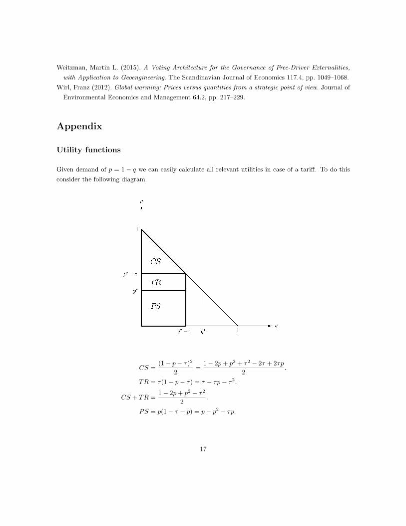
Given demand of p = 1 − q we can easily calculate all relevant utilities in case of a tariff. To do this

consider the following diagram.

CS =(1− p− τ)2

2=

1− 2p+ p2 + τ2 − 2τ + 2τp

2.

TR = τ(1− p− τ) = τ − τp− τ2.

CS + TR =1− 2p+ p2 − τ2

2.

PS = p(1− τ − p) = p− p2 − τp.

17

Country F taking pollution levels into account

Without foreign production

We briefly want to present a generalization of the model introduced in the second section, where both

countries care about pollution levels. That is, we let H solve

maxpt≥0gt≥0

∫ ∞0

e−rt[(pt − p

2t − τtpt

)−g2t2−αH2

(Pt − gt)2

]dt,

and country F solve

maxτt≥0

∫ ∞0

e−rt[

1

2(1− 2pt + p2t − τ

2t )− βgt −

αF2

(Pt − gt)2

]dt.

s.t.

Pt = qt − δPt = 1− pt − τt − δPt , P0 ≥ 0.

We allow for country specific damage-weights caused by increasing pollution levels and consequently

solve the game for Markov-perfect strategies. Due to their length closed form solutions are not reported

here but are available upon request. The general result obtained in section two still holds, i.e. ∂τt/∂β >

0,∀Pt but now due to αF 6= 0 there exists the possibility for a qualitative difference in the slope of

the optimal control functions. One can show that the slope of the optimal tariff changes sign at

αF := 12

(αH(1 + αH) + r2(1 + αH)2 −

√r2(1 + αH)3(r2 + (2 + r2)αH)

). Specifically,

ψ3

> 0, for αF < αF= 0, for αF = αF< 0, for αF > αF ,

where we had τt = −ψ2 − ψ3Pt. Hence, F chooses decreasing (increasing) tariffs over time if it suffers

relatively little (much) of increased pollution.

18

With foreign production

This setting implies for H

maxgt

∫ ∞0

e−rt[(1− qHt − q

Ft − τ

Ht )qHt −

g2t2−αH2

(Pt − gt)2

]dt,

and for F

maxτHt , τ

Ft

∫ ∞0

e−rt

[(qHt + qFt )2

2+ (1− qHt − q

Ft − τ

Ft )qFt + τHt q

Ht + τFt q

Ft − βgt −

αF2

(Pt − gt)2

]dt,

s.t.

Pt = qHt + qFt =2− τHt − τFt

3, P0 ≥ 0,

qHt =1− 2τHt + τFt

3, qFt =

1− 2τFt + τHt3

.

Again, it still holds that ∂τF,t/∂β > 0, ∂τH,t/∂β > 0, ∀Pt but since F also suffers from increasing

pollution levels it needs to reduce its own production over time. It does so by increasingly taxing

its own industry - no subsidy is given in that case. A typical set of optimal controls, the state and

production quantities are depicted in the following figure.

Figure 4: Optimal paths over time with r = 0.03, αH = αF = 0.02 and β = 0.2.

19