climate model emulation in an integrated assessment ... model emulation in an integrated assessment...

Earth Syst. Dynam., 7, 119–132, 2016

www.earth-syst-dynam.net/7/119/2016/

doi:10.5194/esd-7-119-2016

© Author(s) 2016. CC Attribution 3.0 License.

Climate model emulation in an integrated assessment

framework: a case study for mitigation policies in the

electricity sector

A. M. Foley1,a, P. B. Holden2, N. R. Edwards2, J.-F. Mercure1,b, P. Salas1, H. Pollitt3, and

U. Chewpreecha3

1Cambridge Centre for Climate Change Mitigation Research, Department of Land Economy, University of

Cambridge, 19 Silver Street, Cambridge, CB3 9EP, UK2Environment, Earth and Ecosystems, Open University, Milton Keynes, MK7 6AA, UK

3Cambridge Econometrics Ltd, Covent Garden, Cambridge, CB1 2HT, UKanow at: Department of Geography, Environment and Development Studies, Birkbeck, University of London,

32 Tavistock Square, London, WC1H 9EZ, UKbnow at: Department of Environmental Sciences, Radboud University, Nijmegen, the Netherlands

Correspondence to: A. M. Foley ([email protected])

Received: 22 June 2015 – Published in Earth Syst. Dynam. Discuss.: 4 August 2015

Revised: 7 January 2016 – Accepted: 12 January 2016 – Published: 15 February 2016

Abstract. We present a carbon-cycle–climate modelling framework using model emulation, designed for inte-

grated assessment modelling, which introduces a new emulator of the carbon cycle (GENIEem). We demonstrate

that GENIEem successfully reproduces the CO2 concentrations of the Representative Concentration Pathways

when forced with the corresponding CO2 emissions and non-CO2 forcing. To demonstrate its application as part

of the integrated assessment framework, we use GENIEem along with an emulator of the climate (PLASIM-

ENTSem) to evaluate global CO2 concentration levels and spatial temperature and precipitation response pat-

terns resulting from CO2 emission scenarios. These scenarios are modelled using a macroeconometric model

(E3MG) coupled to a model of technology substitution dynamics (FTT), and represent different emissions re-

duction policies applied solely in the electricity sector, without mitigation in the rest of the economy. The effect

of cascading uncertainty is apparent, but despite uncertainties, it is clear that in all scenarios, global mean tem-

peratures in excess of 2 ◦C above pre-industrial levels are projected by the end of the century. Our approach

also highlights the regional temperature and precipitation patterns associated with the global mean temperature

change occurring in these scenarios, enabling more robust impacts modelling and emphasizing the necessity of

focusing on spatial patterns in addition to global mean temperature change.

1 Introduction

Integrated assessment modelling can be used to explore the

climatic consequences of particular climate mitigation pol-

icy scenarios. However, most integrated assessment mod-

els (IAMs) do not directly utilize sophisticated coupled At-

mosphere Ocean General Circulation Models, such as those

employed in the Coupled Model Intercomparison Project

Phase 5 (CMIP5: Friedlingstein et al., 2014), to represent the

climate and carbon cycle. Due to the large computational re-

sources they require, the direct use of such models within

IAMs is not feasible.

Instead, many IAMs have used simple mechanistic models

to represent the carbon cycle. One such simplified carbon-

cycle/climate model is MAGICC6 (Meinshausen et al.,

2011a), which is calibrated against higher-complexity mod-

els from the Coupled Carbon Cycle Climate Model Intercom-

parison Project (C4MIP), to emulate the atmospheric CO2

concentrations of those models. Schaeffer et al. (2015) used

MAGICC6 to derive probability distributions for radiative

Published by Copernicus Publications on behalf of the European Geosciences Union.

120 A. M. Foley et al.: Integrated assessment using model emulation

forcing, which drive a simple climate model that projects

global mean temperature response by linearly scaling the

CO2 step experiment response of 17 CMIP5 General Circu-

lation Model (GCM) 4×CO2 simulations. Such approaches

can be used to generate large ensembles quite quickly; for in-

stance, MAGICC6 has been used to generate a 600-member

perturbed parameter ensemble (Schaeffer et al., 2015) of

CO2-equivalent concentration and global mean surface air

temperature change projections.

It has been suggested that a conceptual advantage of this

approach is that the mechanistic model fit adds some con-

fidence when extrapolating beyond the training data (Mein-

shausen et al., 2011a). A limitation of simplified mechanistic

models is that they may contain a high level of parametriza-

tion. For example, the Meinshausen et al. (2011a) carbon cy-

cle calibration procedure uses global mean temperature as a

proxy for changes in patterns of temperature and precipita-

tion. These drivers of change in the carbon cycle would be

explicitly represented in a more sophisticated model.

To represent regionally varying patterns of climatic

change, as opposed to global mean temperature change,

many IAM studies have used pattern scaling (e.g. IMAGE:

Bouwman et al., 2006). This computationally inexpensive

technique linearly relates regional climatic change, derived

from stored GCM ensembles such as those generated in

CMIP5, to global mean temperature change, simulated us-

ing a simplified model, so that the regional response to many

emissions scenarios can be computed quickly (e.g. Cabré

et al., 2010). Simple pattern scaling assumes that the cli-

mate response is spatially invariant (with respect to time

and forcing), and therefore cannot capture aspects which

may be sensitive to the greenhouse gas (GHG) concentra-

tion pathway (O’Neill and Oppenheimer, 2004; Tebaldi and

Arblaster, 2014). Tebaldi and Arblaster (2014) cite a number

of instances where it is liable to break down, in particular

for scenarios with strong mitigation or less mean tempera-

ture change. Recent advances in pattern scaling have consid-

ered the effects of different forcing components; for example,

with the most recent iteration of MAGICC-SCENGEN, the

effects of aerosols can be estimated for some climate param-

eters by generating patterns specific to these emissions1.

The Atmosphere–Ocean General Circulation

Model (AOGCM) ensembles used in pattern scaling

are usually multi-model ensembles (MMEs). Such ensem-

bles consist of simulations from different models, and are

neither a systematic nor random sampling of potential future

climates (Tebaldi and Knutti, 2007). Similarities between

models may lead to a lack of independence amongst

ensemble members (Foley et al., 2013), complicating the

interpretation of the ensemble as a whole (Knutti et al.,

2013).

1MAGICC/SCENGEN user manual, p. 2: http://www.cgd.ucar.

edu/cas/wigley/magicc/UserMan5.3.v2.pdf.

Perturbed physics ensembles (PPEs) offer a more system-

atic sampling of potential future climates, but embedding a

PPE approach into an IAM framework requires a computa-

tionally fast climate model. In this context, statistical emu-

lation of complex models is a useful alternative. For exam-

ple, Castruccio et al. (2014) constructed a statistical climate

model emulator using simulations performed with the Com-

munity Climate System Model, version 3 (CCSM3), in which

statistical models are fitted to temperature and precipitation

for 47 subcontinental-scale regions. Such an approach is suit-

able for applications requiring annual temperatures of spe-

cific regions, but is less appropriate when climate impacts

within regions are to be considered. Carslaw et al. (2013) ap-

ply a similar approach to the grid cell level. However, such

an approach requires many emulators, and correspondingly,

computational resources. Furthermore, the global emulation

may not be self-consistent, as the individual emulators do not

utilize the correlations between grid cells.

In this paper, we demonstrate how model emulation us-

ing singular vector decomposition (SVD) can be used within

an IAM framework to generate PPEs, systematically captur-

ing uncertainty in the future climate state while also pro-

viding insight into regional climate change. We introduce

the GENIEem-PLASIM-ENTSem (GPem) climate–carbon-

cycle emulator, which consists of a statistical climate model

emulator, PLASIM-ENTSem, to represent climate dynamics

(Holden et al., 2014), and a new carbon cycle emulator GE-

NIEem. Compared to a simple mechanistic model, the purely

statistical GENIEem does not impose a predefined functional

structure, allowing the emulator to capture more of the be-

haviour of the underlying simulator, and notably providing

a representation of the parametric uncertainty of the simula-

tor. Although parametric uncertainty of MAGICC itself can

be investigated (Meinshausen et al., 2009), this is distinct

from representing the parametric uncertainties and associ-

ated non-linear feedbacks in the underlying simulator. Simi-

larly, compared to pattern scaling, the more complex statisti-

cal approach used in PLASIM-ENTSem enables a represen-

tation of spatial uncertainties due to parametric uncertainties

in the underlying model. The use of SVD to decompose spa-

tial patterns of climate parameters makes PLASIM-ENTSem

computationally efficient, compared to techniques in which

statistical relationships are developed for each grid cell.

We demonstrate how these emulators can be applied in an

IAM framework to resolve the regional environmental im-

pacts associated with policy scenarios by coupling GPem to

FTT:Power-E3MG, a non-equilibrium economic model with

a technology diffusion component. Our work builds on that

of Labriet et al. (2015) and Joshi et al. (2015) who also de-

rived IAMs from economic and energy technology system

models coupled to PLASIM-ENTSem.

Earth Syst. Dynam., 7, 119–132, 2016 www.earth-syst-dynam.net/7/119/2016/

http://www.cgd.ucar.edu/cas/wigley/magicc/UserMan5.3.v2.pdf

http://www.cgd.ucar.edu/cas/wigley/magicc/UserMan5.3.v2.pdf

A. M. Foley et al.: Integrated assessment using model emulation 121

2 The GENIEem carbon cycle model emulator

The carbon cycle model emulator GENIEem is an emulator

of the GENIE-1 Earth System Model (ESM) (Holden et al.,

2013a) (i.e. a statistical model that approximately reproduces

selected outputs from the full GENIE-1 ESM). The emulator

takes a time series of anthropogenic carbon emissions and

non-CO2 radiative forcing (stemming from CH4, N2O, halo-

carbons, and other forcing agents including O3 and aerosols)

as inputs and provides a time series of atmospheric CO2 con-

centration as output.

In the integrated assessment framework developed here,

the time series of anthropogenic carbon emissions is pro-

vided by E3MG-FTT, while non-CO2 forcing data are de-

rived from global time series of forcing data obtained

through the RCP Database2. As such, GPem emulates high-

dimensional climate outputs as a function of scalar model in-

puts (Holden et al., 2015). We note that certain forcings, such

as aerosol forcing, are characterized by complex spatial pat-

terns and so would benefit from an approach in which the in-

puts are also high dimensional. However, incorporating such

forcing into the emulator framework would involve coupling

an aerosol model to PLASIM-ENTS in order to build an en-

semble of simulations and a subsequent emulator, which is

beyond the current scope of this work.

2.1 GENIE-1 description

The full GENIE-1 ESM comprises the 3-D frictional

geostrophic ocean model GOLDSTEIN (Edwards and

Marsh, 2005) coupled to a 2-D Energy Moisture Balance At-

mosphere based on that of Fanning and Weaver (1996) and

Weaver et al. (2001), and a thermodynamic–dynamic sea-ice

model based on Semtner (1976) and Hibler (1979). Ocean

biogeochemistry is modelled with BIOGEM (Ridgwell et al.,

2007), coupled to the sediment model SEDGEM (Ridgwell

and Hargreaves, 2007). GENIE-1 is run at 36×36 spatial res-

olution (≈ 10◦× 5◦ on average) with an≈1-day atmospheric

time step, and 16 depth levels in the ocean. Vegetation is

simulated with ENTSML (Holden et al., 2013a), a dynamic

model of terrestrial carbon and land use change (LUC) based

on the single plant functional type model ENTS (Williamson

et al., 2006). ENTSML takes time-varying fields of LUC as

inputs. Each simulation used to build the emulator is a tran-

sient simulation from AD 850 through to 2105. Historical

forcing (AD 850 to 2005), including changing land use, is

prescribed as described in Eby et al. (2013). Future forcing

(2005 to 2105) is defined by a CO2 concentration time series

and a non-CO2 radiative forcing time series, both represented

by polynomials (see Sect. 2.1.2). The LUC mask is held fixed

from 2005, as capturing LUC–climate–carbon feedbacks in

the emulator would require high-dimensional inputs, a signif-

2Data available via the RCP Database at http://tntcat.iiasa.ac.at:

8787/RcpDb.

icantly more complex ensemble design and emulation chal-

lenge. The future forcing due to LUC is instead subsumed

into the CO2 concentration (LUC emissions) and non-CO2

radiative forcing (LUC albedo).

The configuration is the same as that applied in the Earth

system model of intermediate complexity (EMIC) intercom-

parison project (Zickfeld et al., 2013). Due to its reduced

complexity, GENIE-1 is a good choice for performing the

many simulations required to build an emulator.

2.2 GENIE-1 parameter set selection

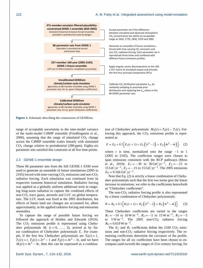
Construction of GENIEem is summarized in (Fig. 1). To

build the carbon cycle emulator, a subset of the 471-member

emulator filtered plausibility-constrained parameter sets de-

scribed in Holden et al. (2013b) is used. Each of these 471 pa-

rameter sets was previously applied to a CO2 emissions-

forced transient historical simulation (AD 850 to 2005). They

comprise experiments 1 and 2 of Holden et al. (2013a). In ad-

dition to emissions forcing, these simulations were forced by

non-CO2 trace gases, LUC, anthropogenic aerosols, volcanic

aerosols, orbital change and solar variability, as described in

Eby et al. (2013).

The 471 parameter sets are constrained to be plausible in

the preindustrial state by design (Holden et al., 2013b). How-

ever, they are not constrained to be plausible in the present

day as neither the anthropogenic carbon sinks nor the LUC

emissions are calibrated. Additionally, these 471 parameter

sets are known to contain members that display numerical

instabilities (Holden et al., 2013a).

In order to identify useful parameter sets, we apply a filter

to this transient historical ensemble. A parameter set is ac-

cepted as plausible if the difference between simulated and

observed atmospheric CO2 concentration lies within an ac-

ceptable range at each of five time points, AD 1620, 1770,

1850, 1970 and 2005:

|CO2(t)−CO∗2(t)|<

√ε2

0 + ε2t , (1)

where CO2(t) and CO∗2(t) are simulated and observed atmo-

spheric CO2 concentration, evaluated at each time slice t , and

the acceptable errors ε0 and εt relate to the preindustrial spin-

up state and to the transient change. The time points span

the preindustrial period and are not associated with volcanic

eruptions as these can lead to an unrealistic carbon cycle re-

sponse in GENIE due to the single-layer soil module (Holden

et al., 2013a).

The ε0 term dominates the acceptable error during the

preindustrial era and is designed to reject any simulations

that exhibit numerical instability. It is set equal to 2 SD (stan-

dard deviations) (9 ppm) of the 471-member spin-up ensem-

ble. The εt term is given by 0.22× (CO∗2(t)− 280) ppm. This

term dominates the acceptable error in the post-industrial era

and is designed to reject simulations that exhibit an unreason-

able strength for the CO2 sink. It approximately limits the

www.earth-syst-dynam.net/7/119/2016/ Earth Syst. Dynam., 7, 119–132, 2016

http://tntcat.iiasa.ac.at:8787/RcpDb



Accept parameter set if the difference between simulated and observed atmospheric CO2 concentration lies within an acceptable range at 1620, 1770, 1850, 1970 and 2005.

Generate an ensemble of future simulations , forced with time-varying CO2 emissions and non-CO2 radiative forcing. Each parameter set is reproduced three times and combined with different future emissions profiles.

Calibrate CO2 fertilisation parameter k14 by randomly sampling its assumed prior distribution and replacing the k14 values in the 86 GENIE parameter sets.

Apply singular vector decomposition to the 100 x 257 matrix of simulated output and emulate the first four principal components (PCs).

Calibrated GENIEem climate/carbon cycle emulator

(generates an 86-member ensemble using GENIE-1 parameter sets, for six given Chebyshev coefficients)

471-member emulator filtered plausibility-constrained GENIE-1 ensemble (850-2005)

(transient historical emissions-forced ensemble, plausible in preindustrial state by design)

86 parameter sets from GENIE-1 (plausible in preindustrial period

and present day)

257-member 100-year (2005-2105) GENIE-1 future ensemble

(257 out of 258 simulations completed successfully)

Uncalibrated GENIEem climate/carbon cycle emulator

(generates an 86-member ensemble using GENIE-1 parameter sets, for six given Chebyshev coefficients)

Figure 1. Schematic describing the construction of GENIEem.

range of acceptable uncertainty to the inter-model variance

of the multi-model C4MIP ensemble (Friedlingstein et al.,

2006), assuming that the range of simulated CO2 change

across the C4MIP ensemble scales linearly with simulated

CO2 change relative to preindustrial (280 ppm). Eighty-six

parameter sets satisfied this constraint at all five time points.

2.3 GENIE-1 ensemble design

These 86 parameter sets from the full GENIE-1 ESM were

used to generate an ensemble of future simulations (2005 to

2105) forced with time-varying CO2 emissions and non-CO2

radiative forcing. Each simulation was continued from its

respective transient historical simulation. Radiative forcing

was applied as a globally uniform additional term in outgo-

ing long-wave radiation to capture the combined effects of

non-CO2 trace gases, aerosols and LUC on global tempera-

ture. The LUC mask was fixed at the 2005 distribution, but

effects of future land use changes are accounted for, albeit

approximately, in the applied radiative forcing and emissions

anomalies.

To capture the range of possible future forcing we

followed the approach of Holden and Edwards (2010).

The CO2 emissions profile is represented using Cheby-

shev polynomials Mi (i= 0, . . . , 3), arrived at by lin-

ear combination of Chebyshev polynomials Ti . For exam-

ple, if the first few Chebyshev polynomials are T0(t)= 1,

T1(t)= t , T2(t)= 2t2− 1 and T3(t)= 4t3− 3t , and we have

M3(t)= 4t3− 4t , then this can be expressed as a combina-

tion of Chebyshev polynomials: M3(t)= T3(t)− T1(t). Fol-

lowing this approach, the CO2 emissions profile is repre-

sented as

E = E0+ 0.5[E1(t + 1)+E2

(2t2− 2

)+E3

(4t3− 4t

)], (2)

where t is time, normalized onto the range −1 to 1

(2005 to 2105). The coefficient ranges were chosen to

span emissions consistent with the RCP pathways (Moss

et al., 2010): E1=−30 to 30 GtC yr−1, E2=−15 to

15 GtC yr−1, E3=−15 to 15 GtC yr−1. The 2005 emissions

E0= 9.166 GtC yr−1.

Note that Eq. (2) is strictly a linear combination of Cheby-

shev polynomials such that the first two terms give the linear

increase in emissions; we refer to the coefficients henceforth

as “Chebyshev coefficients”.

The non-CO2 radiative forcing profile is also represented

by a linear combination of Chebyshev polynomials:

R = R0+ 0.5[R1(t + 1)+R2

(2t2− 2

)+R3

(4t3− 4t

)]. (3)

These Chebyshev coefficients are varied in the ranges

R1=−10 to 10 W m−2, R2=−5 to 15 W m−2, R3=−5

to 5 W m−2. The 2005 non-CO2 radiative forcing

R0= 0.619 W m−2.

The E1 and R1 coefficients define the 2100 CO2 emis-

sions and non-CO2 radiative forcing respectively. The re-

maining coefficients determine the curvature of the profile.

The ranges for all six coefficients have been chosen to en-

compass (and exceed) the ranges of 21st century forcing; for



emulator training we apply wider ranges than we expect to

need in order to ensure the emulator is never used under ex-

trapolation. Selecting a broad training range helps to ensure

that the emulator will remain suitable for use in many dif-

ferent applications, and not only within the context of the

scenarios studied in this work.

For example, the maximumE1= 30 gives 2100 CO2 emis-

sions of E0+E1= 39.166 GtC, which compares to RCP8.5

emissions of 28.817 GtC. Maximum radiative forcing of

R0+R1= 10.619 W m−2 was allowed to greatly exceed

RCP estimates (maximum 1.796 W m−2) in order to allow

the potential application of the emulator to extreme non-

CO2 forcing scenarios, for instance to represent non-CO2

(e.g. methane) runaway feedbacks (Schmidt and Shindell,

2003) or geo-engineering in a high-CO2 future (Irvine et al.,

2009).

The 86 parameter sets were replicated three times, and

each of these three 86-parameter sets were combined with

different future emissions profiles to produce a 258-member

ensemble. To achieve this, the six coefficients were varied

over the above ranges to create a 258-member Maximin Latin

Hypercube design, using the maximinLHS function of the lhs

package in R (R Development Core Team, 2013) – 257 sim-

ulations completed; in the remaining simulation, input pa-

rameters led to an unphysical state and ultimately, numerical

instability.

2.4 Construction of GENIEem

The emulation approach closely follows the dimension re-

duction methodology detailed in Holden et al. (2014). We

have an ensemble of 257 transient simulations of the coupled

climate–carbon system, incorporating both parametric uncer-

tainty (28 parameters) and forcing uncertainty (six modified

Chebyshev coefficients). For coupling applications we re-

quire an emulator that will generate the annually resolved

evolution of CO2 concentration through time (2006 to 2105).

The simulation outputs were combined into a (100× 257)

matrix Y, and SVD was performed on the matrix

Y= LDRT (4)

where L is the (100× 257) matrix of left singular vectors

(“component”), D is the 257× 257 diagonal matrix of the

square roots of the eigenvalues and R is the 257× 257 matrix

of right singular vectors (“component scores”).

We retain the first four components, which together ex-

plain more than 99.9 % of the ensemble variance. Each indi-

vidual simulated CO2 concentration time series can thus be

well approximated as a linear combination of the first four

components, scaled by their respective scores. Each set of

scores consists of a vector of coefficients, representing the

projection of each simulation onto the respective component.

As each simulated time series is a function of the input pa-

rameters, so are the coefficients that comprise the scores. So

each component score can be viewed, and hence emulated,

as a scalar function of the input parameters to the simulator.

Emulators of the first four component scores were derived

as functions of the 28 model parameters and the six concen-

tration profile coefficients. These emulators were built in R

(R Development Core Team, 2013), using the stepAIC func-

tion (Venables and Ripley, 2002). For each emulator, we

first built a linear model from all 34 inputs allowing only

terms that satisfy the Bayes Information Criterion (BIC).

BIC-constrained stepwise addition of quadratic and cross-

terms was then performed, allowing only inputs present in

the linear model.

While the variance in emulator output is dominated by

the Chebyshev forcing coefficients, uncertainty for a given

forcing scenario is generated through emulator dependencies

on GENIE-1 parameters. The most important of these is the

CO2 fertilization parameter, k14, describing the uncertain re-

sponse of photosynthesis to changing CO2 concentrations.

To use the emulator, we constrain k14 using the calibration

of Holden et al. (2013a), to better quantify the uncertainty

associated with the terrestrial sink. We evaluate the resulting

emulated uncertainty through a comparison with C4MIP in

Sect. 2.6.

We approximate the prior as a normal distribution with

mean 500 ppm and standard deviation 150 ppm, following

the base posterior of Holden et al. (2013a). We sampled val-

ues at random from this distribution and replaced the k14 val-

ues in the 86-member training parameter set. Then, to gener-

ate a perturbed parameter ensemble of emulated futures, the

emulation is performed for each of the resulting 86 parameter

sets.

2.5 Validation of GENIEem

To validate the emulator, we apply leave-one-out cross-

validation, which involves rebuilding the emulator 257 times

with a different simulation omitted and comparing the omit-

ted simulation with its emulation. The proportion of vari-

ance VT explained by the emulator under cross-validation is

given by

VT = 1−

257∑n=1

100∑t=1

(Sn, t −En, t)2/

257∑n=1

100∑t=1

(Sn, t − St

)2, (5)

where S(n,t) is the simulated CO2 concentration at time t in

left-out ensemble member n, E(n,t) the corresponding emu-

lated output and St is the ensemble mean output at time t .

VT measures the degree to which individual emulations can

be regarded as accurate (Holden et al., 2014)

The cross-validated root mean square error of the emulator

is given by

RMSE=

√√√√ 257∑n=1

100∑t=1

(Sn, t −En, t)2

25 700. (6)



202020402060 208021000

20

40

60

80

100

Year

CO

2 con

cent

ratio

n (p

pm)

RCP 2.6

202020402060 208021000

50

100

150

200

250

Year

CO

2 con

cent

ratio

n (p

pm)

RCP 4.5

2020 204020602080 21000

100

200

300

Year

CO

2 con

cent

ratio

n (p

pm)

RCP 6.0

2020 204020602080 21000

200

400

600

Year

CO

2 con

cent

ratio

n (p

pm)

RCP 8.5

Emulator median CO2 concentrations

Emulator range of CO2 concentrations

RCP CO2 concentrations

CMIP5 median CO2 concentrations for RCP 8.5

CMIP5 range of CO2 concentrations for RCP 8.5

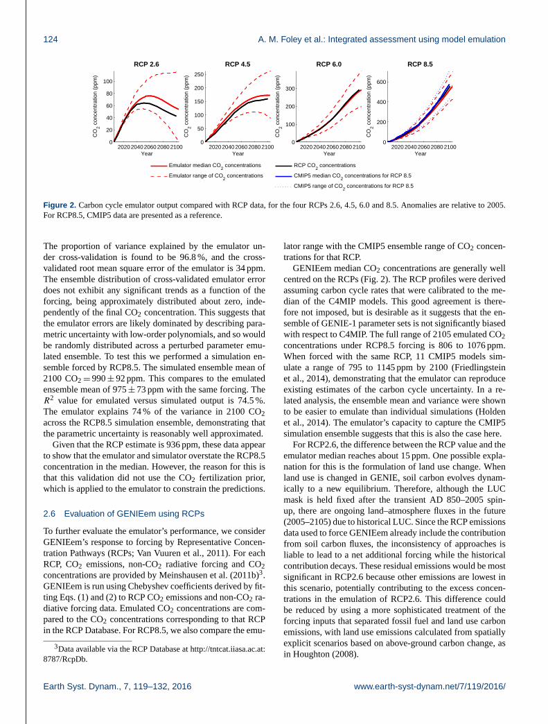
Figure 2. Carbon cycle emulator output compared with RCP data, for the four RCPs 2.6, 4.5, 6.0 and 8.5. Anomalies are relative to 2005.

For RCP8.5, CMIP5 data are presented as a reference.

The proportion of variance explained by the emulator un-

der cross-validation is found to be 96.8 %, and the cross-

validated root mean square error of the emulator is 34 ppm.

The ensemble distribution of cross-validated emulator error

does not exhibit any significant trends as a function of the

forcing, being approximately distributed about zero, inde-

pendently of the final CO2 concentration. This suggests that

the emulator errors are likely dominated by describing para-

metric uncertainty with low-order polynomials, and so would

be randomly distributed across a perturbed parameter emu-

lated ensemble. To test this we performed a simulation en-

semble forced by RCP8.5. The simulated ensemble mean of

2100 CO2= 990± 92 ppm. This compares to the emulated

ensemble mean of 975± 73 ppm with the same forcing. The

R2 value for emulated versus simulated output is 74.5 %.

The emulator explains 74 % of the variance in 2100 CO2

across the RCP8.5 simulation ensemble, demonstrating that

the parametric uncertainty is reasonably well approximated.

Given that the RCP estimate is 936 ppm, these data appear

to show that the emulator and simulator overstate the RCP8.5

concentration in the median. However, the reason for this is

that this validation did not use the CO2 fertilization prior,

which is applied to the emulator to constrain the predictions.

2.6 Evaluation of GENIEem using RCPs

To further evaluate the emulator’s performance, we consider

GENIEem’s response to forcing by Representative Concen-

tration Pathways (RCPs; Van Vuuren et al., 2011). For each

RCP, CO2 emissions, non-CO2 radiative forcing and CO2

concentrations are provided by Meinshausen et al. (2011b)3.

GENIEem is run using Chebyshev coefficients derived by fit-

ting Eqs. (1) and (2) to RCP CO2 emissions and non-CO2 ra-

diative forcing data. Emulated CO2 concentrations are com-

pared to the CO2 concentrations corresponding to that RCP

in the RCP Database. For RCP8.5, we also compare the emu-

3Data available via the RCP Database at http://tntcat.iiasa.ac.at:

8787/RcpDb.

lator range with the CMIP5 ensemble range of CO2 concen-

trations for that RCP.

GENIEem median CO2 concentrations are generally well

centred on the RCPs (Fig. 2). The RCP profiles were derived

assuming carbon cycle rates that were calibrated to the me-

dian of the C4MIP models. This good agreement is there-

fore not imposed, but is desirable as it suggests that the en-

semble of GENIE-1 parameter sets is not significantly biased

with respect to C4MIP. The full range of 2105 emulated CO2

concentrations under RCP8.5 forcing is 806 to 1076 ppm.

When forced with the same RCP, 11 CMIP5 models sim-

ulate a range of 795 to 1145 ppm by 2100 (Friedlingstein

et al., 2014), demonstrating that the emulator can reproduce

existing estimates of the carbon cycle uncertainty. In a re-

lated analysis, the ensemble mean and variance were shown

to be easier to emulate than individual simulations (Holden

et al., 2014). The emulator’s capacity to capture the CMIP5

simulation ensemble suggests that this is also the case here.

For RCP2.6, the difference between the RCP value and the

emulator median reaches about 15 ppm. One possible expla-

nation for this is the formulation of land use change. When

land use is changed in GENIE, soil carbon evolves dynam-

ically to a new equilibrium. Therefore, although the LUC

mask is held fixed after the transient AD 850–2005 spin-

up, there are ongoing land–atmosphere fluxes in the future

(2005–2105) due to historical LUC. Since the RCP emissions

data used to force GENIEem already include the contribution

from soil carbon fluxes, the inconsistency of approaches is

liable to lead to a net additional forcing while the historical

contribution decays. These residual emissions would be most

significant in RCP2.6 because other emissions are lowest in

this scenario, potentially contributing to the excess concen-

trations in the emulation of RCP2.6. This difference could

be reduced by using a more sophisticated treatment of the

forcing inputs that separated fossil fuel and land use carbon

emissions, with land use emissions calculated from spatially

explicit scenarios based on above-ground carbon change, as

in Houghton (2008).





3 Application of GPem in an IAM framework

To demonstrate the utility of emulation within an integrated

assessment framework, we describe how GENIEem, along

with PLASIM-ENTSem, has been used to explore the cli-

mate change implications of four policy scenarios for the

electricity sector, as presented in Mercure et al. (2014).

GPem is coupled to FTT:Power-E3MG, which combines

a technology diffusion model with a non-equilibrium eco-

nomic model. Mercure et al. (2014) emphasizes the policy in-

struments that can be applied to decarbonization of the global

energy sector, and analysis of climate impacts is limited to

mean surface temperature anomalies. Here, we extend that

work to illustrate the regional patterns of climate variability

associated with different policy scenarios, and discuss these

results in the context of “dangerous climate change” (Jarvis

et al., 2012).

3.1 The climate model emulator: PLASIM-ENTSem

PLASIM-ENTSem is an emulator of the GCM PLASIM-

ENTS; both simulator and emulator are described by Holden

et al. (2014). The GCM consists of a climate model, PLASIM

(Fraedrich, 2012), coupled to a simple surface and vegeta-

tion model, ENTS (Williamson et al., 2006), which repre-

sents vegetation and soil carbon through a single plant func-

tional type. PLASIM has a heat-flux-corrected slab ocean

and a mixed-layer of a given depth, and a 3-D dynamic atmo-

sphere, run at T21∼ 5◦ resolution. It utilizes primitive equa-

tions for vorticity, divergence, temperature and the logarithm

of surface pressure, solved via the spectral transform method,

and contains parametrizations for long- and short-wave ra-

diation, interactive clouds, moist and dry convection, large-

scale precipitation, boundary layer fluxes of latent and sensi-

ble heat and vertical and horizontal diffusion. It accounts for

water vapour, carbon dioxide and ozone.

As an emulator of PLASIM-ENTS, PLASIM-ENTSem

emulates mean fields of change for surface air temperature

and precipitation well, while emulations of precipitation un-

derestimate simulated ensemble variability, explaining∼ 60–

80 % of the variance in precipitation (compared to∼ 95 % for

surface air temperature) (Holden et al., 2014).

The response of PLASIM-ENTSem to RCP forcing was

analysed in Holden et al. (2014, Fig. 6); in all four scenar-

ios, the emulated ensemble distribution was found to com-

pare favourably with the multi-model CMIP5 ensemble.

3.2 Policy scenarios and emissions profiles

FTT:Power is a simulation model of the global power sec-

tor (Mercure, 2012), which has been coupled to a dynamic

simulation model of the global economy, E3MG (Mercure

et al., 2014)4. These models are described in greater de-

tail in the supplementary information of this paper. Policies

4www.4cmr.group.cam.ac.uk/research/FTT/fttviewer

2020 2040 2060 2080 21000

5

10

15

20

25

30

CO2 emissions profiles

Year

CO

2 em

issi

ons

(GtC

yr−

1 )

Scenario iScenario iiScenario iiiScenario ivRCP 4.5RCP 8.5

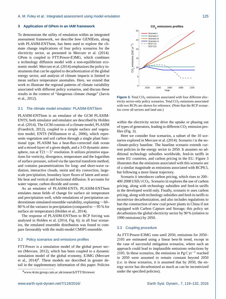
Figure 3. Total CO2 emissions associated with four different elec-

tricity sector-only policy scenarios. Total CO2 emissions associated

with two RCPs are shown for reference. (Note that the RCP scenar-

ios cover all sectors and land use.)

within the electricity sector drive the uptake or phasing out

of types of generators, leading to different CO2 emission pro-

files (Fig. 3).

Here we consider four scenarios, a subset of the 10 sce-

narios explored in Mercure et al. (2014). Scenario i is the no-

climate-policy baseline. The baseline scenario extends cur-

rent policies in the energy sector to 2050. It assumes no ad-

ditional technology subsidies worldwide, feed-in tariffs in

some EU countries, and carbon pricing in the EU. Figure 3

illustrates that the emissions associated with this scenario are

of a similar magnitude as emissions associated with RCP8.5,

but following a more linear trajectory.

Scenario ii introduces carbon pricing, which rises to 200–

400 2008 USD/tCO2. Scenario iii explores the use of carbon

pricing, along with technology subsidies and feed-in tariffs

in the developed world only. Finally, scenario iv uses carbon

pricing, along with technology subsidies and feed-in tariffs to

incentivize decarbonization, and also includes regulations to

ban the construction of new coal power plants in China if not

equipped with Carbon Capture and Storage; this policy set

decarbonizes the global electricity sector by 90 % (relative to

1990 emissions) by 2050.

3.3 Coupling procedure

As FTT:Power-E3MG runs until 2050, emissions for 2050–

2105 are estimated using a linear best-fit trend, except in

the case of successful mitigation scenarios, where such an

approach could lead to implausible emissions reductions by

2105. In these scenarios, the emissions in Pg C yr−1 reached

in 2050 were assumed to remain constant beyond 2050

(i.e. in these scenarios, it is assumed that by 2050, the en-

ergy sector has decarbonized as much as can be incentivized

under the specified policies).


www.4cmr.group.cam.ac.uk/research/FTT/fttviewer


Chebyshev coefficients are calculated to provide least-

squares fits to each emissions profile produced by

FTT:Power-E3MG. If we conservatively assume that any er-

ror in emissions due to differences between the FTT:Power-

E3MG emissions profile and the corresponding Chebyshev

curve has an infinite lifetime in the atmosphere, the accumu-

lated error does not exceed 4.5 ppm in any scenario over the

period 2005–2105, well within the 5th–95th percentiles of

GENIEem.

As FTT:Power-E3MG does not simulate non-CO2 ra-

diative forcing, we select the RCP that best matches

the CO2 concentrations associated with the baseline sce-

nario (RCP8.5) and force GENIEem with the non-CO2 radia-

tive forcing associated with that RCP. The RCP8.5 non-CO2

radiative forcing was applied to all scenarios as the RCPs

lack a suitable analog to the CO2 concentrations associated

with the power sector mitigation scenarios examined in this

work. Values for Chebyshev coefficients are calculated and

these three coefficients, together with the three CO2 emis-

sions coefficients, are the inputs to GENIEem.

This approach maintains comparability across the differ-

ent scenarios, although we expect some small reductions in

CH4 and N2O in the mitigation scenarios, due to a reduc-

tion in leaks of these GHGs from drilling. Representations

of these GHGs in E3MG-FTT are not sufficiently detailed to

provide forcing data for GPem, but reductions in fuel-use-

related CH4 and N2O emissions of around 10–15 % by 2050

in the mitigation scenarios can be inferred. After 2050, we

expect a stabilization at this new level, as the sectors involved

have decarbonized by 90 %, producing a reduction in forc-

ing of roughly 0.1 Wm−2 (relative to total forcing of 7.3 to

8.3 W m−2 in the baseline and 5.3 to 6.2 W m−2 in the mit-

igation scenario, accounting for carbon cycle uncertainty).

This small reduction in forcing is well within the uncertainty

bounds of GENIEem.

Climate–carbon feedbacks are emulated entirely within

GENIEem. No climate information is passed from PLASIM-

ENTSem to GENIEem. PLASIM-ENTSem takes inputs of

both actual CO2 (for CO2 fertilization) and equivalent CO2

(for radiative forcing). Chebyshev coefficients are calculated

to provide least-squares fits to the median and 5th–95th

percentiles of the GENIEem ensemble CO2 concentrations;

these coefficients, therefore, correspond to actual CO2 con-

centrations. Chebyshev coefficients for equivalent CO2 are

also calculated, corresponding to combined CO2 and non-

CO2 forcings. To determine these coefficients for equivalent

CO2, the median and 5th–95th percentiles of the GENIEem

ensemble CO2 concentrations are converted to radiative forc-

ing following

1F = 5.35ln(CO2/280) Wm−2. (7)

RCP8.5 non-CO2 forcing is added to this time series to give

total radiative forcing, which is converted to equivalent CO2

using the previous relationship. Chebyshev coefficients for

equivalent CO2 are fitted to the resulting time series.

Thus, PLASIM-ENTSem is forced with three sets of six

coefficients (three actual CO2 and three equivalent CO2 each

for the median and 5th–95th percentiles of the GENIEem en-

semble).

We calculate the median warming of the PLASIM-

ENTSem ensemble based on the 5th and 95th percentiles of

the GENIEem ensemble. These bounds, therefore, illustrate

parametric uncertainty of the carbon cycle model alone.

We also calculate the median and 5th–95th percentiles of

warming of the PLASIM-ENTSem ensemble from the me-

dian GENIEem ensemble output. These bounds reflect para-

metric uncertainty in the climate model alone.

Finally, we calculate the 5th percentile of warming from

the PLASIM-ENTSem ensemble based on the 5th percentile

of CO2 concentration from the GENIEem ensemble, and the

95th percentile of warming from the PLASIM-ENTSem en-

semble based on the 95th percentile of CO2 concentration

from the GENIEem ensemble. This third set of bounds re-

flects warming uncertainty due to parametric uncertainty in

the climate model and the carbon cycle model, computed un-

der the assumption that GENIEem and PLASIM-ENTSem

projections are perfectly correlated, i.e. that states exhibit-

ing the greatest CO2 concentration in GENIEem correspond

to states exhibiting greatest warming in PLASIM-ENTSem.

Many carbon cycle processes are affected directly by changes

in temperature, or by variables which covary with tempera-

ture (Willeit et al., 2014), so while such a correlation is not

absolute, there is a motivation for this approach.

4 Results

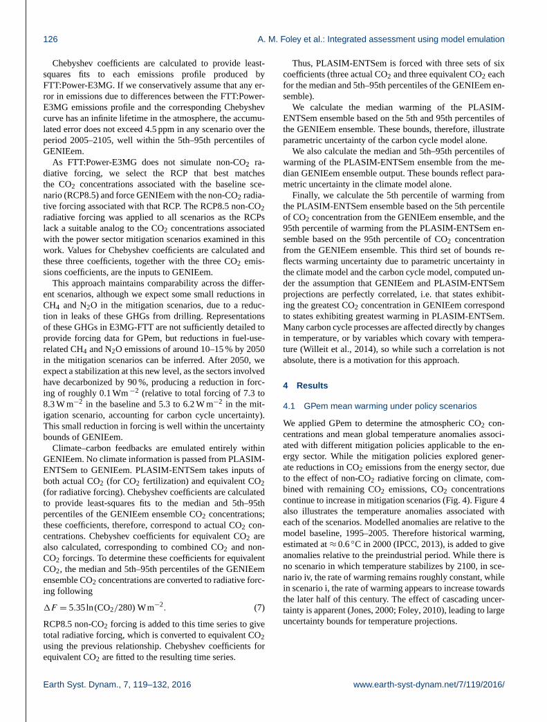
4.1 GPem mean warming under policy scenarios

We applied GPem to determine the atmospheric CO2 con-

centrations and mean global temperature anomalies associ-

ated with different mitigation policies applicable to the en-

ergy sector. While the mitigation policies explored gener-

ate reductions in CO2 emissions from the energy sector, due

to the effect of non-CO2 radiative forcing on climate, com-

bined with remaining CO2 emissions, CO2 concentrations

continue to increase in mitigation scenarios (Fig. 4). Figure 4

also illustrates the temperature anomalies associated with

each of the scenarios. Modelled anomalies are relative to the

model baseline, 1995–2005. Therefore historical warming,

estimated at ≈ 0.6 ◦C in 2000 (IPCC, 2013), is added to give

anomalies relative to the preindustrial period. While there is

no scenario in which temperature stabilizes by 2100, in sce-

nario iv, the rate of warming remains roughly constant, while

in scenario i, the rate of warming appears to increase towards

the later half of this century. The effect of cascading uncer-

tainty is apparent (Jones, 2000; Foley, 2010), leading to large

uncertainty bounds for temperature projections.



Figure 4. Top panels: median CO2 concentrations for scenarios i (baseline), ii, iii and iv, simulated by GENIEem, with uncertainty bounds

(GENIEem 5th/95th percentile). Bottom panels: median temperature anomalies relative to preindustrial conditions for scenarios a (baseline),

d, i and j, simulated by PLASIM-ENTSem using median GENIEem CO2 concentrations. Uncertainty bounds are based on carbon cycle

uncertainty (PLASIMem median with GENIEem 5th/95th percentile), climate uncertainty (PLASIMem 5th/95th percentile with GENIEem

median), and combined uncertainty (PLASIMem 5th/95th percentile with GENIEem 5th/95th percentile). The 2 ◦C target, described as “the

maximum allowable warming to avoid dangerous anthropogenic interference in the climate” (e.g Randalls, 2010), is also illustrated by the

grey dashed line.

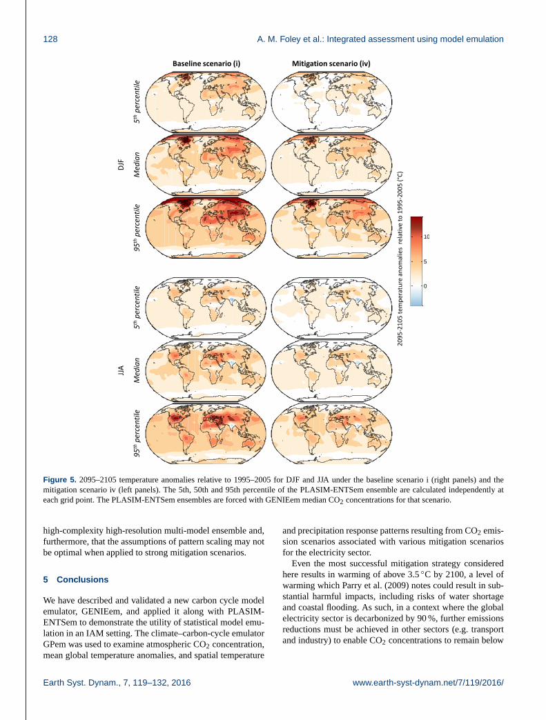
4.2 GPem regional climate under policy scenarios

Figure 5 illustrates the 2095–2105 December–February and

June–August warming anomalies associated with scenario i

and iv, presenting the median and 5th/95th percentiles of

the PLASIM-ENTSem ensemble outputs calculated indepen-

dently at each grid point. These emulated ensembles are

forced with GENIEem median CO2 concentrations for the

respective scenario, giving an indication of the range of

PLASIM-ENTSem parametric uncertainty associated with

the projection. It is evident that the warming associated with

the baseline scenario would be partially offset under the mit-

igation scenario. However, certain hotspots of warming are

apparent even under the 5th percentile projection. In both

scenarios, there is cooling in Southeast Asia in summer,

which likely arises due to a strengthening of the monsoon

in PLASIM-ENTSem. However, Holden et al. (2014) note

that this signal may not be robust as the model lacks aerosol

forcing.

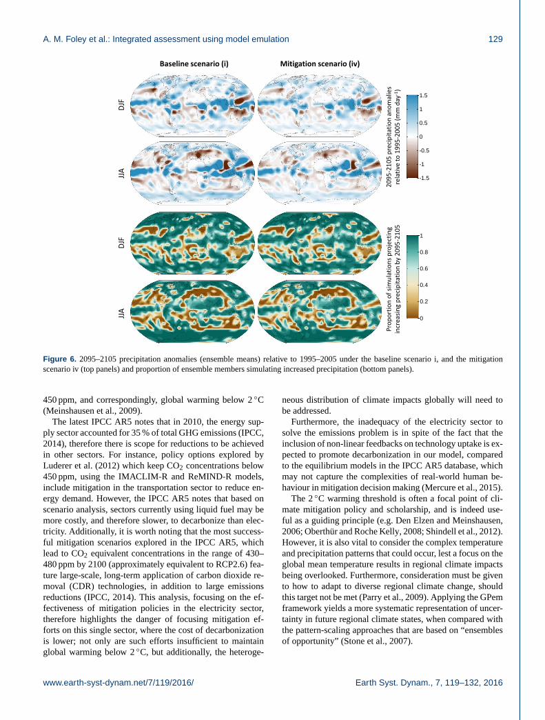
Figure 6 illustrates the mean 2095–2105 December–

February and June–August precipitation patterns associated

with scenarios i and iv, along with the proportion of the

86 ensemble members simulating increased precipitation in

each case. Generally, areas that experience a significant in-

crease/decrease in precipitation under scenario iv (i.e. larger

than ±1 mm day−1) experience even greater extremes under

scenario i, which can be attributed to differences in water

vapour amount in the atmosphere due to warming (Held and

Soden, 2006); precipitation fields are amplified as more wa-

ter is available in the convergence zones to condense. Plotting

the proportion of ensemble members that project increasing

precipitation shows that in most regions of the world, there is

high agreement between ensemble members on the direction

of change for precipitation.

Precipitation patterns are similar for the two scenarios pre-

sented (r = 0.99), suggesting that a simple pattern scaling

approach would have sufficed in the particular example con-

sidered here, at least for estimation of the ensemble mean

field. However, Tebaldi and Arblaster (2014) considered cor-

relations between the averaged precipitation anomaly fields

(2090–1990) of the CMIP5 multi-model ensemble when

forced with different RCPs; the lowest correlation (0.85)

was between ensembles forced with RCP2.6 and RCP8.5,

while a correlation of 0.97 was found between RCP4.5

and RCP8.5. Applying our emulation framework yielded

correlations of 0.89–0.93 (RCP2.6, RCP8.5) and 0.97–0.98

(RCP4.5, RCP8.5), depending on season. This comparison

suggests that the emulation framework captures non-linear

feedback strengths that are comparable to those found in a



Baseline scenario (i) Mitigation scenario (iv)

DJF

5th

per

cen

tile

M

edia

n

95

th p

erce

nti

le

JJA

5th

per

cen

tile

M

edia

n

95

th p

erce

nti

le

20

95

-21

05

tem

per

atu

re a

no

mal

ies

rel

ativ

e to

19

95

-20

05

(°C

)

0

5

10

Figure 5. 2095–2105 temperature anomalies relative to 1995–2005 for DJF and JJA under the baseline scenario i (right panels) and the

mitigation scenario iv (left panels). The 5th, 50th and 95th percentile of the PLASIM-ENTSem ensemble are calculated independently at

each grid point. The PLASIM-ENTSem ensembles are forced with GENIEem median CO2 concentrations for that scenario.

high-complexity high-resolution multi-model ensemble and,

furthermore, that the assumptions of pattern scaling may not

be optimal when applied to strong mitigation scenarios.

5 Conclusions

We have described and validated a new carbon cycle model

emulator, GENIEem, and applied it along with PLASIM-

ENTSem to demonstrate the utility of statistical model emu-

lation in an IAM setting. The climate–carbon-cycle emulator

GPem was used to examine atmospheric CO2 concentration,

mean global temperature anomalies, and spatial temperature

and precipitation response patterns resulting from CO2 emis-

sion scenarios associated with various mitigation scenarios

for the electricity sector.

Even the most successful mitigation strategy considered

here results in warming of above 3.5 ◦C by 2100, a level of

warming which Parry et al. (2009) notes could result in sub-

stantial harmful impacts, including risks of water shortage

and coastal flooding. As such, in a context where the global

electricity sector is decarbonized by 90 %, further emissions

reductions must be achieved in other sectors (e.g. transport

and industry) to enable CO2 concentrations to remain below



Baseline scenario (i) Mitigation scenario (iv)

DJF

JJ

A

DJF

JJ

A

Pro

po

rtio

n o

f si

mu

lati

on

s p

roje

ctin

g in

crea

sin

g p

reci

pit

atio

n b

y 2

09

5-2

10

5

-1.5

-1

-0.5

0

0.5

1

1.5

JJA (j)

0

0.2

0.4

0.6

0.8

1

20

95

-21

05

pre

cip

itat

ion

an

om

alie

s

rela

tive

to

19

95

-20

05

(m

m d

ay-1

)

Figure 6. 2095–2105 precipitation anomalies (ensemble means) relative to 1995–2005 under the baseline scenario i, and the mitigation

scenario iv (top panels) and proportion of ensemble members simulating increased precipitation (bottom panels).

450 ppm, and correspondingly, global warming below 2 ◦C

(Meinshausen et al., 2009).

The latest IPCC AR5 notes that in 2010, the energy sup-

ply sector accounted for 35 % of total GHG emissions (IPCC,

2014), therefore there is scope for reductions to be achieved

in other sectors. For instance, policy options explored by

Luderer et al. (2012) which keep CO2 concentrations below

450 ppm, using the IMACLIM-R and ReMIND-R models,

include mitigation in the transportation sector to reduce en-

ergy demand. However, the IPCC AR5 notes that based on

scenario analysis, sectors currently using liquid fuel may be

more costly, and therefore slower, to decarbonize than elec-

tricity. Additionally, it is worth noting that the most success-

ful mitigation scenarios explored in the IPCC AR5, which

lead to CO2 equivalent concentrations in the range of 430–

480 ppm by 2100 (approximately equivalent to RCP2.6) fea-

ture large-scale, long-term application of carbon dioxide re-

moval (CDR) technologies, in addition to large emissions

reductions (IPCC, 2014). This analysis, focusing on the ef-

fectiveness of mitigation policies in the electricity sector,

therefore highlights the danger of focusing mitigation ef-

forts on this single sector, where the cost of decarbonization

is lower; not only are such efforts insufficient to maintain

global warming below 2 ◦C, but additionally, the heteroge-

neous distribution of climate impacts globally will need to

be addressed.

Furthermore, the inadequacy of the electricity sector to

solve the emissions problem is in spite of the fact that the

inclusion of non-linear feedbacks on technology uptake is ex-

pected to promote decarbonization in our model, compared

to the equilibrium models in the IPCC AR5 database, which

may not capture the complexities of real-world human be-

haviour in mitigation decision making (Mercure et al., 2015).

The 2 ◦C warming threshold is often a focal point of cli-

mate mitigation policy and scholarship, and is indeed use-

ful as a guiding principle (e.g. Den Elzen and Meinshausen,

2006; Oberthür and Roche Kelly, 2008; Shindell et al., 2012).

However, it is also vital to consider the complex temperature

and precipitation patterns that could occur, lest a focus on the

global mean temperature results in regional climate impacts

being overlooked. Furthermore, consideration must be given

to how to adapt to diverse regional climate change, should

this target not be met (Parry et al., 2009). Applying the GPem

framework yields a more systematic representation of uncer-

tainty in future regional climate states, when compared with

the pattern-scaling approaches that are based on “ensembles

of opportunity” (Stone et al., 2007).



While uncertainties associated with carbon cycle and cli-

mate modelling in this framework are accounted for through

the use of ensembles, it is still possible that the actual future

climate state may fall outside the simulated range. Uncer-

tainties associated with emissions profiles are more difficult

to quantify as these depend, ultimately, on human decision

making. Therefore many policy contexts should be modelled

in order to find out which ones effectively lead to desired

outcomes.

The Supplement related to this article is available online

at doi:10.5194/esd-7-119-2016-supplement.

Acknowledgements. We acknowledge the support of

D. Crawford-Brown. We thank F. Babonneau for providing

code to generate Chebyshev coefficients, P. Friedlingstein for

provision of CMIP5 data and M. Syddall for his advice regarding

data visualization. This work was supported by the Three Guineas

Trust (A. M. Foley), the EU Seventh Framework Programme grant

agreement no. 265170 “ERMITAGE” (N. Edwards and P. Holden),

the UK Engineering and Physical Sciences Research Council, fel-

lowship number EP/K007254/1 (J.-F. Mercure), Conicyt (Comisión

Nacional de Investigación Científica y Tecnológica, Gobierno de

Chile) and the Ministerio de Energía, Gobierno de Chile (P. Salas),

and Cambridge Econometrics (H. Pollitt and U. Chewpreecha).

Edited by: J. Dyke

References

Bouwman, A. F., Kram, T., and Klein Goldewijk, K.: Integrated

modelling of global environmental change. An overview of

IMAGE 2.4, Netherlands Environmental Assessment Agency,

Bilthoven, the Netherlands, 2006.

Cabré, M. F., Solman, S., and Nuñez, M.: Creating regional climate

change scenarios over southern South America for the 2020s and

2050s using the pattern scaling technique: Validity and limita-

tions, Climatic Change, 98, 449–469, 2010.

Carslaw, K. S., Lee, L. A., Reddington, C. L., Pringle, K. J., Rap,

A., Forster, P. M., Mann, G. W., Spracklen, D. V., Woodhouse,

M. T., Regayre, L. A., and Pierce, J. R.: Large contribution of

natural aerosols to uncertainty in indirect forcing, Nature, 503,

67–71, 2013.

Castruccio, S., McInerney, D. J., Stein, M. L., Liu Crouch, F., Ja-

cob, R. L., and Moyer, E. J.: Statistical emulation of climate

model projections based on precomputed gcm runs, J. Climate,

27, 1829–1844, 2014.

Den Elzen, M. and Meinshausen, M.: Meeting the EU 2 ◦C climate

target: Global and regional emission implications, Clim. Policy,

6, 545–564, 2006.

Eby, M., Weaver, A. J., Alexander, K., Zickfeld, K., Abe-Ouchi, A.,

Cimatoribus, A. A., Crespin, E., Drijfhout, S. S., Edwards, N. R.,

Eliseev, A. V., Feulner, G., Fichefet, T., Forest, C. E., Goosse, H.,

Holden, P. B., Joos, F., Kawamiya, M., Kicklighter, D., Kienert,

H., Matsumoto, K., Mokhov, I. I., Monier, E., Olsen, S. M., Ped-

ersen, J. O. P., Perrette, M., Philippon-Berthier, G., Ridgwell, A.,

Schlosser, A., Schneider von Deimling, T., Shaffer, G., Smith, R.

S., Spahni, R., Sokolov, A. P., Steinacher, M., Tachiiri, K., Tokos,

K., Yoshimori, M., Zeng, N., and Zhao, F.: Historical and ide-

alized climate model experiments: an intercomparison of Earth

system models of intermediate complexity, Clim. Past, 9, 1111–

1140, doi:10.5194/cp-9-1111-2013, 2013.

Edwards, N. R. and Marsh, R.: Uncertainties due to transport-

parameter sensitivity in an efficient 3-d ocean-climate model,

Clim. Dynam., 24, 415–433, 2005.

Fanning, A. F. and Weaver, A. J.: An atmospheric energy-moisture

balance model: Climatology, interpentadal climate change, and

coupling to an ocean general circulation model, J. Geophys. Res.-

Atmos., 101, 15111–15128, 1996.

Foley, A.: Uncertainty in regional climate modelling: A review,

Prog. Phys. Geogr., 34, 647–670, 2010.

Foley, A., Fealy, R., and Sweeney, J.: Model skill measures in prob-

abilistic regional climate projections for Ireland, Clim. Res., 56,

33–49, 2013.

Fraedrich, K.: A suite of user-friendly global climate models: Hys-

teresis experiments, Eur. Phys. J. Plus, 127, 1–9, 2012.

Friedlingstein, P., Cox, P., Betts, R., Bopp, L., Von Bloh, W.,

Brovkin, V., Cadule, P., Doney, S., Eby, M., Fung, I., Bala, G.,

John, J., Jones, C., Joos, F., Kato, F., Kawamiya, M., Knorr,

W., Lindsay, K., Matthews, H., Raddatz, T., Rayner, P., Reick,

C., Roeckner, E., Schnitzler, K. G., Schnur, R., Strassman, K.,

Weaver, A., Yoshikawa, C., and Zeng, N.: Climate-carbon cycle

feedback analysis: Results from the C4MIP model intercompari-

son, J. Climate, 19, 3337–3353, 2006.

Friedlingstein, P., Meinshausen, M., Arora, V. K., Jones, C. D.,

Anav, A., Liddicoat, S. K., and Knutti, R.: Uncertainties in

CMIP5 climate projections due to carbon cycle feedbacks, J. Cli-

mate, 27, 511–526, 2014.

Held, I. M. and Soden, B. J.: Robust responses of the hydrological

cycle to global warming, J. Climate, 19, 5686–5699, 2006.

Hibler, W.: A dynamic thermodynamic sea ice model, J. Phys.

Oceanogr., 9, 815–846, 1979.

Holden, P. B. and Edwards, N.: Dimensionally reduced emulation of

an AOGCM for application to integrated assessment modelling,

Geophys. Res. Lett., 37, L21707, doi:10.1029/2010GL045137,

2010.

Holden, P. B., Edwards, N. R., Gerten, D., and Schaphoff, S.: A

model-based constraint on CO2 fertilisation, Biogeosciences, 10,

339–355, doi:10.5194/bg-10-339-2013, 2013a.

Holden, P. B., Edwards, N. R., Müller, S. A., Oliver, K. I. C.,

Death, R. M., and Ridgwell, A.: Controls on the spatial dis-

tribution of oceanic δ13CDIC, Biogeosciences, 10, 1815–1833,

doi:10.5194/bg-10-1815-2013, 2013b.

Holden, P. B., Edwards, N. R., Garthwaite, P. H., Fraedrich, K.,

Lunkeit, F., Kirk, E., Labriet, M., Kanudia, A., and Babonneau,

F.: PLASIM-ENTSem v1.0: a spatio-temporal emulator of future

climate change for impacts assessment, Geosci. Model Dev., 7,

433–451, doi:10.5194/gmd-7-433-2014, 2014.

Holden, P. B., Edwards, N. R., Garthwaite, P. H., and Wilkinson,

R. D.: Emulation and interpretation of high-dimensional climate

model outputs, J. Appl. Stat., 42, 1–18, 2015.

Houghton, R.: Carbon flux to the atmosphere from land-use changes

1850–2005, in: TRENDS: A compendium of data on global


http://dx.doi.org/10.5194/esd-7-119-2016-supplement

http://dx.doi.org/10.5194/cp-9-1111-2013

http://dx.doi.org/10.1029/2010GL045137

http://dx.doi.org/10.5194/bg-10-339-2013

http://dx.doi.org/10.5194/bg-10-1815-2013

http://dx.doi.org/10.5194/gmd-7-433-2014


change, carbon dioxide information analysis center, Oak Ridge

National Laboratory, US Department of Energy, Oak Ridge,

Tenn., USA, 2008.

IPCC: Summary for Policymakers, in: Climate Change 2013: The

Physical Science Basis, Contribution of Working Group I to the

Fifth Assessment Report of the Intergovernmental Panel on Cli-

mate Change, edited by: Stocker, T., Qin, D., Plattner, G., Tig-

nor, M., Allen, S., Boschung, J., Nauels, A., Xia, Y., Bex, V., and

Midgley, P., Cambridge University Press, Cambridge, UK and

New York, NY, USA, 2013.

IPCC: Climate Change 2014: Mitigation of Climate Change, in:

Contribution of Working Group III to the Fifth Assessment Re-

port of the Intergovernmental Panel on Climate Change, edited

by: Edenhofer, O., Pichs-Madruga, R., Sokona, Y., Farahani, E.,

Kadner, S., Seyboth, K., Adler, A., Baum, I., Brunner, S., Eick-

emeier, P., Kriemann, B., Savolainen, J., Schlömer, S., von Ste-

chow, C., Zwickel, T., and Minx, J., Cambridge University Press,

Cambridge, UK and New York, NY, USA, 2014.

Irvine, P. J., Lunt, D. J., Stone, E. J., and Ridgwell, A.: The fate of

the Greenland Ice Sheet in a geoengineered, high CO2 world, En-

viron. Res. Lett., 4, 045109, doi:10.1088/1748-9326/4/4/045109,

2009.

Jarvis, A., Leedal, D., and Hewitt, C.: Climate-society feedbacks

and the avoidance of dangerous climate change, Nat. Clim.

Change, 2, 668–671, 2012.

Jones, R. N.: Managing uncertainty in climate change projections

– issues for impact assessment, Climatic Change, 45, 403–419,

2000.

Joshi, S. R., Vielle, M., Babonneau, F., Edwards, N. R., and Holden,

P. B.: Physical and economic consequences of sea-level rise: A

coupled GIS and CGE analysis under uncertainties, Environ. Re-

sour. Econ., doi:10.1007/s10640-015-9927-8, in press, 2015.

Knutti, R., Masson, D., and Gettelman, A.: Climate model geneal-

ogy: Generation CMIP5 and how we got there, Geophys. Res.

Lett., 40, 1194–1199, 2013.

Labriet, M., Joshi, S. R., Kanadia, A., Edwards, N. R., and Holden,

P. B.: Worldwide impacts of climate change on energy for heat-

ing and cooling, Mitig. Adapt. Strat. Glob. Change, 20.7, 1111–

1136, doi:10.1007/s11027-013-9522-7, 2015.

Luderer, G., Bosetti, V., Jakob, M., Leimbach, M., Steckel, J. C.,

Waisman, H., and Edenhofer, O.: The economics of decarboniz-

ing the energy system, results and insights from the recipe model

intercomparison, Climatic Change, 114, 9–37, 2012.

Meinshausen, M., Meinshausen, N., Hare, W., Raper, S. C., Frieler,

K., Knutti, R., Frame, D. J., and Allen, M. R.: Greenhouse-gas

emission targets for limiting global warming to 2 ◦C, Nature,

458, 1158–1162, 2009.

Meinshausen, M., Raper, S. C. B., and Wigley, T. M. L.: Emulat-

ing coupled atmosphere-ocean and carbon cycle models with a

simpler model, MAGICC6 – Part 1: Model description and cal-

ibration, Atmos. Chem. Phys., 11, 1417–1456, doi:10.5194/acp-

11-1417-2011, 2011a.

Meinshausen, M., Smith, S. J., Calvin, K., Daniel, J. S., Kainuma,

M. L. T., Lamarque, J. F., Matsumoto, K., Montzka, S. A., Raper,

S. C. B., Riahi, K., and Thomson, A. G.: The RCP greenhouse

gas concentrations and their extensions from 1765 to 2300, Cli-

matic Change, 109, 213–241, 2011b.

Mercure, J. F.:FTT:Power : A global model of the power sector with

induced technological change and natural resource depletion, En-

ergy Policy, 48, 799–811, 2012.

Mercure, J. F., Pollitt, H., Chewpreecha, U., Salas, P., Foley, A.,

Holden, P., and Edwards, N.: The dynamics of technology dif-

fusion and the impacts of climate policy instruments in the de-

carbonisation of the global electricity sector, Energy Policy, 73,

686–700, 2014.

Mercure, J. F., Pollitt, H., Bassi, A., Viñuales, J., and Ed-

wards, N.: Braving the tempest: Methodological foundations

of policy-making in sustainability transitions, arXiv preprint

arXiv:150607432, 2015.

Moss, R. H., Edmonds, J. A., Hibbard, K. A., Manning, M. R., Rose,

S. K., Van Vuuren, D. P., Carter, T. R., Emori, S., Kainuma, M.,

Kram, T., and Meehl, G. A.: The next generation of scenarios for

climate change research and assessment, Nature, 463, 747–756,

2010.

Oberthür, S. and Roche Kelly, C.: EU leadership in international

climate policy: achievements and challenges, Int. Spectator., 43,

35–50, 2008.

O’Neill, B. C. and Oppenheimer, M.: Climate change impacts are

sensitive to the concentration stabilization path, P. Natl. Acad.

Sci. USA, 101, 16411–16416, 2004.

Parry, M., Lowe, J., and Hanson, C.: Overshoot, adapt and recover,

Nature, 458, 1102–1103, 2009.

Randalls, S.: History of the 2 ◦C climate target, Wiley Interdisci-

plinary Reviews: Climate Change, 1, 598–605, 2010.

R Development Core Team: R: A Language and Environment for

Statistical Computing, R Foundation for Statistical Computing,

Vienna, Austria, http://www.R-project.org (last access: 2 Febru-

ary 2016), 2013.

Ridgwell, A. and Hargreaves, J.: Regulation of atmospheric CO2

by deep-sea sediments in an Earth system model, Global Bio-

geochem. Cy., 21, GB2008, doi:10.1029/2006GB002764, 2007.

Ridgwell, A., Hargreaves, J. C., Edwards, N. R., Annan, J. D.,

Lenton, T. M., Marsh, R., Yool, A., and Watson, A.: Marine geo-

chemical data assimilation in an efficient Earth System Model

of global biogeochemical cycling, Biogeosciences, 4, 87–104,

doi:10.5194/bg-4-87-2007, 2007.

Schaeffer, M., Gohar, L., Kriegler, E., Lowe, J., Riahi, K., and

van Vuuren, D.: Mid-and long-term climate projections for frag-

mented and delayed-action scenarios, Technol. Forecast. Social

Change, 90, 257–268, doi:10.1016/j.techfore.2013.09.013, 2015.

Schmidt, G. A. and Shindell, D. T.: Atmospheric composition, ra-

diative forcing, and climate change as a consequence of a mas-

sive methane release from gas hydrates, Paleoceanography, 18,

doi:10.1029/2002PA000757, 2003.

Semtner, A. J.: A model for the thermodynamic growth of sea ice in

numerical investigations of climate, J. Phys. Oceanogr., 6, 379–

389, 1976.

Shindell, D., Kuylenstierna, J. C., Vignati, E., van Dingenen, R.,

Amann, M., Klimont, Z., Anenberg, S. C., Muller, N., Janssens-

Maenhout, G., Raes, F., and Schwartz, J.: Simultaneously mit-

igating near-term climate change and improving human health

and food security, Science, 335, 183–189, 2012.

Stone, D., Allen, M. R., Selten, F., Kliphuis, M., and Stott, P. A.:

The detection and attribution of climate change using an ensem-

ble of opportunity, J. Climate, 20, 504–516, 2007.


http://dx.doi.org/10.1088/1748-9326/4/4/045109

http://dx.doi.org/10.1007/s10640-015-9927-8

http://dx.doi.org/10.1007/s11027-013-9522-7

http://dx.doi.org/10.5194/acp-11-1417-2011

http://dx.doi.org/10.5194/acp-11-1417-2011

http://www.R-project.org

http://dx.doi.org/10.1029/2006GB002764

http://dx.doi.org/10.5194/bg-4-87-2007

http://dx.doi.org/10.1016/j.techfore.2013.09.013

http://dx.doi.org/10.1029/2002PA000757


Tebaldi, C. and Arblaster, J. M.: Pattern scaling: Its strengths and

limitations, and an update on the latest model simulations, Cli-

matic Change 122, 459–471, 2014.

Tebaldi, C. and Knutti, R.: The use of the multi-model ensemble

in probabilistic climate projections, Philos. T. Roy. Soc. A, 365,

2053–2075, 2007.

Van Vuuren, D. P., Edmonds, J., Kainuma, M., Riahi, K., Thomson,

A., Hibbard, K., Hurtt, G. C., Kram, T., Krey, V., Lamarque, J.

F., and Masui, T.: The representative concentration pathways: an

overview, Climatic Change, 109, 5–31, 2011.

Venables, W. N. and Ripley, B. D.: Modern applied statistics with S,

Springer-Verlag, New York, 2002.

Weaver, A. J., Eby, M., Wiebe, E. C., Bitz, C. M., Duffy, P. B.,

Ewen, T. L., Fanning, A. F., Holland, M. M., MacFadyen, A.,

Matthews, H. D., and Meissner, K. J.: The UVIC earth system

climate model: Model description, climatology, and applications

to past, present and future climates, Atmos.-Ocean, 39, 361–428,

2001.

Willeit, M., Ganopolski, A., Dalmonech, D., Foley, A. M., and Feul-

ner, G.: Time-scale and state dependence of the carbon-cycle

feedback to climate, Clim. Dynam., 42, 1699–1713, 2014.

Williamson, M., Lenton, T., Shepherd, J., and Edwards, N.: An effi-

cient numerical terrestrial scheme (ENTS) for Earth system mod-

elling, Ecol. Model., 198, 362–374, 2006.

Zickfeld, K., Eby, M., Weaver, A. J., Alexander, K., Crespin, E.,

Edwards, N. R., Eliseev, A. V., Feulner, G., Fichefet, T., For-

est, C. E., Friedlingstein, P., Goosse, H., Holden, P. B., Joos,

F., Kawamiya, M., Kicklighter, D., Kienert, H., Matsumoto, K.,

Mokhov, I. I., Monier, E., Olsen, S. M., Pedersen, J. O. P., Per-

rette, M., Philippon-Berthier, G., Ridgwell, A., Schlosser, A.,

Schneider Von Deimling, T., Shaffer, G., Sokolov, A., Spahni, R.,

Steinacher, M., Tachiiri, K., Tokos, K. S., Yoshimori, M., Zeng,

N., and Zhao, F.: Long-term climate change commitment and

reversibility: An EMIC intercomparison, J. Climate, 26, 5782–

5809, 2013.


climate model emulation in an integrated assessment ... model emulation in an integrated assessment...

Documents