climate modeling for global warming projection at … › aim › aim_workshop › ghg_2004 ›...

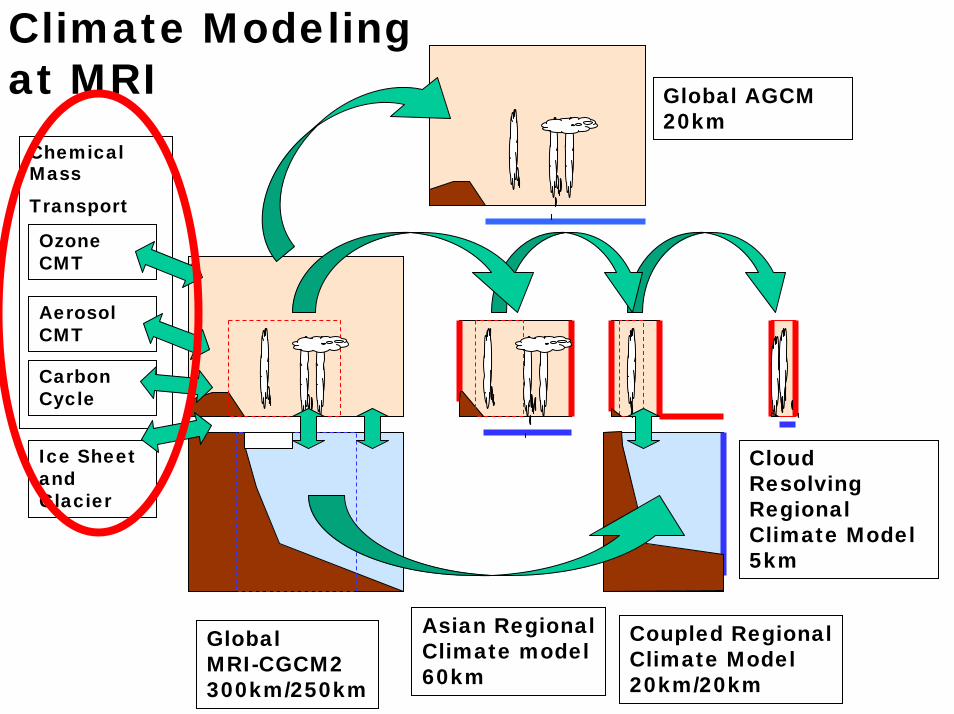
Climate Modeling for Global Warming Projection at the MRI

Akira Noda and MRI-CGCM modeling groupMeteorological Research Institute

• Transient runs with MRI-CGCMs• Downscaling with MRI regional

climate models• Earth system modeling for the

carbon cycle and chemical mass transport

Chemical Mass

Transport

Ozone CMT

Aerosol CMT

Carbon Cycle

Ice Sheet and Glacier

GlobalMRI-CGCM2300km/250km

Asian RegionalClimate model60km

Climate Modelingat MRI Global AGCM

20km

Cloud ResolvingRegional Climate Model5km

Coupled RegionalClimate Model20km/20km

• Feature MRI-CGCM1 MRI-CGCM2• Atmospheric component

• Horizontal resolution 5° (long.) x 4° (lat.) T42 (~2.8° x 2.8°)• Layers (top) 15 (1 hPa) 30 (0.4 hPa)• Solar radiation Lacis and Hansen (1974) Shibata and Uchiyama (1992)• (SW) H2O, O3 H2O, O3, CO2, O2aerosol• Long wave radiation Shibata and Aoki (1989) Shibata and Aoki (1989)• (LW) H2O, CO2, O3 H2O, CO2, O3, CH4, N2O• Convection Arakawa and Schubert (1974) Prognostic Arakawa-Schubert• Randall and Pan (1993)• Planetary Boundary Bulk layer (Tokioka et al., 1988) Mellor and Yamada (1974)• Layer (PBL)• Gravity wave drag Palmer et al. (1986) Iwasaki et al. (1989)• Rayleigh friction Rayleigh friction• Cloud type Penetrative convection, Penetrative convection• Middle-level convection,• Large-scale condensation, Large-scale condensation• stratus in PBL• Cloudiness Saturation Function of relative humidity• Cloud overlap Random for nonconsecutive clouds, Random + correlation• 0.3 for convective clouds• Cloud water content Function of pressure and Function of temperature• temperature• Land process 4-layer diffusion model 3-layer simple biosphere (SiB)

• Feature MRI-CGCM1 MRI-CGCM2• Oceanic component

• Horizontal resolution 2.5° (long) x 2° to 0.5° (lat) • Layers (min. thickness) 21 (5.2 m) 23 (5.2 m)• Eddy viscosity H. visc. 2.0 x 105 m2s–1 H. visc. 1.6 x 105 m2s–1

• V. visc. 1 x 10–4 m2s–1 V. visc. 1 x 10–4 m2s–1

• Eddy mixing Horizontal-vertical mixing Isopycnal mixing • + Gent and McWilliams (1990)• H. diff. 5.0 x 103 m2s–1 Isopycnal 2.0 x 103 m2s–1

• V. diff. 5.0 x 10–5m2s–1 Diapycnal 1.0 x 10–5 m2s–1

• Vertical viscosity and Mellor and Yamada (1974, 1982)• diffusivity•• Sea ice Mellor and Kantha (1989)•

• Atmosphere-ocean coupling• Coupling interval 6 hours 24 hours• Flux adjustment Heat, salinity Heat, salinity

+ wind stress (in the equatorial band 12°S to 12°N)

•

IPCC SRES and Stabilization Scenarios

A2A1BB2

MRI-CGCM2.3

(2071-2100) – (1961-1990))-（1961~1990）

変化パターンに大きな差は見られない。

MRI-CGCM2.3

Surface Air Temp. Change

Spatial patterns of Global Warming and Natural Variability

MRI-CGCMDue to CO2 increase

小

大

Due to El Nino

－

＋


Had-CGCMDue to CO2 increase

大

小

Due to El Nino

＋

－

Due to El Nino

＋

－

Due to CO2 increase

大

小

GFDL-CGCM


Mechanism of ENSO-like Change

EAST

Mechanism of ENSO ENSO-like Change

WARM

COLD

200ｍ

WEST

INDONESIAPERU

Walker circulation

Cane et al, 1997

Kitoh et al, 1999Knutson and Manabe,

1995,1998

Meehl and Washington, 1996

Mechanism of AO-like Change

Temp. dependence of moist adiabaitic laps rate

snow-ice meltstable stratification

Manabe and Wetherald (1975)

stronger snow/albedofeedback near the troughs

Noda et al. (1996)

Possible global warming patterns suggested by CGCMs

Observed trend

Comparison between Simulated AO-like and ENSO-like Changes

El Niño El NiñoSO ?

El Niño SO: La Niña

La Niña

AO CCSR/NIESHadCM3

ECHAM3/LSGECHAM4/OPYC3GFDL15

MRI1

Non-AO

CCCmaCSIROGFDL/R30HadCM2IPSLMRI2NCAR

Chemical Mass

Transport

Ozone CMT

Aerosol CMT

Carbon Cycle


Climate Modelingat MRI Global AGCM

20km





pCO2air

DICAlkalinityPhosphate

O2

insolationO2 saturation

∆pCO2 ×exchange coeff.

chemicalequilibrium

Carbon Cycle Model (included in MRI-CGCM)

New Production～Insolation×Phosphate

ParticulateOrganicMatter

CaCO3

deeplayer

e(−z/3500m

)

( z/100 m) −0 .9

106

106

9.5

9.5

16 19

1916

1

1

138

138

DIC

Advection andDiffusion by OGCM

surface layer (60m)

NPP (Temp., Precipitation)

leafbranch

stem

root

Ocean

litter

humus

stable humuscharcoal

1yr10yr

50yr

10yr

1yr

50yr

500yr

Atmosphere

pCO2sea

Phosphate

Alkalinity

O2

remineralizatio

n

dissolution

respiration

respiration

Ter r

est r

ial

Bi o

sphe

r e

Terrestrial Biosphere Model follows Goudriaan and Ketner (1984).NPP (Miami model: Lieth (1975), Friedlingstein et al. (1992)).

Ocean model by Obata (2001) and Obata and Kitamura (2003)

Ocean Carbon Cycle Model by Meteorological Research Institute

Climate change experiment 1961-1998 (driven by NCEP wind and JMA SST)

Figure:Sea-to-Air CO2 flux (in GtC/year)dashed line: global (variability (1std) = 0.23

GtC/yr)solid thick line: each region

Equatorial eastern Pacific (0.13 GtC/yr) is dominant by the ENSO (during El Niño, weak easterly, weak upwelling, reduced carbon supply from deeper waters and reduced sea-air CO2 flux).

Obata and Kitamura,Interannual variability of the sea-air exchange of CO2 from 1961 to 1998 ….., J. Geophys. Res., 108 (C11), 2003.

気象研海洋炭素循環モデルによる海洋大気間二酸化炭素交換の経年変動(1961-1998)

MRI model in 1976(pCO2air = 315ppm)

More detailed modelWoodward et al. (GBC, 1995)

Global amount =58 GtC/year

Net Primary Production(empirically determined from temperature andprecipitation, including pCO2air fertilization effect)

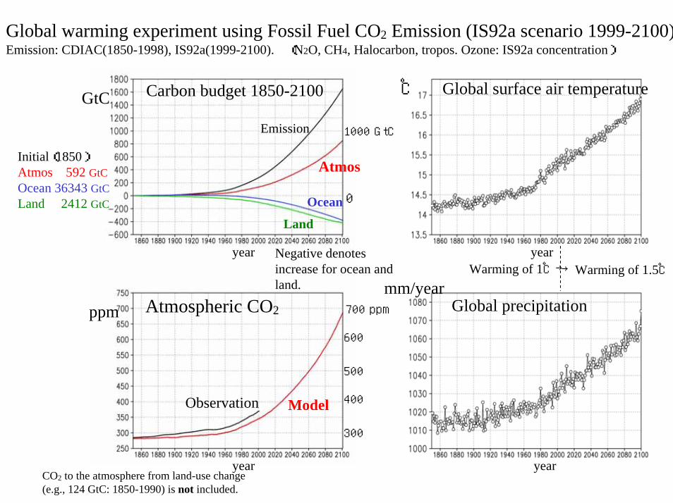
Global warming experiment using Fossil Fuel CO2 Emission (IS92a scenario 1999-2100)Emission: CDIAC(1850-1998), IS92a(1999-2100). （N2O, CH4, Halocarbon, tropos. Ozone: IS92a concentration）

Initial（1850）Atmos 592 GtCOcean 36343 GtCLand 2412 GtC

GtC Carbon budget 1850-2100

Emission

Atmos

Ocean

Land

1000 GtC

0

Model

℃

Warming of 1℃→→Warming of 1.5℃

700 ppm

500

600

400

300

year

Observation

Negative denotes increase for ocean and land.

Atmospheric CO2ppm

year

mm/yearGlobal precipitation

Global surface air temperature

year

yearCO2 to the atmosphere from land-use change (e.g., 124 GtC: 1850-1990) is not included.

Atlantic MeridionalCirculation related to NADW formation(Contour interval = 2×106m3/s)

Dep

th (m

)D

epth

(m)

Year: 1860

Year: 2100

Global warming experiment (IS92a CO2emission)

NADW is reduced by 20 %.18Sv↓14Sv

Chemical Mass

Transport

Ozone CMT

Aerosol CMT

Carbon Cycle



Global AGCM 20km

Climate Modelingat MRI




1981～2010 Present Climate

2041～2080 Warmed Climate

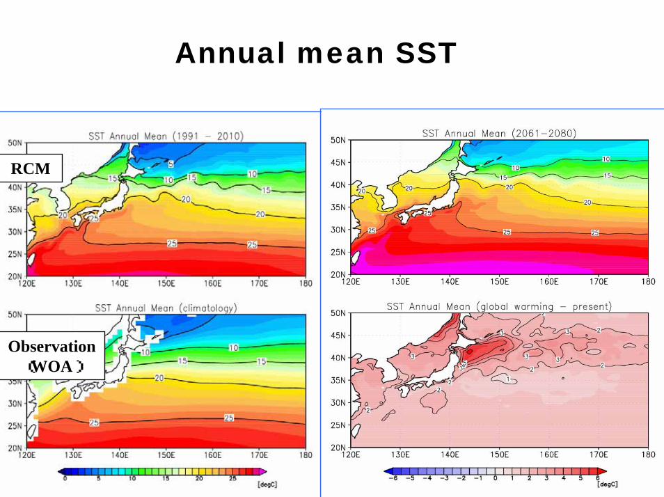
Annual mean SST

RCM

Observation（WOA）

Model TOPEX/Poseidon（1993-1999）

Dynamical sea level height (cm)

Chemical Mass

Transport

Ozone CMT

Aerosol CMT

Carbon Cycle


Global AGCM 20km

Climate Modelingat MRI





Earth Simulator

２０ｋｍメッシュ全球気候モデルによる現在気候の再現

１時間降水量(mm)

TL959による台風のシミュレーション

• 動画

Simulations of Tropical CyclonesWith AGCM of T106

Sugi, Noda and Sato(JMSJ, 2002)

More results are coming soon.

AcknowledgmentComputational resources are supplied by

MRI, CGER/NIES and Earth Simulator.

climate modeling for global warming projection at … › aim › aim_workshop › ghg_2004 ›...

Documents