Climate  of  an  Earth-­‐like  Aquaplanet:    the  high-­‐obliquity  case  and  the  <dally-­‐locked  case  David Ferreira, John Marshall Paul O’Gorman, Sara Seager,

Massachusetts Institute of Technology, Harriet Lau (Imperial College)

Why is the problem interesting from a climate dynamics perspective?

Climate of an aquaplanet at high obliquity

Tidally-locked aquaplanets

Earth-like planet with an atmosphere, an ocean and possibility of ice,

................but no land!

1

2

Outline

Conclusions

3

Our approach:

4

Coupled GCM +

Annual  mean  

January  

Incoming  solar  radia<on  

1. Why is the problem interesting from a climate dynamics perspective?

At high obliquity the poles are warmed more than the equator

Expect a reversal of pole-equator temperature gradient !!

Extreme seasonal cycle If polar temperatures are not to wildly fluctuate, heat must be stored or carried there.

Likely key role for the ocean

1

_ _ 23°_ _ 90°_ _ 54°_ _ 23°_ _ 90°_ _ 54°

Insolation for a tidally-locked Earth-like planet

•  Large and steady insolation contrast,

•  Outgoing long wave on night side.

èrequires a transport from day side to night side: Atmosphere and Ocean

èno role for storage in ocean

0 W/m^2 1300 W/m^2

Key  climate  ques<ons  

•   What determines the meridional energy transport and its partition between the atmosphere and ocean?

•   What is the role of the ocean in modulating extremes of temperature (through storage and transport)?

•   What determines the pattern of surface winds? - critical to ocean circulation (i.e. atmos angular mtm transport)

Earth-like planet …

Aqua Coupled GCM

… but without geometrical constraints

Atmosphere-only work: Joshi et al., 97; Joshi, 03; Williams and Kasting, 97; Williams and Pollard, 03; Merlis and Schneider, 2010; Showman et al. 2009; Heng and Vogt, 2011.

•  Primitive equation models,

•  Cube-sphere grid: ~3.75º, •  Synoptic scale eddies in the atmosphere,

•  Gent and McWilliams eddy parameterization in the ocean,

•  Simplified atmospheric physics (SPEEDY, Molteni 2003),

•  Conservation to numerical precision (Campin et al. 2008)

MIT GCM: Coupled Ocean-Atmosphere-Sea ice:

Poles well represented

Fully coupled: no adjustments Same grid for

ocean and atmosphere

Temperature snap-shot at 500 mb.

2

Aquaplanet  at  23.5  obliquity  

Climate of Aquaplanet

at obliquity of 23o

500mb T

Zonal jets in ocean

Equator

U

U

60N

Pattern of surface winds

W W

E

€

θA

€

θO

Marshall, Ferreira et al. (2007, J. Atmos. Sci.) Aquaplanet solution discussed in

SST & sea ice

Circumpolar currents

everywhere

30N

30S

60S

Pre

ssur

e D

epth

Today’s Earth climate

Energy transports in an Aquaplanet

Aquaplanet at 23.5° obliquity

-4

0

+4

PW

PW

Atm

Total

Ocn

- Patterns and magnitudes of transports are well captured in an Aquaplanet è to first order, continents are not necessary to explore the climate of an Earth-like planet

_ _ 23°_ _ 90°Annual means

Potential Temperature

3 Climate at high obliquity

Atmosphere

Ocean Ocean

Atmosphere

2 ºC 25 ºC

€

φ = 90o

€

φ = 23.5o

4 ºC 32 ºC

U

W W

E U W W

E

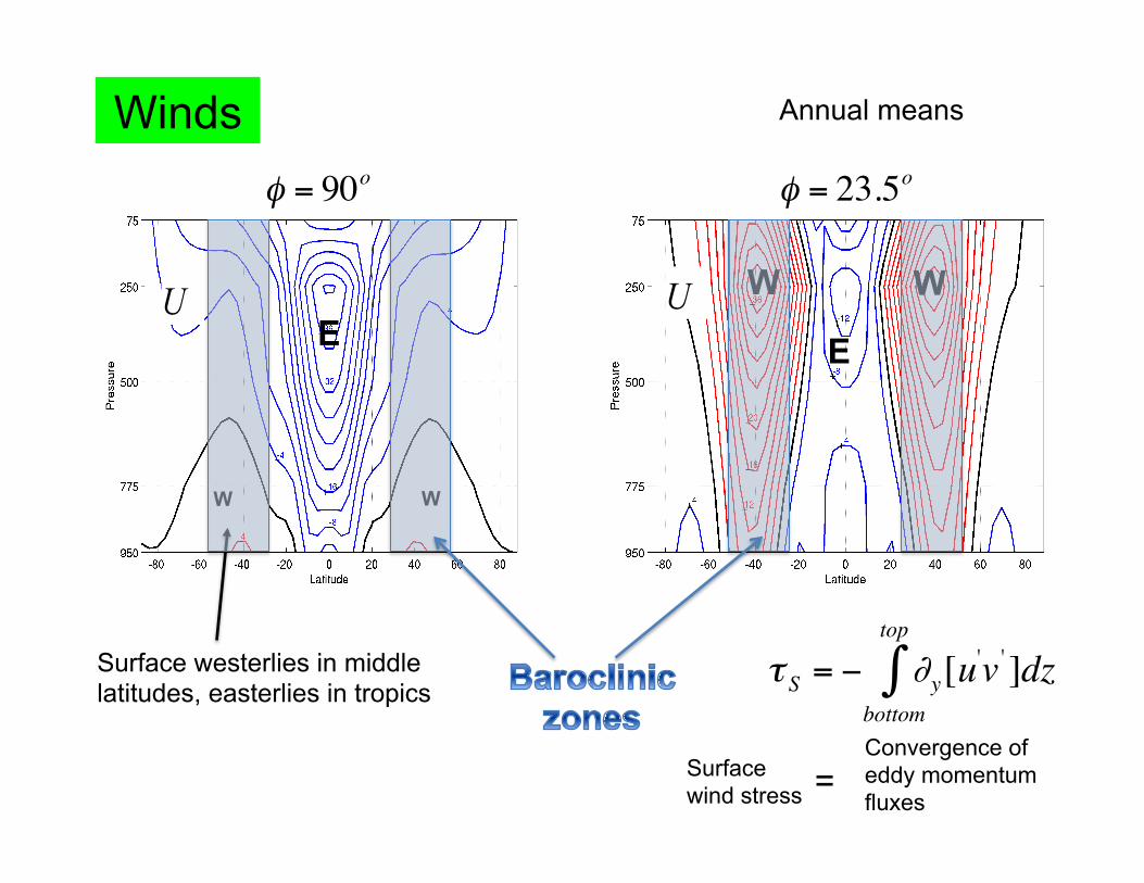
Winds

Surface westerlies in middle latitudes, easterlies in tropics

Annual means

€

τ S = − ∂y[u'v '

bottom

top

∫ ]dz

€

φ = 90o

€

φ = 23.5o

Surface wind stress =

Convergence of eddy momentum fluxes

(colors)

(contours)

waves

turbulence waves

turbulence

Asymmetries between easterly and westerly sheared flows

Eq Eq

E E

W W

W W EP = −u 'v ', f v 'θ '

θz

"

#$

%

&'

€

u'v '

€

U

€

q yβ

>>1

€

q yβ≈1

Eliassen-Palm fluxes:

€

φ = 90o

€

φ = 23.5o

Convective index

Strong surface temperature gradient in summer hemisphere (~40K) and weak gradient in winter hemisphere (~10K)

Seasonal variations restricted to top 200m --- amplitude of ~12K at pole --- almost steady and ~2K at equator

Atmosphere

Ocean _ _ 90°Seasonal Cycle

€

θA

€

θO

€

ΨO3000

Dep

th [m

]

Dep

th [m

]

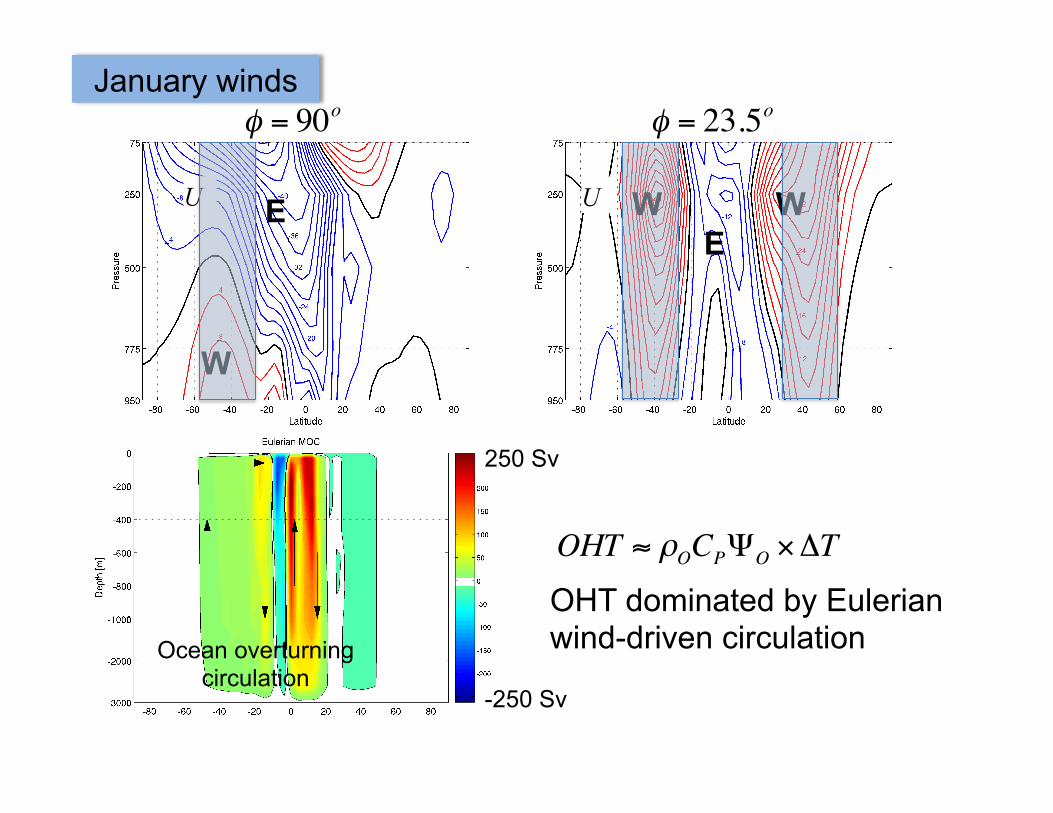
U U

January winds

W W

W

E E

Ocean overturning circulation

€

φ = 90o

€

φ = 23.5o

OHT ≈ ρOCPΨO ×ΔT

OHT dominated by Eulerian wind-driven circulation

250 Sv

-250 Sv

−50 0 50−2

0

2

4

6

8

10January

Eddy

Total

−50 0 50−2

0

2

4

6March

−50 0 50−6

−4

−2

0

2

4May

Atm. Heat Transport: Total and Eddy (=submonthly), Aqua Obli

−50 0 50−10

−8

−6

−4

−2

0

2July

January

Annual mean

Atmos and Ocean energy transport at high obliquity

_ _ 90°_ _ 90°Atm

Ocn

Atmosphere and Ocean heat transports are achieved seasonally: ----- large in the summer hemisphere ----- nearly vanish in the winter hemisphere

Equatorward transport everywhere ----- down large-scale temperature gradient

Total

Atm

Ocn

PW

0

12 +4

-4

Atmosphere

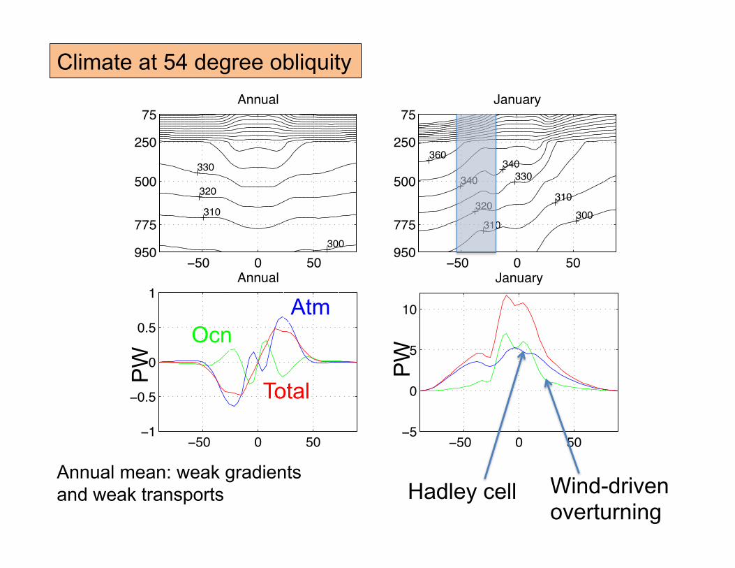
Climate at 54 degree obliquity

310

320

330

300

Annual

−50 0 50

75

250

500

775

950

310

320

340310

300

330340

360

January

−50 0 50

75

250

500

775

950

320

310

300

290

350340

March

−50 0 50

75

250

500

775

950

Potential temperature in K, Aqua Obli54 C24 Cpl362

320

330

310

300

340

300

May

−50 0 50

75

250

500

775

950

Fig. 8: Idem to Fig. 2 but for a 54◦ obliquity.

21

−50 0 50−1

−0.5

0

0.5

1Annual

−50 0 50−5

0

5

10

January

−50 0 50−5

0

5

10

March

Ocean and atmosphere energy Transports [PW]

−50 0 50−5

0

5

10

May

OHTAHTTotal

Fig. 10: Idem to Fig. 4 but for a 54◦ obliquity.

23

PW

PW

Atm Ocn

Total

Annual mean: weak gradients and weak transports Wind-driven

overturning Hadley cell

Tidally-locked Aquaplanet 4

Rossby radius = NHf=!"#

800 km (Atm) 50 km (Ocean)

at T=1 day

16000 km 1000 km at T=20 days

Surface air temperature:

T = 1 day T = 20 days

OLR

TOA OLR: ΔT = 63 K ΔT = 38 K

In W/m^2 ¤

¤ : Substellar point

¤ ¤

¤

Longitude

Latit

ude

T = 1 day T = 20 days

Surface ocean currents

Surface winds

Merlis and Schneider, 2010; Showman and Polvani 2011, Heng and Vogt, 2011

Positive = into the atmosphere

Ocean Surface heat flux

T = 1 day T = 20 days

~220

~135

Ocean

Atm ~85

~220 ~220

~70

Ocean

Atm ~150

~220

In W/m^2

(W/m^2)

Heat budget

Surface air temperature:

T = 1 day T = 20 days

Coupled GCM

Atm GCM +

Slab ocean

Ice covered night side

Conclusions

•  Surface climates are rather mild despite extreme summer insolation and long polar nights – seasonal cycle between 10 and 35K. •  Baroclinic eddies are the primary heat transport mechanism – Hadley cell plays lesser role,

•  Ocean plays an important role in heat transport, carrying about 1/3 of the total •  Wind-driven middle-latitude Ekman cells are the primary mechanism subtropical/equatorial cells play a lesser role •  Heat is stored in the ocean in the summer and delivered to the atmosphere in the winter, keeping it warm and somewhat moist.

At high obliquity:

Tidally locked case: •  Surface climates are rather mild despite extreme, •  Both ocean and atmosphere transport energy from the day to the night side, •  as the rotation rate decreases, nigth-day heat transport moves to the ocean, •  the ocean is more “efficient” at smoothing out the night-day temperature constrast.