CLOUD STORAGE AND ONLINE BIN PACKING

By

Swathi Venigella

Bachelor of Engineering in Computer Science and Engineering

JNTU University, India May 2008

A thesis submitted in partial fulfillment of the requirements for the

Master of Science Degree in Computer Science School of Computer Science

Howard R. Hughes College of Engineering

Graduate College University of Nevada, Las Vegas

August 2010

ii

THE GRADUATE COLLEGE We recommend the thesis prepared under our supervision by Swathi Venigella entitled Cloud Storage and Online Bin Packing be accepted in partial fulfillment of the requirements for the degree of Master of Science in Computer Science School of Computer Science Wolfgang Bein, Committee Co-chair Thomas Nartker, Committee Co-chair Yoohwan Kim, Committee Member Shahram Latifi, Graduate Faculty Representative Ronald Smith, Ph. D., Vice President for Research and Graduate Studies and Dean of the Graduate College August 2010

iii

ABSTRACT

Cloud Storage and Online Bin Packing

by Swathi Venigella

Dr. Wolfgang Bein, Examination Committee Chair

Professor, Department of Computer Science University of Nevada, Las Vegas

Cloud storage is the service provided by some corporations (such

as Mozy and Carbonite) to store and backup computer files. We study the

problem of allocating memory of servers in a data center based on online

requests for storage. Over-the-net data backup has become increasingly

easy and cheap due to cloud storage. Given an online sequence of

storage requests and a cost associated with serving the request by

allocating space on a certain server one seeks to select the minimum

number of servers as to minimize total cost. We use two different

algorithms and propose a third algorithm; we show that all algorithms

perform well when the requests are random. The work here is related to

"bin packing", a well studied problem in theoretical computer science. As

an aside the thesis will survey some of the literature related to bin

packing.

iv

TABLE OF CONTENTS

ABSTRACT ............................................................................................ iii LIST OF TABLES .................................................................................... v

LIST OF FIGURES ................................................................................. vi

ACKNOWLEDGEMENTS ...................................................................... vii

CHAPTER 1 INTRODUCTION ............................................................. 1

CHAPTER 2 BIN PACKING ................................................................. 3 2.1 Next Fit ......................................................................................... 4 2.2 First Fit ........................................................................................ 9 2.3 Best Fit ....................................................................................... 13

2.4 Offline Algorithms ....................................................................... 16 2.4.1 First Fit Decreasing........................................................... 16 2.4.2 Best Fit Decreasing ........................................................... 19

2.5 Online Algorithms based on partitioning ..................................... 19 2.5.1 Harmonic Algorithm .......................................................... 20 2.5.2 Epstein’s Algorithm ........................................................... 24

CHAPTER 3 K- BINARY ALGORITHM ............................................... 27 CHAPTER 4 IMPLEMENTATION AND COMPARISONS ...................... 31

4.1 Concrete Examples ..................................................................... 32 4.2 Pre Processing Input File ............................................................. 35 4.3 Lee and Lee Algorithm................................................................. 37

4.4 Epstein Algorithm ....................................................................... 38 4.5 K- Binary Algorithm .................................................................... 39 4.6 Algorithm Implementation ........................................................... 41

CHAPTER 5 RESULTS EVALUATION ................................................ 45 5.1 Comparison based on Bins .......................................................... 45

5.2 Comparison based on Average .................................................... 46

CHAPTER 6 CONCLUSION AND FUTURE WORK ............................. 50

BIBLIOGRAPHY ................................................................................... 52

VITA .................................................................................................... 54

v

LIST OF TABLES

Table 1 Distribution of items using Harmonic Algorithm ................... 22 Table 2 Distribution of items using Epstein Algorithm ....................... 26 Table 3 Distribution of items using K- Binary Algorithm .................... 29 Table 4 Example 1:Comparison between Lee&Lee Epstein& K-Binary 33 Table 5 Example 2:Comparison between Lee&Lee Epstein& K-Binary 34 Table 6 Example 3:Comparison between Lee&Lee Epstein& K-Binary 35 Table 7 Intervals formed for Lee& Lee, Epstein .................................. 38 Table 8 Intervals formed for K- Binary Algorithm ............................... 41 Table 9 Total Bins formed For three Algorithms For Different items ... 46 Table 10 Average values ...................................................................... 47

vi

LIST OF FIGURES

Figure 1 Example of Bin Packing ......................................................... 4 Figure 2 Chart showing items for Next Fit Algorithm ........................... 7 Figure 3 Chart showing items for First Fit Algorithm ......................... 11 Figure 4 Chart showing items for Best Fit Algorithm ......................... 15 Figure 5 Non increasing order of FFD ................................................ 17 Figure 6 Example of FFD .................................................................. 17 Figure 7 A screenshot showing random number Generation .............. 36 Figure 8 A screenshot of output for Lee & Lee Algortihm ................... 37 Figure 9 A screenshot of output for Epstein Algortihm ...................... 39 Figure 10 A screenshot of output for K- Binary Algortihm ................... 40 Figure 11 Trend of AVG_OFFSET for smaller number of items ............. 48 Figure 12 Trend of AVG_OFFSET for larger number of items ............... 49

vii

ACKNOWLEDGEMENTS

I would like to thank Dr. Wolfgang Bein for chairing my committee

and advising this work. I am thankful for his continuous guidance and

help to deepen my work. Without his generous help this thesis would not

have had such a rich content. I am thankful to Dr. Thomas Nartker for

his moral support and guidance through my Masters program and help

on my thesis. I would also like to specifically thank Dr. Yoohwan Kim

and Dr. Shahram Latifi for serving on the committee. For this and for

being generous with their time when I needed it, I am deeply indebted to

them. Special thanks go to Dr. Doina Bein for helping with my thesis. I

would like to thank the faculty at the School of Computer Science,

University of Nevada, Las Vegas for the formal education along with

generous financial support.

I would also like to extend my appreciation towards my parents

and my sister for being there for me through thick and thin and always

encouraging me to strive for the best. Without their endless support I

would never be able to reach to the place I’m standing today in my life.

Last but not the least; I thank my friends, roommates for their support in

the successful completion of this work.

1

CHAPTER 1

INTRODUCTION

In this chapter we present the problem of bin packing and

applications of it. The packing problems which we study are theoretical,

but serve as benchmarks to many algorithmic techniques. The ideas

which originated in the study of the bin packing problem have helped

shape computer science as we know it today. A well known packing

problem which is one of the oldest and most thoroughly studied

problems in computer science and combinatorial optimization is the bin

packing problem which is a combinatorial NP-hard problem.

The importance of this problem is that it has spawned off whole

areas of research, including the field of approximation algorithms. The

bin packing optimization problem requires packing a set of objects into a

finite number of bins of capacity V in a way that minimizes the number

of bins used. We intend to concentrate on a number of problems which

have many important applications in areas such as multi-processor

scheduling, resource allocation, packet routing, paged computer memory

systems, storage, multiprocessor scheduling, stock cutting, loading

trucks with weight capacity, creating file backup in removable media and

technology mapping in FPGA implementation of custom hardware and

many others.

In this thesis we discuss theoretical problems which include the

classical bin packing problem for general and restricted inputs. We

2

present this problem as well as its application in data server storage. The

classical bin packing problem models a situation when a set of items

(having scalar sizes, which can be seen as sizes of files) need to be stored

on hard disks in the data centers. Without loss of generality we assume

that all the hard drives have the same size, since buying them in bulk is

much cheaper than buying them individually. We also assume that the

total size of a hard drive is 1 (assuming that all sizes were scaled), and

the hard drive represents a bin that needs to receive items to be stored.

The goal is to minimize the number of bins (or disks) used for storing the

files. Restricted inputs of this problem include the parametric case,

where sizes of items are much smaller than the size of recipients. Other

generalizations are variable-sized bin packing - where bins of several

sizes are available - and cardinality constrained bin packing – where a

limited number of items can be placed in each bin, irrespective of the fact

that maybe more items can still fit in.

Thesis Overview: In chapter 2 we present basic notions related to

bin packing and approximation algorithms. The K-Binary algorithm is

presented in detail in Chapter 3, with suggestive examples. The

implementation and comparative studies and a brief description of the

code are presented in Chapter 4. Simulations of results are presented in

Chapter 5. We finish with concluding remarks in Chapter 6.

3

CHAPTER 2

BIN PACKING

The classical one dimensional bin packing has long served as a proving

ground for new approaches to the analysis of approximation algorithms.

The classical bin packing problem was one of the first combinatorial

optimization problems which were introduced in the early 1970’s and can

be formulated as follows:

Given a sequence of items ={1,2,…,n} with sizes s1,s2,…,sn ∈ (0,1],

find a partition of the items into sets of size 1 (called bins) so that the

number of sets in the partition is minimized [6]. Furthermore, the sum of

the sizes of the pieces assigned to any bin may not exceed its capacity.

A bin is empty if no piece is assigned to it, otherwise it is used. We

say that an item that belongs to a given bin (set) is “packed” into this bin.

Since the goal of this problem is to minimize the number of bins used, we

would like to find an algorithm which incurs cost which is within a

constant factor of the minimum possible cost, no matter what the input

is. Let us take a concrete example. Let us consider a number of seven

items of sizes 0.2, 0.5, 0.4, 0.7, 0.1, 0.3 and 0.8 that need to be packed.

The minimum (optimal) way of packing the items into bins is shown in

Figure 1.

4

Figure 1: Example of Bin packing

For the classic bin packing problem one can have a cost within a

constant factor r of the minimum number of required bins for r < 3/2

unless P=NP. This constant factor r is known as the asymptotic

performance ratio or asymptotic performance guarantee, which leads to

the usage of a standard quality measure for the performance of bin

packing algorithms. We define the asymptotic performance ratio more

precisely. For a given input sequence I, let be the sum of the

capacities of the bins used by algorithm A on I also OPT(I) is the cost of

an optimal solution for input I, and A(I) is the cost algorithm A for this

input [16]. The asymptotic performance ratio for an algorithm A is defined

to be

0.5 0.4 0.1

0.8 0.2

0.3 0.7

5

Approximation algorithms for the classical bin packing problem:

The first studies of the bin packing problem suggested. The natural and

easy to implement algorithms, First Fit (FF), Next Fit (NF) and Best Fit

(BF). These algorithms assume an arbitrary ordering of the input [5].

For the general bin packing algorithm we assume that the entire

list and its item sizes are known before the packing begins. A common

situation is where the items arrive in some order and must be assigned

to some bin as soon as they arrive, without knowledge of the remaining

items. A bin packing algorithm that can construct its packing under this

on-line regime is called an on-line bin packing algorithm, for which items

in the list must be processed in exactly the same order as they are given,

one at a time. The on-line processing is difficult owing to the fact that

unpredictable item sizes may appear. In general, the performance of an

on-line bin-packing algorithm is substantially affected by the

permutation of items in a given list. The Next-Fit and First Fit are two

well-known and simplest on-line bin-packing algorithms where r (Next-

Fit) = 2, while the r (First -Fit) = 1.7 [16].

2.1 Next Fit:

The simplest algorithm for classical one dimensional bin packing

problem is Next Fit. Next Fit is a bounded space online algorithm in

which the only partially filled bin that is open is the most recent one to

be started. It uses one active bin into which it packs the input. Once the

free space in this bin becomes too small to accommodate the

6

next item, a new active bin is opened and the previous active bin is never

used again. This process continues until there are no more elements.

This is the least efficient of the algorithms but it does have a practical

benefit since at any time at most one bin is kept open. For instance,

consider the conveyor belt placing items in boxes to be shipped to a

single customer. One would not want to have to reverse the conveyor belt

to go back to a partially empty box to fit in an item that the customer

ordered. Next Fit has an approximation ratio of 2 and runs in linear time.

Next Fit does the following steps:

Description: This heuristic places the next item in the currently open

bin. If it does not fit the bin is closed and a new bin is opened [22].

Initialization:

Given a list of item weights L= { .

Place item 1 in bin 1and remove L. let i=1. j=2.

Iterations:

1. If item j fits in bin I, place j in i. If not, then open a new bin i+1 and

place j in bin i+1. Let i=i+1.

2. Remove item j from L. Let j = j+1.

3. While items remain in L, repeat from Step 1.

Let us take an example of bins of size 80, and the elements to be packed

have the sizes of 26, 57, 18, 8, 45, 16, 22, 29, 5, 11, 8, 27, 54, 13, 17,

21, 63, 14, 16, 45, 6, 32, 57, 24, 18, 27, 54, 35, 12, 43, 36, 72, 14, 28,

3, 11, 46, 27, 42, 59, 26, 41, 15, 41, 68. We show in Figure 2 how these

7

items are packed into bins using the Next Fit algorithm. We write the bin

number at the bottom, the bin size the left side, and we show how much

each bin is actually filled. We color with blue the first item in each bin,

with red the second item, with green the third item, with light blue the

fourth item, and with cyan the fifth item.

Figure 2: Chart showing items for Next Fit algorithm

Theorem 1:

Given an instance x of Minimum Bin Packing, Next Fit returns a solution

with value (x) such that (x) / (x) < 2 [19].

Proof: The functions of sum of the item sizes denoted by A (i.e., A= )

is the value of the optimal solution. The number of bins used by Next Fit

8

is less than 2*A, since for each pair of consecutive bins, the sum of the

sizes of items included in these two bins is greater than 1. The number

of bins used in each feasible solution is at least the total size of items; we

have that (x) [A]. It follows that (x) < 2 (x).

Theorem 2: If M is the number of bins in the optimal solution, then Next

Fit never uses more than 2M bins. There exist sequences that force Next

Fit to use 2M-2 bins, thus 2M-2 is a lower bound for Next Fit. [20]

Proof: Let us consider any two adjacent bins. Sum of the items in the two

bins must be greater than 1; otherwise Next Fit puts all items from the

second bin into the first bin. Let A1 be the total occupied space in the

first bin, A2 be the total occupied space in the second bin, so on. Thus,

the total occupied space in (A1 + A2) is greater than 1. The same holds for

A3+A4 etc.. Thus, at most half the space is wasted, and so Next Fit uses

at most 2M bins.

For the lower bound, let us assume that the total number of

items N is divisible by 4. Let us consider the sequence in which the item

size si = 0.5 for i odd, and si = 2/N if i is even. Then, the optimal solution

puts all the items of size 0.5 in pairs using a total of N/4 bins. The rest of

the items fit in a single bin, so the optimum number of bins is N/4 + 1.

Next Fit would place the first and the second item together in one bin,

the third and the fourth item together in the second bin, and so on, thus

using a total of N/2 bins.

9

The weakness of the Next Fit algorithm is that assigns an item only to

the last used bin. The algorithm First Fit tries to assign an item

to any non-filled (open) bins.

2.2 First Fit

First Fit achieves a worse running time as it keeps all non-empty bins

active and tries to pack every item in these bins before opening a new

one. If no bin is found, it opens a new bin and puts the item in the new

bin. So, the restriction of using a single bin is removed entirely and all

partially filled bins are considered as possible destinations for the item to

be packed. In this algorithm the rule followed is: First we place an item

in the first, called lowest indexed, bin into which it will fit , i.e.., if there

is any partially filled bin with level( )+s( ) 1, then we place in the

lowest indexed bin. Otherwise, we start a new bin with as its first item.

The general class of such algorithms is called Any Fit algorithms.

This class consists of all algorithms that open a new bin if there is no

other option. First Fit always picks the first bin in the list of open bins

where the item can fit. The algorithm works as follows:

Description: This keeps all infill bins open. It places the next item in the

lowest numbered bin in which the item fits. If it does not fit in any bin, a

new bin is opened.

Initialization:

G Given a list of item weights L= { .

Place item 1 in bin 1and remove L. let i=1. j=2.

10

Iterations:

1. Find the lowest numbered bin I in which item j fits, and place j in i.

If I does not fit in any bin, open a new bin and number it m+1, let

m=m+1, and place j in bin m+1.

2. Remove item j from L. Let j=j + 1.

3. While items remain in L, repeat from Step 1.

Let us consider the following elements to be packed into bins of size 80:

the size of the elements are 26, 57, 18, 8, 45, 16, 22, 29, 5, 11, 8, 27, 54,

13, 17, 21, 63, 14, 16, 45, 6, 32, 57, 24, 18, 27, 54, 35, 12, 43, 36, 72,

14, 28, 3, 11, 46, 27, 42, 59, 26, 41, 15, 41, and 68. We show in Figure 3

how these items are packed into bins using the First Fit algorithm. We

write the bin number at the bottom, the bin size the left side, and we

show how much each bin is actually filled. We color with blue the first

item in each bin, with red the second item, with green the third item,

with light blue the fourth item, with cyan the fifth item, and with orange

the sixth item.

Theorem 3: First Fit never uses more than 2M bins, if M is the optimal.

Proof: Here At most one bin can be more than half empty: otherwise the

contents of the second half-full bin would be placed in the first.

Theorem 4: If M is the optimal number of bins, then First Fit never uses

more than 1.7M bins. On the other hand, there are sequences that force

it to use at least 17/10 (M-1) bins.

11

Figure 3: Chart showing items for First Fit algorithm

We show an example that forces First Fit to use 10/6 times

optimal. For instance, consider the sequence of 6M items of size 1/7 + e;

followed by 6M items of size 1/3 + e; followed by 6M items of size 1/2 +

e, where e is a very small number. The optimal strategy is to pack each

bin with one from each group, requiring a total of 6M bins. When First

Fit is run, it packs all the small items (of size 1/7 + e) first into bins, a

total of 6M/6=M bins. It then packs all the medium items (of size 1/3 +

e) into bins, but requires 6M/2 = 3M bins, since only two such items fit

into one bin. It then packs the large items (of size 1/2 +e ) into bins,

using a total of 6M bins since only one item can fit into a bin. Thus, in

total First Fit uses M+3M+6M=10M bins [13].

12

First Fit achieves an approximation factor of 2 [15]. This is due to the

observation that at any given time, it is impossible for 2 bins to be half

full. The reason is that if at some point a bin was at most half full,

meaning it has at least a space of V/2, the algorithm will not open a new

bin for any item whose size is at most V/2. Only after the bin fills with

more than V/2 or if an item with a size larger than V/2 arrives, the

algorithm may open a new bin. Thus if we have B bins, at least B−1 bins

are more than half full. Therefore > V. Because is a lower

bound of the optimum value OPT, we obtain that B−1<2OPT and

therefore B ≤2*OPT [13].

It is possible to construct the First Fit packing in time O (n*log n)

using an appropriate data structure. This is the best possible for a

comparison based implementation, since one can use the First Fit

packing rule to sort. First Fit is an O (n)-space algorithm, since there are

sequences in which all non-empty bins remain active until the end of the

processing.

In addition to the performance ratio, we also consider the time and

the space complexity of on-line bin-packing algorithms. Thus, Next Fit is

an O (n)-time algorithm, whereas First Fit is an O (n log n)-time

algorithm. For convenience, a non-empty bin during the processing is

called “filled” if it is not intended to pack any more items and “active” if it

is. Using the uniform cost criterion for space, we need one storage

location for each active bin. As soon as a bin becomes filled, it is part of

13

the output of the algorithm used, and we do not count its storage

location in defining the space complexity of the algorithm. Specifically,

we use SA(n) to denote the maximum number of storage locations (for

active bins) needed by algorithm A during the processing of the list L

whose size is n, and refer to algorithm A as an SA(n)-space algorithm.

Next Fit is an O (1)-space algorithm, since it involves only one active bin

at all times, and First Fit is an O (n)-space algorithm, since in this case

all non-empty bins remain active until the end of the processing [22].

2.3 Best Fit:

Best Fit is the best known algorithm for on-line bin packing which

emerges as the winner among the various online algorithms: It is simple

and behaves well in practice, and no other algorithm has a better both

worst case and average uniform case. Best Fit (BF) picks (among the

possible bins for the item) the one where the amount of free space is

minimal. It picks the bin with the least amount of free space in which it

can still hold the current element. The description of Best Fit algorithm

follows:

Description:

This algorithm tries to choose the fullest bin possible with enough space

each time an item is assigned. All unfilled bins are kept open until the

end. It places the next item j in the bin whose current contents is the

largest, but should not exceed Q- . If it does not fit in any bin, new bin

is opened [22].

14

Initialization:

Given a list of item weights L= { .

Place item 1 in bin 1 and remove from L. let j=2, m=1.

Iterations:

1. Find the bin i whose remaining capacity is minimum but greater

than (if are the items in bin i, is the remaining

capacity of bin i) and place j in i. If j does not fit in any bin, open a

new bin and number it m+1, place j in bin m+1 and let m=m+1

2. Remove item j from L. Let j=j + 1.

3. While items remain in L, repeat from Step 1.

Let us take an example of elements to be packed into bins of size 80: the

size of the elements 26, 57, 18, 8, 45, 16, 22, 29, 5, 11, 8, 27, 54, 13, 17,

21, 6, 3, 14, 16, 45, 6, 32, 57, 24, 18, 27, 54, 3, 5, 12, 43, 36, 72, 14,

28, 3, 11, 46, 27, 42, 59, 26, 41, 15, 41, and 68. We show in Figure 4

how these items are packed into bins using the Best Fit algorithm. We

write the bin number at the bottom, the bin size on the left side, and we

show how much each bin is actually filled. We color with blue the first

item in each bin, with red the second item, with green the third item,

with light blue the fourth item, and with cyan the fifth item.

Best Fit can be easily implemented in O (N log N) time. Best Fit

and First Fit never uses more than 1.7 times optimal.

We study the expected performance ratio, taking as the worst-

case, the multi set of items L, and assuming that the elements of L are

15

inserted in random order. The lower bound acquires an approximation

ratio of 1.08 and an upper bound of 1.5 [12].

Figure 4: Chart showing items for Best Fit algorithm

Any on-line bin-packing algorithm has a performance ratio of at

least 1.54 in which case Best Fit has an approximation ratio of 1.7 which

is the same as First Fit and in the average uniform case the items

generally draw in the interval[0,1] (then Best Fit has expected wasted

space of O(n/2(log n)). But the worst-case performance ratio and the

uniform-distribution performance ratio are not quite satisfactory

measures for evaluating online bin packing algorithms.

16

2.4 Offline Algorithms:

If no limit on re-packing is imposed then we perform offline algorithms.

An offline algorithm simply repacks everything each time an item arrives.

Packing large items is difficult with an online algorithm, especially when

such items occur later in the sequence. We can circumvent this by

sorting the input sequence and placing the large items first. There are

three important offline algorithms for bin packing in which the inputs are

not ordered arbitrarily but stored in a non decreasing order of item sizes

which results in a new list. The algorithms Next Fit Decreasing, First Fit

Decreasing and Best Fit Decreasing are defined in the same way as Next

Fit, First Fit and Best Fit, only now the input is not ordered arbitrarily

but is stored in non- increasing order of item sizes.

The approximation ratio of First Fit Decreasing is . The

approximation ratio for Next Fit Decreasing is 1.691 and was shown by

Baker and Coffman. Gary and Johnson designed an algorithm called

modified First Fit Decreasing that has an approximation ratio of . This

is the best currently known algorithm which has a relatively small

running time in practice [21].

2.4.1 First Fit Decreasing

This algorithm first sorts items in non-increasing order with respect to

their size and then processes items as the First Fit algorithm. For

example, let us consider the following eight items of sizes 4, 1, 2, 5, 3, 2,

3, 6, 3, that need to be packed into bins of size 8. With the First Fit

17

Decreasing algorithm we sort the items into descending order first (see

Figure 5). Then we use the First Fit algorithm to pack them into five bins

(see Figure 6).

Figure 5: Non-increasing order of First Fit Decreasing

1 2

3 2

6 5

4 3 3

Figure 6: Example of First Fit Decreasing

Given an instance x of the minimum bin packing problem, the First Fit

Decreasing algorithm finds a solution with measure (x) such that

(x) 1.5 (x) +1

6

5

4 3 3

3 2 2 1

18

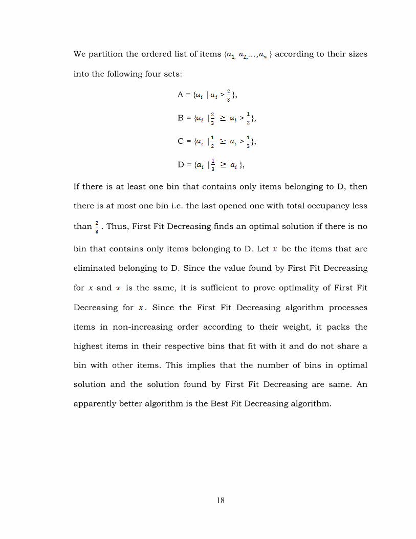
We partition the ordered list of items { …, } according to their sizes

into the following four sets:

A = { | > },

B = { | > },

C = { | > },

D = { | },

If there is at least one bin that contains only items belonging to D, then

there is at most one bin i.e. the last opened one with total occupancy less

than . Thus, First Fit Decreasing finds an optimal solution if there is no

bin that contains only items belonging to D. Let be the items that are

eliminated belonging to D. Since the value found by First Fit Decreasing

for x and is the same, it is sufficient to prove optimality of First Fit

Decreasing for . Since the First Fit Decreasing algorithm processes

items in non-increasing order according to their weight, it packs the

highest items in their respective bins that fit with it and do not share a

bin with other items. This implies that the number of bins in optimal

solution and the solution found by First Fit Decreasing are same. An

apparently better algorithm is the Best Fit Decreasing algorithm.

19

2.4.2 Best Fit Decreasing

Like First Fit Decreasing, Best Fit Decreasing initially sorts items in non-

increasing order with respect to their order and then processes them

sequentially. The difference between the two algorithms is the rule used

for choosing the bin in which new item is inserted while trying to

pack . Best Fit Decreasing chooses a bin with the minimum empty

space to be left after the item is packed into a bin. In this way, it tries to

fit the items into bin by reducing the fragmentation of the bins. In some

cases, the quality of solution found by Best Fit Decreasing may be worse

than the quality of solution found by First Fit Decreasing. In other cases

Best Fit Decreasing finds an optimal solution while First Fit Decreasing

returns a non- optimal solution.

Next we present three algorithms in which the number of sets in

the partition is minimized according to a set of given intervals.

2.5 Online algorithm based on partitioning:

Some types of algorithm are based on a non-uniform partitioning of

interval space (0,1] into M sub-intervals and will run is O(n) time. It is

known that no on-line algorithm can have an asymptotic worst case ratio

<1.53. The best on-line algorithm given by Lee and Lee and called

Harmonic has a worst-case ratio of 1.69. The performance ratio is better

than the Best-Fit when the item sizes are uniformly distributed.

20

2.5.1 Harmonic Algorithm:

We are given a list of items L= { , , … }, each with item sizes (0<

≤ 1). The interval (0, 1] is partitioned into harmonic sub intervals

= where M is a positive integer. Type 1 is a bin

that contains items whose sizes are in the range , type 2 is a bin

that contains items whose sizes are in the range , type M is a bin

that contains items whose sizes are in the range Each item is

classified according to the size, i.e., if the item size is in the interval

the item is called item or -bin. For 1 ≤ j < k, at most j -pieces can

be packed in –bin and is referred to as being filled if it has exactly –

pieces, and unfilled otherwise. Let denote the number of -bins used

by the algorithm, 1 ≤ j ≤ M. In Harmonic algorithm, we keep all unfilled

bins active -bin for each 1 ≤ j < M. The Harmonic algorithm is

completely independent of the arriving order of items [6].

All elements will be packed by Harmonic Fit into -bins as follows;

Items of type i are packed i per bin for i = 1, . . . ,k-1, and corresponding

weight is we classify the bins into M j- 1 categories. Each category is

designated to pack the same type of elements. It essentially performs

item classification for each incoming item and then packs it by Next Fit

into a corresponding bin. Now, items of type k are packed using Next Fit

21

When an item does not fit in a bin, the bin is at least full (size of each

item ≤ ) and the weight of item of size x is x. For the Next Fit, if the

next small element does not fit into the opened bin, we close this bin and

open a new bin. Elements of type k-1 pack k-1 per bin. The maximum

wasted space is maximal for type 1 bin, as they pack 1 per bin.

The Algorithm Harmonic has the following steps:

_______________________________________________________________________

Algorithm Harmonic ________________________________________________________________________ For a given value of N, M, and the set of items L= { , , … }

Step 1: Partition the interval (0, 1] for the given M into subintervals as

given below:

Step 2: Assign each item ai to the open bin of that type (the size of ai fits

into the corresponding subinterval).

Step 3: If an item does not fit into the corresponding bin, then close it

and open a new one.

Step 4: Calculate the total number of bins used of each type.

________________________________________________________________________

Let us consider an example where M=5 and the sequence of items is

0.21, 0.41, 0.13, 0.59, 0.75, 0.64, 0.75, 0.83, 0.71, 0.81, 0.2, 0.95, 0.37,

0.67, 0.44, 0.82, 0.21, 0.84, 0.87, 0.81, 0.79, 0.59, 0.87, 0.41, 0.25,

0.36, 0.25, 0.17, 0.29, 0.19, 0.8, 0.05, 0.63, 0.33, 0.56, 0.18, 0.79, 0.16,

22

0.13, and 0.19. Thus the interval (0, 1] is partitioned into five

subintervals are (0, ], ( , ], ( , ], ( , ], ( ,1]. Bins are assigned to each

interval as presented in the Table 1 for each partition. The total number

of bins used is 27.

Partition 1- (0, ]

Bin 1 0.13 0.2 0.17 0.19 0.15 0.18

Bin 2 0.16 0.13 0.19

Partition 2- ( , ]

Bin 1 0.21 0.21 0.25 0.25

Partition 3 - ( , ]

Bin1 0.29 0.23

Partition 4 - ( , ]

Bin 1 0.41 0.37

Bin 2 0.44 0.41

Bin 3 0.36

Partition 5 - ( , ]

Bins 1 2 3 4 5 6 7 8 9 10

Items 0.59 0.75 0.64 0.75 0.83 0.71 0.81 0.95 0.67 0.82

11 12 13 14 15 16 17 18 19 20 0.84 0.87 0.81 0.79 0.59 0.87 0.8 0.63 0.56 0.79

Table 1: Distribution of items using Harmonic algorithm

23

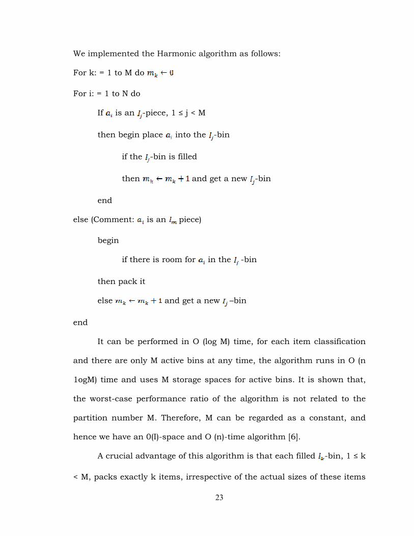
We implemented the Harmonic algorithm as follows:

For k: = 1 to M do

For i: = 1 to N do

If is an -piece, 1 ≤ j < M

then begin place into the -bin

if the -bin is filled

then and get a new -bin

end

else (Comment: is an piece)

begin

if there is room for in the -bin

then pack it

else and get a new –bin

end

It can be performed in O (log M) time, for each item classification

and there are only M active bins at any time, the algorithm runs in O (n

1ogM) time and uses M storage spaces for active bins. It is shown that,

the worst-case performance ratio of the algorithm is not related to the

partition number M. Therefore, M can be regarded as a constant, and

hence we have an 0(I)-space and O (n)-time algorithm [6].

A crucial advantage of this algorithm is that each filled -bin, 1 ≤ k

< M, packs exactly k items, irrespective of the actual sizes of these items

24

in the interval . A disadvantage of Harmonic is that items of type 1, that

is, the items larger than 1/2, are packed one per bin, possibly wasting a

lot of space in each single bin.

2.5.2 Epstein’s Algorithm:

We define bounded space algorithm of each value of m > 1. For every

m>1, changes on the lower bin are made. Epstein’s algorithm works the

same as the Harmonic algorithm except that in type M bins (the small

type bins), at most M items are stored at any time. Whenever M items are

stored in the small type bin, we close the bin and open a new one. For

item classification, we partition the interval (0, 1] into sub-intervals. We

use k–1 sub-intervals = . Each bin will contain

only items from one sub-interval (type). The items in interval are

packed to a single bin. A bin which received the full amount of items

(according to its type) is closed, therefore at most k − 1 bins are open

simultaneously (one per interval, except for ( ,1]. We pack each item

according to its type and we note again that the exact size does not affect

the packing process. Each bin will contain only items of one type. A bin

that has received the full amount of items (according to its type) is closed

[1]. The main difference between Harmonic algorithm and Epstein’s

algorithm is the way that small items are packed, no more than M items

are allowed in any bin, irrespective of whether more items can still fit

into that bin. The algorithm works as follows:

25

_______________________________________________________________________

Algorithm Epstein ________________________________________________________________________ For a given value of N, M, and the set of items L= { , , … }

Step 1: Partition the interval (0, 1] for the given M into subintervals:

Step 2: Assign each item ai to the open bin of that type (the size of ai fits

into the corresponding subinterval).

Step 3: If there are M items of type M into the small bin, then close it and

open a new one.

Step 4: If an item does not fit into the corresponding bin, then close it

and open a new one.

Step 5: Calculate the total number of bins used of each type.

________________________________________________________________________

Let us consider the following example, where M=5 and the sequence of

items is 0.21, 0.41, 0.13, 0.59, 0.75, 0.64, 0.75, 0.83, 0.71, 0.81, 0.2,

0.95, 0.37, 0.67, 0.44, 0.82, 0.21, 0.84, 0.87, 0.81, 0.79, 0.59, 0.87,

0.41, 0.25, 0.36, 0.25, 0.17, 0.29, 0.19, 0.8, 0.05, 0.63, 0.33, 0.56, 0.18,

0.79, 0.16, 0.13, and 0.19. The interval (0, 1] is partitioned into the

subintervals (0, ], ( , ], ( , ], ( , ], ( ,1]. Bins are assigned to each

interval as presented in Table 2 for each partition. The total number of

bins formed is 27.

26

Partition 1- (0, ]

Bin1 0.13 0.2 0.17 0.19 0.05

Bin2 0.18 0.16 0.13 0.19

Partition 2- ( , ]

Bin1 0.21 0.21 0.25 0.25

Partition 3 - ( , ]

Bin1 0.29 0.23

Partition 4 - ( , ]

Bin1 0.41 0.37

Bin2 0.44 0.41

Bin3 0.36

Partition 5 - ( , ]

Bins 1 2 3 4 5 6 7 8 9 10

Items 0.59 0.75 0.64 0.75 0.83 0.71 0.81 0.95 0.67 0.82

11 12 13 14 15 16 17 18 19 20

0.84 0.87 0.81 0.79 0.59 0.87 0.8 0.63 0.56 0.79

Table 2: Distribution of items using Epstein algorithm

The Variable Harmonic algorithm proposed by Epstein considers

the bins sizes to be < . . . = 1. The items are classified into intervals

whose right endpoint is a critical size.

27

CHAPTER 3

K-BINARY ALGORITHM

K-Binary is one of the simplest unsupervised learning algorithms to

group the bins according to the interval. To achieve this, the interval (0,1]

is partitioned into sub intervals as follows (0, 1]= ( ) where =

( , ( ( for k= 1, 2… n-1 where k is the

number of partitions.

For example, if k=3 then the interval (0,1] is partitioned into three

intervals ( , ( and ( . Each item is classified

according to its interval i.e., if the item size is in the interval then the

item is called an -item. Items in sub-interval k are packed to a bin. A

bin which received the full amount of items (according to its type) is

closed and therefore new bin is opened. Each bin will contain only items

from one sub-interval (type).

________________________________________________________________________

Algorithm k-Binary ________________________________________________________________________ For a given value of N, M, and the set of items L= { , , … }

Step 1: Partition the intervals for the given M value such that they are

partitioned into given intervals as given below.

( )

= ( , ( ( for k= 1,2… n-1

Step 2: Assign the items to bins according to each interval.

28

Step 3: Pack the items into each bin, if the next small element does not

fit into the opened bin, then we close this bin and open a new one.

Step 4: Calculate the total number of bins formed for each interval.

________________________________________________________________________

K- Binary algorithm mainly depends on three factors:

1) The number of items.

2) The number of partitions.

3) Bins that are assigned according to the given interval.

Let us consider the following example where M=5 and the items to

be packed are 0.2, 0.49, 0.85, 0.79, 0.53, 0.45, 0.31, 0.85, 0.56, 0.53,

0.85, 0.21, 0.1, 0.7, 0.76, 0.29, 0.54, 0.99, 0.31, 0.84, 0.8, 0.51, 0.15,

0.21, 0.47, 0.55, 0.69, 0.15, 0.44, 0.47, 0.15, 0.79, 0.9, 0.3, 0.24, 0.71,

0.46, 0.01, 0.69 and 0.16. The interval (0,1] is partitioned into five

subintervals (0, ], ( , ], ( , ], ( , ], ( ,1]. Bins are assigned to each

interval as presented in Table 3. The total number of bins formed is 29.

29

Partition 1- (0, ]

Bin 1 0.1

Partition 2- ( , ]

Bin 1 0.1

Partition 3 - ( , ]

Bin 1 0.2 0.21 0.15 0.21 0.15

Bin 2 0.15 0.24 0.16

Partition 4 - ( , ]

Bin 1 0.49 0.45

Bin 2 0.31 0.29 0.31

Bin 3 0.47 0.44

Bin 4 0.47 0.3

Bin 5 0.46

Partition 5 - ( , ]

Bins 1 2 3 4 5 6 7 8 9 10

Items 0.85 0.79 0.53 0.85 0.56 0.53 0.85 0.7 0.76 0.54

11 12 13 14 15 16 17 18 19 20

0.99 0.84 0.8 0.51 0.55 0.69 0.79 0.9 0.71 0.69

Table 3: Distribution of items using K- Binary algorithm

We implement the K- Binary algorithm as follows:

for i: = l to n do

begin

30

Case in

If is in –piece

Pack in empty bin of type

begin place into – bin

Pack in bins of type using the Best Fit algorithm

if there exists a nonempty bin of type that does not contain an -item

then pack in such a bin

else pack in an empty bin of type

If is the item to arrive, for some integer r≥ 1

then if there exists a bin of type containing at least one and at most

an -item

then pack in such a bin

else if there exists a bin of type containing only an -item

then pack in such a bin

else pack in an empty bin of type

else harmonic pack ( , )

end

It is obvious that each item takes O (1) time to pack. Therefore the

K- algorithm is an O (n) - time algorithm and it needs O (n) space [10].

The main goal using K-means algorithm is to minimize the number of

bins.

31

CHAPTER 4

IMPLEMENTATION AND COMPARISONS

In the thesis we implemented few methods in order to obtain the best

possible solution for any given sequence of requests and any value of M.

Different sequences of requests with different partitions produce different

results depending on size and data used. As the requests get large, the

number of bins generated by K-Binary algorithm compared to Harmonic

(Lee & Lee) does not give good results because of the size we have

chosen.

For generating random requests, instead of generating a random

integer i in the interval 1 to 10 and considering the size of the request to

be 1/random number, we generate requests of the type . Thus, if the

integers generated randomly are 5, 4, 7, 2, 5, 1 the data set becomes

. We compare the performance of the K-binary algorithm

with the performance of Harmonic (proposed by Lee and Lee) and we

obtained that in most of the cases, the K-Binary algorithm uses more

bins that Harmonic. Hence we measure the efficiency of the implemented

algorithms in a different way.

The algorithm begins with measuring the average number of bins

of any type used. For a given input, let N be the total number of items

and M be the total number of partitions. Consider TB1 to be the total

number of bins used by Harmonic (Lee & Lee), TB2 to be the total

32

number of bins used by Epstein and TB3 be the total number of bins

used by the K-Binary algorithm. For each algorithm we will compute how

well the algorithm balances the bins of any type. For an algorithm, let TB

be the total number of bins. The next step is to compute how many bins

of each type are used. Let NB1, NB2 ...NBM be the number of bins of type

1, type 2… type M used by the algorithm on that input. Now, if the

algorithm has a balanced distribution over the number of bins, then all

NBi should be roughly TB/M. For each input, after we compute the total

number of bins the next step is to compute the sum based on the below

formula:

(NB1 - TB/M)2 + (NB2 - TB/M)2 + (NB3 - TB/M)2 + ... (NBM - TB/M)2.

We will then average these numbers the same way we do with the

total number of bins.

4.1 Concrete Examples

We present some concrete examples that will include a sequence of

requests and the bins used by the k-Binary algorithm. We give an

example in which it shows that the k- Binary algorithm works better

than Epstein’s algorithm and equally well as Lee and Lee’s algorithm,

and another example showing that Lee and Lee performs better

compared to k- Binary algorithm. We also show how the proposed k-

Binary algorithm works. Let us consider examples where N random

requests will be fitted into M different types of bins. For N=100 and M=5,

33

in Table 4 we show how many bins of type 1 through 5 are used by each

algorithm.

Bins Lee & Lee Epstein K- Binary

NB_1 3 3 1

NB_2 2 2 1

NB_3 4 6 4

NB_4 10 11 14

NB_5 49 49 49

Total 68 71 69

Table 4: Example 1- comparison between Lee& Lee, Epstein & K-Binary

We compute the average sum for each algorithm as described before.

Average number of bins of Lee & Lee:

(3 - 68/5)2 + (3 - 68/5)2 + (4 - 68/5)2 + (10 – 68/5)2 + (49 - 68/5)2=23.61

Average number of bins of Epstein:

(3 - 71/5)2 + (2 - 68/5)2 + (6 - 68/5)2 + (11 – 68/5)2 + (49 - 68/5)2=22.10

Average number of bins of k-Binary:

(1 - 69/5)2 + (1 - 68/5)2 + (4 - 68/5)2 + (14 – 68/5)2 + (69 - 68/5)2=22.99

Therefore our proposed k-Binary algorithm performs better than

Lee and Lee’s and Epstein’s algorithms.

We take another example for same number of items and partitions.

We get different data set as items are generated randomly. For N=100

34

and M=3, in Table 5 we show what number of bins of each of the types 1

through 5 are used by each algorithm.

Bins Lee & Lee Epstein K- Binary

NB_1 2 4 1

NB_2 2 2 1

NB_3 3 3 2

NB_4 8 8 12

NB_5 49 49 49

Total 64 65 66

Table 5: Example 2- comparison between Lee& Lee, Epstein & K-Binary

Average sum obtained for Lee and Lee algorithm is 26.10, Epstein

algorithm is 24.97 and K- Binary algorithm is 25.40. Therefore as seen

from the two examples K- Binary algorithm performs better compared to

other two. Now we take another example and find the average for the

three algorithms for N=100 and M=5. Average obtained for Lee and Lee

algorithm is 26.55, Epstein algorithm is 25.21 and K- Binary algorithm is

27.71. Hence from the above example lee and lee performs better

compared to K- Binary algorithm.

35

Bins Lee & Lee Epstein K-Binary

NB_1 3 5 1

NB_2 2 2 1

NB_3 3 3 3

NB_4 7 7 10

NB_5 50 50 50

Total 65 67 65

Table 6: Example 3- Comparison between Lee& Lee, Epstein & K-Binary

4.2 Pre Processing:

Input File:

We generate random value for the requests and we store them in the file

input.dat. In the preprocessing step a set of N of items are obtained

randomly (called random sequence) , ,…, with in the range

0.01…0.99, to which we append another set of N values that are

computed as (1- random sequence) (called computed sequence).At the

beginning of the file we store the values of N and M, followed by the two

sequences.

Description:

Input the value N and M.

Start the random number generator.

Generate N rational values in the range 0.01 to 0.99 that will represent

36

the sequence of requests generated in the file "input.dat" first the value of

N, then M, then the sequence randomly generated

An example of such an input file is shown in Figure 7. where the

first number represents N i.e. total number of items generated randomly

and the second number M represents the number of partitions. Then we

have the random sequence followed by the computed sequence.

Figure 7: A Screenshot showing random number generation

37

4.3 Lee and Lee Algorithm:

Bins are packed according to the intervals described in Chapter 3.

Output: Display the number of bins needed and the content of the bins.

Description: Read from the file the value N, M and the sequence of

requests . Then compute the number of bins needed using the

algorithm of Lee and Lee. Finally display the results. Each time for

different input file and for different partitions the above steps are

performed and the number of bins are generated differently as shown in

Figure 8.

Figure 8: A Screenshot of output for Lee and Lee algorithm

38

For harmonic algorithm implemented by Lee and Lee and Epstein,

intervals and corresponding bin types are defined in the Table 7

Table 7: Intervals formed for Lee and Lee, Epstein

4.4 Epstein Algorithm:

In this algorithm, changes to the lowest indexed bin are made. For the

lowest indexed bin only at most k-items are assigned (as described in

Chapter 2).

Input: the file "input.dat"

Output: display the number of bins needed and the content of the bins

Description:

Read from the file the value N, M and the sequence of requests .

Then compute the number of bins needed using the algorithm of Epstein

and display the results. Therefore total number of bins obtained by the

algorithm is shown in the screenshot of Figure 9.

Interval Bin Type = (0, ]

= ( , ]

= ( , ]

= ( , ]

39

Figure 9: A Screenshot of output for Epstein algorithm

4.5 K- Binary Algorithm: In k-Binary algorithm bins are formed

according to the interval and the number of bins obtained by the

algorithm is shown in the screenshot of figure 10.

40

Figure 10: A Screenshot of output for K-binary

Intervals and corresponding bin type are defined in the interval below for

k-Binary algorithm.

41

Table 8: Intervals formed for K-binary algorithm

4.6 Algorithm Implementation:

It is implemented in java and randomly generated items generated are

stored in the file input.dat.

Below is a part of code for random generation of items

for (int i = 0;i<N;i++) { z = (int)Math.round(((double)Math.random()*1) * 100)/100.0; p.println(z); arr.add(z); } for(int i = 0;i<N;i++) p.println(Math.round((1 - arr.get(i))*100)/100.0); System.out.println("File Created"); } }

Then we create the partition of items as shown with a part of code below

and we name it as Abstract bin

public void createPartitions () { partition = new ArrayList [NumberOfPartitions];

Interval Bin Type = (0, ]

= ( , ]

= ( , ]

= ( , ]

42

for(int i = 0;i<NumberOfPartitions++) { partition[i] = new ArrayList<Bin>(1); partition[i].add(new Bin()); } } Once the partitions are created then we display the partition of items which is described in the code below if(!partition[PartitionNumber].get(0).toString().equals("")) for(int i = 0;i<partition[PartitionNumber].size();i++) { result += "Bin " + (i+1) +" - " + partition[PartitionNumber].get(i).toString() + "\n"; NumberOfBins++; } return result;} Once number of partitions is obtained then number of bins obtained by Lee and Lee is explained in the part of code below if(flag) { if(!partition[NumberOfPartitions - end].get(partition[NumberOfPartitions - end].size()-1).check(number)) partition[NumberOfPartitions - end].add(new Bin()); partition[NumberOfPartitions - end].get(partition[NumberOfPartitions - end].size()-1).addElement(number); partition[NumberOfPartitions - end].set(partition[NumberOfPartitions –v end].size()-1,partition[NumberOfPartitions -nd].get(partition[NumberOfPartitions - end].size()-1)); break; } start = end; end -= 1; } }

Then the items are assigned according to each interval is described in the

code below

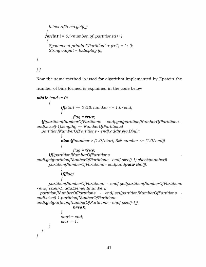
for(int i = 0;i<number_of_items;i++) {

43

b.insert(items.get(i)); } for(int i = 0;i<number_of_partitions;i++) { System.out.println ("Partition” + (i+1) + " : "); String output = b.display (i);

}

} }

Now the same method is used for algorithm implemented by Epstein the

number of bins formed is explained in the code below

while (end != 0) { if(start == 0 && number <= 1.0/end) { flag = true; if(partition[NumberOfPartitions - end].get(partition[NumberOfPartitions - end].size()-1).length() == NumberOfPartitions) partition[NumberOfPartitions - end].add(new Bin()); } else if(number > (1.0/start) && number <= (1.0/end)) { flag = true; if(!partition[NumberOfPartitions - end].get(partition[NumberOfPartitions - end].size()-1).check(number)) partition[NumberOfPartitions - end].add(new Bin()); } if(flag) { partition[NumberOfPartitions - end].get(partition[NumberOfPartitions - end].size()-1).addElement(number); partition[NumberOfPartitions - end].set(partition[NumberOfPartitions - end].size()-1,partition[NumberOfPartitions -end].get(partition[NumberOfPartitions - end].size()-1)); break; } start = end; end -= 1; } } }

44

Now for the K-Binary algorithm the number of bins obtained is described

in the code below

while(end != 0) { if(start == 0 && number <= 1.0/Math.pow(2,(end-1))) { flag = true; } else if(number > (1.0/Math.pow(2,(start-1))) && number <= 1.0/Math.pow(2,(end-1)))) { flag = true; } if(flag) { if(!partition[NumberOfPartitions - end].get(partition[NumberOfPartitions - end].size()-1).check(number)) partition [NumberOfPartitions - end].add(new Bin()); Partition [NumberOfPartitions - end].get(partition[NumberOfPartitions - end].size()-1).addElement(number); partition[NumberOfPartitions - end].set(partition[NumberOfPartitions - end].size()-1,partition[NumberOfPartitions - end].get(partition[NumberOfPartitions - end].size()-1)); break; } start = end; end -= 1; } } }

Thus, all these steps are implemented. The results obtained after

partitioning the intervals and analysis over the results for different

requests and graphs will be discussed in chapter 5 in the thesis.

45

CHAPTER 5

SIMULATION AND RESULTS

As discussed in Chapter 4, the K-Binary algorithm produces different

results for different set of items. This chapter is divided in two sections.

We first discuss the performance of the algorithm in terms of total

number of bins for different runs. In the second part we discuss the

performance of the algorithms based on the average values for the

number of bins of each type.

5.1 Comparison based on Bins:

We discuss the performance of the K- binary algorithm based on the total

number of bins. The bins formed vary for different algorithms. Table 9

provides the number of bins obtained for each algorithm according to the

items specified. From Table 9 we notice that if the items generated are 20

then the necessary number of bins is more than half the items. i.e. bins

formed are 13 for Lee and Lee, 14 for Epstein and K-binary results in 15,

and so on. There are some cases when our proposed K-Binary algorithm

requires less bins than Lee and Lee, and there are some cases where k-

Binary algorithm requires more bins than Lee and Lee. No trend has

been observed as for which number of items some algorithm is better.

46

Items LL E O

20 13 14 15

40 27 28 28

60 41 41 40

80 53 55 53

100 66 68 67

150 99 100 98

200 132 130 131

250 162 168 163

300 194 200 193

350 225 233 230

400 260 267 260

450 288 299 293

500 322 330 323

Table 9: Total bins formed for three algorithms for different items

5.2 Comparisons based on Average:

We compute the average based on bins formed for each algorithm when

the bins are separated into 5 partitions. We execute 50 different and we

compute the total number of bins by summing the number of bins of

each type as briefly described in Chapter 4. We also compute the average

of the bins among all types and we show the values in Table 10.

47

N Lee & Lee Epstein K-binary

20 5.017

4.0902 4.5152

40 9.5304 8.5226 8.8152

60 15.701 14.047 14.9744

80 20.756 19.0932 20.02

100 26.381 23.951 25.4988

150 40.0268 36.9672 38.9824

200 52.8476 49.39516 51.8582

250 66.8148 63.0702 65.9412

300 79.7872 75.40708 77.2372

350 93.5156 88.1338 92.3134

400 106.6986 102.793 107.5884

450 118.1946 112.2266 117.0962

500 132.7986 125.8654 131.5816

Table 10: Average values

Based on the average values from Table 10 of each algorithm we

draw two graphs. For the first graph we consider relatively smaller

number of items, for example 20, 40, 60, 80 and 100. The second graph

is drawn for large number of items. The x axis shows the number of bins

and the y axis show the average number of bins require by each

48

algorithm. We calculated the average with small or large sequences of

requests and random values for the requests.

Figure 11. Trend of AVG_OFFSET smaller number of items

From Figures 11 and 12 we draw the following observations:

In figure 11, we note that for smaller items there is not much variation

between the algorithms. The proposed K- Binary algorithm is as efficient

as Lee and Lee’s and Epstein’s algorithms. From Figure 12, we note that

for larger items the proposed K- Binary algorithm produces a lower

average than Lee and Lee but higher average than Epstein. We can then

conclude that the proposed K- binary algorithms behaves in average

better than both previously proposed algorithms in terms of the variance

49

on the type of bins used. Lee and Lee have a high variation on the type of

bins used, whereas Epstein uses more bins for packing the items than

Lee and Lee.

Figure 12. Trend of AVG_OFFSET large number of items

50

CHAPTER 6

CONCLUSION AND FUTURE WORK

Allocating memory in a data center for storage requests can be modeled

as a classical bin packing problem where online requests for storage are

served in minimum time and with the minimum cost. The cost for

hardware components if cheaper is the components are bought in bulk;

the maintenance is also easier. So we can assume that in a data center

all the hard disks have the same capacity. The goal of bin packing

problem is to minimize the number of bins used for serving a fixed

number of requests. The algorithm proposed by Lee and Lee has a

competitive ratio that is very close to the optimum, but has a high

variation on the types of bins used, in the sense that for random

requests it either uses a lot of small type bins or a lot of large type bins.

The algorithm proposed by Epstein has a worse competitive ratio, i.e.

uses more bins for packing the items than Lee and Lee, but it has a

much smaller variation than Lee and Lee. We propose an algorithm, K-

binary, that uses fewer bins than the algorithm proposed by Epstein, and

a slightly more bins than the algorithm proposed by Lee and Lee. At the

same time, the K-Binary algorithm works better than both previously

proposed algorithms. We drew these conclusions after executing

extensive simulations with small or large sequences of requests and

random values for the requests.

51

This thesis focuses on serving the requests using one dispatcher.

But modern computers have multiple processors, thus it is of future

interest to provide algorithms with better competitive ratio than Lee and

Lee that allow serving two or more requests at a time. For example, if two

requests can be served at the same time, we can have bins that can be

filled simultaneously by two dispatchers and allow only one dispatcher to

fill a bin in the moment the bin is close to be filled, for example, it needs

one more item to be filled.

52

BIBLIOGRAPHY

1. New Bounds for Variable-Sized Online Bin- Packing, Steven S. Seiden, Rob Van Stee, and Leah Epstein 2. D.J. Brown, A Lower Bound for On-Line One-Dimensional Bin Packing Algorithms, Tech.report R-864, Coordinated Science Laboratory, Urbana, IL, 1979. 3. E. G. Coffman, M. R. Garey, and D. S. Johnson, Approximation algorithms for bin packing: A survey, in Approximation Algorithms for NP-Hard Problems, D. Hochbaum, ed., PWS Publishing, Boston, 1997, Chap. 2. 4. J. Csirik, An on-line algorithm for variable-sized bin packing, Acta Inform., 26 (1989), pp.697–709. 5. N. Kinnersley and M. Langston, Online variable-sized bin packing, Discrete Appl. Math., 22 (1989), pp. 143–148. 6. C. Lee and D. Lee, A simple on-line bin-packing algorithm, J. ACM, 32 (1985), pp. 562–572. 7. F. M. Liang, A lower bound for online bin packing, Inform. Process. Lett. 10 (1980), pp. 76–79. 8. P. Ramanan, D. Brown, C. Lee, and D. Lee, On-line bin packing in linear time, J. Algorithms, 10 (1989), pp. 305–326. 9. Comparing Online Algorithms for Bin Packing Problems, Leah Epstein1, Lene M. Favrholdt2, and Jens S. Kohrt2, 1 Department of Mathematics, University of Haifa, Israel. 10. D.S. Johnson, A.Demers, J.D. Ullman, M.R. Garey, and R.L. Graham. Worst-case performance bounds for simple one-dimensional packing algorithms. SIAM Journal on Computing, 3(4):299{325, 1974. 11. C. Kenyon. Best- Fit bin-packing with random order. In Proceedings of the 7th Annual ACM-SIAM Symposium on Discrete Algorithms, pages 359{364, 1996. 12. E.G. Coffman, Jr.M.R. Garey, and D. S. Johnson Approximation algorithms for bin-packing: An updated survey. In G. Ausiello, M. Lucertini, and P. serafini, editors, Algorithm Design for Computer System Design, pages 49-106. Springer- Verlag, Wien, 1984. CISM Courses and Lectures Number 284.

53

13. J. Csirik, J. B. G. Frenk, A. Frieze, G. Galambos, and A. H. G. Rinnooy Kan. A probabilistic analysis of next fit decreasing bin packing heuristics. Oper. Res. Lett., 5:2333-236, 1986. 14. C.C. Lee, D.T Lee. A new algorithm for on-line bin packing. Tech. Rep. No. 83-03-FC- 02, Dept. of Electrical Engineering and Computer Science, Northwestern Univ., Evanston, Ill., Nov. 1983. 15. M. R. Carey, D.S. Johnson. Approximation algorithms for bin packing problems: A survey. In Analysis and Design of Algorithms in Combinatorial Optimization, G. Ausiello and M. Lucertini, Eds. Springer-Verlag, New York, 1981. 16. An Optimal Online Algorithm for Bounded Space Variable-Sized Bin Packing, Steven S. Seiden Department of Computer Science, 298 Coates Hall, Louisiana State University. 17. E.G. Coffman, M.R, Garey, D.S. Johnson. Approximation algorithms for bin packing: A survey. In Approximation Algorithms for NP-hard Problems, D. Hochbuam, Ed. PWS Publishing Company, 1997, ch. 2. 18. http://www.springerlink.com.ezproxy.library.unlv.edu/content/1w7 77ta6yp9rxa0c/fulltext.pdf 19. http://delivery.acm.org.ezproxy.library.unlv.edu/10.1145/10000/3 833/p562- lee.pdf? key1=3833&key2=2088707721&coll=ACM&dl=ACM& CFID=94375945&CFTOKEN=46821375 20. http://www.cs.ucsb.edu/~suri/cs130b/BinPacking.txt 21. http://delivery.acm.org.ezproxy.library.unlv.edu/10.1145/320000 /314083/p359- lenyon.pdf?key1=314083&key2=3778593721&coll=ACM &dl= ACM&CFID=90446320&CFTOKEN=36308439 22. http://www2.isye.gatech.edu/~mdrake/isye3103/BPPundergrad.pdf

54

VITA

Graduate College University of Nevada, Las Vegas

Swathi Venigella

Degrees: Bachelor of Engineering, Computer Science, 2008 JNTU University Master of Science, Computer Science, 2010 University of Nevada, Las Vegas Thesis Title: Cloud Storage and Online Bin Packing Thesis Examination Committee:

Chairperson, Dr. Wolfgang Bein, Ph.D. Committee Member, Dr. Thomas Nartker, Ph.D. Committee Member, Dr. Yoohwan Kim, Ph.D Graduate College Representative, Dr. Shahram Latifi, Ph.D