General rights Copyright and moral rights for the publications made accessible in the public portal are retained by the authors and/or other copyright owners and it is a condition of accessing publications that users recognise and abide by the legal requirements associated with these rights.

Users may download and print one copy of any publication from the public portal for the purpose of private study or research.

You may not further distribute the material or use it for any profit-making activity or commercial gain

You may freely distribute the URL identifying the publication in the public portal If you believe that this document breaches copyright please contact us providing details, and we will remove access to the work immediately and investigate your claim.

Downloaded from orbit.dtu.dk on: Jan 12, 2020

The load-balanced multi-dimensional bin-packing problem

Trivella, Alessio; Pisinger, David

Published in:Computers & Operations Research

Link to article, DOI:10.1016/j.cor.2016.04.020

Publication date:2016

Document VersionPeer reviewed version

Link back to DTU Orbit

Citation (APA):Trivella, A., & Pisinger, D. (2016). The load-balanced multi-dimensional bin-packing problem. Computers &Operations Research, 74, 152-164. https://doi.org/10.1016/j.cor.2016.04.020

The load-balanced multi-dimensional bin-packingproblem

Alessio Trivellaa,∗, David Pisingera

aDepartment of Management Engineering, Technical University of Denmark,Produktionstorvet, Building 426, DK-2800 Kgs. Lyngby, Denmark

Abstract

The bin-packing problem is one of the most investigated and applicable combi-

natorial optimization problems. In this paper we consider its multi-dimensional

version with the practical extension of load balancing, i.e. to find the packing

requiring the minimum number of bins while ensuring that the average center of

mass of the loaded bins falls as close as possible to an ideal point, for instance

the center of the bin. We formally describe the problem using mixed-integer

linear programming models, from the simple case where we want to optimally

balance a set of items already assigned to a single bin, to the general balanced

bin-packing problem. Given the difficulty for standard solvers to deal even with

small size instances, a multi-level local search heuristic is presented. The algo-

rithm takes advantage of the Fekete-Schepers representation of feasible packings

in terms of particular classes of interval graphs, and iteratively improves the load

balancing of a bin-packing solution using different search levels. The first level

explores the space of transitive orientations of the complement graphs associ-

ated with the packing, the second modifies the structure itself of the interval

graphs, the third exchanges items between bins repacking proper n-tuples of

weakly balanced bins. Computational experiments show very promising results

on a set of 3D bin-packing instances from the literature.

Keywords: multi-dimensional bin-packing, load balancing, MILP modeling,

∗Corresponding authorEmail addresses: atri@dtu.dk (Alessio Trivella), dapi@dtu.dk (David Pisinger)

local search

1. Introduction

The bin-packing problem is one of the most investigated and applicable mod-

els in combinatorial optimization. The problem consists of packing objects of

different sizes into a finite number of similar bins/containers, in a way that the

number of used bins is minimized. The bin-packing problem can be seen as a5

special case of the cutting stock problem, in which each item has also a demand,

i.e. it must appear a specific number of times in the bins. There exist prac-

tical applications of the bin-packing problem in a broad range of disciplines,

such as transportation and logistics, computer science, engineering, economics

and manufacturing. For the variety and importance of its applications, the bin-10

packing problem has been intensively studied and several interesting ideas for

solving it have arisen during the years.

In some real-life situations, mostly related to the two- and three-dimensional

cases, we are not only interested in determining a packing with fewest bins,

but also obtaining well-balanced packings. Consider for example the problem15

of arranging items into an aircraft cargo area such that the center of mass, or

barycenter, of the loaded plane falls as close as possible to an ideal point given

by the aircraft’s specifications. The position of the barycenter has an impact

on the flight performance in terms of safety and efficiency, and even a minor

displacement from the ideal barycenter can lead to a high increase of fuel con-20

sumption [1]. Similar considerations apply in the loading of trucks and container

ships.

Packing and balancing a set of items represent two conflicting objectives and in

this paper we will investigate how to integrate them into a single problem. The

goal is to arrange the items in the smallest number of bins, while ensuring the25

best overall load balancing of the used bins.

2

1.1. Related Literature

In the following we present the essential literature along two main lines: the

classical multi-dimensional bin-packing problem and variants based on load bal-

ancing.30

The literature about multi-dimensional bin-packing is vast and a huge number

of heuristic algorithms and dedicated exact procedures have been developed.

Martello and Vigo [2] proposed the first exact method for the 2D bin-packing

problem using a two-level Branch-and-Bound method. Using a similar proce-

dure, Martello et al. [3] described an exact algorithm for the 3D case and35

introduced the discrete set of Corner Points to reduce the search space.

Fekete and Schepers [4, 5] defined an implicit representation of multi-dimensional

packings by means of interval graphs, built by checking whether the projections

of items on the coordinate axes are pairwise overlapping. With such character-

ization the authors successfully developed a two-level search tree.40

Several promising heuristics are based on a local search framework. Lodi et al.

[6] proposed a unified tabu search, called TSpack, which can be used for solving

many variants of any multi-dimensional bin-packing problem. Faroe et al. [7]

presented the Guided Local Search method where memory guides the search to

promising regions of the solution space.45

Crainic et al. [8] developed constructive heuristics based on an efficient way to

place items into a bin, exploiting the free volume better than previous meth-

ods. This is done introducing the Extreme Points, which extend the concept of

Corner Points. The same authors presented the TS 2pack [9], a two-level tabu

search algorithm which, among others, makes use of the graph representation of50

Fekete and Schepers to verify the feasibility of a packing and developed GASP

[10], a meta-heuristic framework for solving the multi-dimensional bin-packing

which combines the simplicity of greedy algorithms with learning mechanisms.

Other heuristic approaches for multi-dimensional bin-packing problems can be

found in Egeblad and Pisinger [11], Lodi et al. [12], Pisinger and Sigurd [13].55

In recent years some authors started to examine different packing-related prob-

lems involving the load balancing of items. The literature is however still quite

3

scarce, perhaps due to the fact that considering the load balancing adds further

complexity to the already NP-hard packing problems.

Davies and Bischoff [14] and Junqueira et al. [15] considered load balancing in60

the 3D container loading problem. Paquay et al. [16] provided a formulation of

3D bin-packing deriving from an air cargo application which takes into account

weight distribution constraints. Mongeau, Bes [1] and Kaluzny and Shaw [17]

also focused on the optimal aircraft load balancing. In papers [1, 14, 15, 16, 17]

the target is balancing a single bin and specific physical constraints related to65

for example aircraft’s specifications are included in the models.

In some papers the load balancing is handled by imposing the center of mass

to lie inside “stable” region. Baldi et al. [18] analyze a 3D knapsack problem

with these kinds of balancing constraints, whereas de Queiroz and Miyazawa

[19] consider the 2D strip packing.70

Using the concept of a stable region for a bin-packing problem imposes some

challenges. It may happen that no bin-packing solution using the smallest num-

ber of bins respects the balancing constraints, especially if the safe region is

very restricted. On the other hand, large regions allow a feasible barycenter too

far away from an ideal point, and in industrial situations it translates into an75

increase of costs or fuel consumption. Even though a stable region is relatively

easy to model, we will also investigate other ways of modeling the balance con-

straints.

Some authors model the load balancing with a multi-objective formulation

aimed to simultaneously minimize the number of used bins and the load im-80

balance of the bins, frequently solved using meta-heuristics. In particular, the

2D multi-objective bin-packing is solved by Fernandez et al. [20] using a paral-

lel memetic algorithm, and by Liu et al. [21] with evolutionary particle swarm

optimization. Imai et al. [22] consider the load balancing and stability factors

for a shipping cargo with a particular cellular structure to place containers.85

4

1.2. Recalling the bin-packing problem

The multi-dimensional bin-packing problem (MBP) can be formulated using a

mixed-integer linear programming (MILP) model. Assume a set of n rectangular-

shaped boxes indexed over V = 1, . . . , n is given in a D-dimensional space,

D ∈ N, and box i has sizes wid for d ∈ D. Infinitely many bins are available,

having identical sizes Wd. The goal is to orthogonally pack all boxes into the

bins avoiding overlap and using as few bins as possible. Rotation of items is not

allowed.

For each i ∈ V , d ∈ D, the variable xid ∈ R represents the coordinate of the

lower face of item i in direction d, while the lower face of the bins is assumed to

have coordinate 0 in every direction. The integer variable ai denotes the number

of the bin containing item i. Then, for each couple of items i, j ∈ V and d ∈ D,

we introduce the binary variable lijd = 1 if and only if box i is located entirely

lower than j in direction d. Let N denote the number of used bins, and lastly

consider the binary variables pij = 1 if and only if ai < aj . Thus, we can write

the following model:

min N (1)

s.t. :∑d∈D

(lijd + ljid) + pij + pji ≥ 1 ∀ i < j ∈ V (2)

xid − xjd +Wd lijd ≤Wd − wid ∀ i 6= j ∈ V, d ∈ D (3)

xid ≤Wd − wid ∀ i ∈ V, d ∈ D (4)

ai − aj + n pij ≤ n− 1 ∀ i 6= j ∈ V (5)

1 ≤ ai ≤ N ∀ i ∈ V (6)

var : aj , N ∈ N, xid ∈ R+, lijd, pij ∈ 0, 1 ∀ i, j ∈ V, d ∈ D (7)

Constraints (2) ensure that a pair of items i, j in the same bin do not overlap,

(3) translates the definition of lijd in a mathematical form, (4) ensures that the

bin’s boundaries are not exceeded and (5) forces two overlapping items to lie in

different bins.90

The model would remain correct with D = 1, but much simpler formulations

5

exist in such case and we will limit our discussion to D ≥ 2. Having a D-

dimensional formulation of the problem makes it easy for us to treat the two-

and three-dimensional cases simultaneously. Practical applications of the prob-

lem for more than three dimensions are more hypothetic, but Garey et al. [23]95

showed that many scheduling problems can be formulated as multi-dimensional

bin packing problems.

Notice that the model makes use of a large number of big-M constraints which

will loose their effect when solving the LP-relaxation, and thus bounds from the

LP-relaxation are generally far from the integer optimal solution value. More-100

over, the model contains many symmetric solutions, for example taking any

permutation of the bins ai. Constraints (5) have similarities with the Miller-

Tucker-Zemlin constraints for the Traveling Salesman Problem [24] and the ai

could be declared as real variables instead of integer but, because of the sym-

metry, without improving performance in a major way. For these reasons, even105

if we break some symmetries adding constraints as ai ≤ i, the model remains

extremely difficult to solve in practice for standard MILP solvers, frequently

failing even when dealing with instances constituting 30-35 items.

We have now all the elements to introduce the additional balancing requirement

and describe the load-balanced multi-dimensional bin-packing problem. The re-110

mainder of the paper is structured as follows. In Section 2 we formulate a MILP

model for the load-balanced multi-dimensional bin-packing problem. In Section

3 the exact theory is supported with the definition of a multi-level local search

heuristic algorithm able to handle also large instances. Section 4 is dedicated

to computational results and in Section 5 some conclusions are drawn.115

2. Modeling the load-balanced multi-dimensional bin-packing prob-

lem

The load-balanced multi-dimensional bin-packing problem consists in packing

parallelepiped objects into the smallest number of bins, in such a way that the

center of mass of the loaded bins fall as close as possible to a desired location.120

6

In other words, the sum of displacements from the desired barycenter location

over the (smallest number of) used bins is minimized.

To the best of our knowledge, no MILP model for such problem has been defined

in the literature, thus, we will treat it in details. The explanation simplifies if

we first consider the restricted problem where a single bin has to be balanced,125

and then extend to the general case.

2.1. Balancing a single bin

Suppose you have already obtained a feasible solution of the MBP using an

exact or heuristic method, and consider a single bin. We want to arrange a

set of m given boxes U = 1, 2, . . . ,m into the D-dimensional bin, so that the

distance between the barycenter of the loaded bin and our ideal point inside the

bin, for instance its geometrical center, is minimized. By assumption, the bin

can accommodate all the items.

Assume that boxes are homogeneous and have densities ρi, i ∈ U . With ρi we

can determine the mass mi of box i by mi = ρi · voli , where voli =∏

d∈D wid

is the volume of box i. Equivalently, we could be given directly the masses mi

instead of densities.

Concepts from physics, like density, mass and volume, normally refer to three-

dimensional objects, but will be abstractly used also in spaces of higher dimen-

sion.

Since box i is homogeneous and rectangular-shaped, its barycenter coincides

with its geometric center that corresponds to Ci = (xid + wid/2)d∈D, and the

barycenter B of the whole loaded bin can be computed using the expression:

B = (Bd)d∈D =

∑i∈U mi Ci∑i∈U mi

Then, the objective function f(x) = f((xid)i,d) represents the distance of the

barycenter B from its ideal location, denoted as Bopt = (Boptd )d∈D. The L1-

norm, or rectangular norm, i.e. the sum of the absolute values of the differences

in the D components, is used to compute the distance:

f(x) =∥∥Bopt −B

∥∥1

=∑d∈D

∣∣Boptd −Bd

∣∣7

The L1-norm is chosen since it better allows to separately manage the displace-

ments in each direction and because it can be easily linearized.

Sometimes it can be more important to balance in one coordinate than the oth-

ers. For example, someone might consider more relevant to obtain a perfect

balancing on the x and y axes of a 3D container without caring too much about

the height of the barycenter, or vice versa. As a consequence, some weights

kd ≥ 0 are incorporated into the definition of f in order to suit the individual

needs to tune the balancing criteria, and a more general objective function looks

like:

f(x) =∑d∈D

kd∣∣Bopt

d −Bd

∣∣As an example, when loading a truck, it could be reasonable to choose the

center of the base of the container as the ideal barycenter, i.e. the point with

coordinates ( 12 Wx,

12 Wy, 0). If we assume that a low barycenter is twice as

important as balancing in x and y directions, then the objective function will

look like | 12 Wx −Bx|+ | 12 Wy −By|+ 2|Bz|.

Coming back to the general case and substituting the components of B with

their full expressions, we obtain:

f(x) =∑d∈D

kd

∣∣∣∣∣Boptd − 1

MU

(∑i∈U

mi

(xid +

wid

2

))∣∣∣∣∣where MU =

∑i∈U mi is the total mass of boxes belonging to the set U .

The function f is not linear since it contains absolute values. A well-known

trick to handle an absolute value in the objective function is to introduce two

additional positive support variables indicating the positive and negative parts

of the quantity inside the absolute value. In our case we define rd, sd ≥ 0 for

d ∈ D satisfying:

rd − sd = Boptd − 1

MU

(∑i∈U

mi

(xid +

wid

2

))

making it possible to rewrite the objective to:

f(x) =∑d∈D

kd (rd + sd)

8

Finally, reusing the set of variables lijd already introduced for the MBP and the

blocks of constraints ensuring no overlap and no violation of the boundaries,

the problem is formulated using the following linear model:

min∑d∈D

kd (rd + sd) (8)

s.t. : rd − sd = Boptd − 1

MU

(∑i∈U

mi

(xid +

wid

2

))∀ d ∈ D

(9)∑d∈D

(lijd + ljid) ≥ 1 ∀ i < j ∈ U (10)

xid − xjd +Wd lijd ≤Wd − wid ∀ i 6= j ∈ U, d ∈ D (11)

xid ≤Wd − wid ∀ i ∈ U, d ∈ D (12)

var : xid, rd, sd ∈ R+ lijd ∈ 0, 1 ∀ i, j ∈ V, d ∈ D (13)

We will refer to (8-13) as the multi-dimensional single load-balancing problem

(SLB).

The structure is similar to the general MBP and most of the constraints are130

essentially the same. Hence, again, the large use of conditional constraints and

big-M coefficients makes it difficult to solve the model in practice using standard

solvers.

Notice that, by assumption, we start with a set of items which can be packed

into one container, hence feasible solutions do exist. However, this information135

is not present a priori in the model, and if the number of boxes is large (more

than 25-30) with a high filling of the bin’s volume, then it can be hard for the

solver even to find a feasible solution. Moreover, even when a feasible solution

is found quickly, the gap from the best lower bound can take a huge amount of

time to be closed.140

2.2. Packing and balancing

Moving forward to the general problem, we can first assign items to the minimum

number of bins by solving the MBP model, and next apply the SLB model to

9

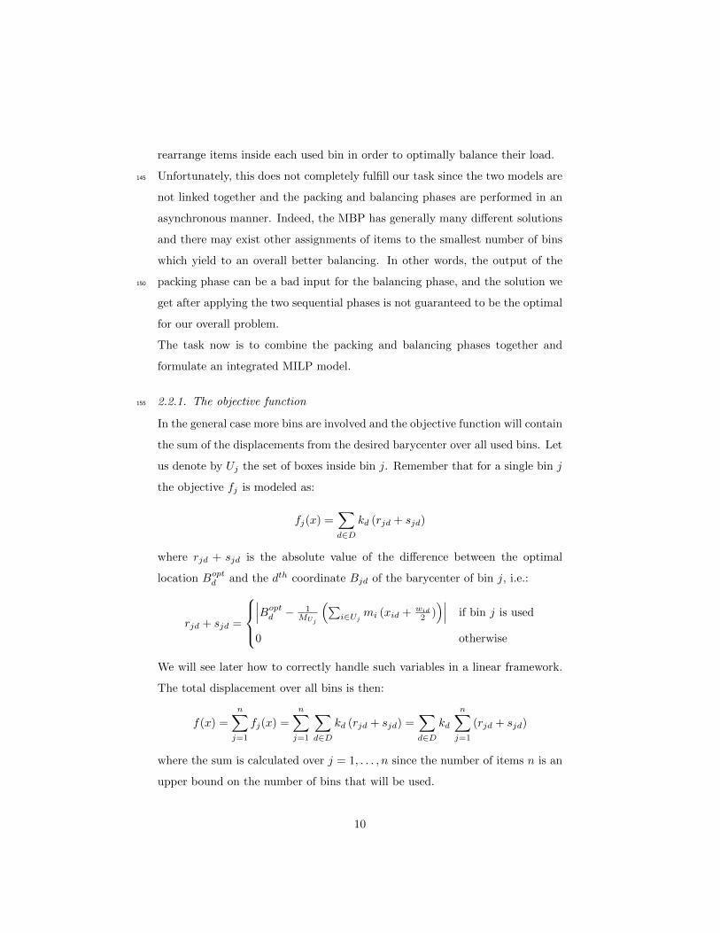
rearrange items inside each used bin in order to optimally balance their load.

Unfortunately, this does not completely fulfill our task since the two models are145

not linked together and the packing and balancing phases are performed in an

asynchronous manner. Indeed, the MBP has generally many different solutions

and there may exist other assignments of items to the smallest number of bins

which yield to an overall better balancing. In other words, the output of the

packing phase can be a bad input for the balancing phase, and the solution we150

get after applying the two sequential phases is not guaranteed to be the optimal

for our overall problem.

The task now is to combine the packing and balancing phases together and

formulate an integrated MILP model.

2.2.1. The objective function155

In the general case more bins are involved and the objective function will contain

the sum of the displacements from the desired barycenter over all used bins. Let

us denote by Uj the set of boxes inside bin j. Remember that for a single bin j

the objective fj is modeled as:

fj(x) =∑d∈D

kd (rjd + sjd)

where rjd + sjd is the absolute value of the difference between the optimal

location Boptd and the dth coordinate Bjd of the barycenter of bin j, i.e.:

rjd + sjd =

∣∣∣Bopt

d − 1MUj

(∑i∈Uj

mi (xid + wid

2 ))∣∣∣ if bin j is used

0 otherwise

We will see later how to correctly handle such variables in a linear framework.

The total displacement over all bins is then:

f(x) =

n∑j=1

fj(x) =

n∑j=1

∑d∈D

kd (rjd + sjd) =∑d∈D

kd

n∑j=1

(rjd + sjd)

where the sum is calculated over j = 1, . . . , n since the number of items n is an

upper bound on the number of bins that will be used.

10

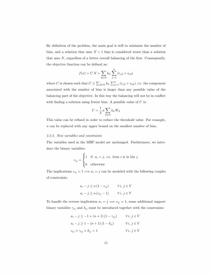
By definition of the problem, the main goal is still to minimize the number of

bins, and a solution that uses N + 1 bins is considered worse than a solution

that uses N , regardless of a better overall balancing of the first. Consequently,

the objective function can be defined as:

f(x) = C N +∑d∈D

kd

n∑j=1

(rjd + sjd)

where C is chosen such that C ≥∑

d∈D kd∑n

j=1 (rjd + sjd), i.e. the component

associated with the number of bins is larger than any possible value of the

balancing part of the objective. In this way the balancing will not be in conflict

with finding a solution using fewest bins. A possible value of C is:

C =1

2n∑d∈D

kdWd

This value can be refined in order to reduce the threshold value. For example,

n can be replaced with any upper bound on the smallest number of bins.

2.2.2. New variables and constraints

The variables used in the MBP model are unchanged. Furthermore, we intro-

duce the binary variables:

cij =

1 if ai = j, i.e. item i is in bin j

0 otherwise

The implications cij = 1 =⇒ ai = j can be modeled with the following couples

of constraints:

ai − j ≤ n (1− cij) ∀ i, j ∈ V

ai − j ≥ n (cij − 1) ∀ i, j ∈ V

To handle the reverse implication ai = j =⇒ cij = 1, some additional support

binary variables γij and δij must be introduced together with the constraints:

ai − j ≤ −1 + (n+ 1) (1− γij) ∀ i, j ∈ V

ai − j ≥ 1− (n+ 1) (1− δij) ∀ i, j ∈ V

cij + γij + δij = 1 ∀ i, j ∈ V

11

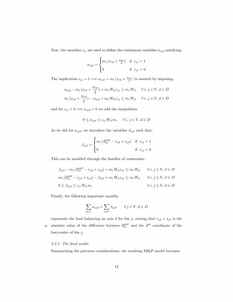
Now, the variables cij are used to define the continuous variables αijd satisfying:

αijd =

mi (xid + wid

2 ) if cij = 1

0 if cij = 0

The implication cij = 1 =⇒ αijd = mi (xid + wid

2 ) is ensured by imposing:

αijd −mi (xid +wid

2) +miWd cij ≤ miWd ∀ i, j ∈ V, d ∈ D

mi (xid +wid

2)− αijd +miWd cij ≤ miWd ∀ i, j ∈ V, d ∈ D

and for cij = 0 =⇒ αijd = 0 we add the inequalities:

0 ≤ αijd ≤ cij Wdmi ∀ i, j ∈ V, d ∈ D

As we did for αijd, we introduce the variables βijd such that:

βijd =

mi (Boptd − rjd + sjd) if cij = 1

0 if cij = 0

This can be modeled through the families of constraints:

βijd −mi (Boptd − rjd + sjd) +miWd cij ≤ miWd ∀ i, j ∈ V, d ∈ D

mi (Boptd − rjd + sjd)− βijd +miWd cij ≤ miWd ∀ i, j ∈ V, d ∈ D

0 ≤ βijd ≤ cij Wdmi ∀ i, j ∈ V, d ∈ D

Finally, the following important equality∑i∈V

αijd =∑i∈V

βijd ∀ j ∈ V, d ∈ D

represents the load balancing on axis d for bin j, stating that rjd + sjd is the

absolute value of the difference between Boptd and the dth coordinate of the160

barycenter of bin j.

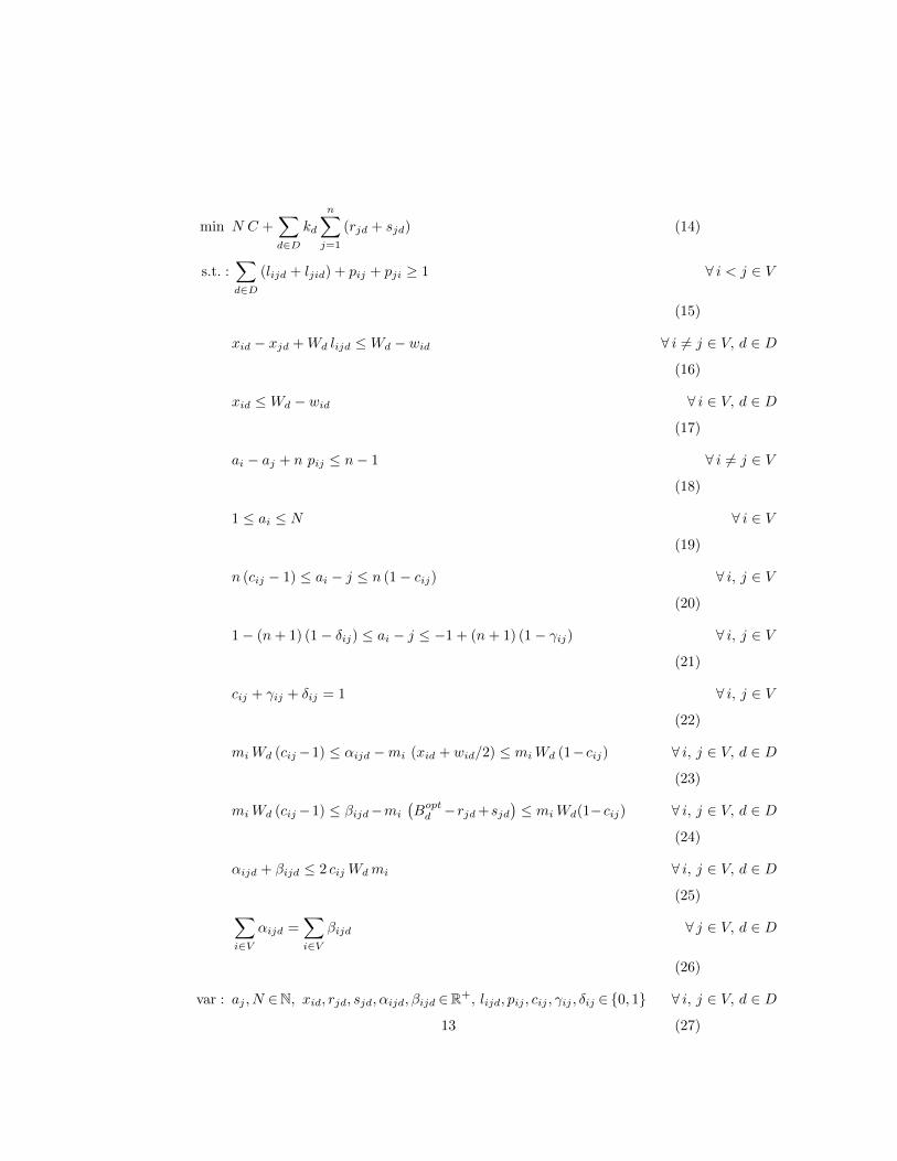
2.2.3. The final model

Summarizing the previous considerations, the resulting MILP model becomes

12

min N C +∑d∈D

kd

n∑j=1

(rjd + sjd) (14)

s.t. :∑d∈D

(lijd + ljid) + pij + pji ≥ 1 ∀ i < j ∈ V

(15)

xid − xjd +Wd lijd ≤Wd − wid ∀ i 6= j ∈ V, d ∈ D

(16)

xid ≤Wd − wid ∀ i ∈ V, d ∈ D

(17)

ai − aj + n pij ≤ n− 1 ∀ i 6= j ∈ V

(18)

1 ≤ ai ≤ N ∀ i ∈ V

(19)

n (cij − 1) ≤ ai − j ≤ n (1− cij) ∀ i, j ∈ V

(20)

1− (n+ 1) (1− δij) ≤ ai − j ≤ −1 + (n+ 1) (1− γij) ∀ i, j ∈ V

(21)

cij + γij + δij = 1 ∀ i, j ∈ V

(22)

miWd (cij−1) ≤ αijd −mi (xid + wid/2) ≤ miWd (1−cij) ∀ i, j ∈ V, d ∈ D

(23)

miWd (cij−1) ≤ βijd−mi

(Bopt

d −rjd +sjd)≤ miWd(1−cij) ∀ i, j ∈ V, d ∈ D

(24)

αijd + βijd ≤ 2 cij Wdmi ∀ i, j ∈ V, d ∈ D

(25)∑i∈V

αijd =∑i∈V

βijd ∀ j ∈ V, d ∈ D

(26)

var : aj , N ∈N, xid, rjd, sjd, αijd, βijd ∈R+, lijd, pij , cij , γij , δij ∈ 0, 1 ∀ i, j ∈ V, d ∈ D

(27)13

In the following we refer to (14-27) as LB-MBP.

The number of variables and constraints is greatly increased, although remaining165

O(n2). In practice, this model is extremely difficult to solve even for small

instances with 20-25 items.

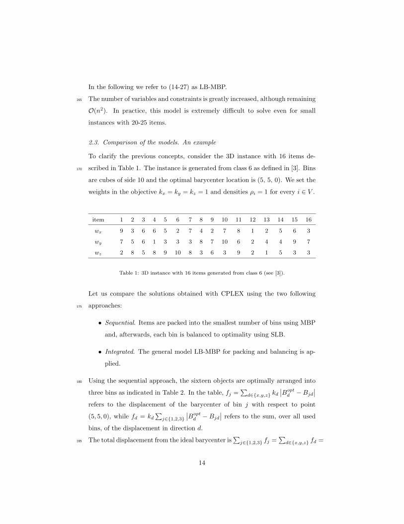
2.3. Comparison of the models. An example

To clarify the previous concepts, consider the 3D instance with 16 items de-

scribed in Table 1. The instance is generated from class 6 as defined in [3]. Bins170

are cubes of side 10 and the optimal barycenter location is (5, 5, 0). We set the

weights in the objective kx = ky = kz = 1 and densities ρi = 1 for every i ∈ V .

item 1 2 3 4 5 6 7 8 9 10 11 12 13 14 15 16

wx 9 3 6 6 5 2 7 4 2 7 8 1 2 5 6 3

wy 7 5 6 1 3 3 3 8 7 10 6 2 4 4 9 7

wz 2 8 5 8 9 10 8 3 6 3 9 2 1 5 3 3

Table 1: 3D instance with 16 items generated from class 6 (see [3]).

Let us compare the solutions obtained with CPLEX using the two following

approaches:175

• Sequential. Items are packed into the smallest number of bins using MBP

and, afterwards, each bin is balanced to optimality using SLB.

• Integrated. The general model LB-MBP for packing and balancing is ap-

plied.

Using the sequential approach, the sixteen objects are optimally arranged into180

three bins as indicated in Table 2. In the table, fj =∑

d∈x,y,z kd∣∣Bopt

d −Bjd

∣∣refers to the displacement of the barycenter of bin j with respect to point

(5, 5, 0), while fd = kd∑

j∈1,2,3∣∣Bopt

d −Bjd

∣∣ refers to the sum, over all used

bins, of the displacement in direction d.

The total displacement from the ideal barycenter is∑

j∈1,2,3 fj =∑

d∈x,y,z fd =185

14

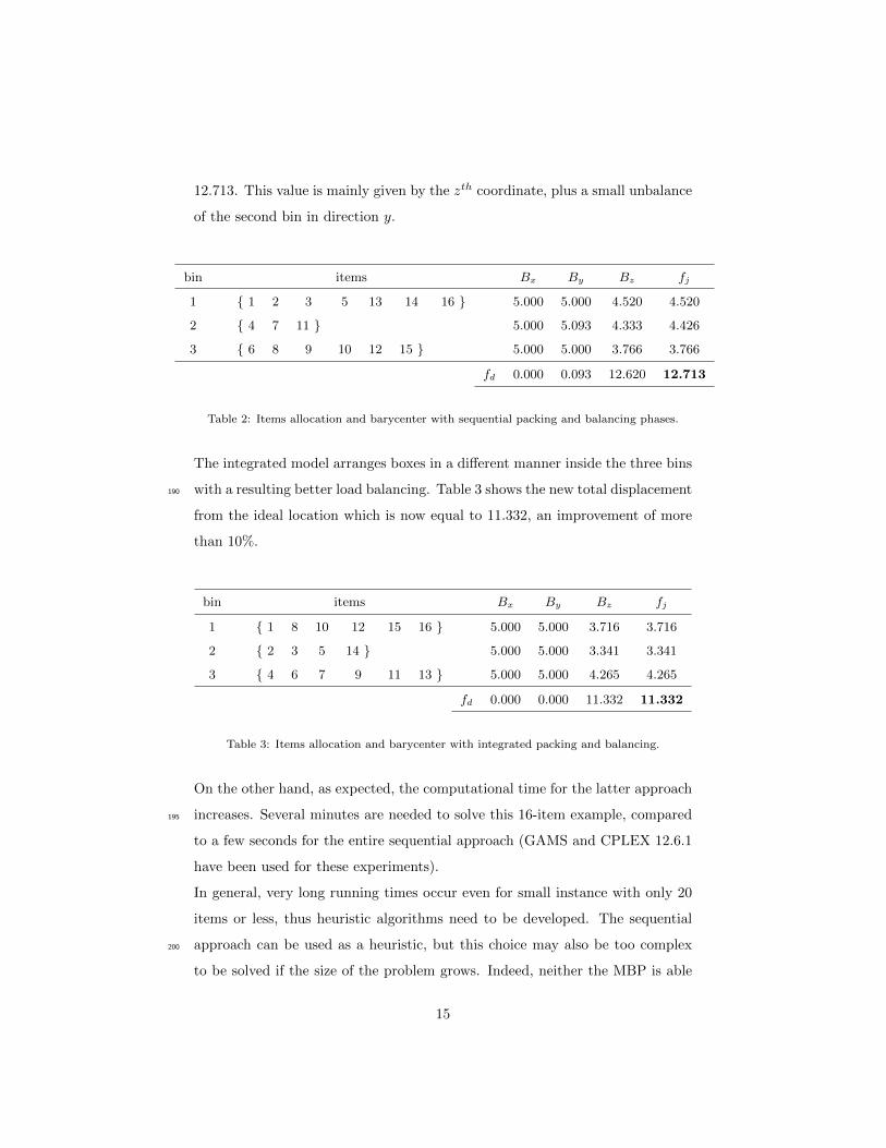
12.713. This value is mainly given by the zth coordinate, plus a small unbalance

of the second bin in direction y.

bin items Bx By Bz fj

1 1 2 3 5 13 14 16 5.000 5.000 4.520 4.520

2 4 7 11 5.000 5.093 4.333 4.426

3 6 8 9 10 12 15 5.000 5.000 3.766 3.766

fd 0.000 0.093 12.620 12.713

Table 2: Items allocation and barycenter with sequential packing and balancing phases.

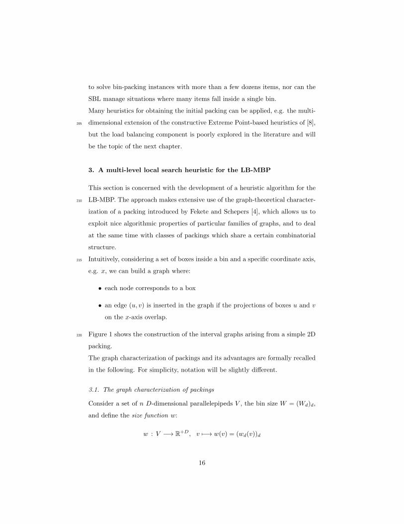
The integrated model arranges boxes in a different manner inside the three bins

with a resulting better load balancing. Table 3 shows the new total displacement190

from the ideal location which is now equal to 11.332, an improvement of more

than 10%.

bin items Bx By Bz fj

1 1 8 10 12 15 16 5.000 5.000 3.716 3.716

2 2 3 5 14 5.000 5.000 3.341 3.341

3 4 6 7 9 11 13 5.000 5.000 4.265 4.265

fd 0.000 0.000 11.332 11.332

Table 3: Items allocation and barycenter with integrated packing and balancing.

On the other hand, as expected, the computational time for the latter approach

increases. Several minutes are needed to solve this 16-item example, compared195

to a few seconds for the entire sequential approach (GAMS and CPLEX 12.6.1

have been used for these experiments).

In general, very long running times occur even for small instance with only 20

items or less, thus heuristic algorithms need to be developed. The sequential

approach can be used as a heuristic, but this choice may also be too complex200

to be solved if the size of the problem grows. Indeed, neither the MBP is able

15

to solve bin-packing instances with more than a few dozens items, nor can the

SBL manage situations where many items fall inside a single bin.

Many heuristics for obtaining the initial packing can be applied, e.g. the multi-

dimensional extension of the constructive Extreme Point-based heuristics of [8],205

but the load balancing component is poorly explored in the literature and will

be the topic of the next chapter.

3. A multi-level local search heuristic for the LB-MBP

This section is concerned with the development of a heuristic algorithm for the

LB-MBP. The approach makes extensive use of the graph-theoretical character-210

ization of a packing introduced by Fekete and Schepers [4], which allows us to

exploit nice algorithmic properties of particular families of graphs, and to deal

at the same time with classes of packings which share a certain combinatorial

structure.

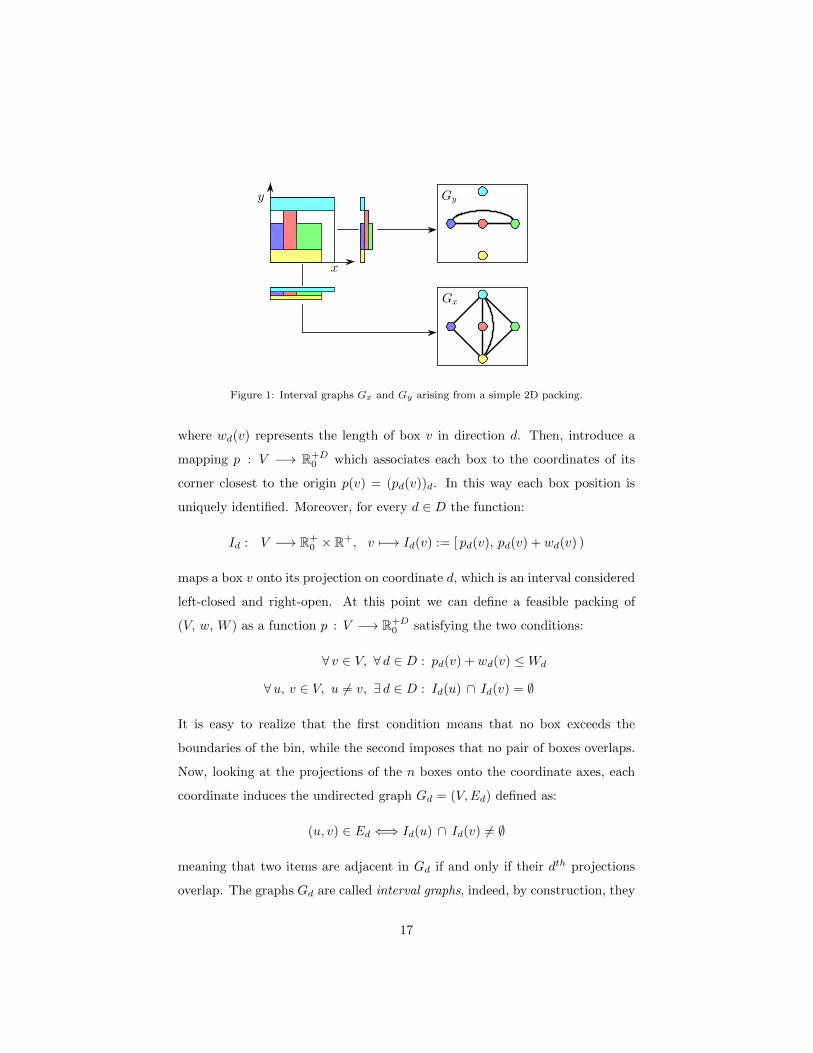
Intuitively, considering a set of boxes inside a bin and a specific coordinate axis,215

e.g. x, we can build a graph where:

• each node corresponds to a box

• an edge (u, v) is inserted in the graph if the projections of boxes u and v

on the x-axis overlap.

Figure 1 shows the construction of the interval graphs arising from a simple 2D220

packing.

The graph characterization of packings and its advantages are formally recalled

in the following. For simplicity, notation will be slightly different.

3.1. The graph characterization of packings

Consider a set of n D-dimensional parallelepipeds V , the bin size W = (Wd)d,

and define the size function w:

w : V −→ R+D, v 7−→ w(v) = (wd(v))d

16

Gx

Gy

x

y

Figure 1: Interval graphs Gx and Gy arising from a simple 2D packing.

where wd(v) represents the length of box v in direction d. Then, introduce a

mapping p : V −→ R+D0 which associates each box to the coordinates of its

corner closest to the origin p(v) = (pd(v))d. In this way each box position is

uniquely identified. Moreover, for every d ∈ D the function:

Id : V −→ R+0 × R+, v 7−→ Id(v) := [ pd(v), pd(v) + wd(v) )

maps a box v onto its projection on coordinate d, which is an interval considered

left-closed and right-open. At this point we can define a feasible packing of

(V, w, W ) as a function p : V −→ R+D0 satisfying the two conditions:

∀ v ∈ V, ∀ d ∈ D : pd(v) + wd(v) ≤Wd

∀u, v ∈ V, u 6= v, ∃ d ∈ D : Id(u) ∩ Id(v) = ∅

It is easy to realize that the first condition means that no box exceeds the

boundaries of the bin, while the second imposes that no pair of boxes overlaps.

Now, looking at the projections of the n boxes onto the coordinate axes, each

coordinate induces the undirected graph Gd = (V,Ed) defined as:

(u, v) ∈ Ed ⇐⇒ Id(u) ∩ Id(v) 6= ∅

meaning that two items are adjacent in Gd if and only if their dth projections

overlap. The graphs Gd are called interval graphs, indeed, by construction, they

17

are built from the intersection of intervals on the real line. We know from the

non-overlapping condition that an edge (u, v) cannot lie at the same time in Gd

for all d ∈ D. Furthermore, for all Gd a stable set S = v1, . . . , vk, i.e. a set of

pairwise nonadjacent nodes, fulfills:

k∑j=1

wd(vj) ≤Wd

meaning that boxes aligned on the axis d must have total length not greater than225

Wd. We call such a stable set d-feasible and sum up the previous observations

with a theorem.

Theorem 1. For any feasible packing, the induced graphs Gd = (V,Ed), d ∈ D,

have the following properties:

P1 : Gd is an interval graph

P2 : Each stable set of Gd is d-feasible

P3 : ∩dEd = ∅.

Fekete and Schepers showed that the reverse implication holds too and P1, P2,

P3 are sufficient to determine a feasible packing, but a few more concepts must

be recalled first.

An undirected graph G = (V, E) is said to be a comparability graph, or transi-

tively orientable graph, if there exists an orientation Φ of E which fulfills:

(a, b) ∈ Φ ∧ (b, c) ∈ Φ =⇒ (a, c) ∈ Φ

Such an orientation Φ is called a transitive orientation of E. Denoting Gd =

(V,Ed) the complement graph of Gd = (V,Ed), we know that if Gd arises from

a packing p, then Gd will be a comparability graph. Indeed, an edge in Gd

corresponds to two boxes with non-overlapping dth projection; hence we can

easily construct a transitive orientation Φd of Ed by defining:

(u, v) ∈ Φd ⇐⇒ (u, v) ∈ Ed ∧ pd(u) < pd(v)

18

i.e. projections of boxes u and v on axis d do not overlap, and the coordinate

of u is smaller than v. More generally, we deduce that the complement graph

of any interval graph is a comparability graph. The reverse implication does230

not hold as there exist some graphs which are not interval graphs and whose

complement is transitively orientable.

Finally, a family E = (Ed)d of edge sets for a vertex set V is called a packing

class for (V, w, W ) if it satisfies the three properties P1, P2, P3 and, given the

transitive orientations Φd of Gd for d ∈ D, we call the set Φ = (Φd)d a transitive235

orientation of the packing class E.

We can now state a second important result showing that any transitive ori-

entation Φ of E induces a packing pΦ and provides a method to find it by

construction.

Theorem 2. For a transitive orientation Φ of a packing class E, the function

pΦ : V −→ R+D0 defined as:

pΦd (v) :=

0 if @u ∈ V : (u, v) ∈ Φd

max pΦd (u) + wd(u) | (u, v) ∈ Φd otherwise

for v ∈ V and d ∈ D, represents a feasible packing.240

Theorem 2 constitutes the reverse implication of Theorem 1 and motivates the

graph characterization of packings. See [4] for a proof.

By construction, the packing pΦ introduced in Theorem 2 is lower gapless in

every direction d ∈ D, i.e. no item can be shifted to a position with lower

coordinates in some direction. Formally, a packing p for (V, w, W ) is said to

be lower gapless in direction d if for all v ∈ V , either v has a zero lower d

coordinate, pd(v) = 0, or it touches in direction d another box before it:

∃u ∈ V : pd(v) = pd(u) + wd(u) ∧ ∀ d′ 6= d : Id′(u) ∩ Id′(v) 6= ∅.

Analogously, we say a packing p for (V, w, W ) to be upper gapless in direction d

if for all v ∈ V , either v touches the upper wall of the bin, pd(v) +wd(v) = Wd,

19

or it touches in direction d another box after it:

∃u ∈ V : pd(v) + wd(v) = pd(u) ∧ ∀ d′ 6= d : Id′(u) ∩ Id′(v) 6= ∅

and we can define the upper gapless packing qΦ induced by a transitive orien-

tation Φ by:

qΦd (v) :=

Wd − wd(v) if @u ∈ V : (v, u) ∈ Φd

min qΦd (u)− wd(v) | (v, u) ∈ Φd otherwise.

To simplify notation, p and q will denote the two lower and upper gapless pack-

ings induced by a transitive orientation Φ, and pd, qd : V −→ R+0 their compo-

nents. The single components of p and q are defined mutually independent, thus

having Φ we can generate packings which are mixed lower and upper gapless

in the various directions, i.e. (pd1 , qd2), d1 ∈ D1, d2 ∈ D2, with D1, D2 a245

partition of D.

Introducing the gapless packings induced by a transitive orientation is important

when handling the load-balancing, as will be illustrated in the next section.

3.2. Basic balancing operations

Going back to the load-balancing problem, assume a bin-packing solution is

available and focus on a single bin. We want to rearrange items inside the bin

in order to make the barycenter of the bin as close as possible to the ideal point

Bopt. Given the packing p, it is possible to apply an overturning operation p:

p : V −→ R+D0 , v 7−→ p(v) := W − p(v)− w(v)

representing the symmetric packing of p w.r.t. the D hyperplanes which halve250

the bin at Wd/2. Note that the feasibility of the solution is obviously preserved

together with the gapless property (now upper instead of lower), and the op-

eration can be restricted to a single direction d ∈ D, leaving the remaining

coordinates unchanged. The same operation can be done with q, obtaining q.

Consider now the packing class E associated with the bin and its transitive255

orientation Φ. We can reallocate the boxes using four induced gapless packings,

20

p, q, p, q. Moreover, again, we can create a packing with mixed components pd,

qd, pd, qd as they act independently in the definition of p, q, p, q. Thus, a tran-

sitive orientation Φ induces 4D gapless packings, each of them with a different

barycenter.260

Let us focus on a single direction d and denote with Bpd , Bq

d, Bpd , Bq

d the dth

coordinate of the barycenter obtained with pd, qd, pd, qd respectively. We know

that Bpd ≤ B

qd and Bq

d ≤ Bpd .

Two cases are possible:

1. Boptd /∈ [Bp

d , Bqd ] ∪ [Bq

d, Bpd ]265

2. Boptd ∈ [Bp

d , Bqd ] ∪ [Bq

d, Bpd ]

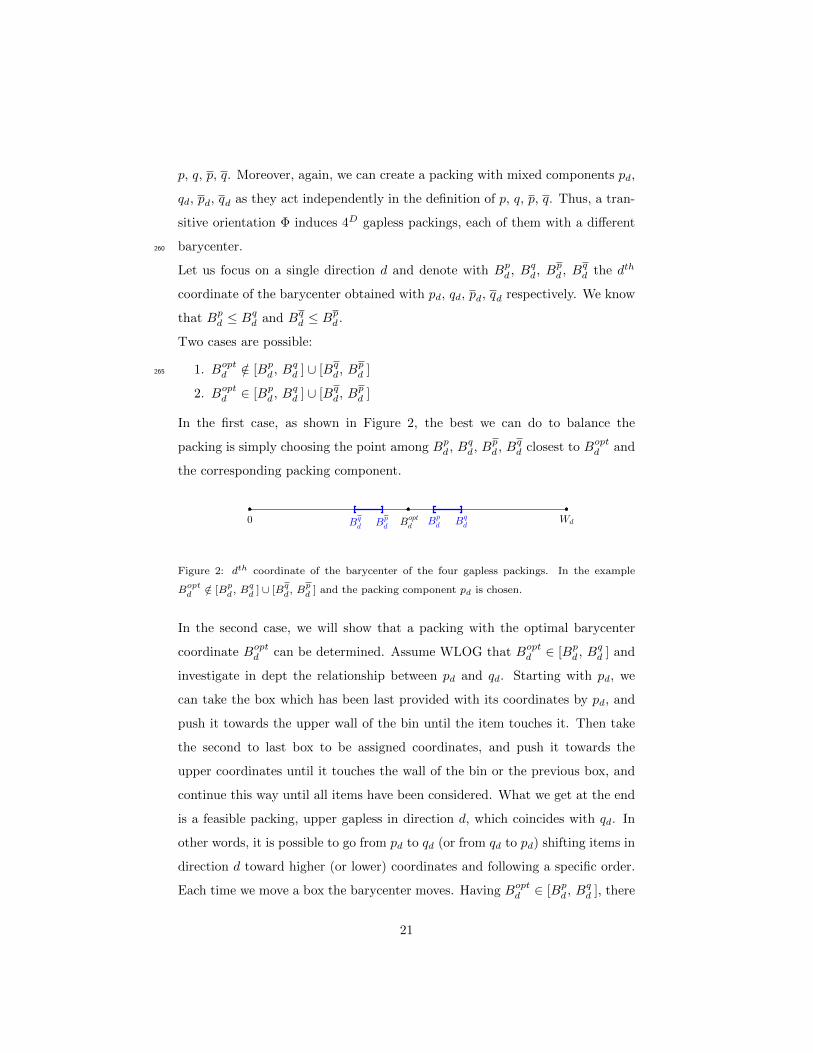
In the first case, as shown in Figure 2, the best we can do to balance the

packing is simply choosing the point among Bpd , Bq

d, Bpd , Bq

d closest to Boptd and

the corresponding packing component.

0 WdBpd B

qdB

pdB

qd

Boptd

Figure 2: dth coordinate of the barycenter of the four gapless packings. In the example

Boptd /∈ [Bp

d , Bqd ] ∪ [Bq

d, Bpd ] and the packing component pd is chosen.

In the second case, we will show that a packing with the optimal barycenter

coordinate Boptd can be determined. Assume WLOG that Bopt

d ∈ [Bpd , B

qd ] and

investigate in dept the relationship between pd and qd. Starting with pd, we

can take the box which has been last provided with its coordinates by pd, and

push it towards the upper wall of the bin until the item touches it. Then take

the second to last box to be assigned coordinates, and push it towards the

upper coordinates until it touches the wall of the bin or the previous box, and

continue this way until all items have been considered. What we get at the end

is a feasible packing, upper gapless in direction d, which coincides with qd. In

other words, it is possible to go from pd to qd (or from qd to pd) shifting items in

direction d toward higher (or lower) coordinates and following a specific order.

Each time we move a box the barycenter moves. Having Boptd ∈ [Bp

d , Bqd ], there

21

must be one item, say v, whose shift makes the barycenter crossing the optimal

dth coordinate Boptd , i.e. it moves from B1

d to B2d with B1

d ≤ Boptd ≤ B2

d. Then,

item v can be provided with a dth coordinate such that the barycenter is exactly

Boptd , simply using the proportion:

v 7−→ pd(v) +(B2

d −B1d

)−1(qd(v)− pd(v))

(Bopt

d −B1d

)Notice that if Bopt

d = 12 Wd, then for symmetry reasons the overturning is re-270

dundant.

To summarize, given a packing class with a transitive orientation, we can make

the barycenter closer to the ideal point by taking simple choices involving the

gapless packings induced by the orientation and performing basic operations as

moving iteratively boxes along one direction and overturning the packing. This275

is likely the best we can do right now with a specific transitive orientation, but

we will soon manage to find more transitive orientations of a packing class.

3.3. Local search at transitive orientation level

The goal of this section is to find a transitive orientation of a packing class

which leads, after performing the basic operations previously mentioned, to

a well-balanced packing. First, it is useful to determine how many transitive

orientations a comparability graph has and how to construct them. Terminology

and results of graph theory are needed and in the following only a few important

points will be mentioned. For an extensive background on the topic refer to

Golumbic [25].

It can be proven that the edges of an undirected graph G = (V,E) can be

uniquely partitioned into substructures M1, . . . ,Mk, called maximal multiplexes,

which act independently to transitive orientations. We say that E = M1 + · · ·+

Mk is the M -decomposition of the graph G.

To identify a maximal multiplex Mi, we first need to find a maximal simplex

Si, i.e. a complete subgraph with certain properties which can be built up

by local search from a single edge, and then make it grow using a particular

equivalent relation that forces adjacent edges to be part of the same structure.

22

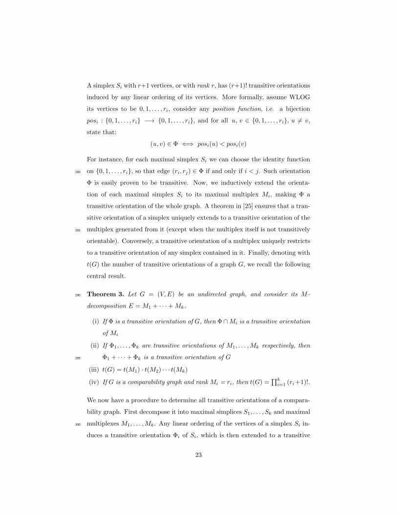
A simplex Si with r+1 vertices, or with rank r, has (r+1)! transitive orientations

induced by any linear ordering of its vertices. More formally, assume WLOG

its vertices to be 0, 1, . . . , ri, consider any position function, i.e. a bijection

posi : 0, 1, . . . , ri −→ 0, 1, . . . , ri, and for all u, v ∈ 0, 1, . . . , ri, u 6= v,

state that:

(u, v) ∈ Φ ⇐⇒ posi(u) < posi(v)

For instance, for each maximal simplex Si we can choose the identity function

on 0, 1, . . . , ri, so that edge (ri, rj) ∈ Φ if and only if i < j. Such orientation280

Φ is easily proven to be transitive. Now, we inductively extend the orienta-

tion of each maximal simplex Si to its maximal multiplex Mi, making Φ a

transitive orientation of the whole graph. A theorem in [25] ensures that a tran-

sitive orientation of a simplex uniquely extends to a transitive orientation of the

multiplex generated from it (except when the multiplex itself is not transitively285

orientable). Conversely, a transitive orientation of a multiplex uniquely restricts

to a transitive orientation of any simplex contained in it. Finally, denoting with

t(G) the number of transitive orientations of a graph G, we recall the following

central result.

Theorem 3. Let G = (V,E) be an undirected graph, and consider its M -290

decomposition E = M1 + · · ·+Mk.

(i) If Φ is a transitive orientation of G, then Φ ∩Mi is a transitive orientation

of Mi

(ii) If Φ1, . . . ,Φk are transitive orientations of M1, . . . ,Mk respectively, then

Φ1 + · · ·+ Φk is a transitive orientation of G295

(iii) t(G) = t(M1) · t(M2) · · · t(Mk)

(iv) If G is a comparability graph and rank Mi = ri, then t(G) =∏k

i=1 (ri+1)!.

We now have a procedure to determine all transitive orientations of a compara-

bility graph. First decompose it into maximal simplices S1, . . . , Sk and maximal

multiplexes M1, . . . ,Mk. Any linear ordering of the vertices of a simplex Si in-300

duces a transitive orientation Φi of Si, which is then extended to a transitive

23

orientation to Mi. The union of the Φi over all maximal multiplexes constitutes

a transitive orientation for the entire graph.

The next step is to move to the space of transitive orientations in order to find

a well-balanced packing. The analysis can be done for each coordinate indepen-305

dently of the others, so we focus on a single d ∈ D.

Given two transitive orientations Φ, Ψ of Gd, we evaluate them stating that Φ

is preferable to Ψ if fd(Φ) ≤ fd(Ψ), where fd(Φ) = |Boptd − Bd(Φ)| and Bd(Φ)

is the best barycenter we can obtain from Φ performing the basic balancing

operations (overturning, shifting items etc.) described in Section 3.2.310

The number of transitive orientations of Gd = (V,Ed) is a product of factorials,

t(Gd) =∏k

i=1(ri + 1)! where k is the number of maximal simplices and ri is

the rank of simplex i. If Ed itself is a clique, then t(Gd) assumes its maximum

possible value t(G) = |V |!. Such a number could potentially be huge. As a con-

sequence, instead of evaluating all transitive orientations, we will only explore315

a polynomial subset of orientations.

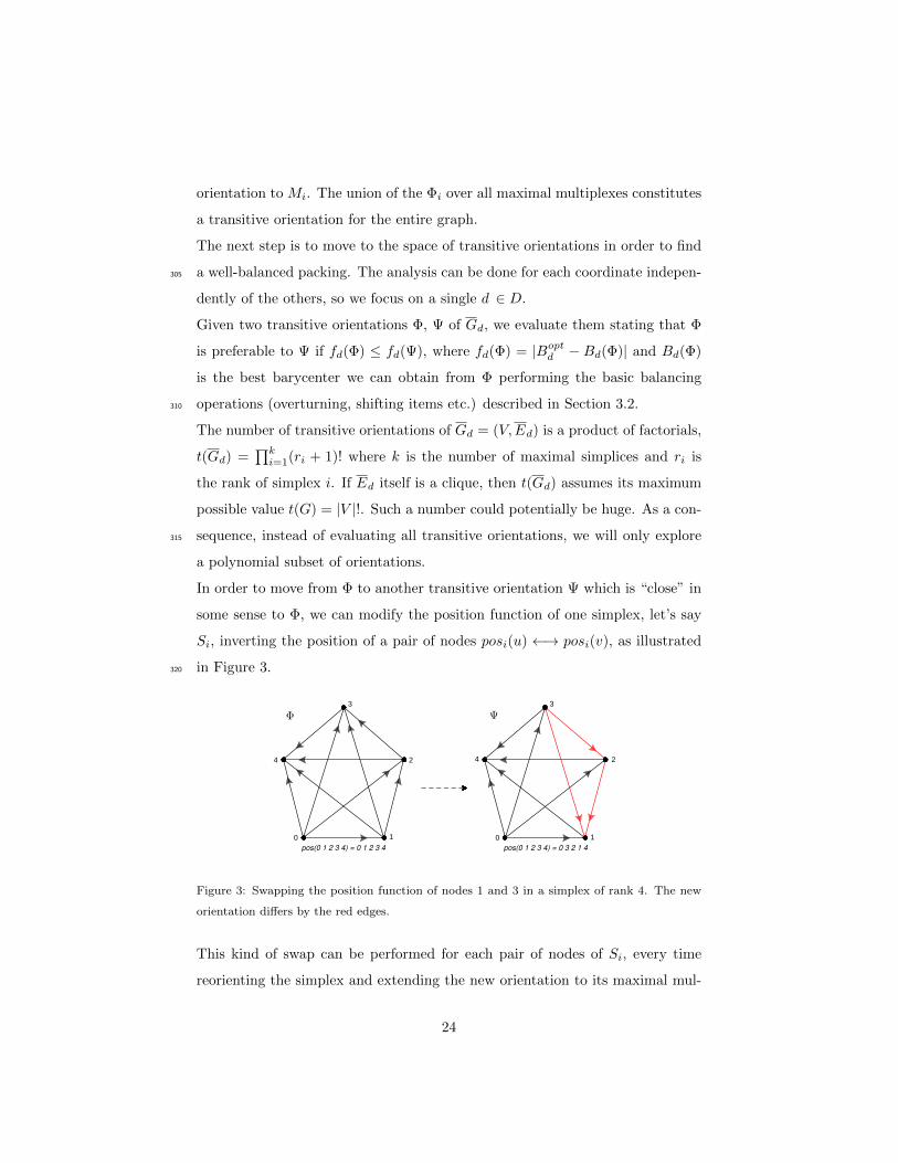
In order to move from Φ to another transitive orientation Ψ which is “close” in

some sense to Φ, we can modify the position function of one simplex, let’s say

Si, inverting the position of a pair of nodes posi(u) ←→ posi(v), as illustrated

in Figure 3.320

0 01 1

2 2

33

4 4

pos(0 1 2 3 4) = 0 1 2 3 4 pos(0 1 2 3 4) = 0 3 2 1 4

Φ Ψ

Figure 3: Swapping the position function of nodes 1 and 3 in a simplex of rank 4. The new

orientation differs by the red edges.

This kind of swap can be performed for each pair of nodes of Si, every time

reorienting the simplex and extending the new orientation to its maximal mul-

24

tiplex Mi to have a transitive orientation of the whole graph (in the meanwhile,

the other multiplexes with their orientation are left unchanged). If simplex Si

has rank ri, then the number of couples of nodes is ri(ri+1)/2, so we are consid-325

ering a quadratic subset of the total factorial number of transitive orientations

of simplex Si.

3.3.1. Balancing using transitive orientations: the algorithm

The algorithm is designed as a hill-climber heuristic and is here outlined. The

dimensions d ∈ D are considered separately one by one. First, decompose Gd

into maximal simplices and maximal multiplexes. Take the first simplex and

evaluate all the exchanges of vertice pairs w.r.t. the initial position function.

Save the best barycenter solution and its relative position function, then move to

the next simplex. The process is repeated until it has considered all simplices

without having found any improving solution, or when a maximum number

of iterations is reached. Finally, repeat the process for the other coordinates

d ∈ D.

The algorithm is classified as a local search method since we move from one

orientation Φ to a nearby one Ψ obtained by swapping the position of two

vertices in a simplex. The neighborhood of Φ is defined as the set of transitive

orientations generated from Φ by a swap in the position function of two nodes

in the same simplex. In particular, since we create a sequence of improving

solutions

fd(Φ0) > fd(Φ1) > · · · > fd(Φk)

the algorithm can be identified as a hill-climbing search. Moreover, we explore

the whole quadratic neighborhood of a simplex Si, pick up the best solution,330

and then go to Si+1. Thus, the algorithm is a best improvement search. It

could equally well have been defined as a first improvement search, indeed, in

several local search methods a first improvement strategy drastically reduces

the running time without degrading the solution quality. However, in our case

the best improvement search performed slightly better than first improvement.335

25

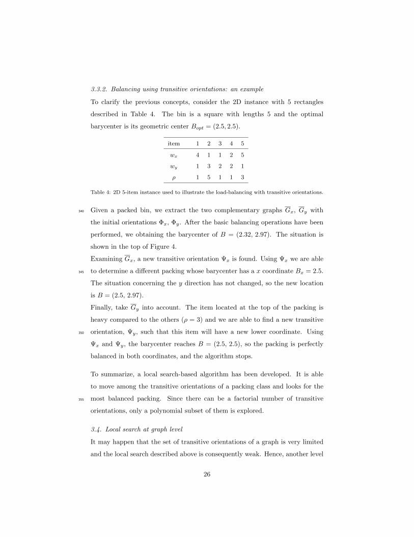
3.3.2. Balancing using transitive orientations: an example

To clarify the previous concepts, consider the 2D instance with 5 rectangles

described in Table 4. The bin is a square with lengths 5 and the optimal

barycenter is its geometric center Bopt = (2.5, 2.5).

item 1 2 3 4 5

wx 4 1 1 2 5

wy 1 3 2 2 1

ρ 1 5 1 1 3

Table 4: 2D 5-item instance used to illustrate the load-balancing with transitive orientations.

Given a packed bin, we extract the two complementary graphs Gx, Gy with340

the initial orientations Φx, Φy. After the basic balancing operations have been

performed, we obtaining the barycenter of B = (2.32, 2.97). The situation is

shown in the top of Figure 4.

Examining Gx, a new transitive orientation Ψx is found. Using Ψx we are able

to determine a different packing whose barycenter has a x coordinate Bx = 2.5.345

The situation concerning the y direction has not changed, so the new location

is B = (2.5, 2.97).

Finally, take Gy into account. The item located at the top of the packing is

heavy compared to the others (ρ = 3) and we are able to find a new transitive

orientation, Ψy, such that this item will have a new lower coordinate. Using350

Ψx and Ψy, the barycenter reaches B = (2.5, 2.5), so the packing is perfectly

balanced in both coordinates, and the algorithm stops.

To summarize, a local search-based algorithm has been developed. It is able

to move among the transitive orientations of a packing class and looks for the

most balanced packing. Since there can be a factorial number of transitive355

orientations, only a polynomial subset of them is explored.

3.4. Local search at graph level

It may happen that the set of transitive orientations of a graph is very limited

and the local search described above is consequently weak. Hence, another level

26

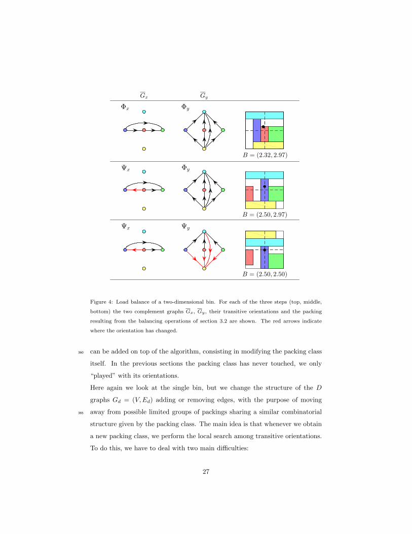
Φx Φy

Ψx Φy

Ψx Ψy

B = (2.50, 2.97)

B = (2.32, 2.97)

B = (2.50, 2.50)

Gx Gy

Figure 4: Load balance of a two-dimensional bin. For each of the three steps (top, middle,

bottom) the two complement graphs Gx, Gy , their transitive orientations and the packing

resulting from the balancing operations of section 3.2 are shown. The red arrows indicate

where the orientation has changed.

can be added on top of the algorithm, consisting in modifying the packing class360

itself. In the previous sections the packing class has never touched, we only

“played” with its orientations.

Here again we look at the single bin, but we change the structure of the D

graphs Gd = (V,Ed) adding or removing edges, with the purpose of moving

away from possible limited groups of packings sharing a similar combinatorial365

structure given by the packing class. The main idea is that whenever we obtain

a new packing class, we perform the local search among transitive orientations.

To do this, we have to deal with two main difficulties:

27

• How to modify a packing class in a clever way?

• How to verify that a new set of graphs still corresponds to a packing class?370

To modify the packing class we follow the approach of Crainic et al. [9]. The

authors proposed a neighborhood for a packing class, based on what they call

overlapping rules, and use it in the inner heuristic of a two-level tabu-search for

the 3D Bin-Packing Problem.

Basically, for each d and couple of items u 6= v in the bin, either (u, v) ∈ Ed if

u and v overlap in direction d, or (u, v) /∈ Ed if they do not. In the first case,

items can be made non-overlapping by removing edge (u, v) form Ed, whereas in

the second case they are made overlapping by adding (u, v) to Ed, but avoiding

the same edge being present in Ed for all d ∈ D.

In order to increase the probability for the new set of graphs to be a packing

class, some heuristic rules are used when adding or removing an edge. In par-

ticular, when (u, v) is added to Ed, a new edge set E′

d is built following the so

called add rule:

E′

d =Ed ∪ (u, v) ∪ (u, s) : pd(s) ≤ pd(v) ∧ pd(s) + wd(s) ≥ pd(v) + wd(v)

=Ed ∪ (u, v) ∪ (u, s) : Id(v) ⊆ Id(s)

meaning that if u and v overlap, then u and s must overlap too for each s such

that Id(v) ⊆ Id(s). Similarly, if (u, v) is removed from Ed, then we construct a

new edge set E′

d following the remove rule:

E′

d =Ed \ (u, v) ∪ (u, s) : pd(s) ≥ pd(v) ∧ pd(s) + wd(s) ≤ pd(v) + wd(v)

=Ed \ (u, v) ∪ (u, s) : Id(v) ⊇ Id(s)

where edges (u, s) are also removed from Ed if Id(v) ⊇ Id(s).

Once we have a new set of graphs Gd, we need to check if they correspond

to a packing class, i.e. whether conditions P1, P2 and P3 are fulfilled. From

graph theory we know that G is an interval graph if and only if G does not

contain any C4 chordless cycle, i.e. a chordless cycle with four nodes, and G is375

28

a comparability graph. Thus, from a computational point of view, the graphs

Gd = (V,Ed), d ∈ D represent a packing class if:

1. ∀ d, Gd does not contain any C4 chordless cycle

2. ∀ d, there exists a transitive orientation of Gd

3. ∀ d, every stable set of Gd is d-feasible380

4. ∩dEd = ∅.

Condition 1 is easy to check: for each (r, s), (t, u) ∈ Gd with r, s, t, u different

nodes, if the edges completing the C4 cycle (r, t), (s, u) exist, then one of the two

chords (r, u) or (s, t) must also exist. Condition 2 is checked using an algorithm

which verifies whether Gd is a comparability graph by building up one of its385

transitive orientations in O(δ|Ed|), where δ is the maximum degree of vertices

of Gd (see [25]). Condition 3 is equivalent to find the maximal weighted clique

of the complement Gd. In general, the Maximal Weighted Clique Problem is

NP-hard, but when restricted to comparability graphs it becomes tractable

and polynomially solvable. Lastly, Condition 4 is trivial to verify.390

The local search at graph level can be computationally expensive because every

edge (u, v) has 2D − 1 valid overlapping rules to test. Consequently, to keep a

low running time, when the number of vertices of the graph is high (> 18) this

phase is skipped and the search is limited to transitive orientations.

3.5. Local search at bin-packing level395

One last phase is added to the algorithm to remedy to possible bad initial bin-

packing solutions. It can be seen as a diversification phase which consists in

iteratively repacking and re-balancing proper n-tuples of weakly balanced bins.

First, bins are considered one after another and each of them is repacked from

scratch for a certain number of times using a constructive heuristic which in-400

cludes some randomness (e.g. in the initial sorting of its items). Doing this we

obtain different partial solutions to the bin-packing problem and, when a single

bin is still used, we balance it and keep the new packing in case of a balancing

improvement. This diversification phase has been introduced since the local

29

search in graphs alone may not be able to explore regions far from the initial405

packing class.

Secondly, similar operations are performed with n-tuples of bins, as described

below:

1. Scores are assigned to bins reflecting the current imbalance or the possi-

bility of balancing improvement. In particular, we defined two scores per410

bin: S1,i = f2i and S2,i = 1−Vi, where fi is the imbalance of bin i and Vi

is the percentage of volume filling in bin i.

2. k bins are randomly chosen with the operation usually called roulette

wheel selection, i.e. using probabilities proportional to the scores. In our

implementation, bin 1 out of k is chosen with score S1, and the remaining415

k − 1 bins with score S2.

3. The items in the k selected bins are merged and a randomized constructive

heuristic is used to recombine them.

4. If k bins are still used in the new solution, each of them is balanced.

When the imbalance sum over the k repacked bins decreases, the new420

partial packing is saved and the scores updated.

Before adopting such methodology, we need to choose the number k of bins to

repack.

We denote a k-neighborhood as the set of bin-packing solutions obtained by

repacking at least k bins (successfully, without increasing the number of used425

bins), i.e. solutions which differ in the packing of at most k bins with respect

to the initial packing. Since the size of k-neighborhoods increases exponentially

with k, we start considering couples (k = 2) as they are faster to explore. If no

balancing improvements are made in a predetermined number of iterations, the

search is extended to triples (k = 3) and so on until a maximum level of k (e.g.430

k = 8) is explored without any improving solution.

We also allow the search to go back to prior levels. In particular, after level

k > 2 is explored, we move back to level 2 if any improvement was made at level

k, otherwise we proceed to next level k + 1.

30

This approach is called variable-depth neighborhood search (VDNS) as the size435

of the k-neighborhood is not fixed but dynamically adjusts itself during the

search. See Ahuja et al. [26] or Pisinger and Ropke [27] for a detailed discussion

on VDNS.

Note that the L1-norm was necessary to build the MILP models in Chapter

2. For the heuristic algorithm any other measure of imbalance can be chosen440

instead, e.g. the Euclidean norm.

4. Computational results

The heuristic algorithm for the LB-MBP is now applied to several test cases. For

the experiments we will focus on the three-dimensional problem, but everything

discussed so far applies to any dimension.445

4.1. Finding the initial 3D bin-packing solution

We make use of a variant of the Extreme Point First Fit Decreasing heuristic

(EPFFD) [8], outlined here.

Boxes are initially sorted by non-increasing volume. Two consecutive boxes

may have a similar volume but a very different shape, e.g tall with small base

area vs. short and wide. If we swap their ordering and then apply an Extreme

Point-based algorithm, the final packing will be different and, if we are lucky, we

will save a bin. Thus, we start considering the “ideal” sorting by non-increasing

volume and, for each couple of consecutive boxes, we exchange their ordering

with a certain probability related to the ratio of their volume. The probability

pi of swapping box i and i+ 1 is defined by:

pi :=

5(

voli+1

voli− 0.9

)if voli+1

voli> 0.9

0 if voli+1

voli≤ 0.9

Therefore, for each box i, we compute pi, generate a random value r ∼ U(0, 1)

and swap i with i + 1 if r < pi. Labels are updated immediately after each

swap so that a box may shift more positions. After this operation we run the

31

EPFFD. Finally, the process is repeated for a fixed number of iterations and450

the best solution is saved.

We call this algorithm GRASP-Based EPFFD, or G-EPFFD, since the greedy

randomized initialization reminds us of the first part of the GRASP meta-

heuristic, although there is no succeeding search phase. Despite the simplicity

of the basic idea, G-EPFFD outperforms the Composite Extreme Point Best Fit455

Decreasing heuristic (C-EPBFD) [8] and likely performs similarly to many of

the state-of-the-art meta-heuristics for the 3D bin-packing, while having run-

ning time under one second even for large instances. G-EPFFD will be used as

starting solution for the load balancing phase.

4.2. Repacking during VDNS460

Concerning the recombination of k bins during the VDNS, the EPFFD is used

with the minor modification consisting in loading the ordered items (by non-

increasing volume) one after another into the first bin in which they fit, where

the k available bins are randomly permuted after each item insertion. In this

way the probability of repacking within k bins is kept high; at the same time465

items are better redistributed among the bins avoiding situations where the first

bin contains all the very small items and is hence difficult to balance.

In principle, one is free to use any other packing heuristic for the recombination

phase. However, it is important to include some element of stochasticity and to

maintain the running time very low since the repacking is potentially computed470

thousands of times during the VDNS.

4.3. Load Balancing

The multi-level local search algorithm is used to balance the initial bin-packing

solution obtained from G-EPFFD on a variety of test cases summarized in Tables

5 and 6.475

The desired barycenter location is the center of the bin Bopt = 0.5 (Wx,Wy,Wz)

in Table 5 and the center of the base of the bin Bopt = 0.5 (Wx,Wy, 0) in Table

6. Classes 1-8 are standard instances for the 3D Bin-Packing Problem from the

32

literature [3] tested with 100 and 200 items. Columns 3 and 4 contain the lower

bound on the number of bins and the G-EPFFD solution respectively. Each480

class is then tested with three different density distributions of items:

1. same density for all items, ρi = 1

2. small density variance, ρi ∼ U(1, 2)

3. high density variance, ρi ∼ U(1, 6)

For every test case we measured how the balancing component of the objective485

function (14) decreases when the different search levels are used, keeping the

weights kx = ky = kz = 1. The first phase (Ph 1) represents the imbalance

value immediately after G-EPFFD is applied, the second phase (Ph 2) gives

the value after each bin is balanced, the last phase (Ph 3) indicates the final

imbalance value after VDNS is performed.490

To allow a comparison between different test cases, entries of Tables 5 and 6 are

normalized so that they contain the mean imbalance value per individual bin,

and refer to bins of edge length 100. Moreover, all entries are averages over 25

instances.

The algorithm has been implemented in C and run on an Intel Core i5 with495

8GB RAM. The average running time varies from a few seconds (Table 5, class

1-4) to a few minutes (Table 6, class 5).

When the optimal barycenter is the center of the bin (Table 5), a lower bound

for the balancing component is trivially zero, corresponding to zero imbalance500

in every direction for all bins and hence leading to an easy interpretation of the

results.

After each bin is individually balanced (Ph 2), the objective value is greatly

improved and on average more than 90% of the total initial imbalance is removed

from the packing. The last balancing phase (Ph 3) has also a considerable effect,505

bringing the objective value very close to zero in most of the cases and showing

once again the limits of the sequential packing and balancing approach (Ph 1 +

Ph 2) compared to a unified approach where the balancing potential of having

33

Foo

Bopt=center of the bin ρi = 1 ρi ∼ U(1, 2) ρi ∼ U(1, 6)

class size LB bins Ph 1 Ph 2 Ph 3 Ph 1 Ph 2 Ph 3 Ph 1 Ph 2 Ph 3

1 100 24.12 25.64 16.48 0.91 0.011 17.03 0.68 0.054 19.22 2.26 0.201

2 100 24.64 26.12 16.19 0.85 0.011 16.69 0.68 0.042 19.01 2.28 0.198

3 100 24.48 26.08 16.34 0.87 0.006 16.78 0.66 0.030 19.16 2.21 0.245

4 100 57.44 60.60 31.74 0.58 0.011 30.64 0.29 0.030 30.91 0.93 0.090

5 100 13.60 14.60 15.83 0.92 0.003 15.87 0.71 0.068 17.65 2.70 0.425

6 100 18.20 20.08 9.83 1.45 0.190 10.30 1.70 0.396 13.49 4.54 1.210

7 100 11.12 12.36 16.89 1.19 0.012 16.53 0.79 0.050 18.37 3.11 0.559

8 100 15.52 17.08 15.66 0.78 0.008 15.34 0.64 0.056 17.35 2.63 0.501

1 200 48.84 51.16 15.05 0.79 0.007 15.74 0.82 0.032 18.36 2.57 0.208

2 200 48.48 50.80 14.81 0.77 0.006 15.57 0.85 0.044 18.24 2.58 0.217

3 200 49.24 51.24 14.91 0.77 0.005 15.68 0.83 0.036 18.29 2.65 0.262

4 200 117.8 122.2 31.91 0.53 0.004 30.66 0.29 0.012 30.91 0.96 0.034

5 200 25.60 27.36 12.47 0.75 0.011 13.06 0.89 0.147 14.90 3.23 0.801

6 200 35.84 38.24 6.74 1.30 0.241 8.17 2.19 0.523 12.09 5.44 1.505

7 200 20.36 22.40 12.72 1.26 0.057 12.95 1.15 0.329 14.89 3.99 1.567

8 200 29.40 32.04 12.75 0.70 0.016 12.79 0.98 0.183 14.66 3.33 0.921

Table 5: Multi-level local search heuristic for LB-MBP (3D case) when optimal barycenter is

the center of the container

a large number of packing solutions with the same number of bins is exploited.

We notice that it is easier to arrange equally dense items in the bin space so that510

the barycenter falls close to the center of the bin. Such a task is more difficult

when some very dense item is present and the balancing is consequently slightly

worse.

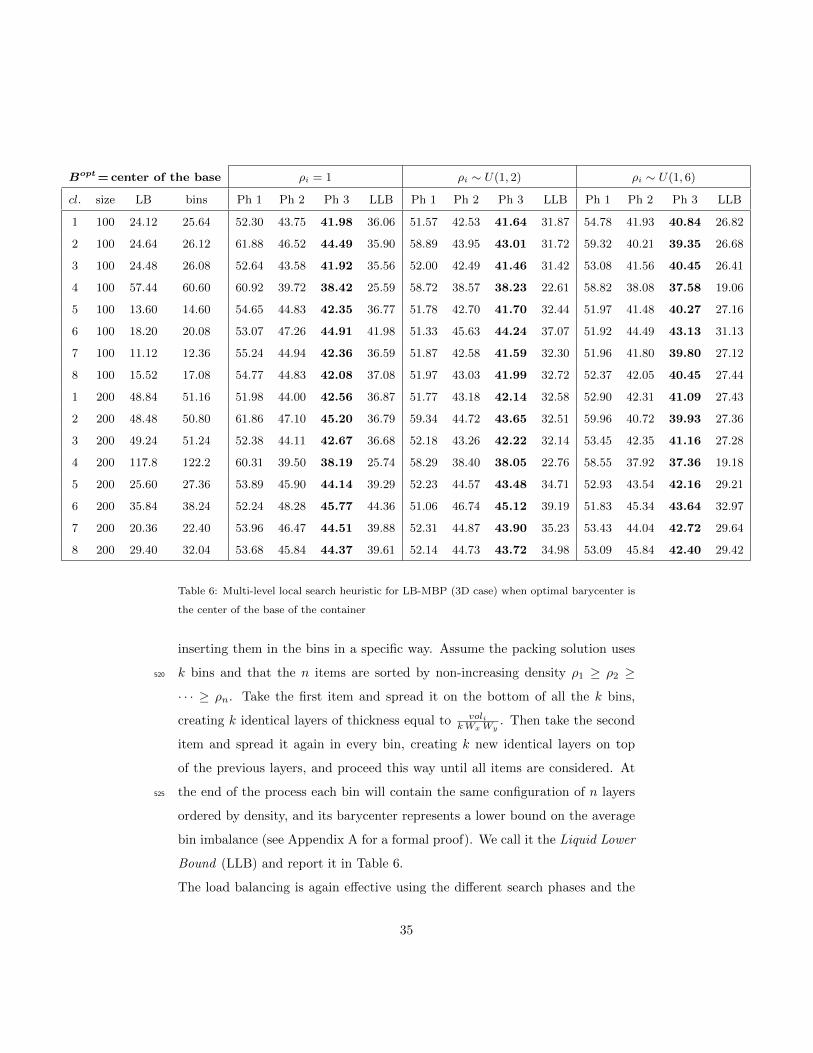
When the optimal barycenter is the center of the base of the container (Table

6), zero is still an obvious lower bound but not tight enough to be somehow515

useful. The bin imbalance may be zero on the x and y directions, but it will

always be strictly positive on z.

It is possible to construct a new lower bound by “liquifying” the items and

34

Bopt=center of the base ρi = 1 ρi ∼ U(1, 2) ρi ∼ U(1, 6)

cl. size LB bins Ph 1 Ph 2 Ph 3 LLB Ph 1 Ph 2 Ph 3 LLB Ph 1 Ph 2 Ph 3 LLB

1 100 24.12 25.64 52.30 43.75 41.98 36.06 51.57 42.53 41.64 31.87 54.78 41.93 40.84 26.82

2 100 24.64 26.12 61.88 46.52 44.49 35.90 58.89 43.95 43.01 31.72 59.32 40.21 39.35 26.68

3 100 24.48 26.08 52.64 43.58 41.92 35.56 52.00 42.49 41.46 31.42 53.08 41.56 40.45 26.41

4 100 57.44 60.60 60.92 39.72 38.42 25.59 58.72 38.57 38.23 22.61 58.82 38.08 37.58 19.06

5 100 13.60 14.60 54.65 44.83 42.35 36.77 51.78 42.70 41.70 32.44 51.97 41.48 40.27 27.16

6 100 18.20 20.08 53.07 47.26 44.91 41.98 51.33 45.63 44.24 37.07 51.92 44.49 43.13 31.13

7 100 11.12 12.36 55.24 44.94 42.36 36.59 51.87 42.58 41.59 32.30 51.96 41.80 39.80 27.12

8 100 15.52 17.08 54.77 44.83 42.08 37.08 51.97 43.03 41.99 32.72 52.37 42.05 40.45 27.44

1 200 48.84 51.16 51.98 44.00 42.56 36.87 51.77 43.18 42.14 32.58 52.90 42.31 41.09 27.43

2 200 48.48 50.80 61.86 47.10 45.20 36.79 59.34 44.72 43.65 32.51 59.96 40.72 39.93 27.36

3 200 49.24 51.24 52.38 44.11 42.67 36.68 52.18 43.26 42.22 32.14 53.45 42.35 41.16 27.28

4 200 117.8 122.2 60.31 39.50 38.19 25.74 58.29 38.40 38.05 22.76 58.55 37.92 37.36 19.18

5 200 25.60 27.36 53.89 45.90 44.14 39.29 52.23 44.57 43.48 34.71 52.93 43.54 42.16 29.21

6 200 35.84 38.24 52.24 48.28 45.77 44.36 51.06 46.74 45.12 39.19 51.83 45.34 43.64 32.97

7 200 20.36 22.40 53.96 46.47 44.51 39.88 52.31 44.87 43.90 35.23 53.43 44.04 42.72 29.64

8 200 29.40 32.04 53.68 45.84 44.37 39.61 52.14 44.73 43.72 34.98 53.09 45.84 42.40 29.42

Table 6: Multi-level local search heuristic for LB-MBP (3D case) when optimal barycenter is

the center of the base of the container

inserting them in the bins in a specific way. Assume the packing solution uses

k bins and that the n items are sorted by non-increasing density ρ1 ≥ ρ2 ≥520

· · · ≥ ρn. Take the first item and spread it on the bottom of all the k bins,

creating k identical layers of thickness equal to volikWx Wy

. Then take the second

item and spread it again in every bin, creating k new identical layers on top

of the previous layers, and proceed this way until all items are considered. At

the end of the process each bin will contain the same configuration of n layers525

ordered by density, and its barycenter represents a lower bound on the average

bin imbalance (see Appendix A for a formal proof). We call it the Liquid Lower

Bound (LLB) and report it in Table 6.

The load balancing is again effective using the different search phases and the

35

imbalance decreases on average by 20% after Ph 2 and by additional 3-4% after530

Ph 3. The gap from LLB remains quite high around 20-25%; however, given

the small gaps achieved in Table 5, we tend to believe that in Table 6 we are

also not far from the optimal balancing.

LLB is clearly not very tight for a general instance since we are introducing two

different kinds of relaxations: the 3D shape of items is liquefied and items are535

splittable into more bins. We suspect it is possible to construct a tighter lower

bound by exploiting the unsplittable and 3D shape of items with combinatorial

logic. This task, together with providing bounds for the general case when the

desired barycenter is neither the center of the bin nor the center of its base, is

left to further research.540

Finally, we notice that the balancing value is now slightly better when densities

vary a lot from each other. Indeed it is possible to locate heavy items at the

bottom of the bin, moving down the barycenter.

5. Conclusions

In this paper, we presented the load-balanced multi-dimensional bin-packing545

problem, aimed at developing an integrated model of the multi-dimensional bin

packing with the load balancing of bins. The problem has only been considered

in the literature in simplified versions (e.g. balancing a single bin or introduc-

ing a feasible region for the barycenter) and is here treated in its natural full

formulation.550

We developed a mathematical programming model able to optimally solve smaller

instances of the problem, and defined a multi-level local search heuristic able

to handle large instances. Main ingredients of the heuristic are the graph rep-

resentation of packings, the analysis of the transitive orientations of a graph,

the extreme point-based algorithms for the packing phases and the dynamical555

recombination of n-tuples of weakly balanced bins.

Computational experiments were promising, showing that an effective load bal-

ancing can be obtained. Moreover, despite the intrinsic complexity of the algo-

36

rithm (many stages nested into each other), the running time of the heuristic

is usually very low and rarely exceeds 3-5 minutes even for difficult or large560

instances with 200 items, making the algorithm applicable in a set of real-life

logistic problems.

Acknowledgments

The authors would like to thank Prof. Marco Trubian and Dr. Fabio Colombo,

University of Milan, for the useful suggestions provided to this work.565

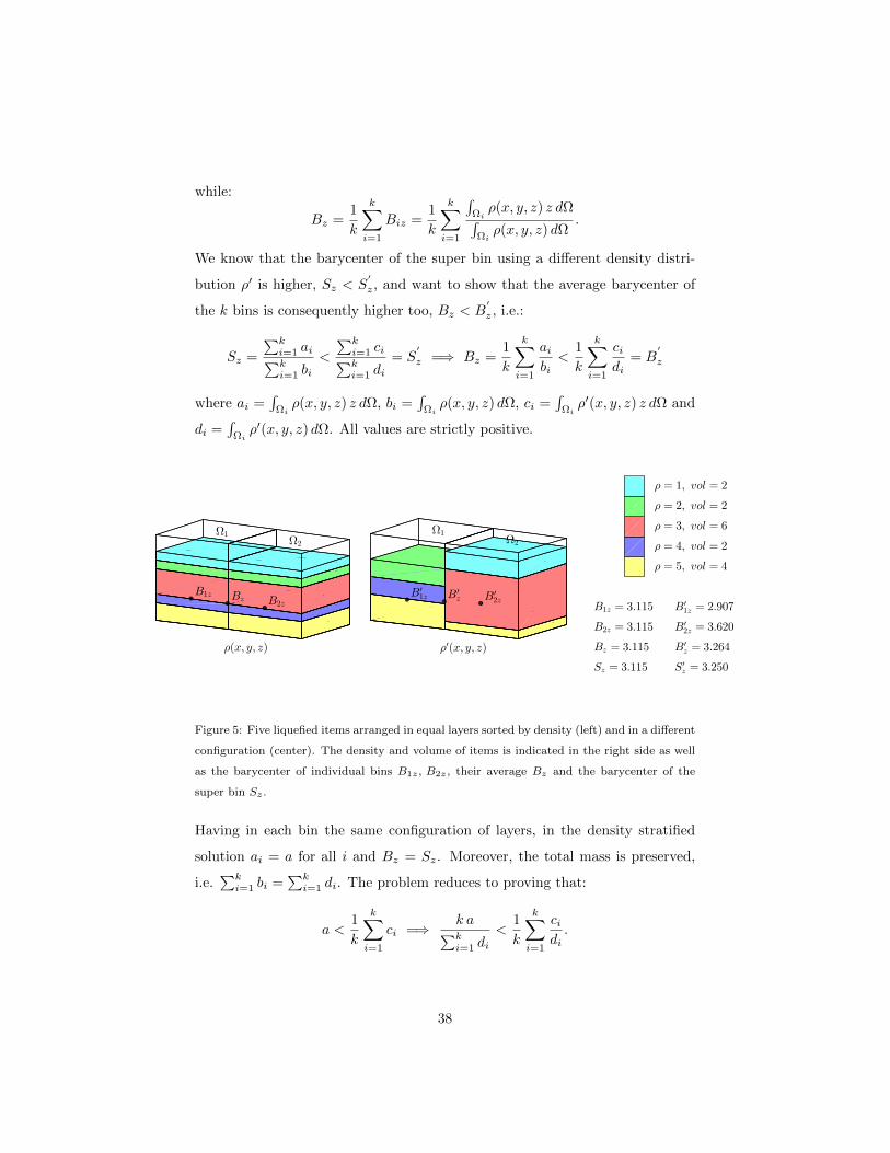
Appendix A. Liquid lower bound

In order to prove that LLB represents a lower bound, we show that the average

barycenter of k containers filled with any different arrangement of liquefied items

(not necessarily by layers) would be higher.

Let us call Ωi, i = 1, . . . , k the 3D volume occupied by container i, and dispose

the liquefied items into the containers in a different way. Assume containers are

stick together and remove the separating walls, obtaining one super bin which

occupies a 3D volume Ω = ∪iΩi. It is known from fluid dynamics that the state

of lowest potential energy in this super bin corresponds to the horizontal density

stratification where lightest fluids are on the top, as in LLB (see for instance

[28]). A lower potential energy of the system implies a lower barycenter, being

the potential energy U =∫

Ωρ(x, y, z) g z dΩ proportional to the zth coordinate

of the barycenter Sz = 1M

∫Ωρ(x, y, z) z dΩ, with M =

∫Ωρ(x, y, z) dΩ total

mass.

Notice that the zth coordinate of the barycenter of the super bin, Sz, does not

necessarily coincide with the average zth coordinate of the barycenter of the k

bins, Bz, as shown in the example of Figure 5. Let us analyze the relationship

between these two values.

Sz =1

M

∫Ω

ρ(x, y, z) z dΩ =

∫Ωρ(x, y, z) z dΩ∫

Ωρ(x, y, z) dΩ

=

∑ki=1

∫Ωiρ(x, y, z) z dΩ∑k

i=1

∫Ωiρ(x, y, z) dΩ

37

while:

Bz =1

k

k∑i=1

Biz =1

k

k∑i=1

∫Ωiρ(x, y, z) z dΩ∫

Ωiρ(x, y, z) dΩ

.

We know that the barycenter of the super bin using a different density distri-

bution ρ′ is higher, Sz < S′

z, and want to show that the average barycenter of

the k bins is consequently higher too, Bz < B′

z, i.e.:

Sz =

∑ki=1 ai∑ki=1 bi

<

∑ki=1 ci∑ki=1 di

= S′

z =⇒ Bz =1

k

k∑i=1

aibi<

1

k

k∑i=1

cidi

= B′

z

where ai =∫

Ωiρ(x, y, z) z dΩ, bi =

∫Ωiρ(x, y, z) dΩ, ci =

∫Ωiρ′(x, y, z) z dΩ and

di =∫

Ωiρ′(x, y, z) dΩ. All values are strictly positive.

Ω2

B2z

ρ(x, y, z)

Bz

Ω1

B1z

Ω2

B′

2z

ρ′(x, y, z)

B′

z

Ω1

B′

1z

B1z = 3.115

B2z = 3.115

Bz = 3.115

Sz = 3.115

B′

1z = 2.907

B′

2z = 3.620

B′

z = 3.264

S′

z = 3.250

ρ = 5, vol = 4

ρ = 4, vol = 2

ρ = 3, vol = 6

ρ = 2, vol = 2

ρ = 1, vol = 2

Figure 5: Five liquefied items arranged in equal layers sorted by density (left) and in a different

configuration (center). The density and volume of items is indicated in the right side as well

as the barycenter of individual bins B1z , B2z , their average Bz and the barycenter of the

super bin Sz .

Having in each bin the same configuration of layers, in the density stratified

solution ai = a for all i and Bz = Sz. Moreover, the total mass is preserved,

i.e.∑k

i=1 bi =∑k

i=1 di. The problem reduces to proving that:

a <1

k

k∑i=1

ci =⇒ k a∑ki=1 di

<1

k

k∑i=1

cidi.

38

Set ci = a+ ti, then∑k

i=1 ti > 0 and:

1

k

k∑i=1

cidi

=1

k

k∑i=1

a+ tidi

=1

k

k∑i=1

a

di+

1

k

k∑i=1

tidi>

1

k

k∑i=1

a

di=a

k

k∑i=1

1

di.

Finally, the relation

1

k

k∑i=1

1

di≥ k∑k

i=1 di

holds as direct consequence of the inequality of arithmetic and geometric means.

This inequality states that given a list of k nonnegative real numbers r1, r2, . . . , rk,

the arithmetic mean of the list is always greater or equal than the geometric

mean, i.e.:

1

k

k∑i=1

ri ≥

(k∏

i=1

ri

)1/k

.

Substituting ri = 1/di and applying the inequality of arithmetic and geometric

means twice, we obtain:

1

k

k∑i=1

1

di≥

(k∏

i=1

1

di

)1/k

=1(∏k

i=1 di

)1/k≥ 1

1k

∑ki=1 di

=k∑k

i=1 di.

In conclusion, for any start configuration, it is possible to move to the LLB

solution by decreasing the average barycenter of the k bins. The LLB value570

is therefore the lowest possible and a valid lower bound for our optimization

problem.

References

[1] M. Mongeau, C. Bes, Optimization of aircraft container loading, IEEE

Transactions on Aerospace and Electronic Systems 39 (1) (2003) 140–150.575

[2] S. Martello, D. Vigo, Exact solution of the two-dimensional finite bin pack-

ing problem, Management Science 44 (3) (1998) 388–399.

[3] S. Martello, D. Pisinger, D. Vigo, The three-dimensional bin packing prob-

lem, Operations Research 48 (2) (2000) 256–267.

39

[4] S. P. Fekete, J. Schepers, A combinatorial characterization of higher-580

dimensional orthogonal packing, Mathematics of Operations Research

29 (2) (2004) 353–368.

[5] S. P. Fekete, J. Schepers, J. C. van der Veen, An exact algorithm for higher-

dimensional orthogonal packing, Operations Research 55 (3) (2007) 569–

587.585

[6] A. Lodi, S. Martello, D. Vigo, Tspack: A unified tabu search code for

multi-dimensional bin packing problems, Annals of Operations Research

131 (2004) 203–213.

[7] O. Faroe, D. Pisinger, M. Zachariasen, Guided local search for the three-

dimensional bin-packing problem, INFORMS Journal on Computing 15 (3)590

(2003) 267–283.

[8] T. G. Crainic, G. Perboli, R. Tadei, Extreme point-based heuristics for

three-dimensional bin packing, INFORMS Journal on Computing 20 (3)

(2008) 368–384.

[9] T. G. Crainic, G. Perboli, R. Tadei, Ts2pack: A two-level tabu search for595

the three-dimensional bin packing problem, European Journal of Opera-

tional Research 195 (3) (2009) 744–760.

[10] T. G. Crainic, G. Perboli, R. Tadei, An efficient metaheuristic for multi-

dimensional multi-container packing, IEEE Conference on Automation Sci-

ence and Engineering (2011) 563–568.600

[11] J. Egeblad, D. Pisinger, Heuristic approaches for the two- and three-

dimensional knapsack packing problem, Computers & Operations Research

36 (4) (2009) 1026–1049.

[12] A. Lodi, S. Martello, D. Vigo, Heuristic algorithms for the three-

dimensional bin packing problem, European Journal of Operational Re-605

search 141 (2) (2002) 410–420.

40

[13] D. Pisinger, M. Sigurd, Using decomposition techniques and constraint pro-

gramming for solving the two-dimensional bin-packing problem, INFORMS

Journal on Computing 19 (1) (2007) 36–51.

[14] A. Davies, E. E. Bischoff, Weight distribution considerations in container610

loading, European Journal of Operational Research 114 (3) (1999) 509–527.

[15] L. Junqueira, R. Morabito, D. S. Yamashita, Three-dimensional container

loading models with cargo stability and load bearing constraints, Comput-

ers & Operations Research 39 (1) (2012) 74–85.

[16] C. Paquay, M. Schyns, S. Limbourg, A mixed integer programming for-615

mulation for the three-dimensional bin packing problem deriving from an

air cargo application, International Transactions in Operational Research

23 (1-2) (2016) 187–213.

[17] B. L. Kaluzny, R. H. A. D. Shaw, Optimal aircraft load balancing, Inter-

national Transactions in Operational Research 16 (6) (2009) 767–787.620

[18] M. M. Baldi, G. Perboli, R. Tadei, The three-dimensional knapsack prob-

lem with balancing constraints, Applied Mathematics and Computation

218 (19) (2012) 9802–9818.

[19] T. A. de Queiroz, F. K. Miyazawa, Two-dimensional strip packing problem

with load balancing, load bearing and multi-drop constraints, International625

Journal of Production Economics 145 (2) (2013) 511–530.

[20] A. Fernandez, C. Gil, R. Banos, M. G. Montoya, A parallel multi-objective

algorithm for two-dimensional bin packing with rotations and load balanc-

ing, Expert Systems with Applications 40 (13) (2013) 5169–5180.

[21] D. Liu, K. Tan, S. Huang, C. Goh, W. Ho, On solving multiobjective bin630

packing problems using evolutionary particle swarm optimization, Euro-

pean Journal of Operational Research 190 (2) (2008) 357–382.

41

[22] A. Imai, K. Sasaki, E. Nishimura, S. Papadimitriou, Multi-objective si-

multaneous stowage and load planning for a container ship with container

rehandle in yard stacks, European Journal of Operational Research 171 (2)635

(2006) 373–389.

[23] M. R. Garey, R. L. Graham, D. S. Johnson, A. C.-C. Yao, Resource con-

strained scheduling as generalized bin packing, Journal of Combinatorial

Theory, Series A 21 (3) (1976) 257–298.

[24] C. E. Miller, A. W. Tucker, R. A. Zemlin, Integer programming formulation640

of traveling salesman problems, Journal of the ACM (JACM) 7 (4) (1960)

326–329.

[25] M. C. Golumbic, Algorithmic graph theory and perfect graphs, 2nd Edition,

Elsevier, 2004.

[26] R. K. Ahuja, E. Ozlem, J. B. Orlin, A. P. Punnen, A survey of very645

large-scale neighborhood search techniques, Discrete Applied Mathemat-

ics 123 (1-3) (2002) 75–102.

[27] D. Pisinger, S. Ropke, Large neighborhood search, in: Handbook of Meta-

heuristics, Springer, 2010, Ch. 13, pp. 399–419.

[28] B. Cushman-Roisin, J.-M. Beckers, Introduction to geophysical fluid dy-650

namics: physical and numerical aspects, 2nd Edition, Elsevier, 2011.

42