arX

iv:a

stro

-ph/

0512

104v

2 2

8 Fe

b 20

06

Cluster Masses from CMB and Galaxy Weak Lensing

Antony Lewis1, ∗ and Lindsay King1

1Institute of Astronomy, Madingley Road, Cambridge, CB3 0HA, UK.

Gravitational lensing can be used to directly constrain the projected density profile of galaxy clus-ters. We discuss possible future constraints using lensing of the CMB temperature and polarization,and compare to results from using galaxy weak lensing. We model the moving lens and kinetic SZsignals that confuse the temperature CMB lensing when cluster velocities and angular momenta areunknown, and show how they degrade parameter constraints. The CMB polarization cluster lensingsignal is ∼ 1µK for massive clusters and challenging to detect; however it should be significantlycleaner than the temperature signal and may provide the most robust constraints at low noise levels.Galaxy lensing is likely to be much better for constraining cluster masses at low redshift, but forclusters at redshift z & 1 future CMB lensing observations may be able to do better.

I. INTRODUCTION

The distribution of clusters of galaxies as a function of mass and redshift depends on the cosmological model,and can be modelled increasingly accurately [1, 2, 3, 4]. Observations of clusters can therefore be used to learnabout cosmology, as well as to test models for cluster formation and evolution. Observations of the thermal Sunyaev-Zel’dovich (SZ) effect [1, 3, 5] are a powerful probe of the cluster gas, but do not measure the mass directly. To relatethe gas properties to the total mass involves modelling potentially complicated baryonic gas physics. By contrastgravitational lensing probes the projected total mass, not just the gas, and therefore can provide direct informationabout cluster masses. In this paper we analyse the potential for reconstruction of parameterized cluster profilesfrom future observations of cluster lensing of the CMB and weak lensing of distant galaxies. For the first time weinclude constraints from CMB polarization, and also include a model of the moving lens effect that confuses the CMBtemperature signal when the clusters have unknown velocities. The CMB polarization signal is much cleaner thanthe temperature at low noise levels, and may prove to be a good way to constrain cluster masses at high redshift.We perform an essentially optimal statistical analysis in the approximation that the unlensed fields can be treated asGaussian.Current CMB observations are not of high enough resolution or sensitivity to measure the cluster lensing signal.

However, future missions aimed at detecting small levels of primordial gravitational waves via their distinct B-modepolarization signal will require both high sensitivity and resolution. This is because lensing by large scale structurecan convert scalar E-modes into B-modes, and hence this lensing signal has to be subtracted to extract a smallprimordial B-mode signal from gravitational waves. The lensing reconstruction requires high resolution observationsin order to have enough information to solve for both the primordial B-modes and the unknown large scale structuredistribution [6]. It is therefore of interest to see what other useful information can be gained from such future highresolution observations. The resolution required for B-mode cleaning is probably rather less than needed for goodcluster mass constraints from CMB lensing, however it is clearly of interest to see what can be gained from observationswith slightly higher arcminute-level resolution. Cluster lensing of CMB temperature and polarization that we considerhere is one potentially useful possibility.Cluster lensing also generates a shear field that is observable by looking at the shapes of galaxies lying behind

the cluster. This method of cluster mass constraint is promising and possible with current observations, though atsome level has to be limited by the finite number of source galaxies available behind the lens. The seminal paperof Kaiser & Squires [7] describes how to do a non-parametric mass reconstruction; this technique and its variantshave been applied to numerous clusters (e.g. Refs. [8, 9]). Here we focus on parameterized cluster models, whichenable statistical comparisons to be made between clusters and as a function of observational strategy. The likelihoodtechniques are based on those developed in Refs. [10, 11]. We shall investigate how galaxy lensing compares to CMBlensing as a function of noise level, cluster redshift and galaxy number count. We use natural units where the speedof light is unity.

∗URL: http://cosmologist.info

2

−3 −2 −1 0 1 2 3

−3

−2

−1

0

1

2

3

−100

−80

−60

−40

−20

0

20

40

60

80

100

−3 −2 −1 0 1 2 3

−3

−2

−1

0

1

2

3

−100

−80

−60

−40

−20

0

20

40

60

80

100

−3 −2 −1 0 1 2 3

−3

−2

−1

0

1

2

3

µ K

−10

−8

−6

−4

−2

0

2

4

6

8

10

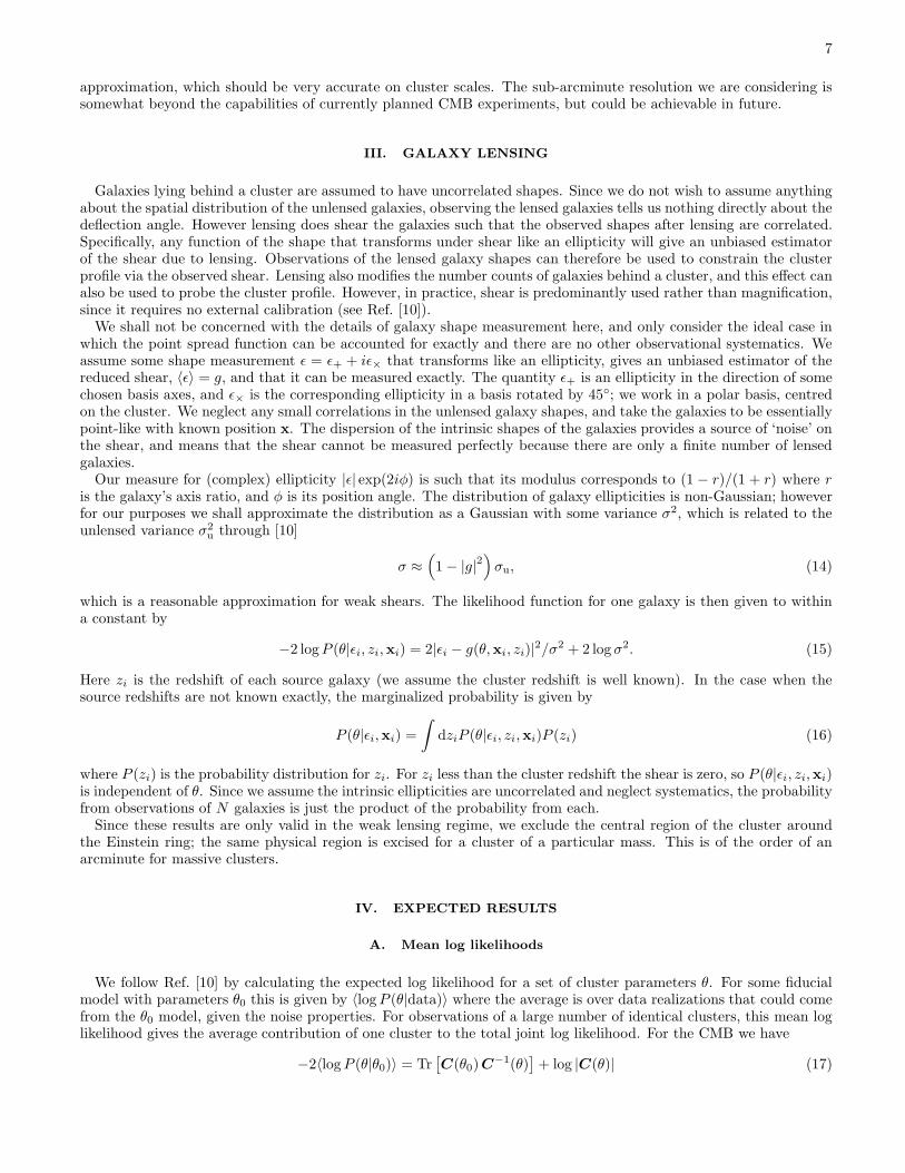
FIG. 1: Simulated effect of cluster lensing on the CMB temperature. Left: the unlensed CMB; middle: the lensed CMB; right:the difference due to the cluster lensing. The cluster is at z = 1, and has a spherically symmetric NFW profile with mass ofM200 = 1015h−1M⊙ and concentration parameter c = 5. Distances are in arcminutes, and can be compared to r200 = 3.3 arcmin.This is a rather clean realization; in general the dipole pattern can be weaker and/or more complicated. Note the inverteddirection of the gradient within the arcminute-scale Einstein radius in the middle figure.

II. CMB LENSING

A. CMB temperature lensing

The unlensed CMB is very smooth on small scales due to diffusion damping, so the small scale unlensed CMB canbe locally approximated as a gradient. Clusters act as converging lenses, making CMB photons appear to originatefurther from the centre of the cluster than they actually do. So the side of the cluster on the cold side of the gradientwill look hotter after lensing, and that on the hot side will look colder, giving a distinctive dipole-like signature alignedwith the direction of the background CMB gradient. The CMB lensing signature therefore consists of small scalewiggles in the observed temperature (and polarization) in an otherwise smooth background [12, 13, 14, 15, 16]. Aparticular example is shown in Fig. 1. Note that within the Einstein radius the lensing is not strictly weak (thoughdeflection angles remain small), however we shall include the signal everywhere as the strong lensing signal on theCMB is no more difficult to model than the weak signal in the single thin lens approximation that we use.For a Gaussian unlensed temperature field Θ, the temperature gradient variance is given by

〈|∇Θ|2〉 =∑

l

l(l+ 1)2l + 1

4πCΘ

l , (1)

where CΘl is the unlensed CMB temperature power spectrum. For typical ΛCDM models that we consider here the

rms is ∼ 14µK/arcmin. Since massive clusters can give deflections of the order of an arcminute, the signal is expectedto be at the ∼ 10µK level. The scale of the dipole-like pattern induced by the cluster lensing is much smaller than thescale of fluctuations in the unlensed CMB, and so should in principle easily be observable with high enough resolutionand low enough noise. However the signal depends on the background gradient, so only clusters in front of a significantgradient can have their mass constrained this way. The gradient at a point is a Gaussian random variable, so howoften this happens will depend on how sensitive the observations are to small signals and the level of complicatingsignals acting as sources of correlated noise.The observed direction of a point on the CMB last scattering surface is related to the direction it would have had

without lensing by a deflection angle α, determined in the small-angle Born approximation by

α(n) = −2

∫ χS

0

dχ

(

1− χ

χS

)

∇⊥Ψ(χn; η), (2)

where n is the direction of observation, χS is the comoving distance to the source at the last scattering surface (takento be thin), η is the time at which the photon was at position χn, and Ψ is the Newtonian potential. For clusterlensing the integral is dominated by the small part through the thin cluster and the angular factor 1 − χL/χS maybe taken out of the integral, where χL is the distance to the cluster. The potential is related to the comoving densityperturbation via the Poisson equation. For a more detailed review of CMB lensing see Ref. [17].If the background gradient could be measured cleanly away from the cluster, the cluster deflection angles could be

reconstructed directly, and hence used to solve for the cluster profile and mass given certain assumptions. Unfortu-nately the situation is more complicated because the unlensed CMB isn’t exactly a gradient — clusters have finite

3

angular size so the unlensed CMB in reality has more complicated spatial structure. There is also additional smallscale power due to other lensing sources along the line of sight, not to mention other important non-linear effects.Fortunately the problem is statistically straightforward if we take the unlensed CMB field to be Gaussian. For a givendeflection field the lensed CMB is also Gaussian since the deflections just re-map points: a uniform sampling of thelensed CMB just corresponds a non-uniform (and possibly multiple) sampling of the unlensed CMB. The correlationfunction of the observed temperature is therefore just given by the correlation function at the undeflected position onthe last scattering surface (neglecting complications due to other lensing along the line of sight). We can thereforework out the likelihood of any given cluster deflection field α(θ) for some set of cluster parameters θ using

−2 logP (α(θ)|Θ) = Θ(xi)C−1(xi,xj)Θ(xj) + log |C(xi,xj)|, (3)

where i, j index the different observed positions (taken here to be pixel centres) which are summed over implicitly inthe first term. Here C is given by the pixel noise covariance plus the covariance matrix determined by the correlationfunction of the unlensed temperature field Θ:

CΘ(x,x′) ≡ 〈Θ(x)Θ(x′)〉 = CΘ(β) =

∑

l

2l+ 1

4πCΘ

l Pl(cosβ), (4)

where β is the angular separation between x and x′. Here we only consider isotropic white (uncorrelated) noise σ2N (x)

so that

C(xi,xj) = CΘ(xi +αi,xj +αj) + δijσ2N (xi). (5)

Non-zero noise regularizes the inverse, for example the case when two observations on the Einstein ring are actuallysampling the same point on the last scattering surface. The effect of lensing by other perturbations along the line ofsight can be crudely modelled by using the lensed power spectrum, though a more careful analysis would require a studyof the non-Gaussian distribution numerically using simulations. We shall only consider small pixelized observations, inwhich case the dimension of the observed data vector is quite manageable, and the covariance matrix can be invertedexactly for each set of cluster model parameters considered. For discussion of beam issues see Section II C.Unfortunately the lensing cannot be observed directly, only its mixture with numerous other non-linear signals

including the Sunyaev-Zel’dovich (SZ) [1, 3, 5] and Rees-Sciama [18] effects. Thermal SZ is in principle not a problembecause of its distinctive spectral signature, and indeed could be used to help model the kinetic signal due to theircorrelated sources. Kinetic SZ is probably the most problematic [16], and has the same spectrum as the lensing signalwe are interested in. For a cluster that has circular symmetry about the line of sight, the kinetic SZ signal should alsohave circular symmetry, and therefore be orthogonal to the dipole-like lensing signal. However there will in generalbe non-symmetric spatially varying kinetic SZ both from cluster internal motion and other gas along the line of sightthat is more problematic. Cluster motion transverse to the line of sight can also give a kinetic Rees-Sciama signal,and secondary signals from outside the cluster can contribute additional sources of noise.We can easily include a known non-lensing secondary contribution Θm into the posterior distribution,

−2 logP (θ|Θtot,Θm) = (Θtot −Θm)†C−1(Θtot −Θm) + log |C|, (6)

where Θtot is the observed temperature (a sum of the lensing signal and other secondary signals). In general theother secondaries will also depend on the parameters θ and are hard to model.

Moving lens effect

If the cluster has a significant velocity transverse to the line of sight there will be a moving lens signal [17, 19, 20, 21]:a photon passing the front side of the lens (with respect to the direction of motion) will see a weaker potential onits way into the lens than on the way out, and hence receives a net redshift. Similarly a photon on the other sidewill receive a net blue shift. The moving lens therefore induces a dipole-like temperature anisotropy, which is at theµK level for massive clusters [21]. This is essentially the kinetic component of the Rees-Sciama effect (the nonlineargrowth component gives a small non-dipole-like effect that we neglect). The moving lens signal can also be viewedas dipole lensing: in the rest frame of the cluster, the cluster sees a CMB dipole; lensing deflects photons so thoseappearing to come from the front hot side actually come from closer to the cold side, and hence appear colder, andconversely on the other side.The moving lens dipole-like signal is easy to model [19, 22]. The temperature anisotropy induced by a small lens

moving perpendicular to the line of sight with velocity v⊥ (natural units) is at lowest order

∆Θ

Θ= −2

∫

dχv⊥ ·∇⊥Ψ(χn; η) = v⊥ · δβ, (7)

4

where δβ is the deflection angle of the photon at the lens (related to the observed deflection angle by α = (1 −χL/χ

∗)δβ). The moving lens signal therefore looks very similar to the dipole-like lensing signal, though unlikethe lensing signal the direction of the dipole pattern is determined by the velocity rather than the (uncorrelated)background CMB gradient. The moving lens signal is a source of confusion for the static lensing signal if there is noway to measure the transverse cluster velocity independently (e.g. using CMB polarization).If we model the cluster peculiar velocities as a 3-D Gaussian random field with rms velocity vrms, the transverse

velocity is also Gaussian with 〈v2⊥〉 = 〈v2x + v2y〉 = 2v2rms/3. Writing Θm = ∆Θ = Θδβ · v⊥ ≡ vxΘm,x + vyΘm,y we

then have

Cm ≡ 〈ΘtotΘtot†〉 = 〈ΘΘ† +ΘmΘ†m〉 = C +

v2rms

3

(

Θm,xΘ†m,x +Θm,yΘ

†m,y

)

. (8)

Here we have assumed any correlation between the CMB and velocity is negligible so the fields are uncorrelated.Marginalized over the transverse cluster velocity the likelihood is therefore

−2 logP (θ|Θtot) = Θtot†C

−1m Θtot + log |Cm|. (9)

Note that in general vrms is a function of the cluster parameters and redshift. The velocities of nearby clusters willalso be correlated to some extent, in which case treating the velocity uncertainty as independent Gaussians would notbe quite correct. We may also be interested to extract information about the transverse velocity, in which case thevelocity posterior distribution could be calculated rather than marginalizing over it as we do here.

Kinetic SZ from cluster rotation

In the ideal symmetric case adding a symmetric kinetic SZ template has no effect on parameter constraints becausethe affected modes are orthogonal to those sensitive to the dipole-like lensing signal. This is true even though thekinetic SZ is expected to have significantly larger amplitude. The extent to which asymmetric kinetic SZ confusesthe signal really needs to be tested from simulations [15, 16], which indicate that in practice it is a major source ofconfusion.1 Here we consider only a simple analytic model.A simple situation that can give a dipole-like kinetic SZ signature is when the cluster is rotating [24, 25]. We can

model this easily even in the idealized case following Ref. [25]. We assume the cluster is rigidly rotating inside thevirial radius, and that that the gas is in hydrostatic equilibrium in a non-rotating dark matter potential [26]. Thekinetic SZ temperature anisotropy is given by

∆Θ

Θ= σT

∫

dχnen · v, (10)

where the integral is along the line of sight in direction n, and the gas velocity is determined from the radius,mass and the cluster angular momentum, the latter being parameterized by the dimensionless parameter λ followingRefs. [25, 27]. The electron density ne is assumed to be associated with the fully ionized gas. We shall make thecrude approximation that the angular momenta have a 3-D Gaussian distribution, with λrms = 0.04 as in [25]. Thisrms value is broadly consistent with that found in simulations [27]. Assuming we have no knowledge of the clusterrotation, we can then marginalize over the kinetic SZ signal in exactly the same way that we did for the movinglens signal. The kinetic SZ signal from rotation gives a dipole-like pattern peaking at a few µK near the centre, butfalls off rapidly at large radii (well inside the virial radius). As for the moving lens signal the direction of the dipoleis expected to be uncorrelated with the background CMB gradient, and we assume it is also uncorrelated with thetransverse velocity.The components of the angular momentum transverse to the line of sight could be measured by other means, for

example from the redshifts of the galaxies, so in principle it may be possible to model this signal out. Howeverit is useful to consider it as an indicator of the level of problems caused by more general kinetic SZ signals fromsubstructure and internal motion.Since we wish to extract constraints from CMB lensing here rather than by modelling the (in reality complicated)

kinetic SZ, we shall take the fixed fiducial parameters when calculating the kinetic SZ contribution to the covariance.If the kinetic SZ could be modelled reliably as a function of cluster parameters then parameter constraints could beimproved.

1 Ref. [23] find a small effect from kinetic SZ, but they only consider the symmetric component.

5

Background secondaries

On scales l & 4000 the spectrum from inhomogeneous reionization and secondary doppler signals is expected to bevery roughly scale invariant with l(l+1)Cl/2π ∼ 5µK2 [28] and dominates the (cluster-free) lensed CMB power. Theextra power provided by this signal actually increases the rms temperature gradient behind the cluster significantly,which tends to increase the lensing signal. This is compensated by the increased smaller scale power, acting as asource of correlated noise, and degrading parameter constraints. Neglecting non-Gaussianity and the different redshiftof the source, it can be modelled simply by adding the approximately scale invariant power spectrum to the unlensedpower spectrum used for computing the unlensed covariance.In principle, discrete secondary sources behind the cluster will be sheared by the lens, so shear measurements can

be used to obtain additional information about the cluster [29]. This would require substantially higher resolutionobservations, and a detailed investigation is beyond the scope of this paper.

B. CMB polarization lensing

The CMB temperature cluster lensing signal is complicated by many sources of confusion, including sizeable kineticSZ and moving lens signals. The lensing signal is also small if the temperature gradient behind a cluster happensto be small. Furthermore any attempted density profile reconstruction will have degeneracies because the singletemperature gradient will not show up orthogonal deflection angles. In principle CMB polarization observations canhelp with all of these problems.The statistics of the polarization gradients is discussed in the appendix. The rms gradient of each Stokes’ parameter

is ∼ 1µK/arcmin, so a signal ∼ 1µK is expected for massive clusters. On cluster scales the correlation with thetemperature gradient is fairly small, at the 10% level, so the directions of the gradients are close to independent. Theaddition of polarization data is therefore very much like adding two new temperature fields but with lower signal andslightly different CMB ‘noise’ properties.The polarization signal is about a factor of ten lower than the temperature signal, so detection will be challenging.

However the polarization signal should be significantly cleaner as the other secondary polarization signals are generallysmall [30, 31, 32, 33, 34]. The dominant frequency-independent signal is expected to be from scattering of theprimordial CMB temperature quadrupole from ionized gas in the cluster. This depends linearly on the cluster opticaldepth (∼ 1%), and typically gives a signal . 0.1µK [35, 36, 37, 38]. This signal is strongly correlated across the skyfor clusters at similar redshifts due to the small variation of the quadrupole within a Hubble volume, and is also fairlyconstant across each cluster (in contrast to the lensing dipole-like signal). It may therefore be possible to subtract itout. For spherically symmetric clusters the signal should be orthogonal to the lensing signal and hence irrelevant, sowe shall neglect it here. There will however be hard to model spatial variations due to varying quadrupole and ionizedgas density within the cluster that prevent this being done perfectly, but we can expect residuals to be ≪ 0.1µK.The dominant frequency-dependent signal is likely to be re-scattering of anisotropic thermal SZ, giving a frequency-

dependent cluster polarization signal . 0.7µK [34, 39] at the peak of the SZ spectrum. Multi-frequency observationsshould be able to subtract this out, and lower frequency observations would in any case see significantly less signal.Polarization from scattering of the kinetic quadrupole is expected to be around ten times lower than the signal fromscattering of the primordial quadrupole [5, 31, 36], has a different frequency dependence, and should anyway beorthogonal to the lensing signal at lowest order. Contributions from cluster rotation are expected to be very small,∼ 10−4µK [24]. Other signals such as Faraday rotation also have a distinct spectral signature so in principle theycan be separated out using multi-frequency observations. The small scale signal from inhomogeneous reionizationis expected to be small [40, 41], and below the signal expected from other lenses. We shall simply assume that allnon-lensing signals can be removed or are negligible, and roughly model the small effect of other lenses along the lineof sight by using the lensed CMB polarization power spectra.The unlensed polarization fields are expected to be Gaussian, and the full polarized posterior can be computed as

for the temperature using the correlation functions between the Stokes’ parameters at the undeflected positions. Thepolarization field can be described as a complex spin two field P = Q + iU . The scalar correlation function betweenpolarization at x and x′ should be independent of the basis used to define P at the two points. To do this, we wantto describe the polarization in the physically relevant basis defined by r = x − x′. If r makes an angle φr to the exaxis, this amounts to rotating the basis by an angle φr anticlockwise at each point, giving Pr(x) = e−2iφrP (x). In

6

this physical basis we can then define the basis-independent correlation functions [42, 43]

ξ+(β) ≡ 〈Pr(x)∗Pr(x

′)〉 = 〈P (x)∗P (x′)〉 =∑

l′

2l + 1

4π(CE

l + CBl )dl22(β) (11)

ξ−(β) ≡ 〈Pr(x)Pr(x′)〉 = 〈e−4iφrP (x)P (x′)〉 =

∑

l

2l+ 1

4π(CE

l − CBl )dl2−2(β) (12)

ξX(β) ≡ 〈Θ(x)Pr(x′)〉 = 〈Θ(x)e−2iφrP (x′)〉 =

∑

l

2l+ 1

4πCX

l dl02(β). (13)

Here CEl and CB

l are the E-mode (gradient-like) and B-mode (curl-like) power spectra [44], and CXl is the cross

correlation of the E-modes with the temperature. The dlmn are the reduced Wigner functions (see e.g. Ref. [45]).Note that a pure polarization gradient is neither unambiguously E or B, as the decomposition is non-local anddepends on second derivatives. The decomposition into E- and B-modes is not especially helpful for analysing thecluster polarization signal: on cluster scales both the unlensed E- and B-mode power spectra are expected to besmall, with lensing introducing approximately equal small scale power into both (see the appendix). For Gaussianfields an optimal analysis can be performed using the Stokes parameters directly without decomposition into E- andB-modes.Writing the observed pixel temperature, Q and U as a combined vector (Θ,Q,U), these correlation functions are

sufficient to calculate the full covariance matrix that we need for computing the likelihood function given by theobvious generalization of Eq. (3). Since the temperature signal is likely to be complicated by secondary signals,we shall mostly consider the polarization measurements separately from the temperature, though including the fullcorrelation structure is no problem if required. Since the polarization signal is so much smaller than the temperature,any noise level that allows polarization detection will generally give a much better constraint from the temperatureif the temperature signal is clean enough. However in practice confusion with other secondaries may make thepolarization more useful at low noise levels.

C. Beam and pixelization

The effect of beam convolution is complicated because the beam convolves the lensed rather than unlensed sky. Aneffectively circular Gaussian beam will in general measure a non-circular non-Gaussian average of the unlensed skydue to the non-uniform lensing field. If the unlensed sky and deflection angle over a pixel can be well approximatedby a gradient, a pixel (or pixel-size beam) average will be very close to the value at the pixel centre, which is what weuse here. However inside the Einstein radius the deflection angle gradient can change significantly on the pixel scale,and a more careful analysis would be required for very accurate results.If the centre of a circular pixel is aligned with the centre of a spherically symmetric cluster, an integral over the

pixel should give the same as the value at the centre of the pixel, which should be the same as the unlensed value.In this case the pixel gives essentially no information about the cluster. However if the grid of pixels is offset fromthe centre of the cluster, two adjacent central pixels will have different signals and slightly more information can begained about the central cluster profile. This manifests itself as a somewhat better upper limit on the concentrationparameter c when pixels centres are offset. Since a generic observation will not be aligned exactly with the clusterwe have chosen to offset our pixels so as not to introduce artificial symmetries. However there is some error fromusing the values at the centre of the pixels. We find that for the basic case the results are fairly insensitive to thepixel integration (checked explicitly by calculating the covariance for pixel values taken to be an average of 4 or9 sub-pixels). The behaviour is more complicated when there is significant small scale unlensed power, eg. frominhomogeneous reionization. We do not attempt to model the beam effect in detail here. When small scale unlensedpower is included our results should be taken as an approximate estimate; a more detailed analysis would be neededfor any given actual experimental beam. For distant clusters with masses ∼ 2× 1014M⊙ the Einstein radius is around0.2 arcmin, which for aligned pixels would lie entirely within a central pixel of side 0.5 arcmin. In this case the resultfrom using aligned pixels (where the central pixel contributes no information) should give an idea of the result whenthe strong lensing region is ignored, which corresponds to somewhat increasing the upper limit on c compared to theresults we present using all the (offset) pixels.The effect of pixel (beam) size and cluster redshift is explored in detail in Ref. [14]. Here we shall fix the pixel

size to 0.5 arcmin, and use a square box of side 8 arcmin (16 pixels) nearly centred over the cluster. Due to the smallscale power in the CMB, using larger box sizes gains very little since the cluster signature cannot be distinguishedfrom variations in the primordial CMB, and our results are stable to increasing the box size. We use the flat sky

7

approximation, which should be very accurate on cluster scales. The sub-arcminute resolution we are considering issomewhat beyond the capabilities of currently planned CMB experiments, but could be achievable in future.

III. GALAXY LENSING

Galaxies lying behind a cluster are assumed to have uncorrelated shapes. Since we do not wish to assume anythingabout the spatial distribution of the unlensed galaxies, observing the lensed galaxies tells us nothing directly about thedeflection angle. However lensing does shear the galaxies such that the observed shapes after lensing are correlated.Specifically, any function of the shape that transforms under shear like an ellipticity will give an unbiased estimatorof the shear due to lensing. Observations of the lensed galaxy shapes can therefore be used to constrain the clusterprofile via the observed shear. Lensing also modifies the number counts of galaxies behind a cluster, and this effect canalso be used to probe the cluster profile. However, in practice, shear is predominantly used rather than magnification,since it requires no external calibration (see Ref. [10]).We shall not be concerned with the details of galaxy shape measurement here, and only consider the ideal case in

which the point spread function can be accounted for exactly and there are no other observational systematics. Weassume some shape measurement ǫ = ǫ+ + iǫ× that transforms like an ellipticity, gives an unbiased estimator of thereduced shear, 〈ǫ〉 = g, and that it can be measured exactly. The quantity ǫ+ is an ellipticity in the direction of somechosen basis axes, and ǫ× is the corresponding ellipticity in a basis rotated by 45; we work in a polar basis, centredon the cluster. We neglect any small correlations in the unlensed galaxy shapes, and take the galaxies to be essentiallypoint-like with known position x. The dispersion of the intrinsic shapes of the galaxies provides a source of ‘noise’ onthe shear, and means that the shear cannot be measured perfectly because there are only a finite number of lensedgalaxies.Our measure for (complex) ellipticity |ǫ| exp(2iφ) is such that its modulus corresponds to (1 − r)/(1 + r) where r

is the galaxy’s axis ratio, and φ is its position angle. The distribution of galaxy ellipticities is non-Gaussian; howeverfor our purposes we shall approximate the distribution as a Gaussian with some variance σ2, which is related to theunlensed variance σ2

u through [10]

σ ≈(

1− |g|2)

σu, (14)

which is a reasonable approximation for weak shears. The likelihood function for one galaxy is then given to withina constant by

−2 logP (θ|ǫi, zi,xi) = 2|ǫi − g(θ,xi, zi)|2/σ2 + 2 log σ2. (15)

Here zi is the redshift of each source galaxy (we assume the cluster redshift is well known). In the case when thesource redshifts are not known exactly, the marginalized probability is given by

P (θ|ǫi,xi) =

∫

dziP (θ|ǫi, zi,xi)P (zi) (16)

where P (zi) is the probability distribution for zi. For zi less than the cluster redshift the shear is zero, so P (θ|ǫi, zi,xi)is independent of θ. Since we assume the intrinsic ellipticities are uncorrelated and neglect systematics, the probabilityfrom observations of N galaxies is just the product of the probability from each.Since these results are only valid in the weak lensing regime, we exclude the central region of the cluster around

the Einstein ring; the same physical region is excised for a cluster of a particular mass. This is of the order of anarcminute for massive clusters.

IV. EXPECTED RESULTS

A. Mean log likelihoods

We follow Ref. [10] by calculating the expected log likelihood for a set of cluster parameters θ. For some fiducialmodel with parameters θ0 this is given by 〈logP (θ|data)〉 where the average is over data realizations that could comefrom the θ0 model, given the noise properties. For observations of a large number of identical clusters, this mean loglikelihood gives the average contribution of one cluster to the total joint log likelihood. For the CMB we have

−2〈logP (θ|θ0)〉 = Tr[

C(θ0)C−1(θ)

]

+ log |C(θ)| (17)

8

where C(θ) is the correlation matrix for the undeflected points. The mean log likelihood peaks at the true modelθ = θ0, and the shape of the likelihood contours give a good idea of the degeneracy directions expected from particularobservations. For the temperature case C is replaced with Cm when we want to marginalize over the moving lens orrotating SZ signals.The mean log likelihood for one galaxy at redshift z is [10]

− 2〈logP (θ|θ0,x, z)〉 = −2

∫

d2ǫP (ǫ|θ0) logP (θ|ǫ, z,x)

= 2

( |g(θ,x, z)− g(θ0,x, z)|2 + σ20

σ2+ log σ2

)

, (18)

where σ0 denotes σ (g (θ0)). Given the probability P (N) to find N galaxies in the data field (which follows a Poissondistribution and is independent of position) the number density observed n(θ0,x, z) depends on the magnification dueto the lensing. We follow Ref. [10] by taking the scaling of number density with magnification µ to be [µ(θ0,x, z)]

β−1,where β is the slope of the unlensed number counts, taken to be 0.5. The number density function averaged over thetotal number density distribution is then

〈n(θ0,x, z)〉N =

∫

dN [µ(θ0,x, z)]β−1NP (N)P (z) = nγ [µ(θ0,x, z)]

β−1P (z), (19)

where nγ is the expected unlensed angular number density (including all redshifts) for which a shape can be measured.The source galaxies have a redshift probability distribution P (z) normalized so

∫∞

0 dzP (z) = 1. The total mean loglikelihood is then

− 2〈logP (θ|θ0)〉 = −2

∫

dz

∫

d2x 〈n(θ0,x, z)〉N 〈logP (θ|θ0,x, z)〉ǫ

= 2nγ

∫

dzP (z)

∫

d2x[µ(θ0,x, z)]β−1

( |g(θ,x, z)− g(θ0,x, z)|2 + σ20

σ2+ log σ2

)

(20)

as derived in Ref. [10]. Monte Carlo simulations were also performed in Ref. [10] which showed that the scatterof maximum likelihood points in different realizations corresponds well with the mean log likelihood contours. Forgalaxies with redshift less than the cluster the shear is zero, and there is no contribution to the integral (except anirrelevant constant). This result is valid when the observations measure the redshift of each galaxy accurately. In thecase when the redshifts are uncertain the result is more complicated

− 2〈logP (θ|θ0)〉 = −2

∫

dz

∫

d2x 〈n(θ0,x, z)〉N 〈logP (θ|θ0,x)〉ǫ

= −2nγ

∫

dzP (z)

∫

d2x [µ(θ0,x, z)]β−1

∫

d2ǫ P (ǫ|θ0, z,x) log[∫

dz′P (θ|ǫ, z′,x)P (z′|z)]

,(21)

which cannot easily be simplified any further. Here P (z′|z) is the post-observation distribution of the redshift z′ giventhe galaxy is actually at z. Note that Eq. (20) reduces to Eq. (19) when the source redshifts are known.Throughout we shall assume a purely adiabatic standard ΛCDM cosmology with Hubble parameter H0 =

70 kms−1Mpc−1, dark matter density Ωch2 = 0.11, baryon density Ωbh

2 = 0.022, spectral index ns = 0.99, pri-mordial curvature perturbation amplitude As = 2.5 × 10−9 (corresponding to matter fluctuation parameter todayσ8 ≈ 0.87) and optical depth τ = 0.15.

B. Spherically symmetric NFW clusters

Our main purpose here is to compare the power of different sources for cluster mass lensing reconstruction. Wetherefore use a simple parameterization for the cluster radial profile, and see how well the parameters can be con-strained using different methods. We shall follow Ref. [14] and assume clusters with a spherically symmetric NFWprofile [46] given by

ρ(r) =A

r(cr + r200)2(22)

9

for some concentration parameter c, and radius r200. We shall parameterize the mass of the cluster by that inside theradius r200 defined so that it is 200 times the mean density of a critical density universe at the cluster redshift,

M200 ≡ 2004π

3ρc(z)r

3200, (23)

where ρc(z) is the critical density at the redshift of the cluster, 3H2(z)/8πG. The amplitude is given in terms of themass and concentration parameter by

A =M200c

2

4π[ln(1 + c)− c/(1 + c)]. (24)

The deflection at the cluster is then given by [14]

δβ(r) =−16πGA

c2 rsF (r/rs)r, (25)

where r is the transverse distance from the centre of the cluster, r ≡ r/r, rs ≡ r200/c is the scale radius, and

F (x < 1) =1

x

(

ln(x/2) +ln(x/[1−

√1− x2])√

1− x2

)

F (x = 1) = 1− ln(2) (26)

F (x > 1) =1

x

(

ln(x/2) +π/2− sin−1(1/x)√

x2 − 1

)

.

The observed deflection is then given by δθ = (1−χL/χS)δβ where χL and χS are the comoving distances to the lensand the source (for the CMB taken to be the point of maximum visibility on the last scattering surface).The convergence κ is (minus one half) the angular divergence of the observed deflection angle, and at the radial

distance r from the centre of the cluster is given by (see e.g. Ref. [47])

κ(r) = κkf(r/rs) , (27)

where f(x) = x−1 ddx [xF (x)] is

f(x < 1) =1

x2 − 1

(

1− 2 tanh−1√

(1 − x)/(1 + x)√1− x2

)

f(x = 1) =1

3(28)

f(x > 1) =1

x2 − 1

(

1− 2 tan−1√

(x− 1)/(x+ 1)√x2 − 1

)

.

Here

κk ≡ 2rsρsΣcrit

=8πGA

c2r2sDL(1 − χL/χS), (29)

where Σcrit = [4πGDL(1 − χL/χS)]−1 is the (redshift dependent) critical surface mass density of the lens and the

angular diameter distance to the lens is DL. The characteristic density of the halo ρs is related to the amplitude Athrough

ρs =Ac

r3200. (30)

In a polar basis centred on the cluster the shear γ is real and given by

γ(r) = κkj(r/rs) , (31)

10

z = 2

2

4

6

8

10

12

14

16z = 1

z = 0.5

0.5 1 1.5

2

4

6

8

10

12

14

16z = 0.25

0.5 1 1.5 2PSfrag replacements

M200/1015h−1M⊙M200/1015h−1M⊙

cc

FIG. 2: Mean log likelihood constraints for a M200 = 1015h−1M⊙ cluster with concentration parameter c = 5 using CMBtemperature lensing only. Dark solid is CMB lensing for 1µK noise per 0.5 arcmin pixel assuming only lensing signal, palersolid is when a moving lens contribution is added and constraints are marginalized assuming a Gaussian velocity distributionwith vrms = 300 kms−1. Dashed lines show the constraints marginalized over an unknown rotating kinetic SZ contribution.Contours show where the exponential of the mean log likelihood drops to 0.32 and 0.05 of the maximum.

where

j(x < 1) =4 tanh−1

√

(1− x)/(1 + x)

x2√1− x2

+2 ln

(

x2

)

x2− 1

x2 − 1

2 tanh−1√

(1 − x)/(1 + x)

(x2 − 1)√1− x2

j(x = 1) = 2 ln

(

1

2

)

+5

3(32)

j(x > 1) =4 tan−1

√

(x− 1)/(x+ 1)

x2√x2 − 1

+2 ln

(

x2

)

x2− 1

x2 − 1+

2 tan−1√

(x− 1)/(x+ 1)

(x2 − 1)3

2

.

The reduced shear g follows from g = γ/(1− κ) and the magnification µ = 1/(

(1− κ)2 − |γ|2)

.

C. CMB lensing

The parameters we shall attempt to constrain are the concentration c and the mass parameterized by M200. Forsimplicity we shall assume the position of the centre is known (for example from observations of the thermal SZ), sothere are only two parameters.Since our model is spherically symmetric the kinetic SZ from line of sight motion is also symmetric about the

cluster centre, and therefore orthogonal to the lensing signal. It can therefore be neglected. We show the effect ofmarginalizing over the various asymmetric signals on massive cluster constraints in Fig. 2. As a rough model of the

11

z = 2

5

10

15

20

25

z = 1

z = 0.5

0.1 0.2 0.3 0.4

5

10

15

20 z = 0.25

0.1 0.2 0.3 0.4 0.5PSfrag replacements

M200/1015h−1M⊙M200/1015h−1M⊙

cc

FIG. 3: Mean log likelihood constraints for a M200 = 2× 1014h−1M⊙ cluster with concentration parameter c = 5 using CMBlensing only with noise 0.1µK per 0.5 arcmin pixel. Filled contours are for temperature lensing, from the inside out (dark tolight) they are: 1. CMB lensing only; 2. Marginalized over moving lens signal; 3. Marginalized over moving lens signal andincluding small scale power from inhomogeneous reionization. The dashed line shows the result when the kinetic SZ signalfrom cluster rotation is unknown and also marginalized. The solid unfilled contour shows the result from a clean polarizationobservation with noise

√2 × 0.1µK on each Stokes’ parameter. Contours enclose the area where the exponential of the mean

log likelihood is greater than 0.05 of the peak value.

moving lens signal we take a constant vrms = 300 kms−1 (see e.g. Ref. [48]). Although only a fairly small effect atlow redshift where the constraints are weak anyway, at high redshift the moving lens signal significantly increases theuncertainty in the cluster mass. Kinetic SZ from cluster rotation is a big problem if this cannot be modelled, andreflects the fact that temperature mass measurements are probably kinetic SZ limited [15, 16]. At the 0.5µKarcminnoise level the polarization does not give a useful constraint due to the polarization signal being about ten timessmaller than the temperature.At high redshift there are expected to be almost no very massive clusters, so in Fig. 3 we show the effect for a

more realistic cluster with M200 = 2× 1014h−1M⊙ with ten times lower noise, 0.05µKarcmin (√2× 0.05µKarcmin

on the Stokes’ parameters). In the absence of confusing signals the temperature CMB gives excellent constraints athigh redshift. However these are massively degraded by marginalization over other non-linear effects. The effect ofmore small scale power from inhomogeneous reionization significantly degrades the constraints at low redshift. Wealso show the constraint expected from a clean polarization observation, which at this noise level is competitive withwhat can realistically be achieved from the temperature.

12

z = 0.25

0.5 1 1.5

2

4

6

8

10

12

14

16

18

z = 0.5

0.5 1 1.5 2PSfrag replacements

M200/1015h−1M⊙M200/1015h−1M⊙

c

FIG. 4: Mean log likelihood constraints for a M200 = 1015h−1M⊙ cluster with concentration parameter c = 5 from galaxylensing with 30 galaxies arcmin−2 and an intrinsic ellipticity dispersion σu = 0.3. Solid contours show the constraint for 〈z〉 = 1when galaxy redshifts are known, dashed is the equivalent result when the redshift distribution is known. Contours show wherethe exponential of the mean log likelihood drops to 0.32 and 0.05 of the maximum.

z = 2

5

10

15

20

25

z = 1

z = 0.5

0.5 1 1.5 2

5

10

15

20

z = 0.25

0.5 1 1.5 2PSfrag replacements

M200/1015h−1M⊙M200/1015h−1M⊙

cc

FIG. 5: Mean log likelihood constraints for a M200 = 1015h−1M⊙ cluster with concentration parameter c = 5. Dark solid isCMB lensing for 1µK noise per 0.5arcmin pixel marginalized over the moving lens signal, red solid is for space-based galaxylensing with 100 galaxies arcmin−2, dashed lines are for current ground-based galaxy lensing with 30 galaxies arcmin−2. Allgalaxies have known redshifts, σu = 0.3, and their distribution has 〈z〉 = 1. Contours show where the exponential of the meanlog likelihood drops to 0.32 and 0.05 of the maximum.

13

z = 2

5

10

15

20

25

z = 1

z = 0.5

0.1 0.2 0.3 0.4

5

10

15

20 z = 0.25

0.1 0.2 0.3 0.4 0.5PSfrag replacements

M200/1015h−1M⊙M200/1015h−1M⊙

cc

FIG. 6: Futuristic mean log likelihood constraints for a M200 = 2 × 1014h−1M⊙ cluster with concentration parameter c = 5.Dark solid is for clean CMB polarization lensing for

√2 × 0.1µK noise per 0.5arcmin pixel on the Stokes’ parameters, paler

solid is for galaxy lensing with perfect redshift information and a total of 500 galaxies arcmin−2 with a Gaussian ellipticitydistribution. All galaxies have σu = 0.2 and the distribution has 〈z〉 = 1.5. Contours show where the exponential of the meanlog likelihood drops to 0.32 and 0.05 of the maximum.

D. Galaxy lensing

We assume that the sources are randomly distributed on the sky, and have a redshift probability distribution P (z)dzof the form suggested by Ref. [49]

P (z)dz =η z2 exp [− (z/z0)

η]

Γ(

3η

)

z30

dz . (33)

Choosing P (z)dz = (27/2)z2 exp [−3z] dz gives 〈z〉 = 1, which is typical of current deep surveys. For comparison, wealso consider a survey with 〈z〉 = 1.5, the form of which is P (z)dz = 9.57z2 exp

[

−2.91z0.78]

dz. The distributions areskewed and peak at z = 2/3 and z ≈ 0.85 respectively.For clusters with z . 0.3, and for typical (current) weak lensing observations with 〈z〉 = 1, the cluster’s lensing

properties are quite insensitive to the actual redshift distribution of galaxies. The faint galaxy population can besafely approximated as lying on a sheet at 〈z〉, or more precisely at the redshift corresponding to 〈1/Σcrit(z)〉, withΣcrit(z) being the critical surface mass density. We do not however make this approximation here. The availabilityof photometric redshifts for galaxies is becoming increasingly likely with the advent of wide-field infrared imagers tocomplement observations from optical instruments, and parameter estimates from such data sets would be comparableto those with spectroscopic redshifts [11]. When there is no direct information about redshift, the galaxy’s magnitudecan be used to determine whether it is likely to be behind the cluster, so P (z′|z) ∼ P (z′) for z′ larger than about thecluster redshift, and small or zero otherwise.For the M200 = 2 × 1014h−1M⊙ cluster, the minimum radius of the aperture from which data is assumed to be

14

available is 0.145Mpc, and for the M200 = 1015h−1M⊙ cluster it is 0.35Mpc. For the outer radius, we integrate untilthe shear signal is negligible, and convergence in constraints is obtained. For the most massive cluster at z = 0.25,this is equivalent to an angular scale of ∼ 15 arcmin (or to that of a wide-field imager such as that on the ESO-MPG2.2m telescope).Fig. 4 shows expected constraints on massive cluster parameters from galaxy lensing with present day parameters.

The constraints on clusters with z & 1 are very weak with current data, so we show only the useful constraints forlower redshift clusters. The figure shows the degrading effect of not knowing the source galaxy redshifts which havebeen marginalized over using Eq. 21: for the z = 0.5 cluster this is a noticeable effect, however for z = 0.25 mostof the galaxies lie well behind the cluster so knowing the individual redshifts gains very little. At higher redshiftsthe effect would be much more important, however future surveys able to give a useful constraint for higher redshiftclusters would almost always have redshift information anyway.In Fig. 5 we compare current galaxy lensing constraints to those from possible future CMB temperature lensing

observations. Even current galaxy lensing data can do better than futuristic CMB temperature lensing for low redshiftclusters. However for z & 0.5 CMB lensing would be able to improve on current constraints if asymmetric kinetic SZcontamination and background secondaries did not destroy the signal. The fact that the CMB lensing constraints areweaker at low redshift when the deflection angle is larger may seem odd. However the point is that the deflection itselfis unobservable, only the dipole-like variation can be cleanly distinguished from variations in the unlensed CMB. Theconstraints are therefore better for higher redshift clusters where the cluster has a smaller angular size, and hence thedipole-like pattern is more easily distinguished from larger scale variations in the unlensed CMB.If Fig. 6 we compare futuristic constraints from clean CMB polarization lensing with constraints from futuristic

galaxy lensing with 〈z〉 = 1.5 (CMB polarization and temperature are compared in Fig. 3). For clusters with redshiftswell below the galaxy distribution peak, galaxy lensing should be much more powerful than CMB lensing. At redshiftshigher than the peak of the galaxy distribution function, the galaxy lensing results however become much worse dueto the lack of sources, and CMB polarization lensing may be a better way to measure the mass of clusters at redshiftz & 1. At these redshifts the CMB lensing result is also less degenerate with the concentration parameter than at lowredshift.Another source of noise in the determination of cluster mass profiles from galaxy lensing that we have neglected is

the large scale structure along the line of sight. This has been estimated to cause as much as a factor of 2 increase inuncertainties in estimates of c and M200 [50]. Structure correlated with a cluster leads to a bias, with the masses ofclusters in excess of 1014h−1M⊙ being overestimated by about 20% [51]. Techniques are being developed to alleviatethese issues (e.g. see Ref. [52]). For a particular cluster, if photometric or spectroscopic redshift information is availablefor the data field, then to some extent the importance of the large scale structure can be assessed by identifying anystructures (e.g. galaxy groups) along the line of sight, or correlated large scale structure such as filaments.

E. CMB lensing with non-symmetric profiles

So far we have presented results for mean log likelihoods that give an idea of average results per cluster when youobserve many. However one must remember that CMB temperature lensing constraint is highly variable due to thevariability of the gradient behind any given cluster. If a cluster happens to be in the middle of a broad hot spot therewill be essentially no constraint.The assumption of spherical cluster symmetry is also qualitatively important for the CMB temperature lensing

results. If a cluster is observed in front of a pure gradient field, then deflection in the direction orthogonal to thegradient will be unconstrained. If we assume spherical symmetry this does not really matter as the profile can beconstrained from the gradient-direction deflections. However if the cluster is non-symmetric, there is a fundamentaldegeneracy: CMB lensing of a pure gradient field cannot constrain orthogonal deflections at all. Of course the CMBis not a pure gradient, and in this case small scale CMB power actually helps to break this degeneracy to some extent.Furthermore CMB polarization provides two additional gradient directions, so the probability of all three gradientsbeing aligned or very small is low. Polarization observations should be able to significantly help general cluster profilereconstruction. This is important because in reality the majority of clusters are expected to be prolate [2] rather thanspherical, as well as having interesting substructure.General cluster profile reconstruction from CMB lensing is beyond the scope of this paper (see Ref. [23] for some

work with CMB temperature). Here we consider a simple toy model to illustrate the issues: we try to reconstruct astretched NFW deflection field

α = ζn · αNFW n+ n⊥ · αNFW n⊥ (34)

where ζ is a stretch parameter. We choose n to be in the direction of the CMB temperature gradient or the directionorthogonal to it, where n⊥ is the corresponding orthogonal direction. For simplicity we fix the concentration parameter

15

0.2

0.4

0.6

0.8

1

1.2

1.4

1.6

1.8

2

0.1 0.2 0.3 0.4

0.2

0.4

0.6

0.8

1

1.2

1.4

1.6

1.8

0.1 0.2 0.3 0.4 0.5PSfrag replacements

M200/1015h−1M⊙M200/1015h−1M⊙

ζζ

0.2

0.4

0.6

0.8

1

1.2

1.4

1.6

1.8

2

0.1 0.2 0.3 0.4

0.2

0.4

0.6

0.8

1

1.2

1.4

1.6

1.8

0.1 0.2 0.3 0.4 0.5PSfrag replacements

M200/1015h−1M⊙M200/1015h−1M⊙

ζζ

FIG. 7: Constraints on the stretch parameter ζ from four random realizations, for direction parallel (left) and orthogonal(right) to the direction of the background CMB temperature gradient. Solid lines are using CMB temperature only, dashedpolarization only, filled contours show the combined result (accounting for the correlation). The fiducial cluster was at redshiftone and has a spherically symmetric NFW profile with mass of M200 = 2 × 1014h−1M⊙. The noise is 0.1µK per 0.5 arcminpixel (

√2× 0.1µK for the polarization) the concentration is fixed to c = 5.

to c = 5, and only consider the idealized case where the temperature signal is purely CMB lensing. Note that thistoy model is not a realistic lensing deflection angle field as in general it is not curl free.In Fig. 7 we show the constraints on the stretch in the two orthogonal directions for four different realizations of

the underlying fields. The CMB temperature stretch constraint in the direction orthogonal to the CMB gradient isgenerally very poor. The CMB polarization constraints are slightly correlated, but generally in significantly differentdirections, meaning that joint constraints are significantly better than those from the CMB temperature alone.The presence of smaller scale CMB power from e.g. inhomogeneous reionization can actually improve the constraints

from the temperature in the orthogonal direction due to the extra information available in the smaller scale power.However, as emphasised above, the CMB temperature signal is likely to be complicated due to SZ etc, so in practicethe CMB temperature result is likely to be very much worse than that shown here. CMB polarization may be a muchbetter probe.

V. CONCLUSIONS

Weak lensing is a valuable and promising method for studying cluster masses. Measurements of lensing shear usingobservations of lensed galaxies provides tight constraints for low redshift clusters. For clusters at higher redshift thanthe peak of the galaxy-redshift distribution the galaxy lensing constraints become much poorer, and CMB lensing cando better. However, even with simple spherically symmetric models the temperature lensing signal can be degradedby various other second order effects. For futuristic arcminute-resolution observations at low noise levels the CMBpolarization lensing signal may be much cleaner and a more robust way to measure cluster properties. Measurementsof lensing by high redshift clusters is therefore something that future CMB polarization missions may wish to aim toachieve.The results from galaxy lensing are limited by the intrinsic ellipticity dispersion of the galaxies, and the fact that

there are only a finite number of sources behind the cluster. To do better one could try to find sources which havea higher number density. Possibilities include high redshift sources observed with 21cm, sources from the time ofinhomogeneous reionization, and secondary doppler CMB signals from velocities after reionization [29, 53, 54]. Inaddition strong lensing can be used to help constrain the central region of the cluster profile. The ultimate limitfrom CMB polarization will depend on how efficiently spectral information can be used to clean out confusing signals,and the extent to which cluster substructure complicates the signal from quadrupole scattering. Future work could

16

investigate this using numerical simulations.With the appropriate increase in resolution and sensitivity, methods for cluster CMB lensing could be extended to

constrain galaxy profiles (as discussed for the CMB temperature in Ref. [55]).

VI. ACKNOWLEDGMENTS

We thank Anthony Challinor, Jochen Weller for helpful suggestions, also Peter Schneider and Richard Battye. Wethank CITA for use of their Beowulf computer. AL acknowledges support via a PPARC Advanced Fellowship. LJKthanks the Royal Society for support via a University Research Fellowship.

APPENDIX A: GRADIENT APPROXIMATION

Since gradients are just linear combinations of the (assumed) Gaussian underlying fields, the gradient fields are alsoGaussian and hence fully described by their covariance. We can either work out the full distribution of the gradientsdirectly, or just work out the covariances. Here we chose to do the latter, and calculate the covariances of the gradientsat a point assuming statistical isotropy. The temperature gradient variance is given by

2PΘ ≡ 〈|∇Θ|2〉 = 〈∣

∣

∑

lm

Θlm∇Ylm

∣

∣

2〉

= −∑

l

CΘl

1

4π

∑

m

∫

dΩYlm∇2Y ∗lm

=∑

l

l(l+ 1)2l + 1

4πCΘ

l , (A1)

where we used statistical isotropy and orthogonality of the spherical harmonics. A polarization tensor Pab can bedefined so that in a fixed orthonormal basis

Pij =1

2

(

Q UU −Q

)

, (A2)

and may be expanded in terms of gradient and curl tensor spherical harmonics [56] Y Gab (lm) and Y C

ab (lm). The har-monic components describe the E- and B-modes of the polarization respectively. The correlation of the polarizationdivergence and temperature is given by

PX ≡ 1

2〈∇aPab∇bT 〉 =

1

2√2

∑

lm

CXl

1

4π

∫

∇aY Gab (lm)∇bY ∗

lm

= −1

4

∑

l

√

(l + 2)!

(l − 2)!

2l+ 1

4πCX

l , (A3)

where CXl is the temperature-polarization cross-correlation power spectrum. The other terms are zero:

〈∇aPab ǫbc∇cΘ〉 = 0. (A4)

The variance of the polarization divergence is

PP ≡ 〈∇aPab∇cPcb〉 = 1

4

∑

l

(l + 2)(l − 1)2l+ 1

4π(CE

l + CBl ). (A5)

Similar results can be derived for the variance of the irreducible polarization gradient 3-tensor. In terms of a fixedflat-sky basis we have

〈∇xU∇yΘ〉 = 〈∇yU∇xΘ〉 = 〈∇xQ∇xΘ〉 = −〈∇yQ∇yΘ〉 = PX , (A6)

〈|∇Q|2〉 = 〈|∇U |2〉 = 2PP , (A7)

17

with other terms being zero, as can readily be verified by using an explicit flat-sky harmonic expansion. The stochasticquantities are (∇xΘ,∇yΘ,∇xQ,∇yQ,∇xU,∇yU), which therefore have covariance

PT 0 PX 0 0 PX

0 PT 0 PX −PX 0PX 0 PP 0 0 00 PX 0 PP 0 00 −PX 0 0 PP 0PX 0 0 0 0 PP

. (A8)

The correlation PX is negative, and the (anti-)correlation PX/(PΘPP )1/2 is about 10%. On the small scales we are

considering, photons are flowing into hot spots, which for a plane wave means that the correlated part of Q (definedwith respect to the wavevector—parallel to ∇Θ—basis direction) is negative on the the hot crest [57]. Q thereforeincreases in the direction of the cold crest, and hence that the gradients in Q and Θ are anti-correlated. Note for ourconventions we have to flip sign of CX

l from CAMB/CMBFAST which use the conventions of Ref. [44].In a fixed flat sky basis, using the gradient approximation, some deflection field α(r) gives the lensed polarization

field

Pab(r) = Pab(r) +α(r) ·∇Pab. (A9)

A constant gradient is neither E or B-mode, because making the E/B decomposition locally requires taking twogradients. This is reflected in the fact that the covariance is a function only of the sum of the power spectra CE

l +CBl .

On the flat sky the scalar harmonics are eil·x and tensor harmonics are (we follow the conventions of Ref. [17])

QGab(l) = −

√2 l〈alb〉e

il·x (A10)

QCab(l) = −

√2 ǫc(a lb) lce

il·x, (A11)

where angle brackets denote the symmetric trace free part of the enclosed indices and l = l/|l|. Assuming a suitablywell behaved deflection field the lensed harmonic components are then

E(l) = −2α(l) ·∇Pab l〈a lb〉

B(l) = −2α(l) ·∇Pab ǫc(a lb)lc. (A12)

Averaging over (assumed Gaussian) background polarization gradients ∇Pab we get

〈|E(l)|2〉 = PP |α(l)|2

〈|B(l)|2〉 = PP |α(l)|2. (A13)

An arbitrary deflection field therefore gives identical power for each E and B mode on average when lensing a puregradient field. If the deflection field has circular symmetry (as from a spherical cluster), the angular average of the Eand B mode power are equal for any fixed polarization gradient:

1

2π

∫

dφl|E(l)|2 =α2(l)

4

(

|∇Q|2 + |∇U |2)

1

2π

∫

dφl|B(l)|2 =α2(l)

4

(

|∇Q|2 + |∇U |2)

. (A14)

Cluster lensing therefore generates equal amplitude E and B in the gradient approximation. However there is verylittle power in the unlensed E or B polarization on cluster scales, so the lensed E contains almost as much informationas the lensed B. We use the full likelihood function so there is in fact no need to use E and B. However for nearbylarge clusters the B mode signal may allow the cluster signal to be distinguished from unlensed CMB ‘noise’, so unlikein the temperature case cluster lensing may not be CMB noise limited for large cluster sizes.Since the temperature gradient defines a direction, we could chose to define the Q and U Stokes’ parameters with

respect to this variable basis, e.g. where we align the x-axis with ∇Θ. In this basis

〈|∇xΘ|2〉′ = 〈|∇Θ|2〉 = 2〈|∇xΘ|2〉, (A15)

18

simply twice the variance of the x-component in a fixed basis, and similar results hold for the non-zero terms.By choosing this basis we are however making the whole distribution non-Gaussian, for example the marginalizeddistribution of δ ≡ (∇xΘ)′ = |∇Θ| is P (δ) ∝ δ exp(−δ2/2PT ).

[1] M. Birkinshaw, Phys. Rept. 310, 97 (1999), astro-ph/9808050.[2] L. Shaw, J. Weller, J. P. Ostriker, and P. Bode (2005), astro-ph/0509856.[3] R. A. Battye and J. Weller, Phys. Rev. D68, 083506 (2003), astro-ph/0305568.[4] S. Majumdar and J. J. Mohr, Astrophys. J. 613, 41 (2004), astro-ph/0305341.[5] R. Sunyaev and Y. Zel’dovich, Comm. Astrophys. Sp. Phys. 4, 173 (1972), ADS.[6] U. Seljak and C. M. Hirata, Phys. Rev. D69, 043005 (2004), astro-ph/0310163.[7] N. Kaiser and G. Squires, Astrophys. J. 404, 441 (1993), ADS.[8] P. Fischer and J. A. Tyson, Astron. J. 114, 14 (1997), astro-ph/9703189.[9] D. Clowe, G. Luppino, N. Kaiser, and I. Gioia, Astrophys. J. 539, 540 (2000), astro-ph/0001356.

[10] P. Schneider, L. King, and T. Erben, Astron. Astrophys. 353, 41 (2000), astro-ph/9907143.[11] L. King and P. Schneider, Astron. Astrophys. 369, 1 (2001), astro-ph/0012202.[12] U. Seljak and M. Zaldarriaga, Astrophys. J. 538, 57 (2000), astro-ph/9907254.[13] M. Zaldarriaga, Phys. Rev. D62, 063510 (2000), astro-ph/9910498.[14] S. Dodelson, Phys. Rev. D70, 023009 (2004), astro-ph/0402314.[15] G. P. Holder and A. Kosowsky, Astrophys. J. 616, 8 (2004), astro-ph/0401519.[16] C. Vale, A. Amblard, and M. J. White, New Astron. 10, 1 (2004), astro-ph/0402004.[17] A. Lewis and A. Challinor (2006), to appear in Phys. Rept., astro-ph/0601594.[18] M. J. Rees and D. W. Sciama, Nature 217, 511 (1968), ADS.[19] M. Birkinshaw and S. F. Gull, Nature 302, 315 (1983), ADS.[20] R. Tuluie and P. Laguna, Astrophys. J. 445, L73 (1995), astro-ph/9501059.[21] N. Aghanim, S. Prunet, O. Forni, and F. R. Bouchet, Astron. Astrophys. 334, 409 (1998), astro-ph/9803040.[22] L. I. Gurvits and I. G. Mitrofanov, Nature 324, 349 (1986), ADS.[23] M. Maturi, M. Bartelmann, M. Meneghetti, and L. Moscardini, Astron. Astrophys. 436, 37 (2005), astro-ph/0408064.[24] J. Chluba and K. Mannheim, Astron. Astrophys. 396, 419 (2002), astro-ph/0208392.[25] A. Cooray and X.-l. Chen, Astrophys. J. 573, 43 (2002), astro-ph/0107544.[26] N. Makino, S. Sasaki, and Y. Suto, Astrophys. J. 497, 555 (1998), astro-ph/9710344.[27] J. S. Bullock et al., Astrophys. J. 555, 240 (2001), astro-ph/0011001.[28] O. Zahn, M. Zaldarriaga, L. Hernquist, and M. McQuinn, Astrophys. J. 630, 657 (2005), astro-ph/0503166.[29] M. Zaldarriaga and U. Seljak, Phys. Rev. D59, 123507 (1999), astro-ph/9810257.[30] M. Gibilisco, Astrophys. Space Sci. 249, 189 (1997), astro-ph/9701203.[31] A. Challinor, M. Ford, and A. Lasenby, Mon. Not. Roy. Astron. Soc. 312, 159 (2000), astro-ph/9905227.[32] W. Hu, Astrophys. J. 529, 12 (2000), astro-ph/9907103.[33] P. Valageas, A. Balbi, and J. Silk, Astron. Astrophys. 367, 1 (2001), astro-ph/0009040.[34] M. Shimon, Y. Rephaeli, B. W. O’Shea, and M. L. Norman (2006), astro-ph/0602528.[35] M. Kamionkowski and A. Loeb, Phys. Rev. D56, 4511 (1997), astro-ph/9703118.[36] A. Cooray and D. Baumann, Phys. Rev. D67, 063505 (2003), astro-ph/0211095.[37] A. Amblard and M. J. White, New Astron. 10, 417 (2005), astro-ph/0409063.[38] G. C. Liu, A. da Silva, and N. Aghanim, Astrophys. J. 621, 15 (2005), astro-ph/0409295.[39] G. Lavaux, J. M. Diego, H. Mathis, and J. Silk, Mon. Not. Roy. Astron. Soc. 347, 729 (2004), astro-ph/0307293.[40] J. Weller, Astrophys. J. 527, L1 (1999), astro-ph/9908033.[41] M. G. Santos, A. Cooray, Z. Haiman, L. Knox, and C.-P. Ma, Astrophys. J. 598, 756 (2003), astro-ph/0305471.[42] G. Chon, A. Challinor, S. Prunet, E. Hivon, and I. Szapudi, Mon. Not. Roy. Astron. Soc. 350, 914 (2004), astro-ph/0303414.[43] A. Challinor and A. Lewis, Phys. Rev. D71, 103010 (2005), astro-ph/0502425.[44] M. Zaldarriaga and U. Seljak, Phys. Rev. D55, 1830 (1997), astro-ph/9609170.[45] D. A. Varshalovich, A. N. Moskalev, and V. K. Khersonskii, Quantum Theory of Angular Momentum (Word Scientific,

Singapore, 1988), ISBN 9971509962.[46] J. F. Navarro, C. S. Frenk, and S. D. M. White, Astrophys. J. 490, 493 (1997), astro-ph/9611107.[47] M. Bartelmann, Astron. Astrophys. 313, 697 (1996), astro-ph/9602053.[48] J. M. Colberg et al., MNRAS 313, 229 (2000), astro-ph/9805078.[49] T. G. Brainerd, R. D. Blandford, and I. Smail, Astrophys. J. 466, 623 (1996), astro-ph/9503073.[50] H. Hoekstra, Mon. Not. Roy. Astron. Soc. 339, 1155 (2003), astro-ph/0208351.[51] M. J. White, L. van Waerbeke, and J. Mackey, Astrophys. J. 575, 640 (2002), astro-ph/0111490.[52] S. Dodelson, Phys. Rev. D70, 023008 (2004), astro-ph/0309277.[53] U.-L. Pen, New Astron. 9, 417 (2004), astro-ph/0305387.[54] O. Zahn and M. Zaldarriaga (2005), astro-ph/0511547.[55] S. Dodelson and G. D. Starkman (2003), astro-ph/0305467.

19

[56] M. Kamionkowski, A. Kosowsky, and A. Stebbins, Phys. Rev. D55, 7368 (1997), astro-ph/9611125.[57] D. Coulson, R. G. Crittenden, and N. G. Turok, Phys. Rev. Lett. 73, 2390 (1994), astro-ph/9406046.