Cluster Analysis(see also: Segmentation)

Cluster AnalysisØ Unsupervised: no target variable for trainingØ Partition the data into groups (clusters) so that:

Ø Observations within a cluster are similar in some senseØ Observations in different clusters are different in some sense

Ø There is no one correct answer, though there are good and bad clusters

Ø No method words best all the time That’s not very specific…

(Some) Applicationsof Clustering

Ø Customer segmentation: groups of customers with similar shopping or buying patterns

Ø Dimension reduction: Ø cluster variables togetherØ cluster individuals together and use cluster variable as proxy for

demographic or behavioral variables

Ø Image segmentationØ Gather stores with similar characteristics for sales

forecastingØ Find related topics in text dataØ Find communities in social networks

MethodologyØ Hard vs. Fuzzy Clustering

Ø Hard: objects can belong to only one clusterØ k-means (PROC FASTCLUS)Ø DBSCANØ Hierarchical (PROC CLUSTER)

Ø Fuzzy: objects can belong to more than one cluster (usually with some probability)Ø Gaussian Mixture Models

MethodologyØ Hierarchical vs. Flat

Ø Hierarchical: clusters form a tree so you can visually see which clusters are most similar to each other.

MethodologyØ Hierarchical vs. Flat

Ø Hierarchical: clusters form a tree so you can visually see which clusters are most similar to each other.Ø Agglomerative: points start out as individual clusters, and they are

combined until everything is in one cluster.Ø Divisive: All points start in same cluster and at each step a cluster is

divided into two clusters.Ø Flat: Clusters are created according to some other process, usually

iteratively updating cluster assignments

Hierarchical Clustering(Agglomerative)

Some Data

A

BC

D

E F

G

H

I J

Hierarchical Clustering(Agglomerative)

First Step

Hierarchical Clustering(Agglomerative)

Second Step

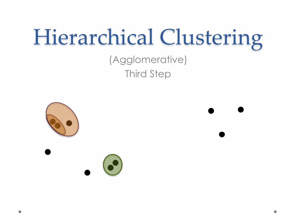
Hierarchical Clustering(Agglomerative)

Third Step

Hierarchical Clustering(Agglomerative)

Forth Step

Hierarchical Clustering(Agglomerative)

Fifth Step

Hierarchical Clustering(Agglomerative)

Sixth Step

Hierarchical Clustering(Agglomerative)

Seventh Step

We might have known that we only wanted 3 clusters, in which case we’d stop once we had 3.

Hierarchical Clustering(Agglomerative)

Eighth Step

Hierarchical Clustering(Agglomerative)

Final Step

Hierarchical Clustering

1

2

3

4

65

7

8

9

Levels of the Dendrogram

Resulting Dendrogram

A B C D E F G H I J

9

8

7

6

5

4

3

2

1

LinkagesWhich clusters/points are closest to each other?

How do I measure the distance between a point/cluster and a

cluster?

Linkages

Single Linkage: Distance between the closest points in the clusters.(Minimum Spanning Tree)

Linkages

Complete Linkage: Distance between the farthest points in the clusters.

Linkages

Centroid Linkage: Distance between the centroids (means) of each cluster. x

x

Linkages

Average Linkage: Averagedistance between all points in the clusters.

LinkagesWard’s Method: Increase in SSE (variance) when clusters are combined.

Ø Default in SAS PROC CLUSTERØ Shown mathematically similar to

centroid linkage

x

centroid for cluster i, ci

data points in cluster i:x1 , x2 , … , xNi

Hierarchical ClusteringSummary

Ø DisadvantagesØ Lacks global objective function: only makes decision based on local

criteria. Ø Merging decisions are final. Once a point is assigned to a cluster, it stays

there. Ø Computationally intensive, large storage requirements, not good for large

datasetsØ Poor performance on noisy or high-dimensional data like text.

Ø AdvantagesØ Lacks global objective function: no complicated algorithm or problem

with local minimaØ Creates hierarchy that can help choose the number of clusters and

examine how those clusters relate to each other.Ø Can be used in conjunction with other faster methods

k-Means Clustering(PROC FASTCLUS in SAS)

Ø The most popular clustering algorithm

Ø Tries to minimize the sum of squared distances from each point to its cluster centroid. (Global objective function)

x

x

Cluster 1 (C1) centroid c1

Cluster 2 (C2) centroid c2

data points in Cluster 2

data points in Cluster 1

k-Means AlgorithmØ Start with k “seed points”

Ø Randomly initialized (most software)Ø Determined ‘methodically’ (SAS PROC FASTCLUS)

Ø Assign each data point to the closest seed point. Ø The seed point then represents a cluster of dataØ Reset seed points to be the centroids of the clusterØ Repeat steps 2-4 updating the cluster centroids until

they do not change.

k-Means Interactive Demo

http://home.deib.polimi.it/matteucc/Clustering/tutorial_html/AppletKM.html

(You may have to add the site to your exceptions list on the Java Control Panel to view.)

Ø Most distances like Euclidean, Manhattan, or Max will provide similar answers.

Ø Use cosine distance (really 1-cos since cosine measures similarity) for text data. This is called spherical k-means.

Ø Using Mahalanobis distance is essentially the Expectation-Maximization (EM method) for Gaussian Mixtures.

Choice of Distance Metric

Determining Number of Clusters (SSE)

Ø Try the algorithm with k=1,2,3,…Ø Examine the objective function valuesØ Look for a place where the marginal benefit to

objective function for adding a cluster becomes small

k=1 objective function (SSE) is 902

Determining Number of Clusters (SSE)

Ø Try the algorithm with k=1,2,3,…Ø Examine the objective function valuesØ Look for a place where the marginal benefit to

objective function for adding a cluster becomes small

k=2 objective function (SSE) is 213

Determining Number of Clusters (SSE)

Ø Try the algorithm with k=1,2,3,…Ø Examine the objective function valuesØ Look for a place where the marginal benefit to

objective function for adding a cluster becomes small

k=3 objective function (SSE) is 193

Determining Number of Clusters (SSE)

Ø Try the algorithm with k=1,2,3,…Ø Examine the objective function valuesØ Look for a place where the marginal benefit to

objective function for adding a cluster becomes small

0200400600800

1000

k=1 k=2 k=3 k=4

Objective Function “Elbow”

=> k=2

k-Means SummaryØ Disadvantages

Ø Dependent on initialization (initial seeds)Ø Can be sensitive to outliers

Ø If problem, should consider k-mediods (uses median not mean)Ø Have to input the number of clustersØ Difficulty detecting non-spheroidal (globular) clusters

Ø AdvantagesØ Modest time/storage requirements.Ø Shown you can terminate method after small number of iterations with

good results.Ø Good for wide variety of data types

Cluster Validation and Profiling

Additional Notes for Self-Study

Cluster ValidationHow do I know that my clusters are actually clusters?Ø Lots of techniques/metrics have been proposed

Ø Measure separation between clustersØ Measure cohesion within clusters

Ø All have merit, most are difficult to interpret in the context of statistical significance.

Cluster ValidationØ To establish statistical significance:

ØShow that you can’t do just as well with randomized data (i.e. assume the null hypothesis of no clusters)

ØSimulate ~1000 random data sets choosing from the distributions or ranges of your variables. Cluster them with the same number of clusters. Record the SSE (k-means objective function) or validity metric of choice. Use this to show that your actual SSE is far better than you could expect to achieve if no clusters exist.

Profiling ClustersNow that we have clusters, how do we describe them?

Ø Use basic descriptives and hypothesis tests to show differences between clusters

Ø Use a decision tree to predict clusterØ SAS EM has segment profiler node

Other types of Clustering(self-study)

Ø DBSCAN – Density based algorithm designed to find dense areas of points. Capable of identifying ‘noise’ points which do not belong to any clusters.

Ø Graph/Network Clustering – Spectral clustering and modularity maximization. Covered in Social Network Analysis in Spring.

Some Explanation of SAS’s Clustering Output

(SELF-STUDY)Because it’s not exceedingly easy to figure out online!

Cubic Clustering Criterion (CCC)Ø Only available in SAS (to my knowledge)Ø CCC > 2 means that clustering is goodØ 0 > CCC > 2 means clustering requires examinationØ If slightly negative, risk of outliers is lowØ If ~< -30 then risk of outliers is high

Ø Should not be used with single or complete linkage, but with centroid or ward’s method.

Ø Each cluster must have >10 observations.

Source: Tufféry, Stéphane. Data Mining and Statistics for Decision Making. Wiley 2011

Determining Number of Clusters with the Cubic Clustering Criterion (CCC)

Ø A partition into k clusters is good when we see a dip in CCC for k-1 clusters and a peak for k clusters.

Ø After k clusters, the CCC should either a gradually decrease or a gradual rise (the latter event happens when more isolated groups or points are present)1

Source: Tufféry, Stéphane. Data Mining and Statistics for Decision Making. Wiley 2011

Determining Number of Clusters with the Cubic Clustering Criterion (CCC)

Image Source: Tufféry, Stéphane. Data Mining and Statistics for Decision Making. Wiley 2011

Determining Number of Clusters with the Cubic Clustering Criterion (CCC)

WARNING: Do not expect the CCC to be common knowledge outside of the SAS domain.

‘Overall R-Squared’ and‘Pseudo-F’

These statistics draw connections between a final clustering and ANOVA.Ø Total Sum of Squares (SST) Ø Between Group Sum of Squares (SSB)Ø Within Group Sum of Squares (SSW)

Ø This is the k-means objective previously referred to as SSE.Ø Minimizing SSW => Maximizing SSB

Ø SST = SSB + SSW.Ø ‘Overall R2’ = SSB/SST

Ø b

Ø Goal: Automatic recognition of handwritten digitsØ Digit database of 250 samples from 44 writersØ Subjects wrote digits in random order inside boxes

of 500 by 500 tablet pixel resolutionØ Spatial resampling to obtain a constant number of

regularly spaced points on the trajectoryØ (𝑥#, 𝑥%) give the first point coordinateØ (𝑥', 𝑥() give the second point coordinate Ø etc.

Example: PenDigit Data

Example: PenDigit Data

proc fastclus data=datasets.pendigittestmaxclusters=10out = clus;

var x1--x16;run;

Example: PenDigit Data

The first step to creating your own hierarchical dendrogram.

Example: PenDigit Data

proc glm data= clus;class cluster;model x1 = cluster;run; quit;

Example: PenDigit Data

Example: PenDigit Data

Example: PenDigit Data

Essentially using the centroids as predictions and then computing R-

squared.