clustering methods professor: dr. mansouri presented by : muhammad abouei &mohsen ghahremani...
TRANSCRIPT

Clustering MethodsProfessor: Dr. Mansouri
Presented by : Muhammad Abouei &Mohsen Ghahremani Manesh

2
Clustering Methods
Density-Based Clustering Methods DBSCAN (Density Based Spatial Clustering of Applications with
Noise)
OPTICS (Ordering Points To Identify the Clustering Structure)
DENCLUE (DENsity-based CLUstEring)
Grid-based Clustering

3
Density Based Clustering

4
DBSCAN Concepts
ε -neighborhood: Points within ε distance (radius) of a point. MinPts: minimum number of points in cluster (ε-
neighborhood of that point).
ε-neighborhood of q
ε-neighborhood of p
MinPts = 5
where ε and MinPts are a user-defined function.

5
DBSCAN Concepts
Density : number of points within a specified radius (ε)
Density(p)=5

6
DBSCAN Concepts
Core point : A point is a core point if it has more than a specified number of points (MinPts) within ε These are points that are at the interior of a cluster
ε-neighborhood of q
ε-neighborhood of p
p is a core point (MinPts = 5)
q is not a core point.

7
DBSCAN Concepts
Directly density-reachable : point p is directly density-reachable from a point q w.r.t. ε , MinPts if
1. p belongs to ε -neighborhood of q,
2. q is a core point,
MinPts = 4
p is DDR from q.
q is not DDR from p!
DDR is an asymmetric relation.

8
DBSCAN Concepts
Density-reachable: A point p is density-reachable from a point q w.r.t. ε , MinPts if there is a chain of points P1, …, Pn , P1=q, Pn=p such that Pi +1is directly density-reachable from Pi .
Or, point p is density-reachable form q, if there is a path (chain of points) from p to q consisting of only core points.
MinPts = 4
p is DR from q.
q is not DR from p!
p is not core.
DR is an asymmetric relation.

9
DBSCAN Concepts
Density-connectivity: point p is density-connected to point q w.r.t. ε , MinPts if there is a point r such that both, p and q are density-reachable from r w.r.t. ε and MinPts.
MinPts = 4
p and q are density-connected.
DC is an symmetric relation.

10
DBSCAN Concepts
Border point : A border point has fewer than MinPts within ε, but is in the neighborhood of a core point
MinPts =5
ε = circle radius

11
DBSCAN Concepts
Noise (outlier) point : is any point that is not a core point nor a border point.
MinPts =5
ε = circle radius

12
DBSCAN Concepts
DBSCAN relies on a density-based notion of cluster. Cluster : a cluster C is a non-empty set of density-connected
points that is maximal w.r.t. density-reachability. Maximality: For all p, q; if q C and if ∈ p is density-reachable from
q w.r.t. ε and MinPts, then also p C.∈
MinPts = 3
ε = circle radius

13
DBSCAN Algorithm
Arbitrary select a point p Retrieve all points density-reachable from p w.r.t. ε and
MinPts. If p is a core point, a cluster is formed. If p is a border point, no points are density-reachable from p
and DBSCAN visits the next point of the database. Continue the process until all of the points have been
processed.

14
DBSCAN
MinPts = 4

15
DBSCAN
DBSCAN is Sensitive to Parameters. MinPts = 4

16
DBSCAN
Core, Border and Noise Points: MinPts = 4, ε = 10
Original Points Point types: core, border
and noise

17
DBSCAN
When DBSCAN works well: Resistant to Noise Can handle clusters of different shapes and sizes
Original Points Clusters

18
DBSCAN
When DBSCAN does not work well: Varying densities High-dimensional data

19
DBSCAN Complexity
If a spatial index (ex, kd-tree, R*-tree) is used, the computational complexity of DBSCAN is O(n.logn), where n is the number of database objects. Otherwise, it is O(n2).

20
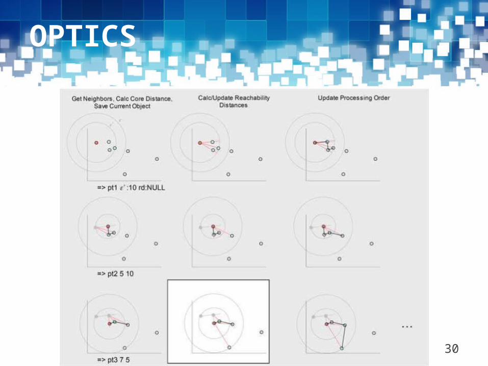
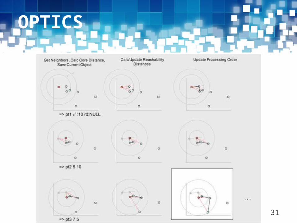
OPTICS
Core distance: smallest ε that makes it a core object. If p is
not core, it is undefined.
Core Distance of p or ε′ : distance between p and its 4-thNN.
MinPts = 5
ε = 3 cm

21
OPTICS
Reachability distance: of r w.r.t. p is the greater value of the core distance
of p and the Euclidean distance between p & r. If p is not a core object,
distance reachability between p & q is undefined.
reachability-distance ε, MinPts(p, r) = ε′
reachability-distance ε, MinPts(p, r′) = d(p, r′ )
MinPts = 5
ε = 3 cm

22
OPTICS

23
OPTICS

24
OPTICS

25
OPTICS

26
OPTICS

27
OPTICS

28
OPTICS

29
OPTICS
30
OPTICS
31
OPTICS

32
OPTICS
Color image segmentation using density-Based clustering

33
DENCLUE
DENCLUE (DENsity-based CLUstEring)
Major features
Solid mathematical foundation
Good for data sets with large amounts of noise
Allows a compact mathematical description of arbitrarily shaped clusters in
high-dimensional data sets
Significant faster than existing algorithm (faster than DBSCAN by a factor of
up to 45)
But needs a large number of parameters
34
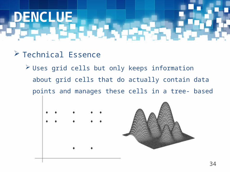
DENCLUE
Technical Essence
Uses grid cells but only keeps information about grid cells that do
actually contain data points and manages these cells in a tree- based
access structure.

35
DENCLUE
Technical Essence
DENCLUE is based on the following concepts:
Influence function
Density function
Density attractors.

36
DENCLUE
Influence function : The influence function f y(x) for a point
(data space) at point x is a positive function that decays to zero
as x “moves away” from .
Typical examples are:
and
where σ is a user-defined function.

37
DENCLUE
Density function :The density function at x based on a data space of
N points; i.e. D = {x1,…, xN}; is defined as the sum of the influence
function of all data points at x :
The goal of the definition: Identify all “significant” local maxima, xj*, j=1,…,m of f D(x)
Create a cluster Cj for each xj* and assign to Cj all points of D that lie within
the “region of attraction” of xj*.

38
DENCLUE
Example: Density Computation
D={x1,x2,x3,x4}
f DGaussian (x) = influence(x1)+influence(x2)+influence(x3)+influence(x4)
=0.04+0.06+0.08+0.6=0.78
Remark: the density value of y would be larger than the one for x.

39
DENCLUE
Density attractors :Density attractors are local maxima of the
overall density function f D(x). Clusters can then be determined mathematically by identifying density
attractors. A hill-climbing algorithm guided by the gradient can be used to determine
the density attractor of a set of data points.

40
DENCLUE
Density-attracted : A point x is density-attracted to a density
attractor x*, if there exists a set of points x0, x1, …, xk such
that x0 = x , xk = x* and the gradient of xi-1 is in the direction of
xi for 0<i<k.

41
DENCLUE
Center-Defined Cluster :A center-defined cluster (w.r.t. to σ, ε)
for a density attractor x* is a subset C D, with x C being
density-attracted by x* and f D(x) ε.
Outlier: Point x D is called outlier if it is density-attracted by
a local maximum xo* with f D(xo*) < ε.

42
DENCLUE
Multicenter defined clusters : Multicenter defined clusters are
a set of center-defined clusters linked by a path of
significance.

43
DENCLUE
An arbitrary-shape cluster : An arbitrary-shape cluster (w.r.t. to
σ, ) for a set of density attractors X is a subset C D, where
, x is density-attracted to , and
a path P from to with

44
DENCLUE
Note : that the number of clusters found by DENCLUE varies
depending on σ, .
45
DENCLUE
DENCLUE is able to detect arbitrarily shaped clusters.
The algorithm deals with noise very satisfactory.
The worst-case time complexity of DENCLUE is O(N.log2N).
Experimental results indicate that the average time complexity
is O(log2N).
It works efficiently with high-dimensional data.
DENCLUE needs at least 3 parameters to be determined, i.e.
σ, .

46
Grid-based
Using multi-resolution grid data structure Clustering complexity depends on the number of
populated grid cells and not on the number of objects in the dataset
Several interesting methods: CS Tree (Clustering Statistical Tree)STING WaveCluster

47
Grid-based
Basic Grid-based Algorithm 1. Define a set of grid-cells.
2. Assign objects to the appropriate grid cell and compute the density of each cell.
3. Eliminate cells, whose density is below a certain threshold τ.
4. Form clusters from contiguous (adjacent) groups of dense cells (usually minimizing a given objective function).

48
Grid-based
Fast: No distance computations,Clustering is performed on summaries and not individual
objects; complexity is usually O(no_of_populated_grid_cells) and not O(no_of_objects),
Easy to determine which clusters are neighboring.

49
References
A. K. Jain and R. C. Dubes. Algorithms for Clustering Data. Prentice Hall, 1988. A.K. Jain and M. N. Murty and P.J. Flynn, Data Clustering: A Review, ACM
Computing Surveys, vol 31. No 3,pp 264-323, 1999. A. L. N. Fred, J. M. N. Leitão, A New Cluster Isolation Criterion Based on
Dissimilarity Increments, IEEE “Optimal grid-clustering: Toward breaking the curse of dimensionality in high-
dimensional clustering,”in Proc. 25th VLDB Conf.,1999, pp. 506–517.

50
?