1

CO2QUEST

Optimal Valve Spacing for Next

Generation CO2 Pipelines

Dr Solomon BrownH. Mahgerefteh, V. Sundara & S. Martynov

University College London

http://www.co2quest.eu

2CO2QUEST

By 2050 200,000-360,000 km of pipeline will be

required for transportation of CO2 captured from

fossil fuel power plant for subsequent

sequestration (IEA, 2009).

Introduction

33

CO2 pipeline transportation – hazards

At concentrations higher than 10%, CO2 gas is toxic and can even be

fatal.

In the event of the accidental leakage/ release of CO2 from a pipeline:

• the CO2 gas can accumulate to potentially dangerous concentrations

in low-lying areas,

• the released cloud could cover an area of several square kilometres.

Courtesy of Laurence Cusco, HSL

4

CO2 pipeline transportation – hazards cont.

5

Individual risk contours (10

cpm/year, 1 cpm/year and 0.3

cpm/year) using TWODEE-2 dose

results

Geographical distribution of the

Potential loss-of-life (PLL) or EV

density map

6

Risk transects at regularly spaced points

along the pipeline route

0.1 cpm/year

1 cpm/year

10 cpm/year

7

• A rigorous mathematical model for dynamic valve closure

during pipeline decompression is developed

• Methodology is developed for a hazard-based optimisation of

valve spacing

• Optimal valve spacing for a realistic Case Study is found to be

ca. 15 km

• This is remarkably similar to current industrial standards for

gas pipelines in the UK

Presentation headlines

8

COOLTRANS Experimental release tests

Smaller scale venting tests,

primarily of interest for

maintenance

Large scale release tests and

fracture

9

Pressurised CO2

Rupture

plane: 1 atm

• At the rupture plane the fluid is exposed to ambient air

• Following the rupture, the rarefaction wave starts propagating along the

pipe

• The vapour phase emerges in the expansion wave

Physics of decompression

10

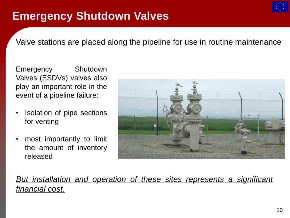
Emergency Shutdown

Valves (ESDVs) valves also

play an important role in the

event of a pipeline failure:

• Isolation of pipe sections

for venting

• most importantly to limit

the amount of inventory

released

Valve stations are placed along the pipeline for use in routine maintenance

Emergency Shutdown Valves

But installation and operation of these sites represents a significant

financial cost.

11

908 mm

P2, T2 transducers

135 m

Reservoir pipe

Closed end51 m

49 m

Rupture plane

P1, T1 transducers

113 m

Release pipe

146 mm

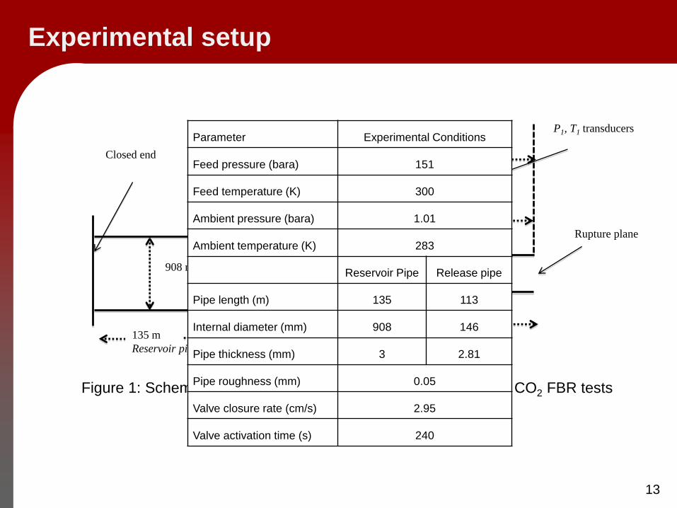
Figure 1: Schematic of the experimental set-up employed for the CO2 FBR tests

Experimental setup

12

Governing Equations:

Where ρ, u, P and h are the density, velocity, pressure and specific

enthalpy of the homogeneous fluid as function of time, t, and space, x.

qh is the heat transferred through the pipe wall to the fluid.

Release behaviour- rigorous outflow model

More advanced models:

Brown et al. (2013) Int. J. Greenh. Gas Control

Brown et al. (2014) Int. J. Greenh. Gas Control

13

908 mm

P2, T2 transducers

135 m

Reservoir pipe

Closed end51 m

49 m

Rupture plane

P1, T1 transducers

113 m

Release pipe

146 mm

Figure 1: Schematic of the experimental set-up employed for the CO2 FBR tests

Parameter Experimental Conditions

Feed pressure (bara) 151

Feed temperature (K) 300

Ambient pressure (bara) 1.01

Ambient temperature (K) 283

Reservoir Pipe Release pipe

Pipe length (m) 135 113

Internal diameter (mm) 908 146

Pipe thickness (mm) 3 2.81

Pipe roughness (mm) 0.05

Valve closure rate (cm/s) 2.95

Valve activation time (s) 240

Experimental setup

14

0

20

40

60

80

100

120

140

160

180

0 100 200 300 400

Pre

ssu

re (

bara

)

Time (s)

P₁ experimental

P₁ simulation

Valve closure

Valve activation

0

20

40

60

80

100

120

140

160

180

0 100 200 300 400

Pre

ss

ure

(b

ara

)

Time (s)

P₂ experimental

P₂ simulation

Valve closure

Valve activation

Comparison with predictions: Pressure

180

200

220

240

260

280

300

320

0 100 200 300 400

Tem

pera

ture

(K

)

Time (s)

T₁ experimental

T₁ simulation

Valve closure

Valve activation

Triple point

15

250

260

270

280

290

300

310

0 100 200 300 400

Tem

pera

ture

(K

)

Time (s)

T₂ experimental

T₂ simulation

Valve closure

Valve activation

Comparison with predictions: Temperature

Can we calculate the optimal number of valves

for a given pipeline to simultaneously reduce

costs and hazard posed by potential failure?

16

17

The problem is posed as a simple trade-off between the reduction in

the consequences of failure offered by the valve and the cost:

VPN is the single valve cost (€)

r is the average life time of the equipment (y)

n is the discount rate

L is the overall length of the pipeline (km)

D is the distance between consecutive valves (km)

The total valve cost for installation, J2 , is calculated using (Medina et

al., 2012):

Problem definition

18

The definition of J1 problematic because must:

1. Incorporate the effect emergency shutdown on the release

behaviour

2. Simulate the dispersion of the released CO2 cloud

• A detailed model for the dispersion is not practical for

optimisation (typically this can require months of HPC

resources)

• Dense gas dispersion model SLAB utilised

3. Define a meaningful metric for the hazard from the above

Problem definition cont.

19

Figure 2: Variation of concentration contours for 4 sampling sets

Disperion of cloud - SLAB

20

From the cloud dispersion model could calculate Dangerous Toxic

Loads given a population density with either the:

• SLOD (Significant Likelihood of Death)

• SLOT (Specified Level of Toxicity)

But for CO2 these are contentious so we select a simple measure:

• Quasi-steady CO2 concentration of contours calculated at

given intervals

• Time averaged area bounded by the 7 % contour was

calculated and used for J1

Definition: J1

21

Find the optimal valve spacing for a typical 96 km pipeline with a

Full Bore Rupture at 48 km

Optimisation Case Study

A parallel Monte Carlo simulation using 30 different randomly

generated valve spacings was performed to generate the Pareto

set.

Emergency valves placed upstream and

downstream of failure

22

Parameter Value Parameter Value

Pipeline Boundary Conditions

Pipeline external

diameter610 mm Upstream end Constant pressure

Pipeline wall

thickness19.4 mm Downstream No back flow

Pipeline wall

roughness0.005 mm Initial Conditions

Pipeline length 96 km Pressure in pipe 151 bara

Pipeline angle Horizontal Temperature in pipe 30 °C

Ambient temperature 10 °C

Table 1. Pipeline characteristics and fluid conditions for failure scenario.

Optimisation Case Study cont.

23

0

5

10

15

20

25

30

35

0 50 100 150 200

Cro

ssw

ind

Dis

tan

ce (

m)

Downwind Distance (m)

180 s

1260 s

2340 s

2880 s

3060 s

Figure 3: Variation of 7 % concentration half-contours with time

7 % concentration contours

24

0

0.1

0.2

0.3

0.4

0.5

0.6

0.7

0.8

0.9

1

0 10 20 30 40

No

rmal

ise

d V

alu

e

Valve Spacing (km)

Normalised Valve Cost (J₁)

Normalised Area Spanned (J₂)

Figure 4: Normalised valve cost and area spanned by 7 %

concentration

Objective curves

25

0

0.1

0.2

0.3

0.4

0.5

0.6

0.7

0.8

0.9

1

0 0.2 0.4 0.6 0.8 1

No

rmal

ise

d A

rea

Span

ne

d b

y th

e

7%

(vo

l./v

ol.

) C

on

cen

trat

ion

C

on

tou

r (J

1)

Normalised Valve Cost (J2)

Figure 5: Normalised Pareto set

Pareto set

26

0

0.2

0.4

0.6

0.8

1

1.2

1.4

0 10 20 30 40

1-N

orm

Valve Spacing (km)

Figure 6: Results under 1-Norm

0

0.2

0.4

0.6

0.8

1

1.2

0 10 20 30 40

∞-N

orm

Valve Spacing (km)

Figure 7: Results under ∞-Norm

Comparison of trade-off curves

27

• A rigorous mathematical model for dynamic valve closure

during pipeline decompression is developed

• Methodology is developed for a hazard-based optimisation of

valve spacing

• Optimal valve spacing for a realistic Case Study is found to be

ca. 15 km

• This is remarkably similar to current industrial standards for

gas pipelines in the UK

Conclusions

28

Acknowledgements and Disclaimer

The research leading to the results described in this

presentation has received funding from the European

Union 7th Framework Programme FP7-ENERGY-2012-1-

2STAGE under grant agreement number 309102.

The presentation reflects only the authors’ views and the

European Union is not liable for any use that may be

made of the information contained therein.

CO2QUEST

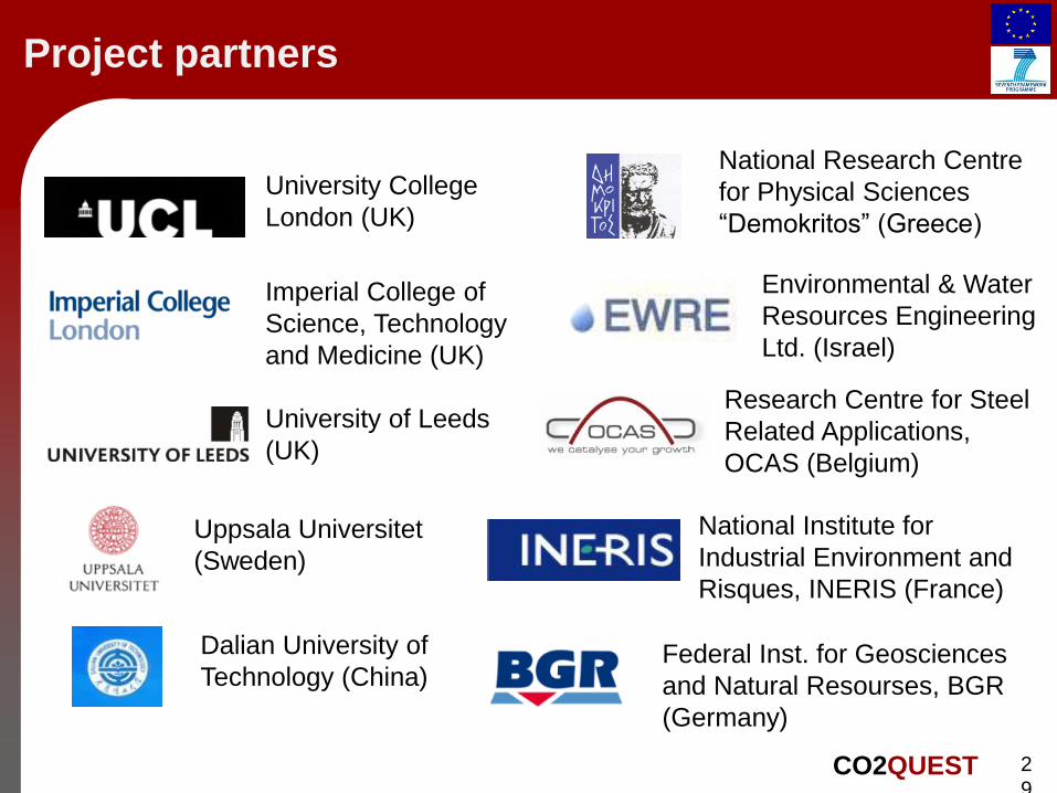
Project partners

2

9CO2QUEST

National Research Centre

for Physical Sciences

“Demokritos” (Greece)

Research Centre for Steel

Related Applications,

OCAS (Belgium)

Imperial College of

Science, Technology

and Medicine (UK)

University College

London (UK)

University of Leeds

(UK)

National Institute for

Industrial Environment and

Risques, INERIS (France)

Uppsala Universitet

(Sweden)

Federal Inst. for Geosciences

and Natural Resourses, BGR

(Germany)

Environmental & Water

Resources Engineering

Ltd. (Israel)

Dalian University of

Technology (China)

30CO2QUEST

Contact details

Solomon Brown

University College London

Gower Street, London,

United Kingdom

Tel: +44-2076793809

www.co2quest.eu

Thank you

Questions