coalgebraic foundations of linear systems

Coalgebraic Foundations of Linear Systems(An Exercise in Stream Calculus)

J.J.M.M. Rutten

CWI and Vrije Universiteit Amsterdam

Abstract. Viewing discrete-time causal linear systems as (Mealy) coal-gebras, we describe their semantics, minimization and realisation as uni-versal constructions, based on the final coalgebras of streams and causalstream functions.

1 Introduction

Linear systems are a fundamental mathematical structure with applications incontrol theory, signal processing, and telecommunications. In computer science,they are given but little attention. However, linear systems provide a mathe-matical model for various types of networks, including signal flow graphs andlinear sequential Boolean circuits (see, for instance, [Koh78, Lah98]). Such net-works are highly relevant for the foundations of computing, being elementaryand beautiful examples of the combined occurrence of memory and feedback.

In this paper, we give a coalgebraic account of the semantics of the followingelementary type of linear system: a (state-based) discrete-time (strongly) causallinear system consists of a vector space V of states; vector spaces I and Oof inputs and outputs; and linear maps F : V → V , describing the system’sdynamics, and G : I → V and H : V → O, describing the system’s input andoutput. We shall model such a system as a Mealy automaton (V, Φ), defined by

Φ : V → (O × V )I Φ(v)(i) = 〈H(v), F (v) + G(i)〉

Such Mealy automata, or (I, O)-systems as we shall call them here, are coal-gebras of the functor F : Set → Set defined by F(S) = (O × S)I . The choiceto model linear systems as Mealy automata or, in other words, as coalgebrasof this particular choice of functor F , is motivated by the following observa-tion: In [Rut06], it is shown that the final coalgebra of F , which is to serve asour semantic universe, is (isomorphic to) the set Γ of all causal functions fromthe set of input streams Iω to the set of output streams Oω . In system theory,the input-output behavior of a linear discrete-time causal system is often de-scribed in terms of precisely such a causal stream function (traditionally calledthe transfer function of the system).

Note that we work in the category of sets and functions rather than vectorspaces and linear maps. Although the functor F can also be defined on vectorspaces, the function Φ defined above will in general not be linear, even if F ,G, and H are. However, linearity of these maps does play a role in the various

T. Mossakowski et al. (Eds.): CALCO 2007, LNCS 4624, pp. 425–446, 2007.c© Springer-Verlag Berlin Heidelberg 2007

426 J.J.M.M. Rutten

characterisations of the semantics of linear systems, as we shall see later. (And,of course, vector addition in V is used in the definition of Φ.)

Once the functor (that is, the type of our systems) has been fixed and itsfinal coalgebra identified, a coalgebraic treatment of linear systems follows fromgeneral insights of universal coalgebra: the behaviour (or semantics) of a systemis given by the unique homomorphism into the final coalgebra; the image ofthis homomorphism constitutes the system’s minimisation; and systems can bespecified by elements of the final coalgebra and then realised (synthesised) bythe corresponding generated subsystems of the final coalgebra.

The exercise mentioned in the title then consists of working out the details ofall this. We view the formulation and the carrying out of this exercise as the maincontribution of the present paper. Technically, we had to extend our earlier work[Rut03, Rut05] a bit in order to deal with streams of linear transformations, inSection 3. After recalling the coalgebraic treatment of (I, O)-systems, in Section4, the main technical contribution lies in Section 5. It will be based on theelementary but crucial observation that the function Φ above factors throughthree maps of the following type (see (21)):

Φ : V �� V × V �� O × V �� (O × V )I

This is the basis for Theorem 8, which presents the final behaviour of (V, Φ) as thecomposition of three corresponding final homomorphisms. This final semanticsf assigns to each (initial) state v ∈ V a causal function f(v) : Iω → Oω (calledthe transfer function in system theory). This leads then to characterisationsof system minimization and realisation, in Sections 6 and 7. Surprisingly, thefinal semantics f turns out to be the composition of a (linear) final mappingH × F : V → Oω followed by a (non-linear) injection g : Oω → Γ . As aconsequence, minimization and realisation can be simply described in terms ofjust output streams, ignoring the presence of input streams altogether.

From the perspective of the theory of coalgebra, the relevance of our contri-bution consists of the following points. (i) It adds one more basic but importantexample to the family of mathematical structures that can be treated naturallyand fairly completely by coalgebraic means. Other well-known examples arestreams, automata, formal power series, infinite data types etc. (ii) Technically,the interaction between algebra and coalgebra is interesting. In general, (I, O)-systems (Mealy automata) live in the category of sets. As we shall see, linear(I, O)-systems are completely determined by their underlying linear O-systems(in which input plays no role), and these do live in the category of vector spacesand linear maps. As a consequence, the final behaviour of linear (I, O)-systems,which itself is obtained in Set, can be pleasantly characterised in terms of thebasic operations (of sum and convolution product) of stream calculus. (iii) Italso follows that streams – which constitute the prototypical example of a finalcoalgebra – are essentially all that is needed for the modelling of linear systems,since O-systems can be completely described in terms of O-streams. (iv) Thefinal behaviour of finite dimensional linear (I, O)-systems will be characterisedin terms of rational streams, in essentially the same way as finite deterministic

Coalgebraic Foundations of Linear Systems 427

automata, which can be viewed as elementary non-linear (I, O)-systems, cor-respond to rational (regular) languages. (v) More generally, the present modelshows that from a coalgebraic perspective, there is no essential difference be-tween the treatment of linear and non-linear systems. This opens the way forfuture applications of coalgebraic techniques to non-linear phenomena in systemtheory.

Some of these points may also be of interest for system theory, where thesemantics of the linear systems that we are considering is since long well under-stood (see, for instance, [Kai80]). In particular, our emphasis on the central roleof (the final coalgebra of) streams leads to a very elementary treatment of systemrealisation, which – depending on taste and background – might be consideredas a simpler alternative to Kalman’s [Kal63, KFA69] classical construction usingHankel matrices. See the appendix for a further discussion of this.

We mention a few directions for further research. Since the semantics of bothlinear and non-linear systems is given by finality, it would be interesting to tryand fit instances of non-linear systems from system theory (cf. [Son79]) into thecoalgebraic framework. Also generalisations to continuous systems could be con-sidered. Finally, one of the hallmarks of coalgebra is the notion of bisimulation,or observational equivalence, which comes along with every (functor) type ofsystem. It should therefore be possible to study notions of equivalence for linearsystems, including recently introduced ones such as in [Pap03] and [vdS04], froma coalgebraic perspective.

2 Preliminaries

We define the set of streams over a given set A by

Aω = {σ | σ : {0, 1, 2, . . .} → A}

We will denote elements σ ∈ Aω by σ = (σ(0), σ(1), σ(2), . . .). We define thestream derivative of a stream σ by

σ′ = (σ(1), σ(2), σ(3), . . .)

and we call σ(0) the initial value of σ. For a ∈ A and σ ∈ Aω we use the followingnotation:

a : σ = (a, σ(0), σ(1), σ(2), . . .)

For instance, σ = σ(0) : σ′, for any σ ∈ Aω. Any function f : A → B induces afunction

fω : Aω → Bω fω(σ) = (f(σ(0)), f(σ(1)), f(σ(2)), . . .) (1)

Any function f : A → A induces a function

f : A → Aω f(a) = (a, f(a), f2(a), . . .) (2)

428 J.J.M.M. Rutten

where f0 = 1, the identity on A and fn+1 = f ◦ fn. If V is a set and W is avector space (over some field k) then the set WV of all functions

WV = {f | f : V → W}

is a vector space, with addition and scalar multiplication given, for v ∈ V andc ∈ k, by

(f + g)(v) = f(v) + g(v) (c · f)(v) = c · f(v)

In particular, if V is a vector space over k then so is the set V ω of all streams overV . Both the operations of initial value and derivative are linear transformations:for all c, d ∈ k, σ, τ ∈ V ω,

(c · σ + d · τ)(0) = c · σ(0) + d · τ(0) (c · σ + d · τ)′ = c · σ′ + d · τ ′

For any set A and n ≥ 1, we denote the elements v ∈ An by v = (v1, . . . , vn). Itwill sometimes be convenient to switch between streams of tuples and tuples ofstreams. We define the transpose as follows:

(−)T : (An)ω → (Aω)n (σT )i(j) = (σ(j))i (3)

This function is an isomorphism and has an inverse which we denote again by

(−)T : (Aω)n → (An)ω

A semi-ring is a set R with a commutative operation of addition c + d; a(generally non-commutative) operation of multiplication c · d with c · (d + e) =(c · d) + (c · e) and (d + e) · c = (d · c) + (e · c); and with neutral elements 0 and 1such that c + 0 = c, 1 · c = c · 1 = c and c · 0 = 0 · c = 0. If every c ∈ R moreoverhas an additive inverse −c (with c + (−c) = 0) then R is a ring.

Any field is a ring. The following example of a ring will be used later. Let Vbe a vector space (over some field k). The set V →L V of linear maps F : V → Vis a ring with addition and multiplication defined by

(F + G)(v) = F (v) + G(v) (F × G)(v) = F (G(v))

and with the everywhere zero map and the identity map as neutral elements 0and 1.

3 Stream Calculus

Let R be a ring. We define the following operators on the set Rω of streams overR, for all c ∈ R, σ, τ ∈ Rω, n ≥ 0:

[c] = (c, 0, 0, 0, . . .) (often simply denoted again by c)X = (0, 1, 0, 0, 0, . . .)

(σ + τ)(n) = σ(n) + τ(n) [sum]

(σ × τ)(n) =n∑

i=0

σ(i) · τ(n − i) [convolution product]


(where · denotes multiplication in the ring R). A stream σ has a (unique)multiplicative inverse σ−1 in Rω:

σ−1 × σ = [1]

whenever its initial value σ(0) has a multiplicative inverse σ(0)−1 in R. Asusual, we shall often write 1/σ for σ−1 and σ/τ for σ × τ−1. Since X2 =(0, 0, 1, 0, 0, 0, . . .), X3 = (0, 0, 0, 1, 0, 0, 0, . . .) and so on, the following infinitesum is well defined, for all σ ∈ Rω:

σ = σ(0) + (σ(1) × X) + (σ(2) × X2) + · · ·

(Note that we write σ(i) for [σ(i)]; similarly below.) It shows that σ can beviewed as a formal power series in the indeterminate X (which here in fact is aconstant stream). What distinguishes our approach from formal power series is asystematic use of the operation of stream derivative and the universal propertyof finality it induces (see Section 4). This leads to a somewhat non-standardalgebraic calculus, which we call stream calculus. We mention a few identitieswhich are helpful for the computation of stream derivatives. (Computing streamderivatives is crucial in our approach to system realisation, in Section 7).

Lemma 1 ([Rut03]). Let R be a ring. For all σ, τ ∈ Rω,

(σ + τ)′ = σ′ + τ ′

(σ × τ)′ = (σ′ × τ) + (σ(0) × τ ′)(σ−1)′ = −σ(0)−1 × σ′ × σ−1

and (σ + τ)(0) = σ(0) + τ(0), (σ × τ)(0) = σ(0) · τ(0), and σ−1(0) = σ(0)−1 (ifthe latter exists). Moreover, σ = σ(0) + (X × σ′) and X × σ = σ × X . �

We call a stream polynomial if it is of the form

c0 + (c1 × X) + (c2 × X2) + · · · + (ck × Xk)

A stream is rational if it is the quotient σ/τ = σ × τ−1 of two polynomial streamsσ and τ for which τ(0)−1 exists. We denote the set of all rational streams over R by

Rat(Rω) = {σ ∈ Rω | σ is rational}

A prototypical example of a rational stream in Rω, for c ∈ R, is

11 − (c × X)

= (1, c, c2, . . .)

If we consider the ring V →L V , for a vector space V , then streams φ ∈ (V →L

V )ω are infinite sequences φ = (φ(0), φ(1), φ(2), . . .) of linear transformationsφ(i) : V → V . For a linear transformation F ∈ (V →L V ), the example abovebecomes

11 − (F × X)

= (1, F, F 2, · · ·) (4)

430 J.J.M.M. Rutten

which, under the isomorphism (V → V )ω ∼= V → V ω, is equal to F defined in(2) above.

We shall also use the following type of convolution product. Let V and W bevector spaces. For streams φ ∈ (V →L W )ω and σ ∈ V ω, we define φ ×σ ∈ Wω by

(φ × σ)(n) =n∑

i=0

φ(i) × σ(n − i) (5)

where on the right we write φ(i) × σ(n − i) for φ(i)(σ(n − i)). For a linear mapH : V → W , we have as a special case

[H ] × σ = (H, 0, 0, 0, . . .) × σ = (H(σ(0)), H(σ(1)), H(σ(2)), . . .)

which equals Hω(σ) defined in (1) above. Note that if W = V , the set of streams(V →L V )ω has itself also an operation of convolution product, which interactsnicely with the product defined in (5). For example, for φ, ψ ∈ (V →L V )ω andσ ∈ V ω,

(φ × ψ) × σ = φ × (ψ × σ) (6)

Let k be a field. A linear transformation F : kn → km between finite dimen-sional vector spaces corresponds to an m × n matrix MF with values Fij in k:

F : kn → km MF =

⎛

⎜⎜⎜⎝

F11 F12 · · · F1n

F21 F22 · · · F2n

......

. . ....

Fm1 Fm2 · · · Fmn

⎞

⎟⎟⎟⎠

Here and in what follows, the matrix is with respect to the standard basis

(1, 0, . . . , 0), . . . , (0, . . . , 0, 1)

of kn and km. Any stream φ = (φ(0), φ(1), φ(2), . . .) of linear transformationsφ(i) : kn → km corresponds to a stream of matrices

(Mφ(0), Mφ(1), Mφ(2), . . .) = Mφ(0) + (Mφ(1) × X) + (Mφ(2) × X2) + · · ·

If we consider Mφ(i)×X i as an m×n matrix obtained from Mφ(i) by multiplyingeach of its entries by X i, then the infinite sum on the right can itself be viewedas an m × n matrix Mφ with entries in kω:

(Mφ)ij = (Mφ(0))ij + ((Mφ(1))ij × X) + ((Mφ(2))ij × X2) + · · · (7)

For the special case of [H ] = (H, 0, 0, 0, . . .), for a linear transformation H :kn → km, we have

(M[H])ij = ((MH)ij , 0, 0, 0, . . .) (8)

We will let the context determine whether entries in k or kω are intended, andwe shall simply write

M[H] = MH (9)


The correspondence between φ and Mφ is given by the following commutativediagram:

(kn)ωφ×(−)��

(−)T

��

(km)ω

(−)T

��(kω)n

Mφ×(−)�� (kω)m

(φ × σ)T = Mφ × σT (10)

(Recall the definition of (−)T from (3).) Here φ×(−) denotes convolution productand Mφ × (−) denotes matrix multiplication. Note that M1 = 1, where 1 on theleft denotes the stream (1, 0, 0, 0, . . .) (consisting of the identity map followed byzero maps), and 1 on the right denotes the identity matrix (having 1’s on thediagonal and 0’s everywhere else). Also note that

Mφ×ψ = Mφ × Mψ (11)

We have the following proposition.

Proposition 2. Let ρ ∈ (kn →L kn)ω be a stream of linear transformationsρ(i) : kn → kn. If ρ is rational then Mρ defined in (7) has entries in Rat(kω).

Proof: Consider two polynomial streams φ, ψ ∈ (kn →L kn)ω. The entries ofthe matrices Mφ and Mψ are polynomial streams in kω. If ψ moreover has aninverse ψ−1 then M1 = 1 and (11) imply Mψ−1 = (Mψ)−1, which has values inRat(kω). It follows that Mφ×ψ−1 = Mφ × (Mψ)−1 has values in Rat(kω). �

Example 3. Let k = IR and let F, G : IR2 → IR2 be linear transformationsdefined by

MF =(

1 10 0

)MG =

(0 −11 2

)

We compute the matrices of the rational streams F = ( 1 − (F × X) )−1 andG = ( 1 − (G × X) )−1:

MF = (M1−(F×X))−1 =(

1 − X −X0 1

)−1

=( 1

1−XX

1−X

0 1

)

MG = (M1−(G×X))−1 =(

1 X−X 1 − 2X

)−1

=1

(1 − X)2·(

1 − 2X −XX 1

)

�

4 Systems Coalgebraically

We recall the coalgebraic semantics of systems with input and output. States,inputs and outputs will be represented by plain sets, and homomorphisms will

432 J.J.M.M. Rutten

be simply functions between sets. In Section 5, we will look at the coalgebraicmodelling of linear systems, involving vector spaces and linear maps.

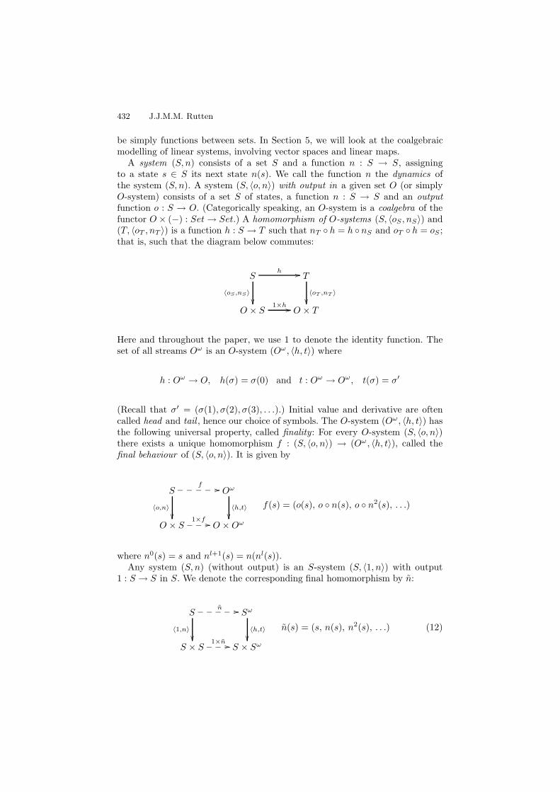
A system (S, n) consists of a set S and a function n : S → S, assigningto a state s ∈ S its next state n(s). We call the function n the dynamics ofthe system (S, n). A system (S, 〈o, n〉) with output in a given set O (or simplyO-system) consists of a set S of states, a function n : S → S and an outputfunction o : S → O. (Categorically speaking, an O-system is a coalgebra of thefunctor O × (−) : Set → Set.) A homomorphism of O-systems (S, 〈oS , nS〉) and(T, 〈oT , nT 〉) is a function h : S → T such that nT ◦ h = h ◦ nS and oT ◦ h = oS ;that is, such that the diagram below commutes:

Sh ��

〈oS,nS〉��

T

〈oT ,nT 〉��

O × S1×h �� O × T

Here and throughout the paper, we use 1 to denote the identity function. Theset of all streams Oω is an O-system (Oω , 〈h, t〉) where

h : Oω → O, h(σ) = σ(0) and t : Oω → Oω , t(σ) = σ′

(Recall that σ′ = (σ(1), σ(2), σ(3), . . .).) Initial value and derivative are oftencalled head and tail , hence our choice of symbols. The O-system (Oω , 〈h, t〉) hasthe following universal property, called finality: For every O-system (S, 〈o, n〉)there exists a unique homomorphism f : (S, 〈o, n〉) → (Oω , 〈h, t〉), called thefinal behaviour of (S, 〈o, n〉). It is given by

S

〈o,n〉��

f �� Oω

〈h,t〉��

O × S1×f �� O × Oω

f(s) = (o(s), o ◦ n(s), o ◦ n2(s), . . .)

where n0(s) = s and nl+1(s) = n(nl(s)).Any system (S, n) (without output) is an S-system (S, 〈1, n〉) with output

1 : S → S in S. We denote the corresponding final homomorphism by n:

S

〈1,n〉��

n �� Sω

〈h,t〉��

S × S1×n �� S × Sω

n(s) = (s, n(s), n2(s), . . .) (12)


We call n the fully observable behaviour of (S, n). The final behaviour f of anO-system (S, 〈o, n〉) factors through its fully observable behaviour n as follows:

S

〈1,n〉��

n��

〈o,n〉

��

f

��Sω

〈h,t〉��

oω�� Oω

〈h,t〉

��

S × S

o×1��

1×n�� S × Sω

o×1��

O × S1×n ��

1×f

��O × Sω 1×oω

�� O × Oω

f = oω ◦ n (13)

Next we consider systems with output and input. As before let O be a setof outputs. In addition, let I be an arbitrary set, the elements of which we callinputs . A system (S, φ) with input in I and output in O (or simply (I, O)-system)consists of a set S of states together with a function φ : S → (O × S)I . Thefunction φ maps a state s ∈ S to a function φ(s) : I → O × S that sends aninput i to a pair φ(s)(i) ∈ O×S. We shall sometimes use the following notation:

s1i|o �� s2 ⇐⇒ φ(s1)(i) = 〈o, s2〉

which can be read as: in state s1 and with input i the system changes to states2 while producing output o. Note that in general both the next state and theoutput depends on both the starting state and the input. Systems with input inI and output in O are also known in the literature as Mealy machines [Eil74].Categorically, an (I, O)-system is a coalgebra of the functor F : Set → Setdefined by F(S) = (O × S)I .

Let (S, φS) and (T, φT ) be two (I, O)-systems. For s1 ∈ S and i ∈ I letφ(s1)(i) = 〈o, s2〉. A homomorphism of (I, O)-systems is a function h : S → Tsuch that φT (h(s))(i) = 〈o, h(s2)〉, for all s1 ∈ S and i ∈ I. Equivalently, hshould make the diagram below commute:

Sh ��

φS

��

T

φT

��(O × S)I

(1×h)1 �� (O × T )I

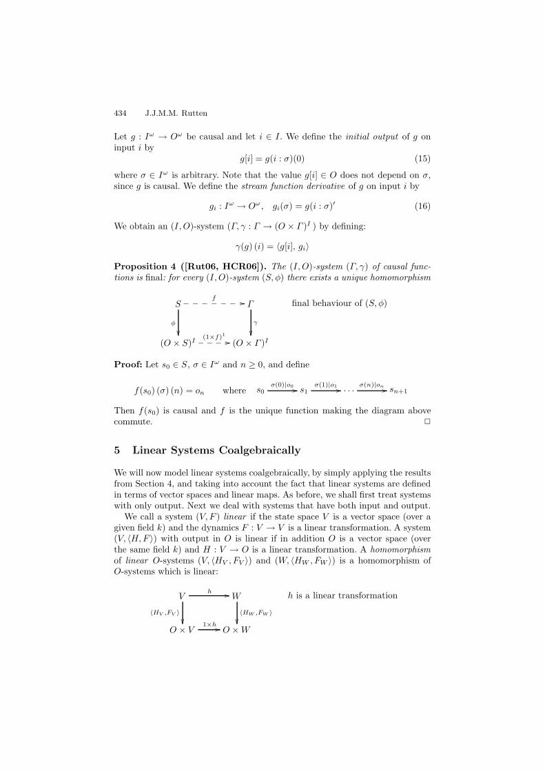
A final (I, O)-system can be constructed as follows. We call a function g : Iω →Oω causal (aka synchronous or letter-to-letter) if for any σ ∈ Iω the n-th elementof g(σ) depends on only the first n elements of the input σ; that is,

σ(0) = τ(0), . . . , σ(n) = τ(n) ⇒ g(σ)(n) = g(τ)(n)

for all σ, τ ∈ Iω and n ≥ 0. We denote the set of all causal functions by

Γ = { g : Iω → Oω | g is causal } (14)

434 J.J.M.M. Rutten

Let g : Iω → Oω be causal and let i ∈ I. We define the initial output of g oninput i by

g[i] = g(i : σ)(0) (15)

where σ ∈ Iω is arbitrary. Note that the value g[i] ∈ O does not depend on σ,since g is causal. We define the stream function derivative of g on input i by

gi : Iω → Oω , gi(σ) = g(i : σ)′ (16)

We obtain an (I, O)-system (Γ, γ : Γ → (O × Γ )I ) by defining:

γ(g) (i) = 〈g[i], gi〉

Proposition 4 ([Rut06, HCR06]). The (I, O)-system (Γ, γ) of causal func-tions is final: for every (I, O)-system (S, φ) there exists a unique homomorphism

Sf ��

φ

��

Γ

γ

��(O × S)I

(1×f)1 �� (O × Γ )I

final behaviour of (S, φ)

Proof: Let s0 ∈ S, σ ∈ Iω and n ≥ 0, and define

f(s0) (σ) (n) = on where s0σ(0)|o0 �� s1

σ(1)|o1 �� · · · σ(n)|on �� sn+1

Then f(s0) is causal and f is the unique function making the diagram abovecommute. �

5 Linear Systems Coalgebraically

We will now model linear systems coalgebraically, by simply applying the resultsfrom Section 4, and taking into account the fact that linear systems are definedin terms of vector spaces and linear maps. As before, we shall first treat systemswith only output. Next we deal with systems that have both input and output.

We call a system (V, F ) linear if the state space V is a vector space (over agiven field k) and the dynamics F : V → V is a linear transformation. A system(V, 〈H, F 〉) with output in O is linear if in addition O is a vector space (overthe same field k) and H : V → O is a linear transformation. A homomorphismof linear O-systems (V, 〈HV , FV 〉) and (W, 〈HW , FW 〉) is a homomorphism ofO-systems which is linear:

Vh ��

〈HV ,FV 〉��

W

〈HW ,FW 〉��

O × V1×h �� O × W

h is a linear transformation


Recall from Section 4 that the O-system (Oω , 〈h, t〉) is final among all (not nec-essarily linear) systems. We saw (in Section 2) that if O is a vector space thenOω is also a vector space. Since initial value and derivative are linear transfor-mations, (Oω , 〈h, t〉) is a linear O-system. The final behaviour f : V → Oω of anO-system (V, 〈H, F 〉) is given, according to (13), by

VF

��

f

��V ω

Hω�� Oω f(v) = Hω ◦ F (v)

This is equivalent, for all v ∈ V , to

f(v) = Hω ◦ F (v)= (H(v), H ◦ F (v), H ◦ F 2(v), . . .)= (H, 0, 0, 0, . . .) × (1, F, F 2, . . .) × (v, 0, 0, 0, . . .) [using (5) and (6)]= (H, 0, 0, 0, . . .) × F × (v, 0, 0, 0, . . .) [using (1, F, F 2, . . .) = F , as in (4)]= [H ] × F × [v]

Thus:

VF×[−]

��

f

��V ω

[H]×(−)�� Oω f(v) = [H ] × F × [v]

It follows that f is a linear transformation and that (Oω , 〈h, t〉) is final in thefamily of all linear O-systems and linear homomorphisms between them.

The final behaviour of finite dimensional linear O-systems can be furthercharacterised as follows. Let n, m ≥ 1 and consider a system (kn, 〈H, F 〉) withlinear transformations F : kn → kn and H : kn → km. By (10), the followingdiagram commutes:

(kn)ωF×(−) ��

(−)T

��

(kn)ω

(−)T

��

[H]×(−) �� (km)ω

(−)T

��(kω)n

MF ×(−)�� (kω)n

MH×(−)�� (kω)m

([H ]×F×(−))T = MH×MF ×(−)T

(17)(where we use the convention (9) of writing M[H] = MH). It follows that thefinal behaviour f satisfies

f(v)T = ([H ] × F × [v])T = MH × MF × [v]T (18)

We saw in (4) that F = (1 − (F × X))−1 is a rational stream. By Proposition 2,the matrix MF has values in Rat(kω). And so we have proved the following.

436 J.J.M.M. Rutten

Proposition 5. For a finite dimensional system (kn, 〈H, F 〉) with dynamics F :kn → kn and output H : kn → km, the final behaviour f : kn → km satisfies, forall v ∈ kn,

f(v)T = MH × MF × [v]T

and thus is obtained from [v]T by multiplication with an m×n matrix with valuesin Rat(kω). �

Example 6. Let k = IR and consider the linear system (IR2, 〈H, F 〉) with outputH : IR2 → IR and dynamics F : IR2 → IR2 given by

H =(1 1

)F =

(1 10 0

)

The matrix MF corresponding to F has been computed in Example 3:

MF =( 1

1−XX

1−X

0 1

)

The final behaviour f〈H,F 〉 : IR2 → IRω of this system is given, for any (a, b) ∈IR2, by

f〈H,F 〉(a, b) =(1 1

)×

( 11−X

X1−X

0 1

)×

(ab

)

=a + b

1 − X

(omitting square brackets around a and b as usual). Repeating the example witha different output function H and the same dynamics F :

H =(1 2

)F =

(1 10 0

)

leads to the following final behaviour:

f〈H,F 〉(a, b) =( 1

1−X2−X1−X

)×

(ab

)=

a + 2b − bX

1 − X

�

Next we discuss linear systems with input and output. We shall model them as(I, O)-systems, as defined in Section 4, and then study their final behaviour.

Let I, O and V be vector spaces over k, and let F : V → V , G : I → V andH : V → O be linear transformations. We define the (I, O)-system (V, Φ〈H,F,G〉)by

Φ〈H,F,G〉 : V → (O × V )I Φ〈H,F,G〉(v)(i) = 〈H(v), F (v) + G(i)〉 (19)

or equivalently, expressed in terms of transitions,

vi |H(v) �� F (v) + G(i)


We call (V, Φ〈H,F,G〉) a linear (I, O)-system because of the linearity of F , G,and H . However, note that Φ itself is not linear and likewise, homomorphismsof linear (I, O)-systems will generally not be linear. This is in contrast with thefamily of linear O-systems, where everything is linear.

For a linear(I, O)-system (V, Φ〈H,F,G〉) we call (V, 〈H, F 〉) its underlying O-system. The key to the coalgebraic understanding of a linear (I, O)-system is theobservation that its behaviour is in essence determined by that of its underlyingO-system.

The following lemma will be helpful. Consider the final O-system (Oω , 〈h, t〉)and an arbitrary linear transformation ψ : I → Oω . This gives rise to a linear(I, O)-system (Oω , Φ〈h,t,ψ〉), with Φ〈h,t,ψ〉 defined as in (19). The lemma belowdescribes its final behaviour g : Oω → Γ , introduced in Proposition 4.

Lemma 7. For all α ∈ Oω and σ ∈ Iω,

Oωg ��

Φ〈h,t,ψ〉

��

Γ

γ

��(O × Oω)I

(1×g)1�� (O × Γ )I

g(α)(σ) = α + (ψ × X × σ)

(On the right, we read ψ as a stream of linear transformations ψ ∈ (I →L O)ω ∼=I →L Oω.)

Proof: By finality of (Γ, γ), it is sufficient to show that the function g definedas above is a homomorphism of (I, O)-systems. By definition of γ, we haveγ(g(α))(i) = 〈 g(α)[i], g(α)i 〉, for all i ∈ I. Now

g(α)[i] = ( g(α)(i : σ) ) (0) = α(0)

and, for all σ ∈ Iω,

g(α)(i : σ) = g(α)(i + (X × σ)) [by Lemma 1, with i = (i, 0, 0, 0, . . .)]= α + (X × ψ × (i + (X × σ)) )= α + (X × ψ × i ) + (X × ψ × X × σ) (20)

This implies

g(α)i(σ) = ( g(α)(i : σ) )′ [definition stream function derivative (16)]= (α′ + (ψ × i) ) + (ψ × X × σ) [using (20) and Lemma 1]= g(α′ + ψ(i))(σ) [using ψ × i = ψ(i)]

It follows that

γ(g(α))(i) = 〈α(0), g(α′ + ψ(i)) 〉= (1 × g) ( 〈α(0), α′ + ψ(i) 〉 )=

((1 × g)1 ◦ Φ〈h,t,ψ〉 (α)

)(i) [definition Φ〈h,t,ψ〉 (19)]

438 J.J.M.M. Rutten

This shows that the diagram above commutes. Thus g is a homomorphism. �

Next we observe that for a linear (I, O)-system (V, Φ〈H,F,G〉), with Φ〈H,F,G〉 asin (19), the function Φ〈H,F,G〉 can be decomposed as follows:

V 〈1,F 〉��

Φ〈H,F,G〉

��V × V

H×1�� O × V

G+

�� (O × V )I (21)

where the function G+ is defined, for all o ∈ O, v ∈ V , and i ∈ I, by

G+(〈o, v〉)(i) = 〈o, v + G(i)〉

Theorem 8.The final behaviour1 f : V → Γ of a linear (I, O)-system (V, Φ〈H,F,G〉) (asdefined in (19)) satisfies, for all v ∈ V and σ ∈ Iω,

f(v)(σ) =(

[H ] × F × [v]T)

+(

[H ] × F × [G] × X × σ)

Proof: Let ψ : I → Oω be defined by ψ = [H ] × F × [G] and consider thefollowing diagram:

V

〈1,F 〉��

F

��

Φ〈H,F,G〉

f

��V ω

〈h,t〉��

Hω�� Oω

〈h,t〉

��

g�� Γ

γ

��

V × V

H×1��

1×F

�� V × V ω

H×1��

O × V1×F

��

G+��

(∗)

O × V ω

1×Hω�� O × Oω

ψ+��

(O × V )I

(1×(Hω◦F ))1��

(1×f)1

(O × Oω)I(1×g)1 �� (O × Γ )I

Recall that Hω = [H ] × (−), using the convolution product introduced in (5)and, consequently, Hω ◦ F = [H ]× F . The function ψ has been defined preciselysuch that the rectangle (∗) above commutes. (Note that a proof of (∗) will usethe linearity of [H ] × F .) The right hand pentagon commutes by Lemma 7.Everything else commutes by finality. �

The final behaviour of finite dimensional linear (I, O)-systems can be furthercharacterised, similarly to the case of linear O-systems. First we define for anycausal function g : (kl)ω → (km)ω a function.1 We observe that the final behaviour f(0) of the initial state 0 corresponds to what

is known in system theory as the transfer function of the system, where F is oftenexpressed as (zI − F )−1.


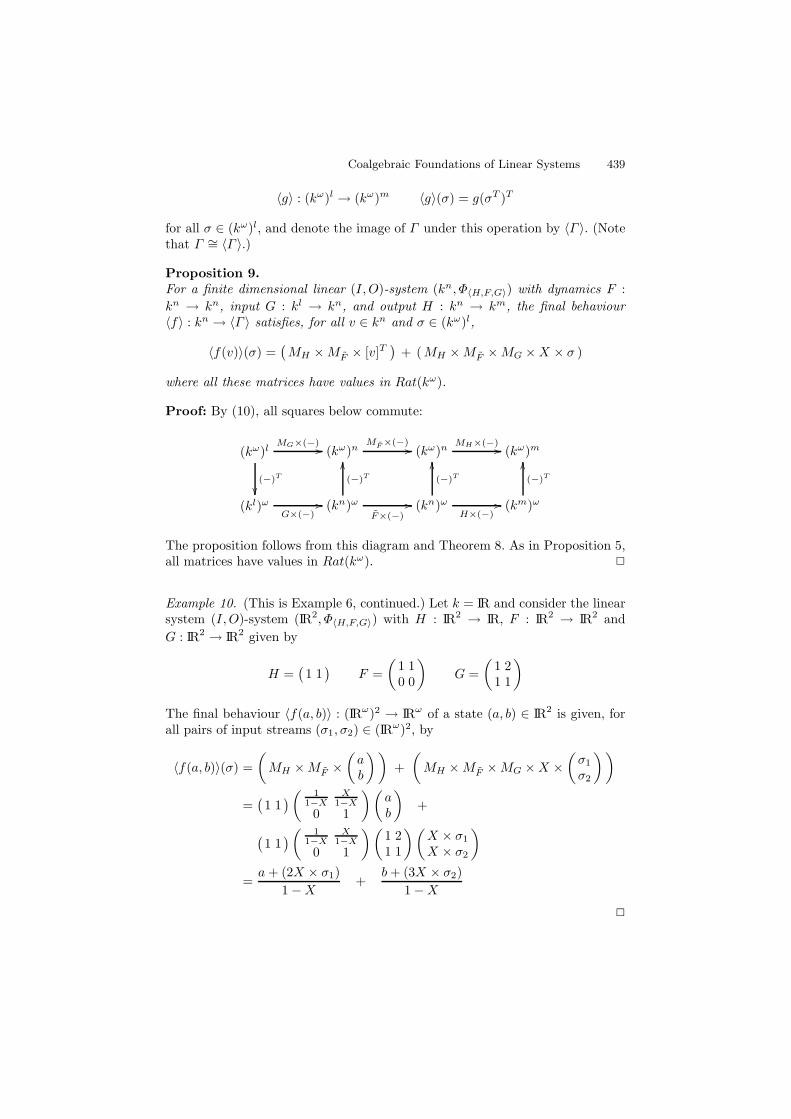
〈g〉 : (kω)l → (kω)m 〈g〉(σ) = g(σT )T

for all σ ∈ (kω)l, and denote the image of Γ under this operation by 〈Γ 〉. (Notethat Γ ∼= 〈Γ 〉.)

Proposition 9.For a finite dimensional linear (I, O)-system (kn, Φ〈H,F,G〉) with dynamics F :kn → kn, input G : kl → kn, and output H : kn → km, the final behaviour〈f〉 : kn → 〈Γ 〉 satisfies, for all v ∈ kn and σ ∈ (kω)l,

〈f(v)〉(σ) =(MH × MF × [v]T

)+ (MH × MF × MG × X × σ )

where all these matrices have values in Rat(kω).

Proof: By (10), all squares below commute:

(kω)l

(−)T

��

MG×(−) �� (kω)nMF ×(−) �� (kω)n

MH×(−) �� (kω)m

(kl)ω

G×(−)�� (kn)ω

F×(−)��

(−)T

��

(kn)ω

H×(−)��

(−)T

��

(km)ω

(−)T

��

The proposition follows from this diagram and Theorem 8. As in Proposition 5,all matrices have values in Rat(kω). �

Example 10. (This is Example 6, continued.) Let k = IR and consider the linearsystem (I, O)-system (IR2, Φ〈H,F,G〉) with H : IR2 → IR, F : IR2 → IR2 andG : IR2 → IR2 given by

H =(1 1

)F =

(1 10 0

)G =

(1 21 1

)

The final behaviour 〈f(a, b)〉 : (IRω)2 → IRω of a state (a, b) ∈ IR2 is given, forall pairs of input streams (σ1, σ2) ∈ (IRω)2, by

〈f(a, b)〉(σ) =(

MH × MF ×(

ab

) )+

(MH × MF × MG × X ×

(σ1σ2

) )

=(1 1

) ( 11−X

X1−X

0 1

) (ab

)+

(1 1

) ( 11−X

X1−X

0 1

) (1 21 1

) (X × σ1X × σ2

)

=a + (2X × σ1)

1 − X+

b + (3X × σ2)1 − X

�

440 J.J.M.M. Rutten

6 Minimization and Equivalence

Because O- and (I, O)-systems are coalgebras, the general definition of coalge-braic equivalence applies. Here we spell out these definitions together with theobservation that the corresponding minimization of a system is given by the (im-age under) the final behaviour mapping. For linear (I, O)-systems, we shall seethat minimization and equivalence are particularly simple, as they are entirelydetermined by their underlying O-systems.

Equivalence of (not necessarily linear) O-systems is defined as follows. A re-lation R ⊆ S × T is called an O-bisimulation between O-systems (S, 〈oS , nS〉)and (T, 〈oT , nT 〉) if for all s ∈ S and t ∈ T :

〈s, t〉 ∈ R ⇒{

oS(s) = oT (t) and〈nS(s), nT (t)〉 ∈ R

We say that s and t are O-equivalent and write s ∼O t if there exists an O-bisimulation R with 〈s, t〉 ∈ R. The final behaviour f : S → Oω of an O-system(S, 〈o, n〉) identifies precisely all O-equivalent states: s1 ∼O s2 iff f(s1) = f(s2),for all s1, s2 ∈ S. (For the elementary proof, see [Rut03].) As a consequence, theminimization of an O-system with respect to O-equivalence is given by the imageof S under f , which is a subsystem f(S) ⊆ Oω because f is a homomorphism.It follows that if the system is linear, then the greatest O-equivalence on S isgiven by the kernel ker(f).

For (I, O)-systems there exists a corresponding notion of (I, O)-equivalenceand, again, the final behaviour identifies precisely all (I, O)-equivalent states:see [Rut06] for details. For linear (I, O)-systems, things are much simpler sincetheir behaviour is determined by their underlying O-system.

Proposition 11. The minimization of a linear (I, O)-system (V, Φ〈H,F,G〉) isisomorphic to the minimization of its underlying O-system (V, 〈H, F 〉).

Proof: By the proof of Theorem 8, the final behaviour f : V → Γ satisfiesf(v) = g(H × F × v), for all v ∈ V . Here the function g : Oω → Γ is given,according to Lemma 7, by g(α)(σ) = α + (H × F × G × X × σ), for α ∈ Oω andσ ∈ Iω. Taking σ = 0, we see that g is injective. Thus the image of (V, Φ〈H,F,G〉)under the final behaviour map f is isomorphic to its image under H × F . Theunderlying O-system of this image is the minimization of (V, 〈H, F 〉). �

Example 12. Recall the (I, O)-system (IR2, Φ〈H,F,G〉) from Example 10. Com-puting its image W under H × F yields

W =(

H × F)

(IR2) = { a + b

1 − X| (a, b) ∈ IR2} ⊆ IRω

Output and dynamics on W are induced by 〈h, t〉 : IRω → (IR × IRω). The inputmap on W is given by (the corestriction of) ψ = H × F × G : IR2 → IRω andsatisfies


H × F × G =(1 1

) ( 11−X

X1−X

0 1

) (1 21 1

)

=( 2

1−X3

1−X

)

Choosing 1/1 − X as a basis for W , we find that the resulting minimization isisomorphic to IR, with output and dynamics both given by 1 : IR → IR, and withinput (2 3) : IR2 → IR. �

7 Realisation

We discuss the realisation of linear and non-linear systems, first with only outputand then with input and output.

A state s ∈ S in a (not necessarily linear) O-system (S, 〈o, n〉) realises astream σ ∈ Oω if the final behaviour of s satisfies f(s) = σ. If O is a set (andnot necessarily a vector space), a minimal realisation for a stream σ ∈ Oω isobtained by taking as state space the set

Sσ = {σ(0), σ(1), σ(2), . . .} (22)

with σ(0) = σ and σ(n+1) = t(σ(n)) = (σ(n))′. As output function and dynamics,one simply takes the restrictions of h : Oω → O and t : Oω → Oω to Sσ. The setinclusion Sσ ⊆ Oω is a homomorphism of O-systems. By finality of (Oω , 〈h, t〉),this homomorphism is unique. It follows that f(σ) = σ and hence that (Sσ, 〈h, t〉)with initial state σ is a minimal realisation of σ.

If O is a vector space then Oω is also a vector space and we will be interested inrealisations that themselves are vector spaces again. Thus a minimal realisationfor a stream σ ∈ Oω will consist of the smallest subspace of Oω that containsσ and is closed under the linear transformation t : Oω → Oω . This (so-calledt-cyclic) vector space Zσ ⊆ Oω is the subspace of Oω that is spanned by the setSσ of vectors in (22).

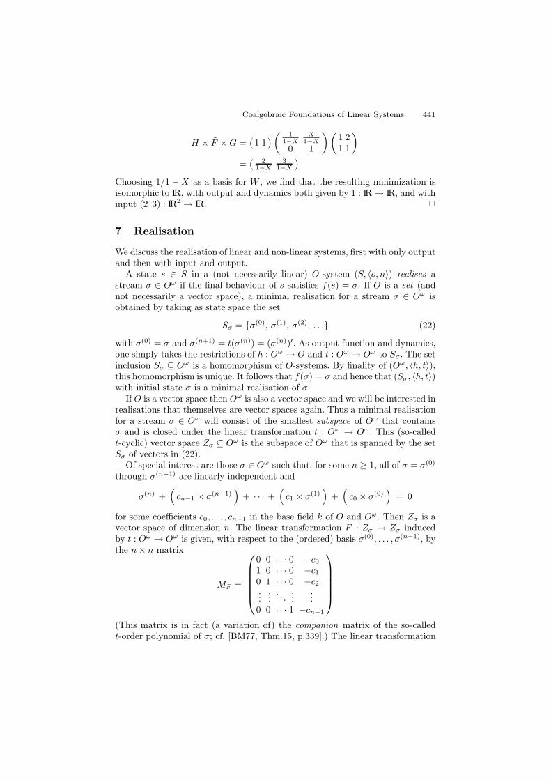
Of special interest are those σ ∈ Oω such that, for some n ≥ 1, all of σ = σ(0)

through σ(n−1) are linearly independent and

σ(n) +(

cn−1 × σ(n−1))

+ · · · +(

c1 × σ(1))

+(

c0 × σ(0))

= 0

for some coefficients c0, . . . , cn−1 in the base field k of O and Oω . Then Zσ is avector space of dimension n. The linear transformation F : Zσ → Zσ inducedby t : Oω → Oω is given, with respect to the (ordered) basis σ(0), . . . , σ(n−1), bythe n × n matrix

MF =

⎛

⎜⎜⎜⎜⎜⎝

0 0 · · · 0 −c01 0 · · · 0 −c10 1 · · · 0 −c2...

.... . .

......

0 0 · · · 1 −cn−1

⎞

⎟⎟⎟⎟⎟⎠

(This matrix is in fact (a variation of) the companion matrix of the so-calledt-order polynomial of σ; cf. [BM77, Thm.15, p.339].) The linear transformation

442 J.J.M.M. Rutten

H : Zσ → O induced by h : Oω → O is given, again with respect to the basisσ(0), . . . , σ(n−1), by the matrix (of size dim(O) × n)

MH =(σ(0)(0) σ(1)(0) σ(2)(0) · · · σ(n−1)(0)

)

Thus we have obtained a linear O-system (Zσ, 〈H, F 〉) of dimension n. As before,the inclusion Zσ ⊆ Oω is a homomorphism. Thus f(τ) = τ , for all τ ∈ Zσ and(Zσ, 〈H, F 〉) with σ as initial state is a minimal realisation of σ.

Example 13. Let O = IR and consider the stream σ = 1/(1 − X)2 ∈ Oω . Com-puting the successive stream derivatives of σ = σ(0), using Lemma 1, gives

σ(1) =2 − X

(1 − X)2σ(2) =

3 − 2X

(1 − X)2= −σ(0) + (2 × σ(1))

Thus σ(0) and σ(1) form a basis for Zσ. Because σ(0)(0) = 1 and σ(1)(0) = 2, wehave

MH =(1 2

)MF =

(0 −11 2

)

Now σ is realised by (Zσ, 〈H, F 〉), with σ as the initial state. Clearly, IR2 ∼=Zσ. Note that the isomorphism can also be obtained by computing the finalbehaviour f : IR2 → IRω of the O-system (IR2, 〈H, F 〉), using Proposition 5.This gives, for all (a, b) ∈ IR2,

f(a, b) = MH × MF × (a, b)

=(1 2

)×

(1−2X

(1−X)2−X

(1−X)2X

(1−X)21

(1−X)2

)×

(ab

)

which satisfies, as expected, f(1, 0) = σ and f(0, 1) = σ(1). �

Example 14. Let O = IR2 and consider the pair (τ, σ) ∈ (IRω)2 ∼= (IR2)ω , withτ = 1/(1 − 2X) and σ = 1/(1 − X)2. Computing (pairs of) stream derivatives

(τ, σ)(1) =(

21 − 2X

,2 − X

(1 − X)2

)(τ, σ)(2) =

(22

1 − 2X,

3 − 2X

(1 − X)2

)

(τ, σ)(3) =(

23

1 − 2X,

4 − 3X

(1 − X)2

)= 2 × (τ, σ)(0) − 5 × (τ, σ)(1) + 4 × (τ, σ)(2)

we see that Z(τ,σ) has dimension 3 with H : Z(τ,σ) → IR2 and F : Z(τ,σ) → Z(τ,σ)given by

MH =(

1 2 41 2 3

)MF =

⎛

⎝0 0 21 0 −50 1 4

⎞

⎠

�


Proposition 15. Let k be a field and let O = km. A vector of streams σ ∈(kω)m ∼= (km)ω is realisable by a linear km-system of finite dimension iff σ ∈(Rat(kω))m.

Proof : From left to right, this is Proposition 5. For the converse, it is sufficientto observe that the examples above generalise to arbitrary vectors of rationalstreams. This is immediate from the fact that for a rational stream σ = ρ/τ , thedimension of Zσ in the construction above is bounded by the maximum of thedegrees of ρ and τ . �

Next we turn to systems with input and output . Let I and O be sets. A state sin a (not necessarily linear) (I, O)-system (S, φ) realises a causal stream func-tion g : Iω → Oω if the final behaviour of s satisfies f(s) = g. For a given g,a (minimal) realisation is obtained by taking the smallest subsystem S of the fi-nal (I, O)-system (Γ, γ) containing g. The system S can be constructed by addingto the singleton set {g} all successive stream function derivatives gi, (gi)j , etc. (fori, j, . . . ∈ I), and taking the restriction of γ to S. The inclusion S ⊆ Γ is a homo-morphism of (I, O)-systems and by finality we have f(g) = g. In [Rut06, HCR06],this approach is systematically applied to the realisation (synthesis) of various(non-linear) causal functions on bitstreams (with I = O = {0, 1}).

For infinite I and O, this construction will in general not be finitely com-putable. However, if both I and O are finite dimensional vector spaces thenthe realisation of linear causal stream functions can simply be reduced to therealisation problem of streams, which we have already solved above.

Proposition 16. Let k be a field and let I = kl and O = km. Let g : (kω)l →(kω)m be given by g(τ) = M ×X × τ , for an m× l matrix M ∈ (kω)m×l. Then gis realisable by a linear (I, O)-system of finite dimension iff M ∈ (Rat(kω))m×l.

Proof: From left to right, this is Proposition 9. For the converse, we first considerthe case that l = 1. So assume that M ∈ (Rat(kω))m. By Proposition 15, thereexists a finite dimensional system (V, 〈H, F 〉) and v ∈ V realising M ; that is,f(v) = MH × MF × v = M . If we define G : k → V by the matrix MG = v then(V, Φ〈H,F,G〉) with 0 ∈ V as initial state realises g since, for all τ ∈ kω,

f(0)(τ) = MH × MF × MG × X × τ [Proposition 9]= MH × MF × v × X × τ

= M × X × τ

= g(τ)

For l > 1 we write M as a direct sum (product) M = M1 ⊕ · · · ⊕ Ml, withMi ∈ (Rat(kω))m, for i = 1, . . . , l. Then we construct realisations for each ofgi = Mi × X . Their direct sum is a realisation for g. �

444 J.J.M.M. Rutten

Acknowledgments. Discussions with Albert Benveniste – on [Rut05, Ben06]– were very instructive and are gratefully acknowledged. Thanks are also dueto Jiri Adamek, H.Peter Gumm, Jan Komenda, Prakash Panangaden, Hans-E.Porst, and Jan van Schuppen, for discussions and pointers to the literature. I amalso very grateful to the constructive comments of the three anonymous referees.Amongst others, their suggestions for improvements of the notation were veryuseful.

References

[AM74] Arbib, M.A., Manes, E.G.: Foundations of system theory: decomposablesystems. Automatica 10, 285–302 (1974)

[AM75] Arbib, M.A., Manes, E.G.: Adjoint machines, state-behaviour machines, andduality. Journal of Pure and Applied Algebra 6, 313–344 (1975)

[Ben06] Benveniste, A.: A brief on realisation theory for linear systems (unpublishednote)

[BM77] Birkhoff, G., MacLane, S.: A survey of modern algebra, 4th edn. MacMillanPublishing Co., Inc. (1977)

[Eil74] Eilenberg, S.: Automata, languages and machines. In: Pure and appliedmathematics, vol. A, Academic Press, London (1974)

[Fuh96] Fuhrmann, P.A.: A polynomial approach to linear algebra. Springer, Berlin(1996)

[HCR06] Hansen, H., Costa, D., Rutten, J.J.M.M.: Synthesis of Mealy machines usingderivatives. In: Proceedings of CMCS 2006. ENTCS, vol. 164(1), pp. 27–45.Elsevier, Amsterdam (2006)

[Kai80] Kailath, T.: Linear systems. Prentice-Hall, Englewood Cliffs (1980)[Kal63] Kalman, R.E.: Mathematical description of linear dynamical systems. SIAM

J. Control 1, 152–192 (1963)[KFA69] Kalman, R.E., Falb, P.L., Arbib, M.A.: Topics in mathematical system the-

ory. McGraw-Hill, New York (1969)[Koh78] Kohavi, Z.: Switching and finite automata theory. McGraw-Hill, New York

(1978)[Lah98] Lahti, B.P.: Signal Processing & Linear Systems. Oxford University Press,

Oxford (1998)[Pap03] Pappas, G.J.: Bisimilar linear systems. Automatica 39, 2035–2047 (2003)[Rut03] Rutten, J.J.M.M.: Behavioural differential equations: a coinductive calculus

of streams, automata, and power series (Fundamental Study). TheoreticalComputer Science 308(1), 1–53 (2003)

[Rut05] Rutten, J.J.M.M.: A tutorial on coinductive stream calculus and signal flowgraphs. Theoretical Computer Science 343(3), 443–481 (2005)

[Rut06] Rutten, J.J.M.M.: Algebraic specification and coalgebraic synthesis of Mealyautomata. In: Proceedings of FACS 2005. ENTCS, vol. 160, pp. 305–319.Elsevier Science Publishers, Amsterdam (2006)

[Son79] Sontag, E.D.: Polynomial response maps. Lecture Notes in Control and In-formation Sciences, vol. 13. Springer, Heidelberg (1979)

[vdS04] van der Schaft, A.J.: Equivalence of dynamical systems by bisimulation.IEEE Transactions on Automatic Control 49, 2160–2172 (2004)


Appendix: A Comparison with Algebraic System Theory

In the wide area of (linear) system theory, our coalgebraic treatment of linearsystems is probably closest related to what sometimes is called algebraic systemtheory. Below we give a brief overview of the approach of Kalman, who wasone of the early contributors, and compare it to the present model. Classicalreferences are [Kal63, KFA69], but see also [Kai80, Fuh96, Ben06]. Here we relyon the more categorical account of Kalman’s model described in [AM74, AM75].

Let

I(ω) = {σ ∈ Iω | σ = (i0, i1, . . . , ik, 0, 0, 0, . . .) for some k ≥ 0, ij ∈ I }

and consider the following diagram of vector spaces and linear maps:

I

e

��

G

��

��

�� O

I(ω)

X×(−)

��

r �� V

F

��

o ��

H

��Oω

t

��

h

��

I(ω)r

�� V o�� Oω

(with e(i) = (i, 0, 0, 0, . . .).) The diagram can be viewed as a theorem stating thatevery choice of linear transformations G and F induces a unique reachability mapr such that the left half of the diagram commutes, and similarly, every choiceof F and H induces a unique observability map o fitting in the right half of thediagram. In this manner, every linear system (V, H, F, G) induces a unique map(called the transfer function) o ◦ r : I(ω) → Oω . It satisfies (in our notation)

o ◦ r(σ) = H × F × r(σ) (23)

where the state r(σ) reached on input σ = (i0, i1, . . . , ik, 0, 0, . . .) ∈ I(ω) is givenby

r(σ) =(

F × G × σ)

(k)

= G(i0) + F ◦ G(i1) + F 2 ◦ G(i2) + · · · + F k ◦ G(ik)

(Note that the operational interpretation is that ik is the first input and i0 is thelast.) Comparing (23) with the final behaviour of V given in Theorem 8, we notethe following differences: (i) The final behaviour allows arbitrary input streams,not only almost-everywhere-zero ones. (ii) The ordering of the inputs coincideswith the input order. (iii) In (23), the behaviour of V is described in two steps:first r computes the state that is reached on finite input, then the (infinite)output stream is computed; in contrast, Theorem 8 describes the behaviour ofan arbitrary initial state for all (infinite) streams of inputs.

446 J.J.M.M. Rutten

Further differences between the two approaches can be noted regarding theway realisation is handled. In Kalman’s approach, a realisation of a linear mapg as in Proposition 16 is obtained by constructing its so-called (infinite) Hankelmatrix Hg, viewing Hg as a linear transformation from I(ω) to Oω , and theobservation that if Hg has finite rank then this linear transformation factorsthrough a finite dimensional vector space V as in the diagram above. In contrast,Proposition 16 reduces realisation of linear maps to the realisation of streams,and the latter are simply given by the corresponding (t-cyclic) subspaces of Oω .

coalgebraic foundations of linear systems

Documents