coaxial p h t dielectric characterizatio
TRANSCRIPT

COAXIAL PROBE FOR HIGH TEMPERATURE
DIELECTRIC CHARACTERIZATIO
by
Michael Dante Grady
A thesis submitted to the Graduate Faculty of
Auburn University
in partial fulfillment of the
requirements for the Degree of
Master of Science
Auburn, Alabama
August 9, 2010
Keywords: open-ended coaxial probe, spring-loaded probe
high temperature measurement, reflection coefficient, permittivity
Copyright 2010 by Michael Dante Grady
Approved by
Stuart Wentworth, Chair, Associate Professor of Electrical Engineering
Robert Dean, Assistant Professor of Electrical Engineering
Hulya Kirkici, Associate Professor of Electrical Engineering
Lloyd Riggs, Professor of Electrical Engineering

ii
ABSTRACT
Wireless technologies have become an integral part in how we coexist on a daily
basis. Specifically, the use of antenna systems plays a huge role in our daily lives. These
antenna systems are largely used in some form for most all modern day cellular and radar
applications. For proper construction of antenna systems, the electromagnetic properties
of the material surrounding the antennas, in particular, the material’s complex
permittivity and permeability, must be thoroughly known. It is also important to note that
the antennas will be subject to diverse temperature environments, so it is beneficial to
know how the antenna material’s electromagnetic properties will change with
temperature.
This thesis describes the design and construction of a spring-loaded stainless steel
open-ended coaxial probe used to find the electromagnetic properties of materials at
elevated temperatures. This research uses network analyzer measurements of the
reflection coefficient on an open-ended coaxial sensor in contact with a material.
Permittivity is then extracted from the reflection coefficient data by the use of a lumped
equivalent circuit model of the sensor’s fields fringing into a sample. Computer
verification of the technique is demonstrated, and results for two materials at a frequency
range between 0.5 GHz - 1.8 GHz are measured at room temperature, 45 °C, 75 °C, and
100 °C.

iii
ACKNOWLEDGMENTS
I would first like to give thanks to our Lord and savior because without him this
would not have been possible.
To my mother, Vanessa Grady, sister, Vanesia Grady, and father, Samuel Adams,
for believing in the youngest child.
To the rest of my family and friends for encouraging and helping me out in my
times of need.
To my advisor, Dr. Stuart Wentworth, for his motivating teaching style and giving
me this opportunity to contribute to the academic community.
To my Thesis Committee for their input and also helping make this transition a
smooth one.
To Dr. Overtoun Jenda, Dr. Florence Holland, and the NSF Bridge to Doctorate
Fellowship for providing a means for me to have a support system and excel throughout
my Masters education.
To Dr. Shirley Scott-Harris for putting up with me for all these years and
genuinely caring about my future.
To Calvin Cutshaw, Mike Palmer, Jim Lowry, and Linda Baressi for helping with
the fabrication of our coaxial probe.
And lastly, to anyone else I may have forgotten while writing this……Thank you!
iv
TABLE OF CONTENTS
ABSTRACT .......................................................................................................................... ii
ACKNOWLEDGMENTS ........................................................................................................ iii
LIST OF TABLES ............................................................................................................... viii
LIST OF FIGURES ................................................................................................................ ix
CHAPTER 1: INTRODUCTION ...............................................................................................1
1.1 Motivation ..........................................................................................................1
1.2 Survey of Measurement Techniques ..................................................................2
1.2.1 Freespace.............................................................................................2
1.2.2 Transmission Line ...............................................................................3
1.2.3 Resonant Cavity ..................................................................................4
1.2.4 Parallel Plate ......................................................................................5
1.2.5 Coaxial Probe ......................................................................................6
1.3 Open-Ended Coaxial Probe for Elevated Temperature Measurements .............6
1.4 Presented Coaxial Probes ...................................................................................7
1.4.1 RF Coaxial Connector Test Probe ......................................................8
1.4.2 Stainless Steel Probe ...........................................................................8
1.4.3 Spring-loaded Stainless Steel Probe ...................................................8
1.5 Looking Ahead...................................................................................................9
CHAPTER 2: OPEN-ENDED COAXIAL PROBE THEORY ......................................................10

v
2.1 Lumped Equivalent Circuit Model ..................................................................11
2.1.1 Importance of Reference Material in the Lumped Equivalent Circuit
Model ................................................................................................15
2.1.2 Finding capacitances in the probe and sample ..................................15
CHAPTER 3: TECHNIQUE VERIFICATION ...........................................................................17
3.1 Computer Results .............................................................................................17
CHAPTER 4: COAXIAL PROBES .........................................................................................21
4.1 RF Coaxial Connector Test Probe ...................................................................21
4.1.1 Fabrication of RF Coaxial Connector Test Probe .............................22
4.1.2 RF Coaxial Connector Test Probe Geometry ...................................23
4.1.3 RF Coaxial Connector Test Probe Room Temperature Setup ..........24
4.1.4 Calibration of RF Coaxial Connector Test Probe .............................25
4.1.5 Measured Results from RF Coaxial Connector Test Probe ..............27
4.1.6 Repeatability of Measurement Procedure .........................................31
4.1.7 Motivation of RF Coax Connector Test Probe Measurements on SS
Probe .................................................................................................32
4.2 Stainless Steel Probe ........................................................................................33
4.2.1 Stainless Steel Probe for Elevated Temperature Measurements.......33
4.2.2 Construction of Stainless Steel Probe ...............................................34
4.2.3 Stainless Steel Probe Geometry ........................................................35
4.2.4 Stainless Steel Probe Room Temperature Setup ...............................35
4.2.5 Calibration of the Stainless Steel Probe ............................................37
4.2.6 Measured Results from Stainless Steel Probe ...................................37

vi
4.2.7 Motivation of Stainless Steel Probe Measurements on Spring-loaded
Stainless Steel Probe .........................................................................38
4.3 Spring-loaded Stainless Steel Probe ................................................................39
4.3.1 Construction of Spring-loaded Stainless Steel Coaxial Probe ..........39
4.3.2 Spring-loaded Stainless Steel Coaxial Probe Geometry ...................41
4.3.3 Spring-loaded Stainless Steel Probe Room Temperature Setup .......41
4.3.4 Calibration of the Spring-loaded Stainless Steel Probe ....................41
4.3.5 Measured Results from Spring-loaded Stainless Steel Probe ...........42
CHAPTER 5: COAXIAL PROBE FOR HIGH TEMPERATURE DIELECTRIC
CHARACTERIZATION ...................................................................................................45
5.1 Spring-loaded Stainless Steel Probe Elevated Temperature Setup ..................45
5.2 Calibration of the Spring-loaded Stainless Steel Probe for Elevated
Temperatures....................................................................................................47
5.3 Measured Results from Spring-loaded Stainless Steel Probe for Elevated
Temperatures....................................................................................................48
CHAPTER 6: CONCLUSIONS ...............................................................................................54
6.1 Technique Summary ........................................................................................54
6.2 Future Work .....................................................................................................55
6.2.1 Numeric solution for an open-ended coaxial probe .........................56
6.2.2 Calibration Standards ........................................................................60
6.2.3 Gold Plated Probe .............................................................................61
6.3 Conclusions ......................................................................................................65

vii
REFERENCES ....................................................................................................................66
APPENDIX A: CALIBRATION STANDARDS OVERVIEW ......................................................69
A.1 Open Calibration Standard ..............................................................................69
A.2 Short Calibration Standard ..............................................................................70
A.3 Load Calibration Standard ..............................................................................72
APPENDIX B: TECHNIQUE DETAILS ................................................................................79
B.1 Room Temperature Measurement Procedure ..................................................79
B.2 Elevated Temperature Measurement Procedure .............................................82
A.3 Load Calibration Standard ..............................................................................72
APPENDIX C: MATLAB CODE .......................................................................................87
C.1 Lump Equivalent Circuit Model Code ............................................................87
C.1.a 1-Port De-embedding Algorithm ...................................................89
C.2 Numerical Method Extraction Code ...............................................................91

viii
LIST OF TABLES
Table 3.1 Computer Simulation Measurement Schematic ..............................................20
Table 4.1 Test Probe Properties .......................................................................................24
Table 4.2 Relative Permittivity Value for Full S11 Calibration Material Combo
(test probe) .......................................................................................................28
Table 4.3 Relative Permittivity Value for Response Calibration (test probe) .................30
Table 4.4 Stainless Steel Probe Properties .......................................................................35
Table 4.5 Relative Permittivity Value for Calibration Material Combinations (SS probe) .
..........................................................................................................................37
Table 4.6 Spring-loaded Stainless Steel Probe Properties ...............................................41
Table 4.7 Relative Permittivity Value for Calibration Material Combinations (Spring-
loaded)..............................................................................................................42
Table 4.8 Relative Permittivity Value for Response Calibration (Spring-loaded probe)
..........................................................................................................................43
Table 5.1 Relative Permittivity Value for Full-S11 Calibration (SL probe) ...................49
Table 5.2 Relative Permittivity Value for Response Calibration (SL probe) ..................51
Table 6.1 Thermal and Electrical Conductivities of Gold and Stainless .........................61
Table 6.2 Calculations of Heat Conducted by Gold Plated probe ...................................64

ix
LIST OF FIGURES
Figure 1.1 Free-space pyramidal horn antennas measuring a material ...............................3
Figure 1.2 Coaxial and waveguide transmission line .........................................................4
Figure 1.3 Rectangular waveguide cavity resonator ...........................................................4
Figure 1.4 Parallel plate capacitor with air (left) and parallel plate capacitor with
dielectric material (right) ...................................................................................5
Figure 1.5 Coaxial Probe made from RF connector ...........................................................6
Figure 2.1 Cross-section of open-ended coaxial probe .....................................................10
Figure 2.2 Open-ended coaxial probe in contact with material (left) and lumped
equivalent circuit model of an open-ended coaxial probe (right) ...................11
Figure 2.3 Cutoff wavelengths of the TM and TE modes in a coaxial line. .....................12
Figure 2.4 Field distributions of the principal TEM and lower order TE and TM modes
in a coaxial line ................................................................................................13
Figure 3.1 ADS Schematic of Calibration ........................................................................18
Figure 3.2 ADS Schematic of Measurement Process .......................................................19
Figure 4.1 NMale to SMAMale RF coaxial adapter ..............................................................22
Figure 4.2 RF coaxial test probe made from NMale to SMAMale RF coaxial adapter ...22
Figure 4.3 Cross-section of a coaxial line .........................................................................22
Figure 4.4 Agilent HP-4396B VNA .................................................................................24
Figure 4.5 Measurement Materials for test probe at room temperature ...........................25

x
Figure 4.6 Test probe placed against a material during extraction ...................................25
Figure 4.7 Measured value of Polycarbonate using the “Short” Response Calibration
(brass) ...............................................................................................................31
Figure 4.8 Relative Permittivity Value (Real vs Imaginary) for Tivar of Eight Separate
Measurements using the Air, brass, 50 Ω AR Calibration Combination .....32
Figure 4.9 Stainless Steel Probe........................................................................................34
Figure 4.10 Measurement Materials for Stainless Steel Probe at room temperature .......36
Figure 4.11 Stainless Steel probe held with gripper during extraction .............................36
Figure 4.12 Stainless Steel probe placed against a material during extraction .................36
Figure 4.13 Makeup of Spring-loaded Stainless Steel Probe ...........................................39
Figure 4.14 Spring-loaded Stainless Steel Probe ..............................................................40
Figure 4.15 Measured value of Polyethylene using the “Open” Response Calibration
(air) ................................................................................................................44
Figure 5.1 Stainless Steel probe high temperature measurement setup ...........................46
Figure 5.2 Stainless Steel probe placed against a material during high temperature
testing .............................................................................................................47
Figure 5.3 Relative Permittivity Extraction of Tivar at four temperatures using the
Room Temperature Full S11 Calibration .......................................................50
Figure 5.4 Relative Permittivity Extraction of Teflon at four temperatures using the
Room Temperature Full S11 Calibration .......................................................51
Figure 5.5 Relative Permittivity Extraction of Tivar at four temperatures using the
Response Calibration ......................................................................................52
xi
Figure 5.6 Relative Permittivity Extraction of Teflon at four temperatures using the
Response Calibration ......................................................................................53
Figure 6.1 Open-ended coaxial probe in contact with material of relative complex
permittivity, εr ..................................................................................................57
Figure 6.2 The probe tip geometry defining Equation (2.8). ............................................58
Figure A.1 Styrofoam brand rectangular sheet .................................................................70
Figure A.2 Brass plate.......................................................................................................70
Figure A.3 Steel plate from rectangular waveguide .........................................................71
Figure A.4 Short Standard connected at end of coaxial connector plumbing ..................71
Figure A.5 Liquid used as Short Standard ........................................................................72
Figure A.6 50 Ω Annular Resistor ....................................................................................73
Figure A.7 Annular resistor ..............................................................................................74
Figure A.8 Load Standard connected at end of coaxial connector plumbing ...................77
Figure A.9 Liquid used as Load Standard ........................................................................77
Figure A.10 Square Resistor .............................................................................................78

1
CHAPTER 1
ITRODUCTIO
1.1 Motivation
Most modern day communication technology employs an antenna system within
its overall system design. For example, cell phone base stations make use of several
antennas mounted on a cell tower to transmit and receive wireless signals. Likewise,
many radar systems achieve the transmission and reception of wireless signals with the
use of an aboveground directional antenna. These communication infrastructures are very
practical, but are extremely vulnerable to natural disasters, vandalism, and terrorism [1].
Due to the consequences resulting from an antenna’s destruction, it is critical to find an
alternative means for transmitting and receiving wireless signals.
Subsurface antenna systems for cellular and radar applications may provide a
robust alternative to aboveground antennas. One type of subsurface antenna is the
geotextile antenna, consisting of electrically conductive structures containing electronic
transmission and reception materials within its fibers. For proper construction, the
electromagnetic properties of the material surrounding the antennas, in particular, the
material’s complex permittivity and permeability, must be thoroughly known [1]. It is
also important to note that the antennas will be subject to diverse temperature

2
environments, so it is beneficial to know how the antenna material’s electromagnetic
properties will change with temperature.
At present, most materials are characterized at room temperature, and there is
rather limited data regarding how the electromagnetic properties change with high
temperatures. This principal concern is the motivation for the presented work.
1.2 Survey of Measurement Techniques
There are five common measurement techniques used to find a material’s
complex permittivity and permeability [2]. Among these are the Free-space,
Transmission line, and Resonant cavity methods which can be used to simultaneously
calculate a material’s permittivity and permeability. In contrast, the Parallel plate and
Coaxial probe techniques are well suited to calculate the permittivity of a material. A
brief description and illustration of each procedure is described below.
1.2.1 Free-space
The free-space method involves using measures of reflection and transmission to
extract electrical and magnetic properties. Measurements can be taken using a vector
network analyzer. As shown in Figure 1.1, this method makes use of horn antennas as
transmitters and receivers on opposite sides of the material under test. The measured
received signal allows calculation of permittivity [3]. The free-space method uses either a
TRL (thru, reflect, line) or TRM (thru, reflect, match) calibration technique to remove
reflection errors [3, 4]. This method can be used for a variety of frequency ranges. The
limiting factor for the frequency range is the horn dimensions. A few advantages of this

3
method are that it requires no direct contact to the materials and there are no special
machining requirements for the materials. These advantages therefore make it a good
choice for high temperature measurements [5]. A few main drawbacks to this method are
that it requires using a large cross sectional area of the material in order to achieve
accurate results and that the frequency response is limited by the waveguide.
1.2.2 Transmission Line
The transmission line methods use reflection and transmission measurements to
extract both electrical and magnetic properties, and are achieved by placing a material
inside an enclosed segment of transmission line [3]. Measurements are taken with a
network analyzer and either a coaxial line or a rectangular waveguide as depicted in
Figure 1.2. The transmission line method can be executed by using either a one or two-
port system. Coaxial lines and rectangular waveguides are primarily utilized when using
a two port system. The one-port system involves placing a sample in a line terminated by
a known load [6]. This transmission line method is widely regarded as one of the simpler
ways to extract permittivity and permeability. This method can be used for a variety of
Figure 1.1 Free-space pyramidal horn antennas measuring a material

4
frequency ranges. The limiting factor for the frequency range is the transmission line
dimensions. The key disadvantages to this method are that materials must be precisely
machined to fit the test fixture, and air gaps at fixture walls will cause inaccuracies. Also,
while coaxial line samples are harder to construct than waveguide samples, they can be
used over a much wider frequency range.
1.2.3 Resonant Cavity
The resonant cavity
method uses a cavity fixture to
measure the quality factor and
center frequency, parameters
which are perturbed when a
material is placed in the cavity. The
changes in these values are then
related to either or both the permittivity and permeability at a single frequency [3].
Measurements from the resonant cavity method can be taken with a network analyzer and
stripline or waveguide resonator cavities. The stripline resonator cavity consists of a
Figure 1.2 Coaxial and waveguide transmission line (Taken from [8] )
Figure 1.3 Rectangular waveguide cavity resonator
(Taken from [8] )

5
center-strip conductor mounted equidistantly between two ground planes and terminated
by two end plates [7]. The waveguide resonator cavity can either be a rectangular (in
Figure 1.3), circular, or elliptical waveguide terminated with plates at ends of the
waveguide. This method can only be used for a single frequency. The limiting factor for
this single frequency is the cavity dimensions. The resonant cavity method is considered
to be the most accurate technique among techniques to find both electrical and magnetic
properties. One disadvantage is that measurements can only be taken at a single
frequency.
1.2.4 Parallel Plate
The parallel plate method
involves using parallel plate capacitor
theory. It consists of inserting a
dielectric material in between two
conducting plates [9]. When the sample
is in the parallel plate arrangement,
the capacitance is related exactly to
the geometry and the permittivity [3].
Measurements are taken using a LCR
meter or an impedance analyzer. Permittivity measurements can then be made by finding
the ratio of the capacitance of the parallel plates with the space between the plates filled
with the dielectric to the capacitance with the space being air [10] as depicted in Figure
1.4. The usable frequency range is determined by both the dimensions of the conducting
Figure 1.4 Parallel plate capacitor with air (left) and
parallel plate capacitor with dielectric material (right)
(Picture taken from http://www.physics.sjsu.edu/...
becker/physics51/capacitors.htm)

6
plate and the dimensions of the tested material. A few advantages to this method are its
low-cost assembly and reasonably simple calculation of permittivity. This method is also
well suited for thin flat materials. One main disadvantage to this method is that the charge
density at the edges becomes larger as compared to the charge density in the center. This
increased charge density causes the measured permittivity to appear larger than the actual
value.
1.2.5 Coaxial Probe
The coaxial probe technique
involves finding a material’s
permittivity by taking reflection
coefficient measurements with an open-
ended coaxial probe. The typical
measurement system includes a
network analyzer and a coaxial probe.
The open-ended coaxial probe is a cut-off section of transmission line, as shown in Figure
1.5, which is brought in contact with the tested material such that the fields at the probe
end fringe into the material. After the correct arrangement is achieved, the reflection data
can then be related to permittivity because the fringing fields change as they come in
contact with the tested material. This type of one-port measurement requires a three term
calibration technique to ensure validity of acquired data. The usable frequency range is
determined by both the dimensions of both the outer and inner conductors. The coaxial
probe technique is suitable for taking measurements of multiple samples, liquids, and
Figure 1.5 Coaxial Probe made from RF connector

7
planar solids. A few constraints to this method are that air gaps can cause significant
errors, and it is not well-matched for materials with both electrical and magnetic losses.
This technique is very attractive because of its non-destructive nature and the ease of
sample preparation [3].
1.3 Open-Ended Coaxial Probe for Elevated Temperature Measurements
For robust, real world antenna design, it is beneficial to investigate how a
material’s electromagnetic properties change with temperature. In order to determine this,
a measurement system that will withstand elevated temperatures must be developed.
Open-ended coaxial probes are very attractive for taking high temperature measurements
because the technique is a one-port measurement that does not require much sample
preparation and offers a relatively simple user interface to an enclosed heating space. For
this reason, an open-ended coaxial probe with properly selected fabrication materials is a
superior measurement system for tackling the pre-stated problem. This work is
demonstrated for temperatures up to 100°C.
1.4 Presented Coaxial Probes
In this work, three open-ended coaxial probes are presented. All probes are used
to find the complex permittivity of dielectric materials at room temperatures, and one is
used for elevated temperature measurements. The probes are brought in contact with the
tested material such that the fields at the probe end fringe into the material. After this
arrangement is formed, complex permittivity is then extracted. The first probe or test
probe is made from a highly polished-machined RF coaxial connector. The second probe

8
(called the stainless steel probe) is made from a stainless steel rod and pipe and a RF
Clamp Type Connector. The third probe or spring-loaded stainless steel probe is a
variation of the original stainless steel probe designed for measurement at elevated
temperatures. All measurements are taken for a frequency range of 0.5 GHz to 1.8 GHz.
1.4.1 RF Coaxial Connector Test Probe
The open-ended coaxial connector test probe was made from a highly polished-
machined NMale to SMAMale RF coaxial connector. It is used to extract the complex
permittivity of materials at room temperature. The RF coaxial connector test probe served
as a baseline for the measurements taken. It was also the basis for the fabrication and
testing of the stainless steel probe at room temperature.
1.4.2 Stainless Steel Probe
The stainless steel open-ended coaxial air probe is made from a stainless steel
pipe and a stainless steel cylindrical rod connected to a RF NMale Clamp Type Connector.
The design and measurement results are compared with the room temperature
measurement results obtained from the RF coaxial connector test probe. The weaknesses
and measurement difficulty of this version of the stainless steel probe were the basis for
the design and implementation of a spring- loaded coaxial probe.
1.4.3 Spring-loaded Stainless Steel Probe
This probe is a variation of the original stainless steel open-ended coaxial air
probe which is made from a stainless steel pipe and a stainless steel cylindrical rod
9
connected to a RF NMale Clamp Type Connector. This probe enhanced the original probe
setup with the addition of a spring-loaded mechanism. It is ultimately used to extract the
complex permittivity of materials at elevated temperatures. The spring-loaded stainless
steel coaxial probe is demonstrated with temperatures as high as 100° C.
1.5 Looking Ahead
Chapter 2 describes the theory behind the open-ended coaxial probe method. The
lumped equivalent circuit model of the probe’s fields fringing into a sample modeling
methods is presented. In Chapter 3, the open-ended coaxial probe technique is verified by
computer simulation. Chapter 4 explains the construction, calibration, and measurement
results obtained from the RF coaxial connector test probe. It alludes to how the acquired
results motivate the construction and testing of the stainless steel coaxial probe. Chapter 4
also discusses the construction, calibration, and measurement results obtained from the
stainless steel probe. It then describes how these results motivate the creation of a spring-
loaded stainless steel coaxial probe. Lastly, Chapter 4 discusses the construction and
calibration obtained from the spring-loaded stainless steel probe. The room temperature
results obtained from the spring-loaded stainless steel coaxial probe are then explored.
This chapter also tells about how the spring-loaded stainless steel coaxial probe will be
used for high temperature measurements. In Chapter 5, the elevated temperature
calibration and results are presented. These results are then compared to the room
temperature results obtained from the spring-loaded stainless steel coaxial probe. Chapter
6 concludes with discussion on the advantages and disadvantages of each probe. This
chapter also presents future improvements to the calibration and extraction procedures.

10
CHAPTER 2
OPE-EDED COAXIAL PROBE THEORY
The open-ended coaxial probe is a
form of cut-off section of a transmission line
that, like any other coaxial line, contains a
center conductor of radius ‘a’ surrounded by
some dielectric material with relative
permittivity, εrp, all of which is enclosed by
an outer conductor of radius ‘b’ as depicted
in Figure 2.1. The expression “coaxial”
comes from the inner and outer conductor
sharing a common axis. Measurements from the coaxial probe are acquired by placing the
end of the probe in contact with a material, so that the fields at the probe end fringe into
the material and return reflection data measurements. The probe’s measured data presents
a challenge in calculating the dielectric constant because there is no readily
acknowledged analytical relationship between the reflection coefficient and permittivity.
There are several models for an open-ended coaxial probe. A number of these
models give an expression for the admittance as a function of the dielectric constant.
One of the most attractive modeling methods was employed: a lumped equivalent circuit
Figure 2.1 Cross-section of open-ended coaxial probe

11
model of the probe’s fields fringing into a sample. This model is attractive because it is
one of the simplest algorithms to implement.
2.1 Lumped Equivalent Circuit Model [12]
The lumped equivalent circuit model can be used when an open coaxial line,
placed in contact with a test sample (Figure 2.2), is used as a sensor. The tested sample
must be homogeneous within a volume sufficiently large to simulate a semi-infinite slab.
A semi-infinite slab means that the tested sample thickness should allow the magnitude
of the electric field at the far end of the sample to be at least two orders smaller than that
at the probe to sample interface. If this condition is satisfied, the discontinuity at the
termination of the coaxial line can be modeled by an equivalent lumped circuit. This
discontinuity, in the absence of a lossy dielectric, is frequently assumed to be purely
capacitive and to consist of two elements: a capacitance originating from the probe's
fringing field (Cp), and a capacitance originating from the sample fringing field (Cs), as
shown in Figure 2.2.
Figure 2.2 Open-ended coaxial probe in contact with material (left) and lumped equivalent circuit model of an open-ended coaxial probe (right)
12
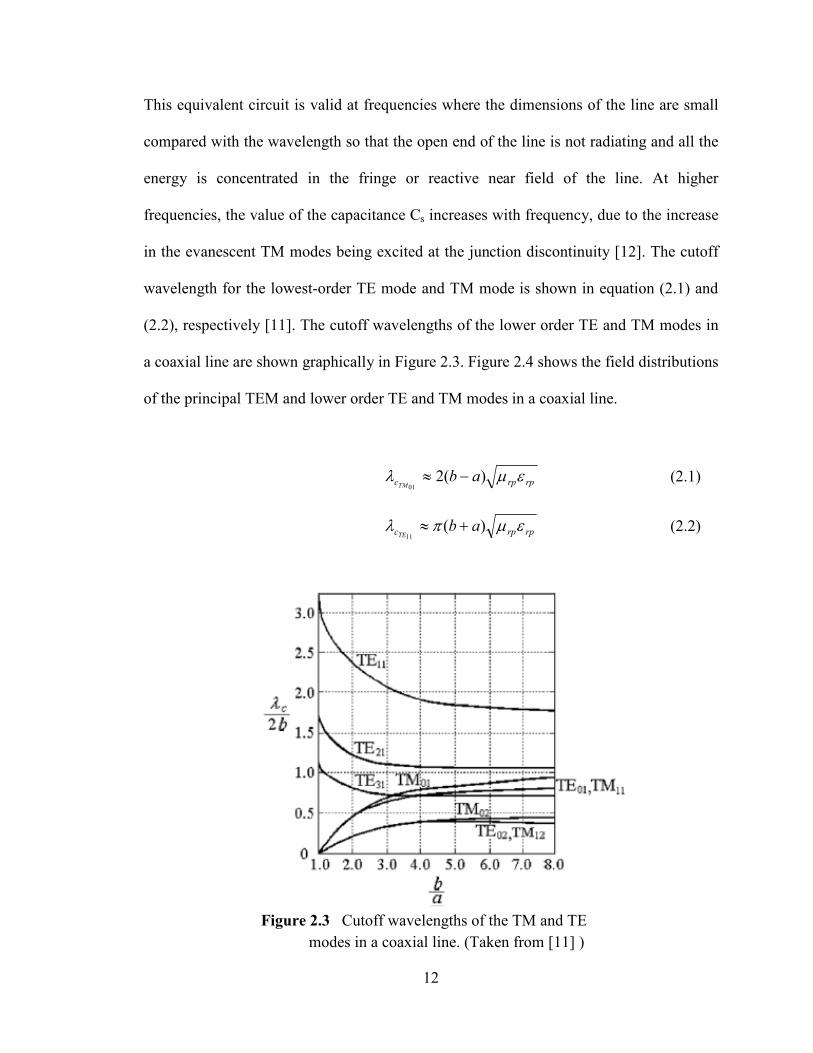
This equivalent circuit is valid at frequencies where the dimensions of the line are small
compared with the wavelength so that the open end of the line is not radiating and all the
energy is concentrated in the fringe or reactive near field of the line. At higher
frequencies, the value of the capacitance Cs increases with frequency, due to the increase
in the evanescent TM modes being excited at the junction discontinuity [12]. The cutoff
wavelength for the lowest-order TE mode and TM mode is shown in equation (2.1) and
(2.2), respectively [11]. The cutoff wavelengths of the lower order TE and TM modes in
a coaxial line are shown graphically in Figure 2.3. Figure 2.4 shows the field distributions
of the principal TEM and lower order TE and TM modes in a coaxial line.
rprpc abTM
εµλ )(201
−≈ (2.1)
rprpc abTE
εµπλ )(11
+≈ (2.2)
Figure 2.3 Cutoff wavelengths of the TM and TE modes in a coaxial line. (Taken from [11] )

13
Figure 2.4 Field distributions of the principal TEM and lower order TE and TM modes in a coaxial line (Taken from [11] )
14
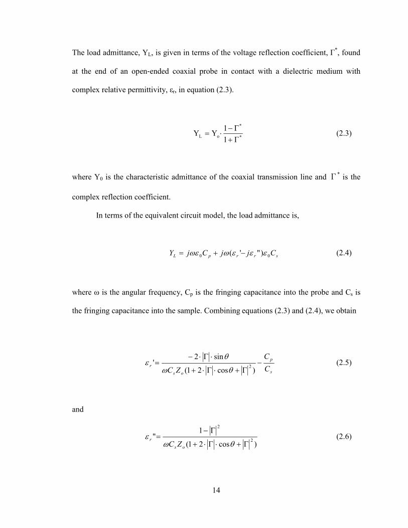
The load admittance, YL, is given in terms of the voltage reflection coefficient, Γ*, found
at the end of an open‐ended coaxial probe in contact with a dielectric medium with
complex relative permittivity, εr, in equation (2.3).
*
*
oL Γ1Γ1
YY+
−⋅= (2.3)
where Y0 is the characteristic admittance of the coaxial transmission line and 〉* is the
complex reflection coefficient.
In terms of the equivalent circuit model, the load admittance is,
srrpL CjjCjY 00 )"'( εεεωωε −+= (2.4)
where ω is the angular frequency, Cp is the fringing capacitance into the probe and Cs is
the fringing capacitance into the sample. Combining equations (2.3) and (2.4), we obtain
s
p
os
rC
C
ZC−
Γ+⋅Γ⋅+
⋅Γ⋅−=
)cos21(
sin2' 2
θω
θε (2.5)
and
)cos21(
1" 2
2
Γ+⋅Γ⋅+
Γ−=
θωε
os
r
ZC (2.6)

15
where εr’, in (2.5), and εr”, in (2.6), are the real part and the imaginary part of the relative
complex permittivity, respectively, Z0 is the characteristic impedance of the transmission
line, and 〉 is the magnitude of the complex reflection coefficient with phase angle θ
[12].
2.1.1 Importance of Reference Material in the Lumped Equivalent Circuit Model
Both the fringing capacitances in the probe, Cp, and the fringing capacitance in
the sample, Cs, are found using a reference material. The dielectrics used for the reference
material should be of known permittivity, should not be a calibration standard, and
should satisfy the optimum capacitance condition at a selected measurement frequency
(found in [13]). The calibration standards cannot be used as a reference material because
the standards are used in the error correction model as an open, a short, or a load. If any
standard is used as a reference material, this would result in a minimal change in the
magnitude and phase of the reflection coefficient obtained for the reference material, and
would result in systematic errors.
2.1.2 Finding capacitances in the probe and sample [13]
As a first approximation Cp can be assumed to be equal to zero, and either εr’ or
εr” of the reference material can be used to determine Cs. The following relationships are
employed, the first for εr’ in equation (2.7) and the second for εr” in equation (2.8):
)cos21('
sin22
refrefrefro
refref
s
ZC
Γ+⋅Γ⋅+
⋅Γ⋅−=
θεω
θ (2.7)
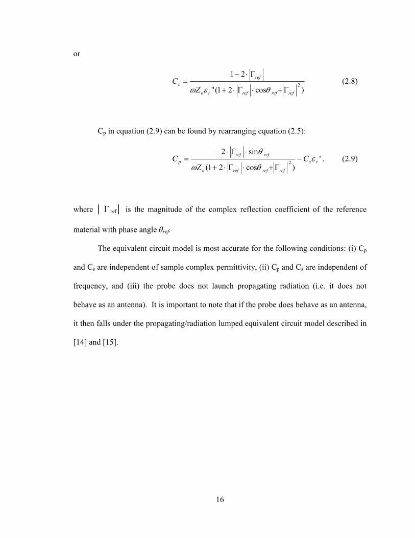
16
or
)cos21("
212
refrefrefro
ref
s
ZC
Γ+⋅Γ⋅+
Γ⋅−=
θεω (2.8)
Cp in equation (2.9) can be found by rearranging equation (2.5):
')cos21(
sin22 rs
refrefrefo
refref
p CZ
C εθω
θ−
Γ+⋅Γ⋅+
⋅Γ⋅−= . (2.9)
where 〉ref is the magnitude of the complex reflection coefficient of the reference
material with phase angle θref.
The equivalent circuit model is most accurate for the following conditions: (i) Cp
and Cs are independent of sample complex permittivity, (ii) Cp and Cs are independent of
frequency, and (iii) the probe does not launch propagating radiation (i.e. it does not
behave as an antenna). It is important to note that if the probe does behave as an antenna,
it then falls under the propagating/radiation lumped equivalent circuit model described in
[14] and [15].

17
CHAPTER 3
TECHIQUE VERIFICATIO
The extraction procedure was initially verified using Agilent Advance Design
System (ADS). The open-ended coaxial probe setup was modeled for the materials that
would eventually be tested at room temperature. Once verified with the computer results,
the procedure was used with the data gathered from an HP 4326B vector network
analyzer.
3.1 Computer Results
The simulation in Agilent’s ADS was set up in same manner it would be used in
an actual measurement. It must first be established that there are three different methods
for which to calibrate the coaxial probe. One is to use an automatic calibration, where the
calibration is done entirely by the VNA. Another is a semi-automatic calibration, where
the VNA is used to calibrate the probe and then a de-embedding procedure is applied to
obtain measurements. The last is a manual calibration, where the user manually measures
each calibration standard and uses a de-embedding procedure to extract data. This
simulation was done assuming a one-port manual calibration technique because the de-
embedding procedure is ideally identical to the extraction method used in the automatic
calibration. Data was taken from the end of an open-ended coaxial probe from a

18
reference material, a material under test, an open calibration standard, a short calibration
standard, and a load calibration standard. Figure 3.1 shows the general layout of the
calibration procedure while Figure 3.2 shows the ADS layout of the measurement
procedure. The open-ended coaxial probe is connected to an S-parameter measurement
termination and the respective measurement load. The measurement termination
represents the reference plane at the VNA. In Figure 3.1, the “Open” impedance is equal
to ∞, the “Short” has an impedance of 0 Ω, and the “Load” has an impedance of 50 Ω.
COAX_MDS
TL5
TanD=.0003
Er=2.10006
Mur=1.0
Cond2=18E6
Cond1=18E6
T=0.0 mil
L=900 mil
Ro=740 mil
Ri=396 mil
A=127 mil
Term
Term5
Z=50 Ohm
Num=5
Term
Load
Z=50 Ohm
Num=8
Term
Short
Z=.00000001e-300 Ohm
Num=7
Term
Term4
Z=50 Ohm
Num=4
COAX_MDS
TL4
TanD=.0003
Er=2.10006
Mur=1.0
Cond2=18E6
Cond1=18E6
T=0.0 mil
L=900 mil
Ro=740 mil
Ri=396 mil
A=127 mil
Term
Open
Z=1000000000000e100000000 Ohm
Num=6
COAX_MDS
TL3
TanD=.0003
Er=2.10006
Mur=1.0
Cond2=18E6
Cond1=18E6
T=0.0 mil
L=900 mil
Ro=740 mil
Ri=396 mil
A=127 mil
Term
Term3
Z=50 Ohm
Num=3
Figure 3.1 ADS Schematic of Calibration

19
In Figure 3.2, the probe first measures the reference material, Teflon with an εr value of
2.1 - j0.0003 [16], then two tested materials, Tivar with an εr value around 2.25 - j0.0007
[16] and Polycarbonate with an εr value around 2.85 - j0.003 [17]. The ADS coaxial line
component, COAX_MDS, serves as the open-ended coaxial probe with the same
geometry as the probe that will be used. The SSLIN is an ADS substrate component
serving as the material to be tested by the coaxial line. Each substrate component is made
to appear as a semi-infinite slab (by making the material thickness large as compared to
the coaxial line size) with identical dielectric properties of the material it represents.
Table 3.1 shows the calculated median values of εr from 500 MHz to 1.8 GHz for two
different material input values.
Term
Short2
Z=.00000001e-300 Ohm
Num=10
Term
Term2
Z=50 Ohm
Num=2
SSLIN
Tivar
L=2500.0 mil
W=2500.0 mil
Subst="SSSub2"COAX_MDS
TL6
TanD=.0003
Er=2.10006
Mur=1.0
Cond2=18E6
Cond1=18E6
T=0.0 mil
L=900 mil
Ro=740 mil
Ri=396 mil
A=127 mil
Term
Short3
Z=.00000001e-300 Ohm
Num=3
SSLIN
Polycarbonate
L=2500.0 mil
W=2500.0 mil
Subst="SSSub3"
Term
Term6
Z=50 Ohm
Num=6 COAX_MDS
TL7
TanD=.0003
Er=2.10006
Mur=1.0
Cond2=18E6
Cond1=18E6
T=0.0 mil
L=900 mil
Ro=740 mil
Ri=396 mil
A=127 mil
SSSUB
SSSub2
TanD=.0007
T=1000 mil
Hl=1000.0 mil
Hu=1000.00 mil
Cond=.2E-7
Mur=1
Er=2.3
H=1000 mil
SSSub
SSSUB
SSSub3
TanD=.005
T=1000 mil
Hl=1000.0 mil
Hu=1000.00 mil
Cond=.2E-7
Mur=1
Er=2.9
H=1000 mil
SSSub
SSSUB
SSSub1
TanD=.0003
T=1000 mil
Hl=1000.0 mil
Hu=1000.00 mil
Cond=10E-14
Mur=1
Er=2.1
H=1000 mil
SSSub
Term
Short1
Z=.00000001e-300 Ohm
Num=9
SSLIN
Teflon
L=2500.0 mil
W=2500.0 mil
Subst="SSSub1"COAX_MDS
TL1
TanD=.0003
Er=2.10006
Mur=1.0
Cond2=18E6
Cond1=18E6
T=0.0 mil
L=900 mil
Ro=740 mil
Ri=396 mil
A=127 mil
Term
Term1
Z=50 Ohm
Num=1
Figure 3.2 ADS Schematic of Measurement Process

20
This ADS simulation confirms that this procedure indeed works. It can be seen that there
is little difference in real component of the relative permittivity between the input and the
calculated simulation values using the lumped equivalent circuit model from Chapter 2.1.
It is also expected from this simulation that the one port measurement is not well suited
for loss tangent measurements (imaginary component of the relative permittivity).
Tivar Polycarbonate
εr’ εr” εr’ εr”
Input 2.300 0.0007 2.900 0.0050
Calculated 2.282 -2.652 E-16 2.831 -8.126 E-16
Table 3.1 Computer Simulation Measurement Schematic

21
CHAPTER 4
COAXIAL PROBES
In this work, three open-ended coaxial probes are presented. All probes are used
to find the complex permittivity of dielectric materials at room temperatures, and one is
used for elevated temperature measurements. The probes are brought in contact with the
tested material such that the fields at the probe end fringe into the material. After this
arrangement is formed, complex permittivity is then extracted. The first probe or test
probe is made from a highly polished- machined RF coaxial connector. The second probe
or stainless steel probe is made from stainless steel bars and a RF Clamp Type Connector.
The third probe or spring-loaded stainless steel probe is a variation of the original
stainless steel probe. All measurements are within a frequency range of 0.5 GHz to 1.8
GHz.
4.1 RF Coaxial Connector Test Probe
The test probe for room temperature measurements was made from a highly
polished-machined NMale to SMAMale RF coaxial connector. The N-Type coaxial
connector proved to be a practical option for the initial test probe because the N-Type
connector was manufactured with a characteristic impedance of 50 Ω (which is needed to
match the measurement system). The design restrictions and measurement results
obtained from the RF coaxial connector test probe were used as the motivation for the

22
construction of the stainless steel coaxial probe. The results from the RF coaxial
connector test probe were also used to confirm the validity of the results obtained from
the stainless steel probe at room temperature.
4.1.1 Fabrication of RF Coaxial Connector Test Probe
The test probe was fabricated from an NMale to SMAMale RF coaxial adapter
(Figure 4.1) which has a characteristic impedance of 50 Ω. A lathe was used to both
remove the outer shell of the coaxial connector and file down the center pin and
surrounding shell until the insulating material was flush with both the inner and outer
metal conductors. After achieving a flat surface, the probe end was polished using 400,
600, 1000, and 2000 grade sand paper. The finished surface of the RF coaxial connector
test probe is shown in Figure 4.2.
Figure 4.1 NMale to SMAMale RF coaxial adapter Figure 4.2 RF coaxial test probe made
from NMale to SMAMale RF
coaxial adapter
Figure 4.3 Cross-section of a coaxial line
23
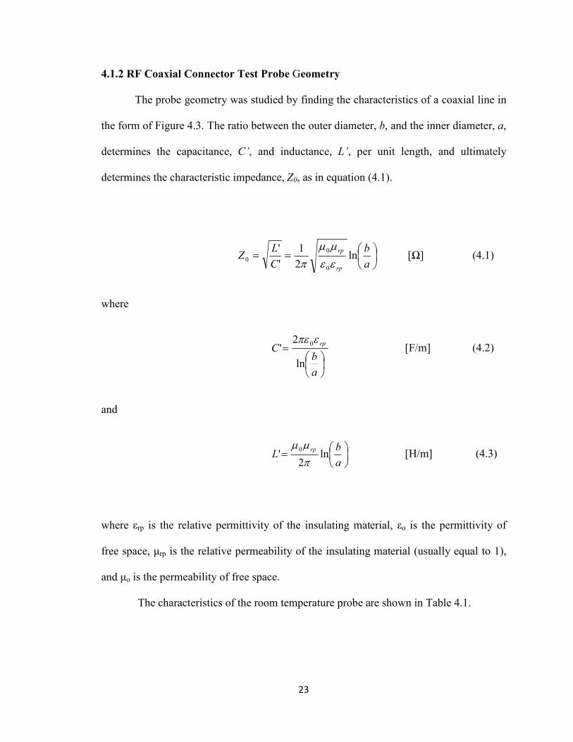
4.1.2 RF Coaxial Connector Test Probe Geometry
The probe geometry was studied by finding the characteristics of a coaxial line in
the form of Figure 4.3. The ratio between the outer diameter, b, and the inner diameter, a,
determines the capacitance, C’, and inductance, L’, per unit length, and ultimately
determines the characteristic impedance, Z0, as in equation (4.1).
==a
b
C
LZ
rp
rpln
2
1
'
'
0
0
0 εε
µµ
π [Ω] (4.1)
where
=
a
bC
rp
ln
2'
0επε [F/m] (4.2)
and
=a
bL
rpln
2'
0
π
µµ [H/m] (4.3)
where εrp is the relative permittivity of the insulating material, εo is the permittivity of
free space, µrp is the relative permeability of the insulating material (usually equal to 1),
and µo is the permeability of free space.
The characteristics of the room temperature probe are shown in Table 4.1.

24
4.1.3 RF Coaxial Connector Test Probe Room Temperature Setup
The RF coaxial connector test
probe apparatus for room temperature
measurements consists of an Agilent,
Hewitt Packard-4396B Vector Network
Analyzer (VNA) (Figure 4.4), the RF
coaxial connector test probe, the
calibration standards, the reference material,
and the material under test (Figure 4.5).
The Agilent HP-4396B VNA (description found at http://
www.testequipmentconnection.com) provides RF vector network, spectrum, and optional
impedance measurements for lab and production applications. Gain, phase, group delay,
and distortion are some of the properties that can be measured using this one instrument.
When combined with a test set, the Agilent 4396B provides reflection measurements,
such as return loss, and SWR, and S parameters.
As a vector network analyzer, the Agilent 4396B operates from 100 kHz to 1.8
GHz with 1 mHz resolution, and its integrated synthesized source provides -60 to +20
Test Probe Properties
b 1.006 cm
a 0.3226 cm
εr 2.100 (Teflon)
Zo 47.05 Ω
Table 4.1 Test Probe Properties
Figure 4.4 Agilent HP-4396B VNA

25
dBm of output power with 0.1 dB resolution. The dynamic magnitude and phase
accuracy are +/-0.05 dB and +/-0.3deg, so that it can accurately measure gain and group
delay flatness.
The SMA test port of the HP 4396B VNA is connected to an open-ended coaxial
probe. In order to extract proper measurements, the RF coaxial connector test probe must
be placed firmly against the desired test sample, as seen in Figure 4.6.
4.1.4 Calibration of RF Coaxial Connector Test Probe
The calibration of the RF coaxial connector test probe was accomplished by the
use of either a three term “Full-S11” calibration technique or a one term “Response”
calibration. The “Full-S11” method employed the use of an open, short, and matched load
measured at the probe end. Theoretically, there are a wide variety of calibration material
Figure 4.5 Measurement Materials for test
probe at room temperature
Figure 4.6 Test probe placed against
a material during extraction
26
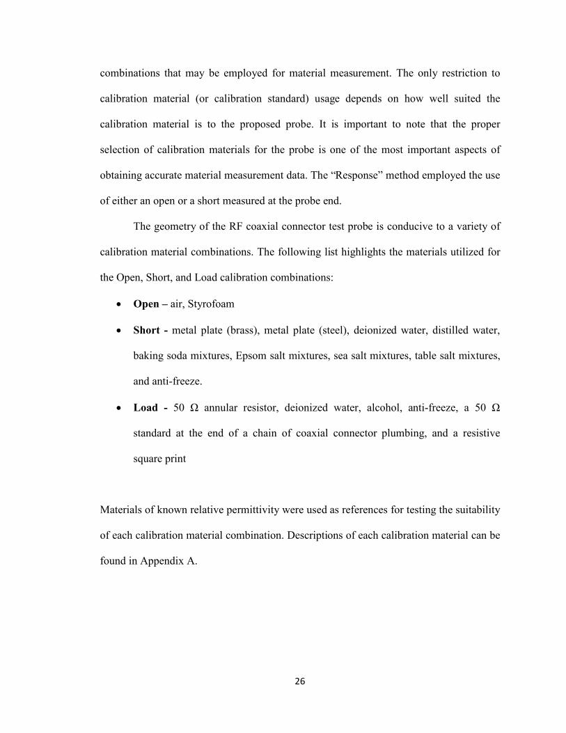
combinations that may be employed for material measurement. The only restriction to
calibration material (or calibration standard) usage depends on how well suited the
calibration material is to the proposed probe. It is important to note that the proper
selection of calibration materials for the probe is one of the most important aspects of
obtaining accurate material measurement data. The “Response” method employed the use
of either an open or a short measured at the probe end.
The geometry of the RF coaxial connector test probe is conducive to a variety of
calibration material combinations. The following list highlights the materials utilized for
the Open, Short, and Load calibration combinations:
• Open – air, Styrofoam
• Short - metal plate (brass), metal plate (steel), deionized water, distilled water,
baking soda mixtures, Epsom salt mixtures, sea salt mixtures, table salt mixtures,
and anti-freeze.
• Load - 50 Ω annular resistor, deionized water, alcohol, anti-freeze, a 50 Ω
standard at the end of a chain of coaxial connector plumbing, and a resistive
square print
Materials of known relative permittivity were used as references for testing the suitability
of each calibration material combination. Descriptions of each calibration material can be
found in Appendix A.

27
4.1.5 Measured Results from RF Coaxial Connector Test Probe
Two materials of known relative complex permittivity were used to verify the
measurement capability of the RF coaxial connector test probe at 0.55 to 1.8 GHz:
Polyethylene (Tivar) with an εr value around 2.25 - j0.0007 [16] other literature suggests
an εr’ of 2.3 [17] and Polycarbonate with an εr value around 2.85 - j0.003, found in [17]
from the EM Properties of Materials Project at NIST Boulder other literature suggests
εr’ of 2.9.
A Teflon sample, with an εr value of 2.1 - j0.0003, in [16], was used as the
reference material for these measurements. Eight separate calibration and measurement
data sets were taken for each calibration material combination. Table 4.2 shows the
complex permittivity mean value for each corresponding “Full-S11” calibration material
combination. Table 4.3 shows the complex permittivity mean value for each
corresponding “Response” calibration.

28
#
Full S11 - Calibration Material
Combinations
PE Polycarbonate
ε'r
2.3
(Stnd. Dev.)
ε''r 0.0007
(Stnd. Dev.)
ε'r
2.9
(Stnd. Dev.)
ε''r 0.0050
(Stnd. Dev.) Open Short Load
1 Air Metal
(brass)
(a) 50 Ω Annular
Resistor (AR)
2.310
(0.0072)
-0.0530
(0.1637)
2.704
(0.0237)
-0.2985
(0.1778)
(b) Anti-freeze 2.302
(0.0425)
-0.8761
(0.2444)
2.606
(0.0184)
-1.820
(0.4915)
2 Air Metal
(steel)
(a) 50 Ω AR 2.317
(0.0092)
-0.0730
(0.1587)
2.753
(0.0121)
-0.3117
(0.0829)
(b) Anti-freeze 2.305
(0.0094)
-1.105
(0.2811)
2.643
(0.0305)
-2.122
(0.5782)
(c) Alcohol
(90%)
2.359
(0.0114)
-2.159
(0.4852)
2.890
(0.0273)
-3.081
(0.7190)
(d) Deionized
water
2.112
(0.0064)
-0.9351
(0.3694)
2.124
(0.0196)
-1.388
(0.5360)
(e) 50 Ω
(plumbing)
2.333
(0.0045)
-0.1614
(0.0317)
2.745
(0.0080)
-0.2123
(0.0326)
3 Air Distilled
water
(a) 50 Ω AR 2.317
(0.0092)
0.3313
(0.3171)
2.703
(0.0315)
0.4145
(0.4349)
(b) Anti-freeze 2.247
(0.0060)
-0.6825
(0.1406)
2.675
(0.0261)
-1.315
(0.2630)
4 Air Deionized
(DI) water
(a) 50 Ω AR 2.323
(0.0120)
0.3305
(0.3200)
2.734
(0.0351)
0.4293
(0.4503)
(b) Anti-freeze 2.274
(0.0087)
-0.6510
(0.1331)
2.692
(0.0287)
-1.385
(0.2784)
(c) Alcohol
(90%)
2.354
(0.0113)
-1.783
(0.3453)
2.900
(0.0196)
-2.613
(0.5225)
5 Styro
foam
Metal
(steel)
(a) 50 Ω AR 2.317
(0.0055)
-0.1639
(0.1331)
2.737
(0.0137)
-0.3060
(0.0807)
(e) 50 Ω Standard
(plumbing)
2.345
(0.0059)
-0.1197
(0.0232)
2.662
(0.0064)
-0.1699
(0.0258)
(f) Square
Resistor
2.244
(0.0121)
-0.1158
(0.0576)
2.508
(0.0336)
-0.1722
(0.0786)
6 Styro
foam
Short Stnd.
(plumbing) (a)
50 Ω Stand.
(plumbing)
2.352
(0.0075)
-0.0832
(0.0197)
2.777
(0.0079)
-0.1341
(0.0214)
Table 4.2 Relative Permittivity Value for Full S11 Calibration Material Combo (test probe)

29
It can be seen from Table 4.2 that when using the 50-Ω annular resistor as the load
standard, the best calibration material combinations are #’s 2(a) and 4(a). This load
standard appears to be the best all around load that can be used for the RF coaxial
connector probe. In contrast, the 50 Ω commercial standard connected at the end of a
chain of coaxial connector plumbing works best when combined with the short standard
connected at the end of a chain of coaxial connector plumbing. This can be attributed to
accuracy of the pre-calibrated manufactured standards. Also, when using anti-freeze as
the load standard, the best calibration material combinations are #’s 3(b) and 4(b). It is
expected that the measured values, when using anti-freeze as a load, exhibit error because
anti-freeze is not well matched to the 50 Ω characteristic impedance load as it is used for.
It can also be noticed that when alcohol is used as the load standard, measurement values
are more precise when using a liquid for the short standard. Also, Styrofoam, as an open
standard, served well in the place of air. This is also expected because Styrofoam is
composed of mostly air with a εr’ of 1.03. The RF coaxial connector probe is a good
choice for obtaining room temperature measurements, but offers a few problems when
attempting to maintain a planar fit against measurement materials. It can be observed that
this one port measurement is not well suited for loss tangent measurements, unless
extremely precise calibration standards can be used.

30
# Response Calibration
PE Polycarbonate
ε'r
2.3
(Stnd. Dev.)
ε''r 0.0007
(Stnd. Dev.)
ε'r
2.9
(Stnd. Dev.)
ε''r 0.0050
(Stnd. Dev.)
7 Short
(a) Metal (brass) 2.383
(X)
0.9486
(X)
2.892
(X)
0.9062
(X)
(b) Metal (steel) 2.372
(X)
-0.1808
(X)
2.837
(X)
-0.2245
(X)
8 Open
(a) Air 2.347
(0.0090)
-0.0115
(0.0283)
2.788
(0.0166)
-0.0378
(0.0353)
(b) Styrofoam 2.332
(0.0114)
0.0085
(0.0318)
2.778
(0.0157)
-0.0155
(0.0364)
(X) – Standard deviation values are unusable due to abnormalities (Figure 4.7)
Table 4.3 shows that the “Open” Response calibration appears to more closely resemble
the data obtained from the three term “Full-S11” calibration. The “Open” Response
calibration displays a relatively smooth output while the “Short” Response calibration
exhibits inaccuracies at certain frequencies which make discovering the material’s actual
value difficult. For the “Short” Response Calibration measurements, the relative complex
permittivity median values were used due to the measurements exhibiting multiple
abnormalities at multiple frequencies. These abnormalities compromise the standard
deviation values as shown with Response calibration #7a, the measured value of
Polycarbonate using the “Short” Response Calibration with brass (Figure 4.7). The
abnormalities are assumed to be from the use of Response calibration materials that do
not closely resemble the electromagnetic properties of the tested materials. The
resemblance of calibration and tested materials during response calibration measurements
are important because the Response measurement only has a one-term error model to
Table 4.3 Relative Permittivity Value for Response Calibration (test probe)

31
Re
lati
ve
(Hz)
approximate with. For example, the reflection properties of air and Styrofoam resemble
an open standard, while metal and water resemble a short standard.
4.1.6 Repeatability of Measurement Procedure
To study the repeatability of the general measurement procedure described in
Chapter 4.1.3, the seven different room temperature Polyethylene measurements using
calibration combination #1(a) are depicted. In Figure 4.8 a plot of the relative permittivity
values (real vs. imaginary) of Tivar, extracted from the seven measurements taken, shows
consistency in the results.
0.4 0.6 0.8 1 1.2 1.4 1.6 1.8
x 109
-100
-50
0
50
100
150
200
250
300
Frequency
Permittivity
er'
er''
Abnormalities
Figure 4.7 Measured value of Polycarbonate using the
“Short” Response Calibration (brass)

32
4.1.7 Motivation of RF Coax Connector Test Probe Measurements on SS Probe
The results obtained from the RF coaxial connector test probe are used to validate
the results obtained from the stainless steel probe at room temperature. Since the
geometry of the stainless steel probe is not as user friendly as the RF Coaxial Connector
Test Probe geometry, it is anticipated that certain calibration combinations will not be
suitable for the stainless steel probe. Both the 50-Ω annular resistor and the 50-Ω from
the coaxial plumbing as the load standard should be well-matched to be used with the
stainless steel probe. Also, the alcohol standard should be well matched with the stainless
steel probe because it is a liquid and should maintain a good contact with the probe.
2.28 2.3 2.32 2.34 2.36 2.38 2.4-1.15
-1.14
-1.13
-1.12
-1.11
-1.1
-1.09
-1.08x 10
-4
Real Relative Permittivity
Imaginary Relative Permittivity
Variability of Procedure - RF Coaxial Test Probe
1
2
3
4
5
6
7
8
Figure 4.8 Relative Permittivity Value (Real vs Imaginary)
for Tivar of Eight Separate Measurements using the
Air, brass, 50 Ω AR Calibration Combination

33
Therefore, the calibration material combinations # 2(a), 2(c), 2(e), 4(c), 7, and 8 will be
used to evaluate the room temperature performance of the stainless steel probe.
4.2 Stainless Steel Probe
The stainless steel probe was made from a stainless steel pipe and a stainless steel
cylindrical rod connected to a RF NMale Clamp Type Connector. The stainless steel probe
assembly was based on the design restrictions and measurement results obtained from the
RF coaxial connector test probe. The RF coaxial connector test probe provides a good
means for material characterization at room temperature, but lacks the capability of
providing an adequate means for material characterization at high temperatures- hence
the need for a stainless steel probe for high temperature measurements. The results
measured from the stainless steel probe at room temperature use the same calibration
material combinations as the RF coaxial connector test probe. The results and design
restrictions of the original stainless steel probe influenced the addition of a spring-loaded
mechanism to combat the difficulties associated with the original stainless steel probe.
4.2.1 Stainless Steel Probe for Elevated Temperature Measurements
The stainless steel probe is used for elevated temperature measurements because
it offers the user a means of quickly and easily obtaining material measurements at
elevated temperatures. Stainless steel parts are readily available, and stainless steel has a
low thermal conductivity, making it the preferred conductor material because it allows
the user to comfortably hold one end of the probe while the other end is immersed in a
heated environment.

34
4.2.2 Construction of Stainless Steel Probe
The construction of the stainless steel probe was based on the structure of the RF
coaxial connector test probe. A one foot long stainless steel pipe used as the outer
conductor and a stainless steel cylindrical rod used as the center conductor were
electrically connected to an N-Male Clamp Type Connector on one end. In order to
provide a snug fit inside the ferrule of the N-Male Clamp Type Connector, the tube was
machined down, and a stainless steel washer was soldered to the opposite end of the pipe
to provide a flange, which acts as an extended ground plane. The stainless steel rod was
also soldered to the center pin. Three Teflon washers were then placed approximately 3
inches apart inside the stainless steel tube to provide a center positioned center conductor
in reference to the outer conductor. After all parts formed a flanged open ended-coaxial
probe, the probe end was machined flat and polished using 400, 600, 1000, and 2000
grade sand paper. The finished stainless steel probe is shown below in Figure 4.9.
Figure 4.9 Stainless Steel Probe

35
4.2.3 Stainless Steel Probe Geometry
The properties of the stainless steel coaxial probe are determined by using the
same formulas of a coaxial cable at high frequencies, equation (4.1) - (4.3). The
characteristics are listed in Table 4.4 as follows:
4.2.4 Stainless Steel Probe Room Temperature Setup
The stainless steel probe room temperature measurement apparatus consists of a
Vector Network Analyzer (VNA), the stainless steel probe, the calibration standards, the
reference material, and the material under test (Figure 4.10).
The SMA test port of the HP 4396B VNA is connected to an open-ended stainless
steel coaxial probe. In order to extract proper measurements, the stainless steel probe
must be placed firmly against the desired test quantity. The shaft of this probe is
approximately one foot long, so the user has the option to use a gripping apparatus
(Figure 4.11) or manually hold the probe firmly at the probe tip (Figure 4.12).
Stainless Steel Probe Properties
b 1.011 cm
a 0.3962 cm
εr 1 (air)
Zo 56.15
Table 4.4 Stainless Steel Probe Properties

36
Figure 4.10 Measurement Materials for Stainless
Steel Probe at room temperature
Figure 4.12 Stainless Steel probe placed
against a material during extraction
Figure 4.11 Stainless Steel probe held
with gripper during extraction

37
4.2.5 Calibration of the Stainless Steel Probe
The calibration of the stainless steel probe was realized by the use of a three term
“Full-S11” calibration technique, identical to the calibration applied to the RF coaxial
connector test probe in Chapter 4.1.4. Descriptions of each calibration material can be
found in Appendix A.
4.2.6 Measured Results from Stainless Steel Probe
Tivar with an εr value of 2.3 - j0.0007, in [16], and Polycarbonate with an εr value
of 2.9 - j0.0003, in [17], were used to verify the measurement capability of the stainless
steel coaxial probe at 0.55 to 1.8 GHz. Teflon, with an εr value of 2.1 - j0.0003 [16], was
used as the reference material. Eight separate calibration and measurement data sets were
taken for each calibration material combination. Table 4.5 shows the complex
permittivity mean value for each corresponding “Full-S11” calibration material
combination.
# Full S11 - Calibration Material
Combinations
PE Polycarbonate
ε'r
2.3
(Stnd. Dev.)
ε''r 0.0007
(Stnd. Dev.)
ε'r
2.9
(Stnd. Dev.)
ε''r 0.0050
(Stnd. Dev.)
2 Air Metal
(steel)
(a) 50 Ω AR 2.330
(0.0173)
-0.3407
(0.0686)
2.770
(0.0171)
-0.4748
(0.0958)
(c) Alcohol (90%) 2.331
(0.0290)
-1.097
(0.3568)
2.690
(0.0664)
-1.661
(0.5634)
(e) 50 Ω
(plumbing)
2.341
(0.0569)
-0.0464
(0.2813)
2.741
(0.0958)
-0.0613
(0.3808)
4 Air Deionized
(DI) water (c) Alcohol (90%)
Inconclusive, due to
center conductor movement
Table 4.5 Relative Permittivity Value for Calibration Material Combinations (SS probe)

38
It can be seen that only four calibration material combinations were taken using the
stainless steel probe. This was due to the difficulty presented in obtaining quality
measurements with the stainless steel probe. The probe offers a challenge in maintaining
a good planar fit to the material under test which limits the calibration usage. Even with
the use of liquid calibration combinations, this probe made measurement extraction very
difficult. The calibration material combination # 2(a) proved to be the best combination
to use for the stainless steel probe. Calibration material combination # 4(c) appeared to be
a good fit for this probe, but the data was unusable due to the erroneous center conductor
movement of the stainless steel probe. This data confirms the need for a better built
probe. The next logical progression is to find another method to test the validity of
stainless steel probe.
4.2.7 Motivation of Stainless Steel Probe Measurements on Spring-loaded Stainless
Steel Probe
The stainless steel probe presented the challenges of (1) maintaining a level
contact plane between the center and outer conductor, (2) maintaining intimate contact
among center conductor, outer conductor, and material under test, and (3) making an
allowance for the center conductor altering its initial position after coming in contact with
a material. These problems proved to amplify measurement difficultly which encouraged
the addition of a spring-loaded mechanism to be added to the center conductor.

39
4.3 Spring-loaded Stainless Steel Probe
The spring-loaded stainless steel coaxial probe was an enhancement to the
original stainless steel probe, with the major difference lying in a spring being inserted in
between the center pin and the stainless steel rod used for the center conductor. The
original stainless steel coaxial probe offered both a measurement difficulty and a
challenge in assuring both the center and outer conductor maintained an intimate contact
with the material under test. This probe also uses the same calibration material
combinations as the two preceding coaxial probes for obtaining room temperature
measurements. It is eventually used to obtain elevated temperature measurements.
4.3.1 Construction of Spring-loaded Stainless Steel Coaxial Probe
The construction of the spring-loaded
stainless steel coaxial probe was motivated by the
design restrictions associated with the original
stainless steel probe. A stainless steel pipe used as the
outer conductor and a stainless steel cylindrical rod
used as the center conductor were electrically
connected to an N-Male Clamp Type Connector on
one end. In order to provide a snug fit inside the
ferrule of the N-Male Clamp Type Connector, the
tube was machined down and silver-filled epoxy was
used to help provide a good electrical connection. A
stainless steel washer was soldiered to the opposite
Figure 4.13 Makeup of Spring-loaded
Stainless Steel Probe (modified
from [18])
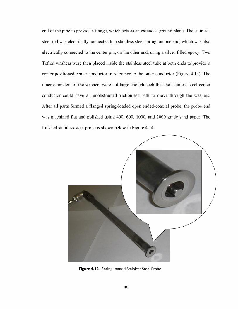
40
end of the pipe to provide a flange, which acts as an extended ground plane. The stainless
steel rod was electrically connected to a stainless steel spring, on one end, which was also
electrically connected to the center pin, on the other end, using a silver-filled epoxy. Two
Teflon washers were then placed inside the stainless steel tube at both ends to provide a
center positioned center conductor in reference to the outer conductor (Figure 4.13). The
inner diameters of the washers were cut large enough such that the stainless steel center
conductor could have an unobstructed-frictionless path to move through the washers.
After all parts formed a flanged spring-loaded open ended-coaxial probe, the probe end
was machined flat and polished using 400, 600, 1000, and 2000 grade sand paper. The
finished stainless steel probe is shown below in Figure 4.14.
Figure 4.14 Spring-loaded Stainless Steel Probe

41
4.3.2 Spring-loaded Stainless Steel Coaxial Probe Geometry
The properties of the spring-loaded stainless steel coaxial probe are determined by
using the same formulas of a coaxial cable at high frequencies, equation (4.1) - (4.3). The
characteristics are listed in Table 4.6 as follows:
4.3.3 Spring-loaded Stainless Steel Probe Room Temperature Setup
The spring-loaded stainless steel probe room temperature measurement set-up is
identical to the measurement set-up of the stainless steel probe described in Chapter
4.2.4.
4.3.4 Calibration of the Spring-loaded Stainless Steel Probe
The calibration of the spring-loaded stainless steel probe was realized by the use
of either a three term “Full-S11” calibration technique or a one term “Response”
calibration, identical to the calibration applied to the RF coaxial connector test probe in
Chapter 4.1.4. The only restriction to the exact type of calibration combination that may
be used is that the center conductor must be compressed. Descriptions of each calibration
material can be found in Appendix A.
Spring-loaded SS Probe Properties
b 1.011 cm
a 0.3962 cm
εrp 1 (air)
Zo 56.15
Table 4.6 Spring-loaded Stainless Steel Probe Properties
42
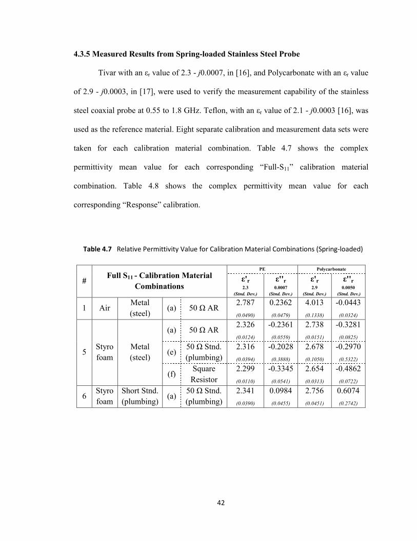
4.3.5 Measured Results from Spring-loaded Stainless Steel Probe
Tivar with an εr value of 2.3 - j0.0007, in [16], and Polycarbonate with an εr value
of 2.9 - j0.0003, in [17], were used to verify the measurement capability of the stainless
steel coaxial probe at 0.55 to 1.8 GHz. Teflon, with an εr value of 2.1 - j0.0003 [16], was
used as the reference material. Eight separate calibration and measurement data sets were
taken for each calibration material combination. Table 4.7 shows the complex
permittivity mean value for each corresponding “Full-S11” calibration material
combination. Table 4.8 shows the complex permittivity mean value for each
corresponding “Response” calibration.
# Full S11 - Calibration Material
Combinations
PE Polycarbonate
ε'r
2.3
(Stnd. Dev.)
ε''r 0.0007
(Stnd. Dev.)
ε'r
2.9
(Stnd. Dev.)
ε''r 0.0050
(Stnd. Dev.)
1 Air Metal
(steel) (a) 50 Ω AR
2.787
(0.0490)
0.2362
(0.0479)
4.013
(0.1338)
-0.0443
(0.0324)
5 Styro
foam
Metal
(steel)
(a) 50 Ω AR 2.326
(0.0124)
-0.2361
(0.0559)
2.738
(0.0151)
-0.3281
(0.0825)
(e) 50 Ω Stnd.
(plumbing)
2.316
(0.0394)
-0.2028
(0.3888)
2.678
(0.1050)
-0.2970
(0.5322)
(f) Square
Resistor
2.299
(0.0110)
-0.3345
(0.0541)
2.654
(0.0313)
-0.4862
(0.0722)
6 Styro
foam
Short Stnd.
(plumbing) (a)
50 Ω Stnd.
(plumbing)
2.341
(0.0390)
0.0984
(0.0455)
2.756
(0.0451)
0.6074
(0.2742)
Table 4.7 Relative Permittivity Value for Calibration Material Combinations (Spring-loaded)

43
The 50 Ω annular resistor still proves to be the best option available for use as the “load”
calibration standard. Also, the 50 Ω commercial standard connected at the end of a chain
of coaxial connector plumbing works well with the short standard connected at the end of
a chain of coaxial connector plumbing. The use of air as the “open” calibration standard
is not practical for use with the spring-loaded stainless steel probe because the electrical
length and characteristic impedance both change when the spring is compressed versus
being extended. The square resistor in theory would offer the best “load” calibration fit to
this probe because of its large surface area, but the impedance mismatch is too high. If a
square resistor with the proper 50 Ω characteristic impedance is used, it is then expected
to have comparable results, if not better, than the 50 Ω annular resistor. The 50 Ω annular
resistor still offers the challenge of aligning the spring-loaded probe with the resistor’s
metal contacts.
# Response Calibration
PE Polycarbonate
ε'r
2.3
(Stnd. Dev.)
ε''r 0.0007
(Stnd. Dev.)
ε'r
2.9
(Stnd. Dev.)
ε''r 0.0050
(Stnd. Dev.)
7 Short
(a) Metal (brass) 2.065
(X)
-0.0494
(X)
2.001
(X)
-0.0449
(X)
(b) Metal (steel) 2.063
(X)
-0.0326
(X)
1.999
(X)
-0.0317
(X)
8 Open
(a) Air 2.745
(X)
0.0715
(X)
3.916
(X)
0.0017
(X)
(b) Styrofoam 2.317
(0.0430)
-0.0107
(0.0250)
2.744
(0.1157)
-0.0572
(0.0359)
(X) – Standard deviation values are unusable due to abnormalities (Figure 4.15)
Table 4.8 Relative Permittivity Value for Response Calibration (Spring-loaded probe)

44
Re
lati
ve
(Hz)
It can be seen from Table 4.8 that the “Open” Response calibration appears to more
closely resemble the data obtained from the three term “Full-S11” calibration. The “Open”
Response calibration displays a relatively smooth output while the “Short” Response
calibration exhibits abnormalities at certain frequencies which make discovering the
material’s actual value difficult. The relative complex permittivity median values were
used for the “Short” Response Calibration measurements because these abnormalities
compromise the standard deviation values as shown with Response calibration #8a, the
measured value of Polyethylene using the “Open” Response Calibration with air (Figure
4.15). The “Air” calibration exhibits error because the spring-loaded probe’s center
conductor must be compressed in order to obtain accurate measurements as shown in
Chapter 4.3.5.
0.4 0.6 0.8 1 1.2 1.4 1.6 1.8
x 109
-35
-30
-25
-20
-15
-10
-5
0
5
10
15
Frequency
Permittivity
Permittivity Measurement - Method 1 (admittance)
er'
er''
Abnormalities
Figure 4.15 Measured value of Polyethylene using the
“Open” Response Calibration (air)

45
CHAPTER 5
COAXIAL PROBE FOR HIGH TEMPERATURE DIELECTRIC CHARACTERIZATIO
The spring-loaded stainless steel coaxial probe is used to extract material
properties at elevated temperatures. It offers an advantage over standard open-ended
coaxial probes by having a spring-loaded center conductor that forces an intimate contact
with the material under test. It has been noted that if this connection is compromised,
measurement results can be distorted by as high as 50% [19]. At elevated temperatures,
the probe and material interface should be of sound contact and should not require any
manual alterations, so as to not present any physical harm to the user.
5.1 Spring-loaded Stainless Steel Probe Elevated Temperature Setup
The spring-loaded stainless steel probe elevated temperature measurement set-up
was done such that high temperature measurements could be taken safely and without
damaging expensive equipment. The spring-loaded stainless steel coaxial probe elevated
temperature measurement apparatus consists of a Vector Network Analyzer (VNA), a
variable heating system (furnace), the spring-loaded stainless steel probe, the calibration
standards, the reference material, and the material under test.

46
The SMA test port of the HP 4396B VNA is connected to an open-ended coaxial
probe. An aluminum stopper is placed around the spring-loaded stainless steel probe and
both are inserted inside overhead opening of furnace. A clamp is then placed around the
aluminum stopper to control the probe’s insertion distance (Figure 5.1). In order to
extract proper measurements, the spring-loaded stainless steel probe must be placed
firmly against the test sample surface. It is necessary to add a brick inside the furnace to
ensure the material under test is at an acceptable elevation for testing (Figure 5.2).
Figure 5.1 Stainless Steel probe high temperature
measurement setup

47
5.2 Calibration of the Spring-loaded Stainless Steel Probe for Elevated
Temperatures
The calibration of the spring-loaded stainless steel probe was realized by the use
of either a three term “Full-S11” calibration technique or a one term “Response”
calibration, identical to the calibration applied to the RF coaxial connector test probe in
Figure 5.2 Stainless Steel probe placed against a
material during high temperature testing

48
Chapter 4.1.4. The only restriction to the exact type of calibration combination that may
be used is that the center conductor must be compressed.
During the initial measurement stage, the probe was calibrated with the three term
“Full-S11” calibration technique Styrofoam, Short Stand. (plumbing), 50 Ω Stand.
(plumbing). The probe, material under test, and reference material were all calibrated at
room temperature. The Styrofoam, short commercial standard connected at the end of a
chain of coaxial connector plumbing, and 50 Ω commercial standard connected at the end
of a chain of coaxial connector plumbing calibration was chosen because of the high
repeatability of the manufactured calibration standards. For subsequent measurement
stages, the one term “Response” calibration Styrofoam was used. For this calibration,
the probe and material under test were at the measurement temperature, while reference
material was at room temperature [20]. The one term “Response” method served to be the
best possible calibration sequence for high temperatures because of the dangers
associated with the calibration materials not being favorable for high temperature
measurements. Descriptions of each calibration material can be found in Appendix A.
5.3 Measured Results from Spring-loaded Stainless Steel Probe for Elevated
Temperatures
Teflon, with an εr value of 2.1 - j0.0003 [16], and Tivar, with an εr value of 2.3 -
j0.0007, in [16], were used to verify the measurement capability of the spring-loaded
stainless steel coaxial probe for elevated temperature measurements at 0.55 to 1.8 GHz.
Teflon was used as the reference material. Table 5.1 shows the complex relative
permittivity mean value for a room temperature “Full-S11” calibration used to measure

49
the materials at each respective temperature. The Full-S11 measurements were performed
such that one room temperature calibration was performed, and the resulting
measurements were performed at elevated temperatures. Table 5.2 shows the complex
relative permittivity mean value for each corresponding “Response” calibration at the
respective measurement temperature. The Response measurements were implemented
such that a new calibration and measurement were performed at each respective
temperature.
Full-S11 Calibration
Styrofoam, Short Stnd. (plumbing), 50 Ω Stnd. (plumbing)
Temp. (°C) Teflon Polyethylene
(23) ε'r
2.1
(Stnd. Dev.)
ε''r 0.0003
(Stnd. Dev.)
ε'r
2.3
(Stnd. Dev.)
ε''r 0.0007
(Stnd. Dev.)
23 2.11
(0.0203)
0.0492
(0.0925)
2.341
(0.0477)
0.0984
(0.1398)
45 2.258
(0.0329)
0.0660
(0.1106)
2.496
(0.0435)
0.0957
(0.1405)
75 2.318
(0.0321)
0.0690
(0.1165)
2.513
(0.0530)
0.0908
(0.1433)
100 2.338
(0.0310)
0.0650
(0.1184)
2.504
(0.0586)
0.0806
(0.1428)
The results from the “Full-S11” calibration (Table 5.1) agree for the room temperature
measurements, but start to exhibit error at higher temperatures. This increased error is a
result of the “Full-S11” calibration method not taking the effects of thermal expansion of
the probe into account. Figure 5.3 and Figure 5.4 show a plot of the “Full-S11” calibration
measurements taken at elevated temperatures. The probe’s accuracy farther decreases as
Table 5.1 Relative Permittivity Value for Full-S11 Calibration (SL probe)

50
Re
lati
ve
(Hz)
the characteristic impedance of the probe moves farther from the nominal room
temperature impedance value.
The effects of the thermal expansion of the probe are not taken into account with
this implementation. Therefore, the implementation of this calibration method is not
suggested for obtaining accurate elevated temperature measurements.
Figure 5.3 Relative Permittivity Extraction of Tivar at four temperatures using the
Room Temperature Full S11 Calibration
0.6 0.8 1 1.2 1.4 1.6 1.8
x 109
-0.5
0
0.5
1
1.5
2
2.5
3
Frequency
Perm
ittivity
Permittivity Measurement (Full S11)- Tivar
23 deg
23 deg
45 deg
45 deg
45 deg
45 deg
45 deg
45 deg
23 deg
23 deg
45 deg
45 deg
70 deg
70 deg
100 deg
100 deg
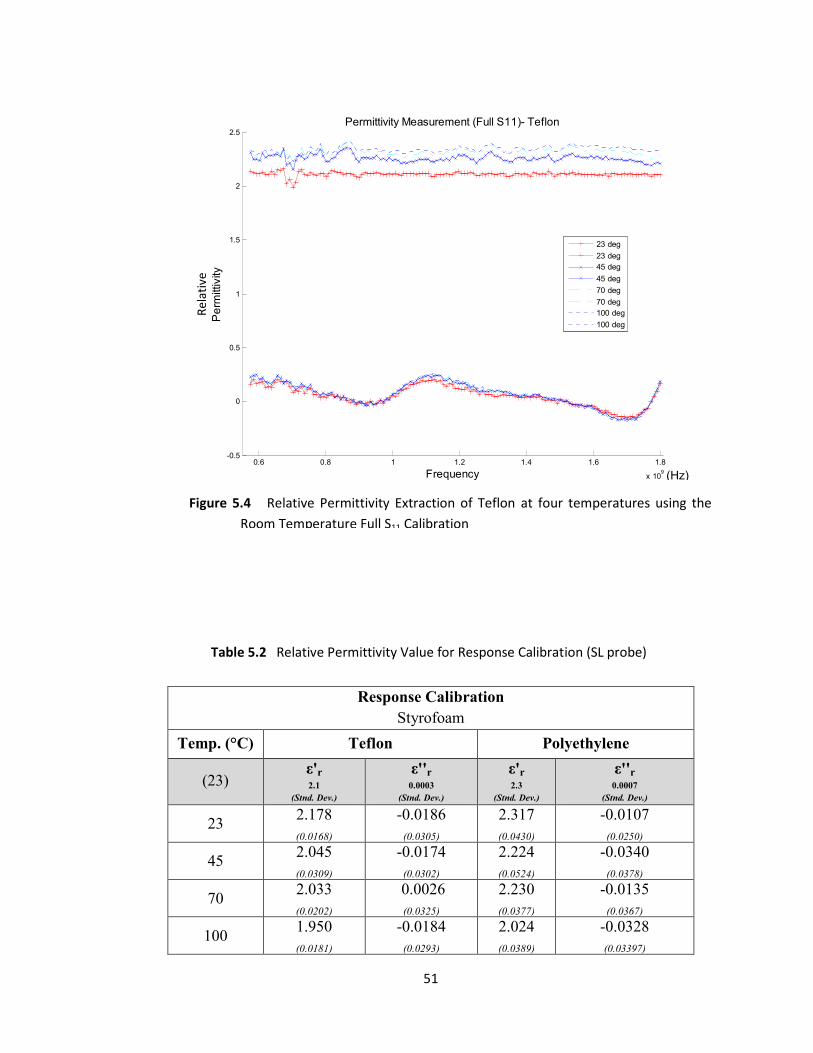
51
Re
lati
ve
23 deg
23 deg
45 deg
45 deg
70 deg
70 deg
100 deg
100 deg
23 deg
23 deg
45 deg
45 deg
70 deg
70 deg
100 deg
100 deg
23 deg
23 deg
45 deg
45 deg
70 deg
70 deg
100 deg
100 deg
(Hz)
Response Calibration
Styrofoam
Temp. (°C) Teflon Polyethylene
(23) ε'r
2.1
(Stnd. Dev.)
ε''r 0.0003
(Stnd. Dev.)
ε'r
2.3
(Stnd. Dev.)
ε''r 0.0007
(Stnd. Dev.)
23 2.178
(0.0168)
-0.0186
(0.0305)
2.317
(0.0430)
-0.0107
(0.0250)
45 2.045
(0.0309)
-0.0174
(0.0302)
2.224
(0.0524)
-0.0340
(0.0378)
70 2.033
(0.0202)
0.0026
(0.0325)
2.230
(0.0377)
-0.0135
(0.0367)
100 1.950
(0.0181)
-0.0184
(0.0293)
2.024
(0.0389)
-0.0328
(0.03397)
0.6 0.8 1 1.2 1.4 1.6 1.8
x 109
-0.5
0
0.5
1
1.5
2
2.5
Frequency
Perm
ittivity
Permittivity Measurement (Full S11)- Teflon
45 deg
45 deg
45 deg
45 deg
45 deg
45 deg
45 deg
45 deg
Table 5.2 Relative Permittivity Value for Response Calibration (SL probe)
Figure 5.4 Relative Permittivity Extraction of Teflon at four temperatures using the
Room Temperature Full S11 Calibration
23 deg
23 deg
45 deg
45 deg
70 deg
70 deg
100 deg
100 deg

52
0.6 0.8 1 1.2 1.4 1.6 1.8
x 109
-0.5
0
0.5
1
1.5
2
2.5
Frequency
Perm
ittivity
Permittivity Measurement (Response)- Tivar
23 deg
23 deg
45 deg
45 deg
70 deg
70 deg
100 deg
100 deg
Re
lati
ve
(Hz)
The results obtained from the “Response” calibration (Table 5.2) behave as expected. The
complex permittivity values decrease for both materials as temperature increases. The
effects of thermal expansion still play a role in the error exhibited by this method, but it is
expected that most of the error is from the calibration method. Figure 5.5 and Figure 5.6
show a plot of the “Response” calibration measurements taken at elevated temperatures.
As temperature increases, the relative permittivity values of both materials decrease.
The effects of the thermal expansion of the probe are taken into account with this
implementation, but the one term calibration method is not as accurate as a three term
calibration method. The implementation of this calibration method can be used to obtain
accurate elevated temperature measurements. It is important to note that the accuracy of
this extraction technique could further be increased if a three term calibration technique
could be used.
Figure 5.5 Relative Permittivity Extraction of Tivar at four
temperatures using the Response Calibration

53
Re
lati
ve
(Hz)
0.6 0.8 1 1.2 1.4 1.6 1.8
x 109
-0.5
0
0.5
1
1.5
2
2.5
Frequency
Perm
ittivity
Permittivity Measurement (Response)- Teflon
23 deg
23 deg
45 deg
45 deg
70 deg
70 deg
100 deg
100 deg
Figure 5.6 Relative Permittivity Extraction of Teflon at four
temperatures using the Response Calibration
54
CHAPTER 6
COCLUSIOS
6.1 Technique Summary
Three different open-ended coaxial probes were presented, and of these only one
was used to extract the complex permittivity of an unknown material at elevated
temperatures. The first probe or test probe is made from a highly polished- machined RF
coaxial connector. It was used as a bench mark for future measurements. The second
probe or stainless steel probe is made from stainless steel bars and a RF Clamp Type
Connector. This probe was the motivation behind creating the final probe. The final
probe or spring-loaded stainless steel probe is a variation of the original stainless steel
probe. It enhances the original probe setup with the addition of a spring-loaded
mechanism. It is the probe that is later used to test materials at elevated temperatures.
The probes are brought in contact with the tested material such that the fields at
the probe end fringe into the material. After this arrangement is formed, complex
permittivity is then extracted.
The lumped equivalent circuit capacitive model of the probe’s fields fringing into
a sample was used to extract the complex permittivity of materials using the open-ended
coaxial probe. This approach was selected because of the relative ease of implementation
as compared to other modeling techniques.

55
In order to increase accuracy of the solutions at elevated temperatures, the thermal
expansion of the coaxial probe must be taken into account. This was done by performing
a response calibration at each measurement temperature.
6.2 Future Work
This procedure served to give accurate material measurement results, but
precision can be further increased in both the room temperature and elevated temperature
measurements. The most immediate improvement that can be made lies in the equations
for extracting the complex permittivity. The lumped equivalent circuit model of the
probe’s fields fringing into a sample degrades at higher frequencies, and it has been noted
that measurements using a numerical computational method solution of the
electromagnetic field equations suitable for a coaxial line open to a dielectric sample are
generally more accurate (section 6.2.1). Also, further exploration into the calibration
standards utilized provides another source of improvement to this technique. Lastly, gold
plating the stainless steel probe will also enhance this technique.

56
6.2.1 umeric solution for an open-ended coaxial probe
Perhaps a more accurate modeling method, to relate the load admittance as a
function of the dielectric constant, is to implement a numerical computational method
solution of the electromagnetic field equations suitable for a coaxial line open to a
dielectric sample. The suggested approach for calculating a numerical solution of the
electromagnetic field equations suitable for an open-ended coaxial line was introduced by
D. K. Misra [23]. The model uses a quasi-static approximation which assumes that only
the dominant TEM mode propagates inside the coaxial line.
Misra formulated a stationary relationship for the aperture input admittance using
image theory and the boundary conditions of the tangential magnetic field equations as
shown in (2.8):
ρρφφπ
π
dddR
jkR
abk
kjY
b
a
b
arp
L '')exp(
'cos)/ln(
0
2
∫ ∫ ∫−
⋅=
(6.1)
where,
2
0ωεµ=k (6.2)
and
2
00 ωµεε rprpk = (6.3)
and
'cos'2'22 φρρρρ ++++====R (6.4)
where k is the wave number, krp is the wave number of the material inside the probe, and
ω is the angular frequency; a and b are the inner radius and the outer radius of the probe,

57
respectively; εrp is the relative permittivity of the dielectric material inside the probe and ε
is the total complex permittivity of unknown material under test (Figure 6.1).
The geometry of the probe end, as shown in Figure 6.2, shows the angles to and
distance between source point S and the field point F, respectively; R is the distance
between the source point and the field point; Φ is the angle between the field point and
the x-axis; Φ ' is the angle between the source point and the x-axis; ρ and ρ' are radial
coordinates of F and S, respectively, at the aperture of coaxial probe [24].
Figure 6.1 Open-ended coaxial probe in contact
with material of relative complex
permittivity, εr

58
Assuming the coaxial opening is electrically very small, equation (6.1) can be
approximated by the first few terms of the series expansion for the exponential term. The
characteristic admittance Y0 of the coaxial line can be obtained as follows:
(6.5)
Figure 6.2 The probe tip geometry defining
Equation (2.8). (Taken from An Open-ended
Coaxial Probe for Broad-band Permittivity
Measurement of Agricultural Products [24] )
0
0
0
ln
2
εεµ
π
rpa
bY
=

59
and
(6.6)
where
(6.7)
and
( ) ρρφφρρρρφπ
dddI
b
a
b
a
'''cos'2''cos0
22
3 ∫ ∫ ∫ += (6.8)
The second term of the series expansion goes to zero on integration over Φ’ and the
fourth term reduces to the last term of (6.6). Under this condition, (6.6) reduces to
(6.9)
I1 and I3 are integration constants which can be evaluated numerically for a given coaxial
line, independent of the tested medium characteristics, and are dependent only on the
physical dimensions of the aperture. A quadratic equation for the total complex
permittivity, ε, can be formulated using (6.9) for a measured admittance YL. Likewise,
the probe must be calibrated at the probe end in order to get accurate data [23].
2223
3
2
12 )/ln(122)]/[ln(
2
−+
−=
ab
abkIkI
abjYL
πωεωε
ρρφφρρρρ
φπ
dddI
b
a
b
a
'''cos'2'
'cos
022
1 ∫ ∫ ∫+
=
−≈ 3
2
12 2)]/[ln(
2I
kI
ab
jYL
ωε

60
6.2.2 Calibration Standards
The calibration standards are the main source of error, and the solution to this
problem simply lies in establishing more accurate calibration standards. The short circuit
can be better realized by using a conductive plastic polymer (i.e. Metal Rubber by
NanoSonic). This will not only have the conductive properties of a short, but also be
flexible enough to make sure an absolute short is obtained. The load calibration can be
enhanced by manufacturing a square resistor (in Appendix A.3) that has a characteristic
impedance of 50 Ω. I would suggest the use of a resistive paste with a resistivity of 1
Ω/. If the final screen printed resistor value is lower than 50 Ω, then this resistor can be
filed down to increase the surface resistance or the 1 Ω/ resistive paste can be combined
with a higher valued resistive paste until you reach the desired impedance (this will
produce a better resistor). Better calibrations will help both room temperature and
elevated temperature measurements.
For the elevated temperature set up, measurements calibrated with the probe and
material under test at the measurement temperature and the reference material at room
temperature will provide better elevated temperature measurements. In contrast, when the
probe, material under test, and reference material are all calibrated at room temperature,
measurements taken at elevated temperatures cause the system to drift. This system drift
or phase error is caused by the thermal expansion of the probe [20]. A simple calibration
at the desired temperature takes care of this problem. With better calibration standards for
elevated temperature measurements, a Full-S11 calibration can be taken at each
temperature, as opposed to a less accurate Response calibration. Also, another solution to
the thermal expansion problem with the probe would be to use a different conductive

61
material with a lower coefficient of thermal expansion (i.e. Kovar or a metalized
ceramic).
6.2.3 Gold Plated Probe
Gold plating the outside of the center conductor and the inside of the pipe to a
thickness of several skin depths would help with obtaining more accurate loss tangent
measurements. From different Wikipedia pages, the thermal conductivity of gold at 100
°C is 312.0 W/(m°C) and the electrical conductivity of gold is 44.64 x 10⁶ S/m (Table
6.1). Likewise, the thermal conductivity of stainless steel (316) at 100 °C is 16.20
W/(m°C) and the electrical conductivity of stainless steel (316) is 1.351 x 10⁶ S/m (Table
6.1). This means that gold is 33 times more electrically conductive than stainless steel,
making it the better conductor material to use for the probe. However, Table 6.1 also
shows that gold is 19 times more thermally conductive than stainless steel.
Fortunately, since gold is such a good electrical conductor, it offers a good compromise
even with the increased thermal conductance because the cross-sectional area over which
it will conduct heat is very small. Given this small cross-sectional area, my calculations
(Table 6.2) revealed a negligible amount of heat conducted by the gold.
Thermal Conductivity@ 100°C
W/(m°C)
Electrical Conductivity
S/m
Gold 312.0 44.64 x 10⁶
Stainless Steel 16.20 1.351 x 10⁶
Table 6.1 Thermal and Electrical Conductivities of Gold and Stainless
62
The skin depth, δ, is equal to
cfµσπδ 1= (6.10)
where f is the frequency, µ is the permeability, and σc is the conductivity of the metal.
When δ is small compared to the radius of the conductor, the AC resistance of the
conductor is about equal to the DC resistance of a conductor with a cross-sectional area,
A, equal to 2π·r·δ, where r is the radius of the conductor [25]. The total skin effect
resistance [26], in (6.11), is equal to the series combination of the inner conductor
resistance Rδa and the outer conductor resistance Rδb.
δσπδδδc
baba
LRRR
111
2
+=+=
(6.11)
where
δπσδa
LR
c
a2
1=
(6.12)
and
δπσδb
LR
c
b2
1=
(6.13)
where L is the length of the coaxial line, a is the radius of the inner conductor, and b is
the radius of the outer conductor.

63
The skin effect resistance [26] per unit length is equal to
c
f
baL
RR
σ
µπ
πδ
δ
+==11
2
1'
(6.14)
Therefore, the skin effect conductance per unit length is equal to
2
1
11
211'
L
ba
LRG c ⋅
+
⋅=⋅=
δσπ
δδ
(6.15)
and the total skin effect conductance, in (6.16), is equal to
L
ba
RG c 1
11
21⋅
+
⋅==
δσπ
δδ
(6.16)
This total skin effect conductance is also the heat conducted by the gold plating as shown
in Table 6.2.

64
Skin depth@ 1 GHz -410 x 9.0101 == cfµσπδ
[m]
Five skin depths thickness@ 1 GHz -410 x .05455 =⋅= δδ used
[m]
For δ << a and δ << b
Cross-sectional area
4-
-4
10 x 2.8612
10 x 1.1212
=⋅⋅=
=⋅⋅=
usedb
useda
bA
aA
δπ
δπ [m
2]
Inner conductor resistance@ L ≈ 12in = 0.3048m
8.7091
==ac
aA
LR
σδ [Ω]
Outer conductor resistance@ L ≈ 12in = 0.3048m
3.4141
==bc
bA
LR
σδ [Ω]
Total skin effect resistance
12.12=+= ba RRR δδδ [Ω]
Skin effect resistance per meter@ L ≈ 12in = 0.3048m
39.77' ==L
RR δ
δ [Ω/m]
Thermal conductance per meter@ L ≈ 12in = 0.3048m
0.2706 11
' =⋅=LR
Gδ
δ [S/m]
Heat conducted by gold plated probe
0.0825 1
==δ
δR
G [S]
(negligible)
Table 6.2 Calculations of Heat Conducted by Gold Plated probe
65
6.3 Conclusions
The open-ended coaxial probe method is a good approach when quick
permittivity measurements are desired. This method is most used with liquids, but with
the addition of the spring-loaded mechanism it serves as a good measurement system for
solids as well. The response calibration offers a quick calibration that is relatively
accurate. When measuring solids, an “Open” response calibration proves to work best,
likewise when measuring liquids the short “Short” response calibration appears to work
better. If elevated temperature measurements are desired, a three-term “Full-S11”
calibration at each measurement temperature will provide the most accurate results.
66
REFERECES
[1] H. Thomas, D. J. Elton, L. Riggs, S. Adanur, “Electronic Transmission and
Reinforcement Fabric,” National Textile Center Briefs, NTC Project: F05-Ae13,
Jun. 2007
[2] J. Baker-Jarvis, M. D. Janezic, J. H.Grosvenor, Jr., R. G. Geyer, “Transmission/
Reflection and Short-Circuit Line Methods for Measuring Permittivity and
Permeability,” Boulder, Co: NIST Technical Note 1355, 1992.
[3] Hewlett Packard, “HP Electronic Materials Measurement Seminar: A Broad
Spectrum of Solutions for Materials Characterization,” Hewlett Packard 5989-
1075E
[4] D. K. Ghodgaonkar, V. V. Varadan, “Free Space Measurement of Complex
Permittivity and Complex Permeability of Magnetic Materials at Microwave
Frequencies,” IEEE Trans. Instrum. Meas., Vol. 39, pp. 387–394, Apr. 1990.
[5] D. K. Ghodgaonkar, V. V. Varadan, V. K. Varadan, “A Freespace Method for
Measurement of Dielectric Constants and Loss Tangents at Microwave
Frequencies,” IEEE Trans. Instrum. Meas., Vol. 38. pp. 789-793, 1989.
[6] B. J. Wolfson, S. M. Wentworth, “Complex Permittivity and Permeability
Measurement Using A Rectangular Waveguide,” Microwave Opt. Techn. Lett.,
Vol. 27, No. 3, 180–182, Nov. 2000.
[7] C. A. Jones, “Permeability and Permittivity Measurements Using Stripline
Resonator Cavities: A Comparison,” IEEE Trans. Instrum. Meas., Vol. 48, pp.
843–848, Aug. 1999.

67
[8] Agilent Application Note, “Agilent Basics of Measuring the Dielectric Properties
of Materials,” Agilent Literature Number 5989-2589en, Jun. 2006
[9] T. T. Grove, M. F. Masters, R. E. Miers, “Determining Dielectric Constants
Using A Parallel Plate Capacitor,” Am. J. Phys., Vol. 73, No. 1, Jan. 2005
[10] M. N. O. Sadiku, Elements of Electromagnetics (2nd Ed). pp. 225-226. Saunders,
Fort Worth, 1994.
[11] Keqian Zhang, Dejie Li, Electromagnetic Theory for Microwaves and
Optoelectronics (2nd Ed). pp. 270-272. Springer-Verlag Berlin Heidelberg, 2008
[12] J. P. Grant, R. N. Clarke, G. T. Symm, N. M. Spyrou, “A Critical Study of The
Open‐Ended Coaxial‐Line Sensor Technique for RF and Microwave Complex
Permittivity Measurements,” J. Phys. E: Sci. Instrum., Vol. 22, 757‐770, 1989
[13] M. A. Stuchly, S. S. Stuchly, “Measurement of Radio Frequency Permittivity of
Biological Tissues with an Open‐Ended Coaxial Line: Part I - Part II,” IEEE
Tran. Microw. Theory Tech., Vol. 82, No. 1, 82‐92, 1982
[14] M. A. Stuchly, S. S. Stuchly, “Coaxial Line Reflection Methods for Measuring
Dielectric Properties of Biological Substances at Radio and Microwave
Frequencies-A Review,” IEEE Trans. Instrum. Meas., Vol. 29, No. 3, 176-183,
1980.
[15] D. Berube, F. M. Ghannouchi, P. Savard, “A Comparative Study of Four Open-
ended Coaxial Probe Models for Permittivity Measurements of Lossy
Dielectric/Biological Materials at Microwave Frequencies,” IEEE Tran. Microw.
Theory Tech., Vol. 44, No. 10, 1928-1934, 1996
[16] R. F. Harrington, Time-Harmonic Electromagnetic Fields, Mcgraw-Hill, inc.,
New York, pp. 72, 455, 1961
[17] B. Riddle, J. Baker-Jarvis, J. Krupka, “Complex Permittivity Measurements of
Common Plastics Over Variable Temperatures,” IEEE Tran. Microw. Theory
Tech., Vol. 51, No. 3, pp. 727–733, Mar. 2003.

68
[18] D. Gershon, J. P. Calame, Y. Carmel, T. M. Antonsen, Jr., “Open-Ended Coaxial
Probe for High-Temperature and Broadband Dielectric Measurements,” IEEE
Tran. Microw. Theory Tech., Vol. 47, No. 9, pp. 1640–1648, Sep. 1999.
[19] S. Bringhurst, M. F. Iskander, M. J. White, “Thin-Sample Measurements and
Error Analysis of High-Temperature Coaxial Dielectric Probes," IEEE Tran.
Microw. Theory Tech., Vol. 45, 12, pp.2073-2083, 1997.
[20] A. Lord, “Advanced RF Calibration Techniques,” Presentation, Cascade
Microtech Europe, Apr. 2002
[21] M. Sheffer, D. Mandler, “Why is Copper Locally Etched by Scanning
Electrochemical Microscopy?,” Journal of Electroanalytical Chemistry, Vol. 622,
pp. 115–120, 2008
[22] S. M. Wentworth, Applied Electromagnetics, Early Transmission Lines
Approach, Wiley, 2007
[23] D. K. Misra, “A Quasi-Static Analysis of Open-Ended Coaxial Lines,” IEEE
Tran. Microw. Theory Tech., Vol. 35, No.10, Oct. 1987
[24] N. I. Sheen, I. M. Woodhead, “An Open-Ended Coaxial Probe for Broad-Band
Permittivity Measurement of Agricultural Products,” J. Agric. Engineering. Res.,
Vol. 74, 193-202, 1999
[25] Koehler, Circuits and Networks, pp. 196, Excerpt from book found at
http://w8ji.com/skindepth.htm, Skindepth, Litz wire, Braided conductors, and
resistance, 2005
[26] S. M. Wentworth, Fundamentals of Electromagnetics with Engineering
Applications, Wiley, pp. 229, 2005

69
APPEDIX A
CALIBRATIO STADARDS OVERVIEW
Section A.1 addresses the calibration standards used for the “Open” calibration
standard. Section A.2 addresses the calibration standards used for the “Short” calibration
standard. Section A.3 addresses the calibration standards used for the “Load” calibration
standard. It is important to note that these are the calibration standards used in this
research, but data extraction is not limited to only these.
A.1 Open Calibration Standard
Air and Styrofoam were used as the “Open” calibration standard in this research.
Both were chosen because of their close resemblance to the relative permittivity of a
vacuum (εr = 1). For air the relative permittivity is equal to 1.00054. For Styrofoam
(Figure A.1) the relative permittivity is equal to 1.03.
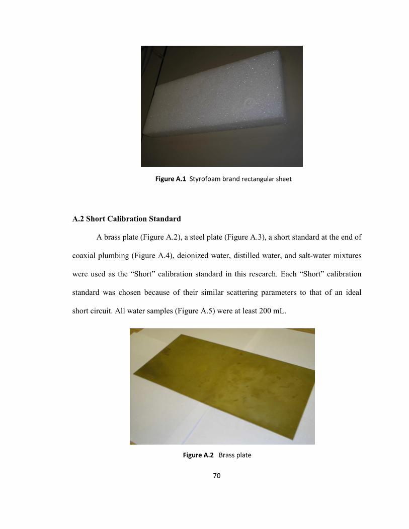
70
A.2 Short Calibration Standard
A brass plate (Figure A.2), a steel plate (Figure A.3), a short standard at the end of
coaxial plumbing (Figure A.4), deionized water, distilled water, and salt-water mixtures
were used as the “Short” calibration standard in this research. Each “Short” calibration
standard was chosen because of their similar scattering parameters to that of an ideal
short circuit. All water samples (Figure A.5) were at least 200 mL.
Figure A.1 Styrofoam brand rectangular sheet
Figure A.2 Brass plate
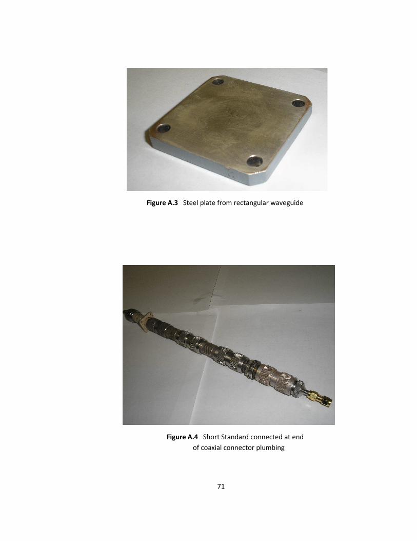
71
Figure A.4 Short Standard connected at end
of coaxial connector plumbing
Figure A.3 Steel plate from rectangular waveguide
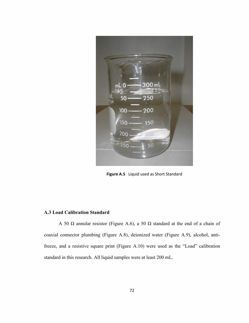
72
A.3 Load Calibration Standard
A 50 Ω annular resistor (Figure A.6), a 50 Ω standard at the end of a chain of
coaxial connector plumbing (Figure A.8), deionized water (Figure A.9), alcohol, anti-
freeze, and a resistive square print (Figure A.10) were used as the “Load” calibration
standard in this research. All liquid samples were at least 200 mL.
Figure A.5 Liquid used as Short Standard

73
The 50 Ω annular resistor (Figure A.5) ceramic sheet was created with multiple
50 Ω annular resistors such that all open-ended coaxial probes used in this work could fit
any one resistive element. The actual resistors were created through a commercial
fabrication process of screen printing, drying, and firing to apply the resistive material in
between the gold conductors. The theory behind the annular resistor is listed below:
Annular Resistor
The annular resistor is a ring or circular shaped resistive element surrounded by a
conductive material, where the inner and outer materials are very good conductors,
relative to the annular material in between them. The fabrication of the annular resistor
involved achieving both the correct resistive element to model a 50-Ω characteristic
Figure A.6 50 Ω Annular Resistor
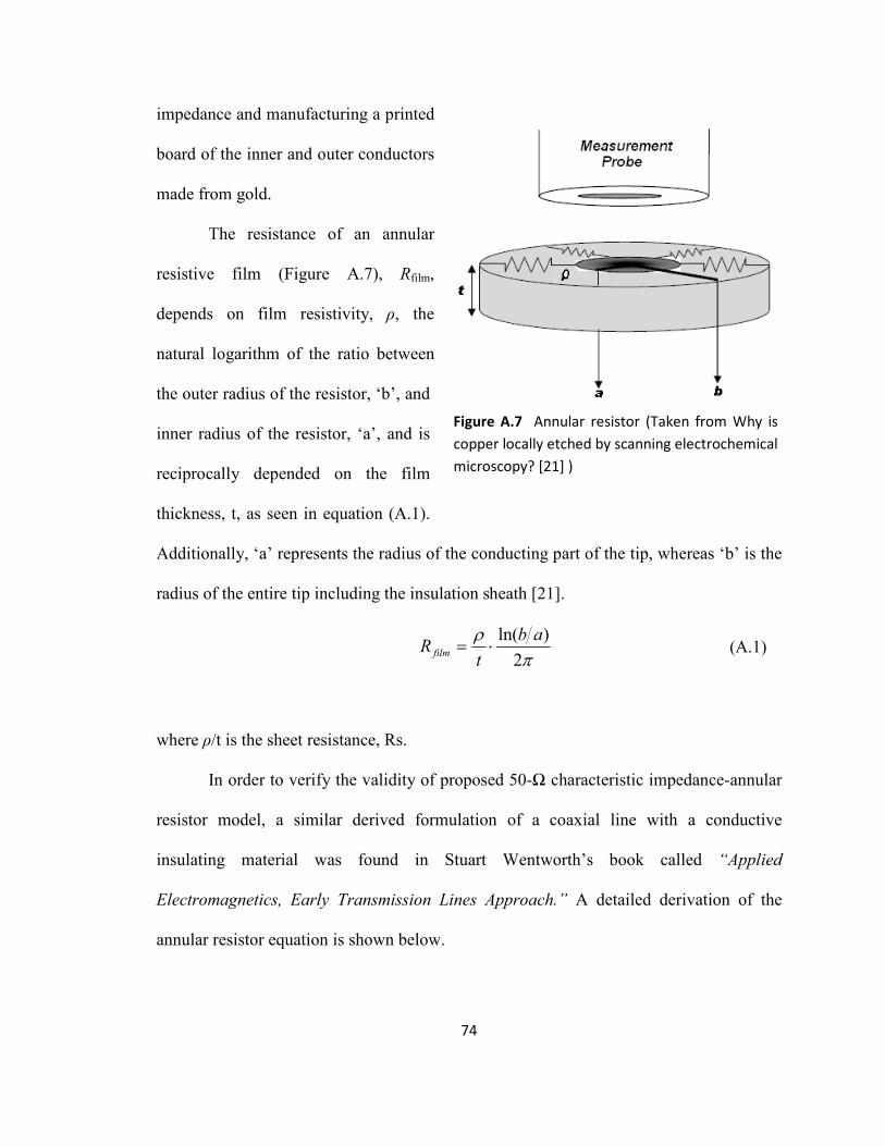
74
impedance and manufacturing a printed
board of the inner and outer conductors
made from gold.
The resistance of an annular
resistive film (Figure A.7), Rfilm,
depends on film resistivity, ρ, the
natural logarithm of the ratio between
the outer radius of the resistor, ‘b’, and
inner radius of the resistor, ‘a’, and is
reciprocally depended on the film
thickness, t, as seen in equation (A.1).
Additionally, ‘a’ represents the radius of the conducting part of the tip, whereas ‘b’ is the
radius of the entire tip including the insulation sheath [21].
πρ
2
)ln( ab
tR film ⋅=
(A.1)
where ρ/t is the sheet resistance, Rs.
In order to verify the validity of proposed 50-Ω characteristic impedance-annular
resistor model, a similar derived formulation of a coaxial line with a conductive
insulating material was found in Stuart Wentworth’s book called “Applied
Electromagnetics, Early Transmission Lines Approach.” A detailed derivation of the
annular resistor equation is shown below.
Figure A.7 Annular resistor (Taken from Why is
copper locally etched by scanning electrochemical
microscopy? [21] )
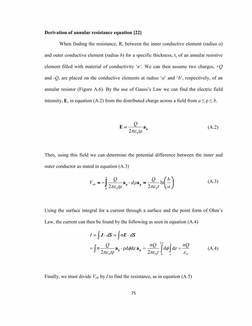
75
Derivation of annular resistance equation [22]
When finding the resistance, R, between the inner conductive element (radius a)
and outer conductive element (radius b) for a specific thickness, t, of an annular resistive
element filled with material of conductivity ‘σ’. We can then assume two charges, +Q
and -Q, are placed on the conductive elements at radius ‘a’ and ‘b’, respectively, of an
annular resistor (Figure A.6). By the use of Gauss’s Law we can find the electric field
intensity, E, in equation (A.2) from the distributed charge across a field from a ≤ ρ ≤ b.
ρaEρt
Q
02πε====
(A.2)
Then, using this field we can determine the potential difference between the inner and
outer conductor as stated in equation (A.3)
====⋅⋅⋅⋅−−−−==== ∫∫∫∫ a
b
t
Qρd
ρt
QV
a
b
ab ln22 00 πεπε ρρ aa (A.3)
Using the surface integral for a current through a surface and the point form of Ohm’s
Law, the current can then be found by the following as seen in equation (A.4)
0
2
000
σdzd
2
σ dzρd
ρ2σ
σ
εφ
πεφ
πε
πQ
t
Q
t
Q
ddI
t
o
==⋅=
⋅=⋅=
∫∫∫
∫∫
ρρ aa
SESJ
(A.4)
Finally, we must divide Vab by I to find the resistance, as in equation (A.5)

76
=a
bR film ln
πtσ2
1 (A.5)
where conductivity, σ, is the inverse of resistivity, ρ. Equation (5) can then be rewritten
as an equivalent expression to equation (1) by revising it in terms of the sheet resistance,
Rs (Ω/), as in equation (A.6).
=a
bRR S
film lnπ2
(A.6)
Fabrication
A MATLAB code was generated in order to calculate the correct sheet resistance.
After the desired sheet resistance was established, the next step was to obtain the
corresponding resistive pastes. The resistive paste samples were donated by Heraeus
Materials Technology, LLC.
The fabrication of the annular resistors involved getting both the correct resistive
element to model a 50-Ω impedance and manufacturing a screen printed board of the
inner and outer conductors made from gold. Michael Palmer performed most fabrication
work for the annular resistors.
The gold inner and outer conductors were printed first followed by the
commercial fabrication process of screen printing, drying, and firing to apply the resistive
material in between the gold conductors as depicted in Figure A.6. The fabricated annular
resistors had to be filed down with a Dremel tool due to the uncertainty of the thicknesses
applied during the screening printing process.
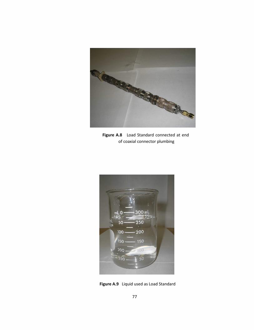
77
Figure A.8 Load Standard connected at end
of coaxial connector plumbing
Figure A.9 Liquid used as Load Standard

78
The resistive square print, referred to as the square resistor, (Figure A.10) was
created using the same fabrication process as the 50 Ω annular resistor. The square
resistor also went through a commercial fabrication process of screen printing, drying,
and firing to apply some resistive material onto a ceramic substrate. It was given the
trivial name “square resistor” for its square geometry. The only differences between the
square resistor and the 50 Ω annular resistors are that (1) the apparent area available for
the open-ended coaxial probes to contact is greater for the square resistor and (2) there
are no metal contacts constraining the probes placement. As a result of these differences,
the probe can be positioned anywhere on the resistive surface of the square resistor. Both
the greater available apparent area for contact and the decreased calibration difficulty
make the square resistor more ideal for the calibration process with the coaxial probes.
Figure A.10 Square Resistor (created using
same fabrication process as 50 Ω
Annular Resistor)

79
APPEDIX B
TECHIQUE DETAILS
The measurement process for the material characterization is relatively simple
using the open-ended coaxial probe method. This section will describe the room
temperature and elevated temperature calibration and measurement process. Also, the
calibration materials will be explored in greater detail.
B.1 Room Temperature Measurement Procedure
Below are the steps necessary for obtaining permittivity measurements at room
temperature using any open-ended coaxial probe.
1. Set up the VA
a. Format
i. More Admittance chart
b. BW/Avg.
i. Averaging ON
ii. Avg. Factor 16
c. Marker
i. This step just displays a marker on screen

80
d. Start
i. 100 kHz
e. Stop
i. 1.8 GHz
2. Perform automatic calibration (choose either “S11 1-port” or
“Response”)
a. Full S11 1-port
i. Cal
1. Correction ON
2. Calibrate Menu S11 1-port
ii. Pace probe flush against “Open” standard
1. Allow time for cable to stabilize
2. Press “Open”
a. For coax connector probe use Air or
Styrofoam
b. For spring-loaded probe use Styrofoam as
open
iii. Pace probe flush against “Short” standard
1. Allow time for cable to stabilize
2. Press “Short”
a. For coax connector probe use metal plate or
water

81
b. For spring-loaded probe use metal plate
iv. Pace probe flush against “Load” standard
1. Allow time for cable to stabilize
2. Press “Load”
v. Press “DONE: 1-PORT CAL”
b. Response
i. Cal
1. Correction ON
2. Calibrate Menu Response
3. Choose either “Open” or “Short”
ii. Pace probe flush against “Open” standard
1. Allow time for cable to stabilize
2. Press “Open”
a. For coax connector probe use Air or
Styrofoam
b. For spring-loaded probe use Styrofoam as
open
iii. Pace probe flush against “Short” standard
1. Allow time for cable to stabilize
2. Press “Short”
a. For coax connector probe use metal plate or
water
b. For spring-loaded probe use metal plate

82
iv. Press “DONE: RESPONSE”
3. Measure reference material (must use the different material for
reference then used for calibration)
a. Place probe flush against reference material
i. Allow time for cable to stabilize
b. Press SAVE
i. Data only Save ASCII
1. Disk must be loaded
4. Measure material under test
a. Place probe flush against material under test
i. Allow time for cable to stabilize
b. Press SAVE
i. Data only Save ASCII
1. Disk must be loaded
B.2 Elevated Temperature Measurement Procedure
Below are the steps necessary for obtaining permittivity measurements at elevated
temperatures using any open-ended coaxial probe.
1. Set up furnace (OTE: furnace overshoots desired temperature)
a. Insert stopper over probe and insert in top over furnace

83
b. Insert fire brinks and material under test to desired height of probe
tip
c. Turn furnace ON
2. Set up the VA
a. Format
i. More Admittance chart
b. BW/Avg.
i. Averaging ON
ii. Avg. Factor 16
c. Marker
i. This step just displays a marker on screen
d. Start
i. 100 kHz
e. Stop
i. 1.8 GHz
3. Perform automatic calibration (choose either “S11 1-port” or
“Response” or “Load” saved calibration)
a. Full S11 1-port
i. Cal
1. Correction ON
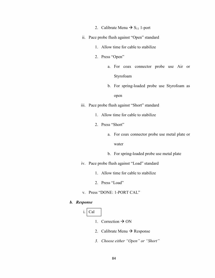
84
2. Calibrate Menu S11 1-port
ii. Pace probe flush against “Open” standard
1. Allow time for cable to stabilize
2. Press “Open”
a. For coax connector probe use Air or
Styrofoam
b. For spring-loaded probe use Styrofoam as
open
iii. Pace probe flush against “Short” standard
1. Allow time for cable to stabilize
2. Press “Short”
a. For coax connector probe use metal plate or
water
b. For spring-loaded probe use metal plate
iv. Pace probe flush against “Load” standard
1. Allow time for cable to stabilize
2. Press “Load”
v. Press “DONE: 1-PORT CAL”
b. Response
i. Cal
1. Correction ON
2. Calibrate Menu Response
3. Choose either “Open” or “Short”
85
ii. Pace probe flush against “Open” standard
1. Allow time for cable to stabilize
2. Press “Open”
a. For coax connector probe use Air or
Styrofoam
b. For spring-loaded probe use Styrofoam as
open
iii. Pace probe flush against “Short” standard
1. Allow time for cable to stabilize
2. Press “Short”
a. For coax connector probe use metal plate or
water
b. For spring-loaded probe use metal plate
iv. Press “DONE: RESPONSE”
c. Load saved Calibration
i. Load disk with saved calibration routine
ii. Recall
1. Choose file “____filename____”
4. Measure reference material (must use the different material for
reference then used for calibration)
a. Place probe flush against reference material
i. Allow time for cable to stabilize
b. Press SAVE

86
i. Data only Save ASCII
1. Disk must be loaded
5. Measure material under test
a. Place probe flush against material under test
i. Allow time for cable to stabilize
b. Press SAVE
i. Data only Save ASCII
1. Disk must be loaded

87
APPEDIX C
MATLAB CODE
C.1 Lump Equivalent Circuit Model Code
% This program reads Filename of text file of reference material (Filename_ref.txt),
% Filename of text file of material under test (Filename_MUT.txt), and Dielectric
% constant of reference material (K_ref) and solves for the Reflection Coefficient of the
% reference material (Gam_Ref), Reflection Coefficient of the material under test
% (Gam_Meas), the real relative permittivity (er_real) of the material under test, and the
% imaginary relative permittivity (er_imag) of the material under test
%-----------------------------------------------------
% If necessary program can also read the Reflection Coefficient of the Open
% calibration standard (GamCal_O), Reflection Coefficient of the Short
% calibration standard (GamCal_S), Reflection Coefficient of the Load
% calibration standard (GamCal_L) and apply a de-embedding algorithm
%-----------------------------------------------------
% INPUTS
% Filename_ref.txt - Filename of reference material
% Filename_MUT.txt - Filename of material under test
% K_ref - Dielectric constant of reference material (should be a
% material of known relative permittivity)
% number of rows to be used from loaded file (65 corresponds to 550 MHz
% and 201 corresponds to 1.8 GHz)
int = 65:201;
% load reference material data
load Filename_ref.txt % insert name of reference material file
refload= Filename_ref(:,1:3);

88
% load material under test data
load Filename_MUT.txt % insert name of material under test file
MUTload= Filename_MUT(:,1:3);
% frequency loaded from reference material
f = refload(int,1);
% radian frequency
w=2*pi.*f;
% Seperates reference material reflection coefficient into a real and
% imag component
S11_ref_r = refload(int,2); % real component of Reference Material S11
S11_ref_i = refload(int,3); % imaginary component of Reference Material S11
% calculate reflection coefficient of reference material
Gam_Ref = S11_ref_r - 1i*S11_ref_i;
%---------------------------------------
% Insert 1-port de-embedding HERE for "reference material" if necessary
%---------------------------------------
% Seperates material under test reflection coefficient into a real and
% imag component
S11_MUT_r = MUTload(int,2); % real component of Material under test S11
S11_MUT_i = MUTload(int,3); % imaginary component of Material under test S11
% calculate reflection coefficient of material under test
Gam_MUT = S11_MUT_r - 1i*S11_MUT_i;
%---------------------------------------
% Insert 1-port de-embedding HERE for "material under test" if necessary
%---------------------------------------
% characteristic impedance (50 ohms)
Zo = 50;

89
% characteristic admittance (0.2 ohms^-1)
Yo = 1/Zo;
% magnitude of reflection coefficient of reference material
Gamref_Mag = abs(Gam_Ref);
% Phase of reflection coefficient of reference material (in degrees)
Gamref_Phase =(180/pi).*angle(Gam_Ref);
% capacitance orginating from sample fringing field
Cs = (sind(Gamref_Phase).*Gamref_Mag.*(-2))./…
(w.*Zo.*K_ref.*(1+Gamref_Mag.*cosd(Gamref_Phase).*(2)+(Gamref_Mag).^2));
% capacitance orginating from probe fringing field
Cp =(-2.*Gamref_Mag.*sind(Gamref_Phase))./…
(w.*Zo.*(1+2.*Gamref_Mag.*cosd(Gamref_Phase)+(Gamref_Mag).^2)) - K_ref.*Cs;
% magnitude of reflection coefficient of material under
GamMUT_Mag = abs(Gam_MUT);
% phase of reflection coefficient of material under
GamMUT_Phase =(180/pi).*angle(Gam_MUT);
% calculate real relative permittivity (er) of the material under test
er_real= (2.*GamMUT_Mag.*sind(-GamMUT_Phase))./…
(w.*Cs.*Zo.*(GamMUT_Mag.^2 + 2.*GamMUT_Mag.*cosd(GamMUT_Phase)+1))…
- Cp./Cs;
% calculate imaginary relative permittivity (err) of the material under test
er_imag = (1-GamMUT_Mag.^2)./(w.*Cs.*Zo.*(GamMUT_Mag.^2 …
+ 2.*GamMUT_Mag.*cosd(GamMUT_Phase)+1));
C.1.a 1-Port De-embedding Algorithm
%% ------USE ONLY IF 1-PORT DE_EMBEDDING IS WANTED -------------
%% reflection coefficient of (open) calibration termination
% load Open_CAL.TXT
% dtc2 = Open_CAL(:,1:3);

90
% CAL_O_r = dtc2(int,2);
% CAL_O_i = dtc2(int,3);
%
%% reflection coefficient of (short) calibration termination
% load Short_CAL.TXT
% dtc1 = Short_CAL(:,1:3);
% CAL_S_r = dtc1(int,2);
% CAL_S_i = dtc1(int,3);
%
%% reflection coefficient of (load) calibration termination
% load Load_CAL.TXT
% dtc3 = Load_CAL(:,1:3);
% CAL_L_r = dtc3(int,2);
% CAL_L_i = dtc3(int,3);
%
%% CORRECTION METHOD
% MO = CAL_O_r -1i*CAL_O_i;
% MS = CAL_S_r -1i*CAL_S_i;
% ML = CAL_L_r -1i*CAL_L_i;
% SO = 1;
% SS = -1;
% SL = 0;
% K1 = ML-MS; %(approx. 1)
% K2 = MS-MO ; %(approx. -2)
% K3 = MO-ML ; %(approx. 1)
% K4= SL*SS*K1 ; %(approx. 0)
% K5= SO*SS*K2 ; %(approx. 2)
% K6= SL*SO*K3; %(approx. 0)
% K7=SO*K1 ; % (approx. 1)
% K8=SL*K2 ; % (approx. 0)
% K9=SS*K3; % (approx. -1)
% D1 = K4 + K5 + K6; % (approx. 2)
% a1= (MO.*K7 + ML.*K8 + MS.*K9)./D1; % (approx. 1)
% b1= (MO.*K4 + ML.*K5 +MS.*K6)./D1; % (approx. 0)
% c1 = (K7 + K8 + K9)./D1; %(approx. 0)
%
%% Correction for reference material
% GM1 = Gam_Ref;
% GA1 = (GM1 - b1)./(a1 - c1.*GM1);
% Gam_Ref = GA1;
%
%% Correction for material under test
% GM2 = Gam_MUT;
% GA2 = (GM2 - b1)./(a1 - c1.*GM2);
% Gam_MUT = GA1;
% ------------------------------------------------

91
C.2 umerical Method Extraction Code
The numerical method extraction algorithm presented did not accurately relate the
reflection coefficient of a material under test to the complex permittivity of that tested
material. This algorithm is only shown so that further work may be carried out on this
code.
% This program reads Filename of text file of reference material
% (Filename_ref.txt), Filename of text file of material under test
% (Filename_MUT.txt), Filename of text file of open calibration standard
% (Filename_OpenCAL.txt), Filename of text file of short calibration
% standard (Filename_ShortCAL.txt), Filename of text file of load
% calibration standard (Filename_LoadCAL.txt), the diameter of the inner
% conductor of the used probe (a), the diameter of the outer conductor of
% the used probe (b) and solves for the real relative permittivity
% (er_real) of the material under test, and the imaginary relative
% permittivity (er_imag) of the material under test
% INPUTS
% Filename_ref.txt - Filename of reference material
% Filename_MUT.txt - Filename of material under test
% Filename_OpenCAL.txt - Filename of text file of open calibration
% standard
% Filename_ShortCAL.txt - Filename of text file of short calibration
% standard
% Filename_LoadCAL.txt - Filename of text file of load calibration
% standard
% a - diameter of the inner conductor of the used probe (in inch)
% b - diameter of the outer conductor of the used probe (in inch)
% load reference material data
load Filename_ref.txt % insert name of reference material file
refload= Filename_ref(:,1:3);
% load reference material data
load Filename_MUT.txt %insert name of material under test file
MUTload= Filename_MUT(:,1:3);

92
% load reflection coefficient of (open) calibration termination
load Open_CAL.TXT
dtc2 = Open_CAL(:,1:3);
% load reflection coefficient of (short) calibration termination
load Short_CAL.TXT
dtc1 = Short_CAL(:,1:3);
% load reflection coefficient of (load) calibration termination
load Load_CAL.TXT
dtc3 = Load_CAL(:,1:3);
% frequency loaded from reference material
f = refload(int,1);
% radian frequency
w=2*pi.*f;
% Seperates reference material reflection coefficient into a real and
% imag component
S11_ref_r = refload(int,2); %real component of Reference Material S11
S11_ref_i = refload(int,3); %imaginary component of Reference Material S11
% calculate reflection coefficient of reference material
Gam_Ref = S11_ref_r - 1i*S11_ref_i;
% Seperates material under test reflection coefficient into a real and
% imag component
S11_MUT_r = MUTload(int,2); %real component of Material under test S11
S11_MUT_i = MUTload(int,3); %imaginary component of Material under test S11
% calculate reflection coefficient of material under test
Gam_MUT = S11_MUT_r - 1i*S11_MUT_i;
% Seperates open calibration reflection coefficient into a real and
% imag component
CAL_O_r = dtc2(int,2);
CAL_O_i = dtc2(int,3);

93
% calculate reflection coefficient of open calibration
GamCAL1_O = CAL_O_r -1i*CAL_O_i;
% Seperates short calibration reflection coefficient into a real and
% imag component
CAL_S_r = dtc1(int,2);
CAL_S_i = dtc1(int,3);
% calculate reflection coefficient of short calibration
GamCAL2_S = CAL_S_r -1i*CAL_S_i;
% Seperates load calibration reflection coefficient into a real and
% imag component
CAL_L_r = dtc3(int,2);
CAL_L_i = dtc3(int,3);
% calculate reflection coefficient of load calibration
GamCAL3_L = CAL_L_r -1i*CAL_L_i;
% speed of light
c=3e8;
% wavenumber
k = w./c;
% permittivity of free space
eps_0=8.854e-12;
% permeability of free space
mu_0=4*pi*10^-7;
eta=sqrt(mu_0/eps_0);
% freespace wavenumber
k0=w*sqrt(mu_0*eps_0);
% permittivty of dielctric inside probe
eps_c=2;
% characteristic admittance
Yo=2*pi/(log(b/a)*sqrt(mu_0/(eps_c*eps_0)));

94
% INTEGRATION
inTOcm =(1e-2/2.54); %converts from inches to centimeter
cmTOin =(2.54/1e-2); %converts from centimeter to inches
% outer diameter of probe
b= b*inTOcm;
% inner diameter of probe
a= a*inTOcm;
% integration functions
F = @(phiP,rhoP,rho) (cos(phiP))./(rho.^2 + rhoP.^2 - 2*rho.*rhoP.*cos(phiP)).^(1/2);
G = @(phiP,rhoP,rho) (cos(phiP)).*(rho.^2 + rhoP.^2 - 2*rho.*rhoP.*cos(phiP)).^(1/2);
% integration constants (triple integration)
I1 = triplequad(F,(.011),pi,a,b,a,b,[],@quadv);
I3 = triplequad(G,0,pi,a,b,a,b,[],@quadv);
%% CORRECTION METHOD
% % %Rho_m = is the measured reflection coefficient
% % %Gam_1 = the
% % %Gam_2 = the reflection coefficient of the standard 2 terminations used for
calibration
% % %Gam_3 = the reflection coefficient of the standard 3 terminations used for
calibration
% % %Rho_1 = the measured reflection coefficient corresponding to the calibration
termination 1
% % %Rho_2 = the measured reflection coefficient corresponding to the calibration
termination 2
% % %Rho_3 = the measured reflection coefficient corresponding to the calibration
termination 3
% reflection coefficient of short standard used for calibration
Gam_1 = -1; %short
% reflection coefficient of open standard used for calibration
Gam_2 = 1; %open
% reflection coefficient of load standard used for calibration
Gam_3 = 0; %load

95
S11 = (Gam_1.*Gam_2.*Rho_3.*(Rho_1-Rho_2)+ Gam_1.*Gam_3.*Rho_2.*(Rho_3-
Rho_1)+ Gam_2.*Gam_3.*Rho_1.*(Rho_2-Rho_3))./(Gam_1.*Gam_2.*(Rho_1-
Rho_2) … + Gam_1.*Gam_3.*(Rho_3-Rho_1)+ Gam_2.*Gam_3.*(Rho_2-Rho_3));
S22 = (Gam_1.*(Rho_2-S11)+Gam_2.*(S11-Rho_1))./(Gam_1.*Gam_2.*(Rho_2-
Rho_1));
S12nS21 = ((Rho_1-S11).*(1-S22.*Gam_1))./(Gam_1);
%true reflection coefficient
Gamma_true = (Rho_m-S11)./(S22.*Rho_m + S12nS21 - S11.*S22);
GamL= Gamma_true;
% constants for quadratic equation
const1= (1i.*w.*2)./((log(b/a))^2);
const2= const1.*(w.^2).*mu_0./2;
A=const2.*I3;
B=-const1.*I1;
C=(Yo.*(1-GamL)./(1+GamL));
% Correctionfactor (CF) is related to the reference material reflection
% coefficient
CF = ?????;
% Solved quadratic equation
X = (-B-sqrt(B.^2-4.*A.*C))./(2.*A)*(-CF);
% X = (-B-sqrt(B.^2-4.*A.*C))./(2.*A);
% the real relative permittivity (er_real) of the material under test
er_real = real(X);
% the imaginary relative permittivity (er_imag) of the material under test
er_imag = imag(X);