Coefficients of the Legendre and Fourier Series for theScattering Functions of Spherical Particles

J. V. Dave

Results of computations are presented to show the variations of coefficients of four different Legendreseries, one for each of the four scattering functions needed in describing directional dependence of theradiation scattered by a sphere. Values of the size parameter (x) covered for this purpose vary from0.01 to 100.0. Al adequate representation of the entire scattering function vs scattering angle curve isobtained after making use of about 2x + 10 terms of the series. It is shown that a section of a scatteringfunction vs scattering angle curve can be adequately represented by a fourier series with less than 2x +10 terms. The exact number of terms required for this purpose depends upoIi values of the size parame-ter and refractive index, as well as upon the values of the scattering angles defining the section understudy. Necessary expressions for coefficients of such fourier series are derived with the help of the addi-tion theorem of spherical harmonics.

1. Introduction

Currently, values of four scattering functions de-scribing the characteristics of electromagnetic radiationscattered by a sphere are usually computed from theexpressions for the same as derived by Mie.'- 5 How-ever, these scattering functions show strong variationswith scattering angle (0) when the radius (r) of thesphere is large compared to the wavelength (X) underinvestigation. In fact, for a sphere with size parameterx(= 2 7rr/X), a scattering function vs 0 curve showsabout x number of maxima and minima as 0 is variedfrom 0 to 1800. For several applications, it is desir-able to evaluate the field of the scattered radiation atabout lOx positions in the scattering angle. 7 Further-more, when one is interested in scattering character-istics of spherical polydispersions, it is necessary to com-pute these scattering functions for several hundredvalues of x for good reliability.8 9 Even with moderndigital computers, experience has shown that such com-putational tasks can be very tedious and time consum-ing.

Following Mie,' one first evaluates two complexquantities [Si(xm,0) and S2(xm,0)], where m is therefractive index of the material of the sphere with re-spect to its surroundings. Values of the four scatteringfunctions [1 2(x,n,0), AI,(xmO), S21(xm,0), and D2 1(xm,0) ] are then obtained by combining these quanti-ties.2 The expressions for S and 2 contain functions

The author is with the IBM Scientific Center, Palo Alto, Cali-fornia 94304.

Received 27 October 1969.

7rw(cosO) and T(COSO), which are expressible in termsof the first and second derivatives of the ordinaryLegendre functions, and hence produce the strong direc-tional dependence. Hartel 10 first suggested that theexpressions for these scattering functions could be sim-plified by the repeated use of recurrent relationshipsbetween the derivatives and products of Legendre func-tions."1 This would yield for each of these functions aseries whose terms are the ordinary Legendre poly-nomials weighted by coefficients depending upon m andx only. Chandrasekharl 2 showed that a solution of theequation of transfer in the nth approximation for ageneral phase function can be obtained by expressingthe phase function in the form of such Legendre series.Legendre series expressions for all four scattering func-tions were first derived by Sekera."3 Later, Chu andChurchill' 4 independently obtained similar expressionsfor the scalar phase function and published values ofthe coefficients of its Legendre series for some selectedvalues of x.'5 It was observed that such Legendrerepresentation of the scattering functions of a sphererequires about 2x + 10 number of terms, while thequantities Si and S2 are fully represented by about x +10 number of terms only. Fraser 6 used a modifiedLegendre series method for a limited study aimed atevaluating the characteristics of the radiation scatteredby spherical polydispersions. Further progress in thisdirection has been hampered because of the need toinclude a very large number of terms before meaningfulresults can be arrived at.

The purpose of this paper is twofold: (1) to discusssome of the computational results for the coefficients ofLegendre series representing scattering functions forspheres with size parameter up to 100; and (2) to showthat for cases where only a section of the entire scatter-

1888 APPLIED OPTICS / Vol. 9, No. 8 / August 1970

ing function vs 0 curve is required, equally reliablevalues can be obtained by including fewer terms. Suchcases are encountered very frequently during multiple-scattering calculations. 17

11. Coefficients of the Legendre Series

Necessary Expressions

As mentioned earlier, Sekera13 has expressed the fourscattering functions in the form of Legendre series. Inwhat follows, his final results are reproduced after someminor changes for conformity with current notation,and for adaptability to automatic computations. Thefirst scattering function appearing in Van de Hulst'stransformation matrix (Ref. 2, Sec. 5.14) is i112 (Xm0),

which is given by

a (k-1)/2 (-) 4(k -1)(k -) 2 ( ))a~kl)I(kl =(2k -1)(2k -3)(8)

and

bk-l) = k 2)2 bo(k-3). (9)

For k = 1, a(O) = 2 and bo(°) = 1. Then for m > k',am(k-) is obtained from the following recurrence rela-tionship:

a(k-1) (2m - k)(2m + k - 1) a_(k-1),- (2m + k)(2m - k + 1)

and for i > 0, b(k1-) is given by

b,(k-1) = (k - 2i + 1)(k + 2i - 2) bi 1 (k-1).(k - 2i)(k + 2i - 1)

(10)

(11)

M 2(xm0) = Z Lk(1)(xm)Pkl(cosO).k = 1

(1)

Similar expressions for the remaining three elements,viz., M(xm,0), S2 1(xm,0), and D21 (xmO), can be ob-tained after substituting j = 2, 3, and 4, respectively,in Lk(j)(xm).

The Legendre coefficients Lk(j)(x,m) are given byk'

LkC')(x,m) = (k - 0.5) E am(k'1) E bm=lk' i=O

X Re[Dp(x,m)Dq*(x,m)], (2)

k'Lk(')(x,m) = (k - 0.5) , am.(k-1) E b(k l)A

m=1k' i = O

X Re[Cp(x,m)Cq*(x,m)1, (3)

k'LkC')(x,m) = (0.5k - 0.25) E am(k-1) (k -1); k

m= k' i = O

X Re[Cp(x,m)D,*(x,m) + Cr*(x,m)D,(x,m)l,

and

For even values of k > 2, the quantities am(k-1) andb(k-1) are first computed using the following recurrencerelationships for a value of m = k' and i = 0, respec-tively:

(k 1 ) =4(k -1)(k -) (k 3)a=-)/ (2k - 1)(2k - 3) ack-42, (12)

and

(13)bW(k-') = (k - 1)(k - 3) bo('-')k(k - 2)

For k = 2, ao(l) = and boM1' = 2. Then for'm > k',am(k-) is obtained after making use of the following re-currence relationship:a,(") (2m -k + 1)(2m + k) k1

(4) (2m + k + 1)(2m - k + 2) -"-,

and for i > 0, b(k-1) is obtained from

(14)

Lk(4 )(x,m) = (0.5k - 0.25) s am(k-i) E bi (k l)Akm = k ' i = O

X Im[Cp(x,m)Dq*(x,m) - Cp*(x,m)Dq(x,rn)]. (5)

The superscript asterisk (*) represents the complexconjugate of the corresponding function. The symbolsRe ] and Im[ ] imply the real and imaginary part,respectively, of the complex quantity within the en-closed brackets.

((k - 1)/2 for odd k,k' = t (6)

L(k - 2)/2 for even k.

f1 for i = 0, odd k,Aik = 2 for i > 0, odd k, (7)

i2 for i > 0, even k.

The subscripts p and q are given by p = m - i + 1 andq = m + i + 1 + , where 3 = 0 for odd values of k,and 5 = 1 for even values of k.

For odd values of k > 1, the quantities am(k-) andbi(k1-) are first obtained after using the following recur-rence relationships for a value of m = k', and of i = 0,respectively:

b (k-l) (2i + k - 1)(2i - k) bil(k-l)(2; - k + 1)(2i + k)

(15)

Finally, the complex functions CQ(x,m) and Dk(xm)[where k here stands for p or q in Eqs. (2)-(5) ] are com-puted from the values of the complex Mie amplitudesan(x,m) and bn(x,m) (Refs. 4 and 7) by means of the fol-lowing formulas:

Ck(x,m) = (1/k)(2k - 1)(k - 1)b.,(x,m)

+ (2k - 1) E { [p-1 + (p + 1)-]ap(x,m)

- [(p + 1)-' + (p + 2)-']bp+(x,m)l, (16)

and

Dk(X,m) = (1/k)(2k - 1)(k - 1)ak_(x,m)

+ (2k - 1) E { [p-' + (p + 1'lbp(x,in)i = 1

- [(p + 1)-1 + (p + 2)-1]ap+&~,m)}, (17)

where for Eqs. (16) and (17), p = k + 2i - 2. Evi-dently, ao(x,m) = b(x,m) = 0.

August 1970 / Vol. 9, No. 8 / APPLIED OPTICS 1889

Variations of the Legendre Coefficientswith Size Parameter

The values of the Legendre coefficients L(x,m)were computed for several values of x and m = 1.342using an IBM System/360 Model 91 computer anddouble precision arithmetic. Starting with a value of xand m, the CPU time required for computations of allcoefficients for x = 10 and 100 was about 0.1 see and 16sec, respectively. Values of the scattering functions1112, M1, S21, and D21 as obtained from the use of Eq. (1),and from the values of Si(xm,0) and S2(xm,0), werefound to agree up to five significant figures for severaltest cases for which some manual checks were per-formed. In what follows, we shall refer to the normal-ized coefficients given by

Ak' (xm) = [4/Q. (x,rn)x'jLk i(x,?n), (18)

where Q,(x,m) is the so-called efficiency factor for scat-tering. 2

The values of the first five normalized coefficients forj = 1 and forx = 0.01, 0.1, and 1.0 are given in Table I.For x = 0.01 and 0.1, values of these coefficients cor-responding to k = 1 and 3 are exactly the same as thosepredicted by Rayleigh's law of scattering. As x in-creases from 0.1 to 1.0, values of these two coefficientsshow a small but significant increase. On the otherhand, values of the remaining three coefficients (k = 2,4, and 5) which vanish in the Rayleigh limit, show avery rapid increase with x. Similar trends were alsoseen in the values of these coefficients for j = 2 and 3,except that now the only nonvanishing coefficients inthe Rayleigh limit are A( 2)(x,m) and A2(3 )(x,m), witheach having a value of 1.5. For j = 4, the highestabsolute values of the normalized Legendre coefficientsare 4.3 X 10-13, 4.3 X 10-8, and 3.2 X 10-3 for x =0.01, 0.1, and 1.0, respectively. These variations implythat significant deviations in the polarization charac-teristics from the Rayleigh case become evident whenx - 0.1. However, even a sphere with size parameterof the order of unity would exhibit extremely weakelliptical polarization, if any.

Values of the first 35 normalized Legendre coefficientsfor j = 1 through 4 are presented in Table II for asphere with size parameter x 10 and m = 1.342.The main purpose of this table is to provide the readerwith at least one complete set of values which he canuse for independent checking of his computer pro-gram. Except for round-off errors, all the values areexpected to be correct up to five significant places. Itshould be added that scattering functions for variousvalues of 0 should be computed from values whichcarry all significant figures available inside the com-puter. From Table II, it can be seen that the series foreach of the scattering functions can be terminated afterabout 30 terms, i.e., the upper limit for summation inEq. (1) is not infinity but N, where N 2x + 10.

In Fig. 1, we have presented variations of the abso-lute values of the Legendre coefficients of the series forthe scattering function M 2(x,m,0) as a function of ,for three different values of x, viz., 20, 50, and 100.

Table I. Values of the First Five Normalized Coefficients ofLegendre Series for the Scattering Function

M 2 (xm,0); m = 1.342

k A.(1) (0.01, In) Ak0 (.1, m) Ak(l) (1.0, m)

1 5.0000 (-01)a 5.0000 (-1) 5.1269 (-1)2 4.3767(-05) 4.3749 (-3) 4.4557 (-1)3 1.0000 1.0000 1.03714 2.3029 (-05) 2.3012 (-3) 2.2534 (-1)5 1.2627 (-10) 1.2608 (-6) 2.1224 (-2)

a The number in the parenthesis represents the power of 10 bywhich the preceding number is to be multiplied, e.g., 5.0 (-01)= 5.0 X 10-'. If there is no parentheses after the number, thepower of 10 is equal to zero.

Only a few of the coefficients assume negative values,e.g., for x = 50, the coefficients A,(l)(x,m) are negativefor k = 104, 105, 106, and 110 only. For these threevalues of x, Al(')(x,m) is very close to unity, and againthe series can be terminated when N-. 2x + 10. Thecurves of A,(')(xm)I vs subscript k are fairly smoothexcept for n > 2x, where the slope is very steep. Forclarity of the diagrams, a few alternate values areomitted in the region where there is very little differ-ence between two successive values. The variations ofJA,(2)(Xm)I and Ak(3)(xm)j as functions of k were alsofound to show similar trends.

The variations in Ak(4) (x,m) as a function of k arevery erratic, and as such their graphical presentationposes some problem. Some of the possible confusion isavoided by plotting absolute values of these coefficientsvs k in two different sets; the upper curves in Figs. 2and 3 represent variations in Ak(4)(x,m)I vs k for evenvalues of k, while the lower curves are for odd values of k.In Fig. 2, results of computation are presented for x =

2 * *--------------------@: m 1.342

10'

X=20 x=50. x=100100

103

t 3 _ .40 80 120 160 200SUBSCRIPT IkI

Fig. 1. Variations of the absolute values of normalized coeffi-cients of the Legendre series for the scattering function M,(xm, 0)

as a function of subscript k of the coefficient.

1890 APPLIED OPTICS / Vol. 9, No. 8 / August 1970

Table II. Values of the Normalized Coefficients of the Legendre Series for Scattering Functions of a Sphere; x = 10.0, m = 1.342

k Ak()(xm) Ak(2)(x,m) Ak(')(x,m) Ak( 4)(x,m)

1 1.0645 9.3551 (-1) 9.0259 (-1) -1.0109 (-1)2 2.1853 1.9286 2.0843 4.4926(-2)3 2.7321 2.7926 2.6642 -9.0608 (-2)4 2.5467 2.4535 2.4983 2.9276(-2)5 2.2937 2.3913 2.3778 1.3266(-1)6 2.1454 2.2061 2.0681 4.6171 (-2)7 2.0520 2.0194 2.1048 2.9736(-l)8 2.1552 2.0738 2.0710 1.6766(-1)9 2.3562 2.1007 2.2183 2.9973(-1)

10 2.5434 2.3038 2.4925 2.8820(-1)11 2.9173 2.4815 2.6113 2.7102(-1)12 3.1462 2.7860 3.1150 3.5453(-1)13 3.4761 3.1150 3.2254 2.8577(-1)14 3.8971 3.5953 3.8084 3.1660(-1)15 3.9568 3.9086 4.0649 3.7816 (-1)16 4.4225 4.7123 4.4791 6.1476( -2)17 4.1765 4.5631 4.5421 2.5024(-1)18 3.8141 5.0155 4.5404 -3.7044 (-1)19 3.0307 4.0056 3.5374 -7.8945 (-1)20 2.2171 2.5007 2.4057 -8.7630 (-1)21 1.4823 1.3086 1.1182 -9.0760 (-1)22 3.4957 (-1) -1.2688 (-1) 1.0509 (-1) -5.4768 (-2)23 1.4843 (-1) 7.2065 (-2) 9.5872 (-2) -2.4685 (-2)24 4.5331 (-2) 2.0767 (-2) 2.9265 (-2) -7.0836 (-3)25 1.1477 (-2) 4.5711 (-3) 7.0955 (-3) -1.4658 (-3)26 2.5031 (-3) 8.4961 (-4) 1.4629 (-3) -2.4298 (-4)27 4.8173 (-4) 1.3824 (-4) 2.6389(-4) -3.3629 (-5)28 8.3323 (-5) 2.0143 (-5) 4.2478 (-5) -3.9757 (-6)29 1.3134 (-5) 2.6727 (-6) 6.1969 (-6) -4.0650 (-7)30 1.9069 (-6) 3.2724 (-7) 8.2970 (-7) -3.5526 (-8)31 2.5508(-7) 3.7323 (-8) 1.0310 (-7) -1.3215 (-9)32 3.0920 (-8) 3.7615 (-9) 1.1234 (-8) -1.1240 (-11)

33 3.4798 (-9) 3.5833 (- 10) 1.1529 (-9) -5.5487 (-14)34 3.5894(-10) 3.1542 (-11) 1.0902 (-10) 1.8598 (-15)35 3.3466 (-11) 2.5254 (-12) 9.3547 (-12) 6.5504 (- 17)

20 and 50, while those in Fig. 3 are for x = 100. Unlikethe values of the coefficients for the other three scatter-ing functions, several values of A,(4) (x,m) carry a nega-tive sign. It is interesting to note that the Legendrecoefficients for this fourth scattering function attaintheir highest values when k - 2x; it is not so for theother three cases (e.g., Fig. 1).

To determine the scattering properties of a unitvolume of spherical polydispersions, it is necessary tointegrate the unnormalized Legendre coefficients overthe size-distribution. For this purpose, it is desir-able to study, in some detail, variations of LjcM(xm) as a function of x. In Fig. 4, values of L,(J)(x,m)/x2 and Q8(x,m) are plotted as a function of size parame-ter in the range x = 10.00 (0.05) 15.00. Variations inQ8(x,m) as a function of x (lowermost curve) are identi-cal to those presented on a much more extensive scaleby Penndorf.' 8 A more detailed discussion of thesevariations can be found in Ref. 2 (Secs. 11.22, 13.42,and 17.26). It will suffice to state here that this curveshows a periodicity of about 0.8 in x superimposed overanother variation having much greater periodicity and

10 0

: O I21

0 4

I I I ."

0 40 80 120SUBSCRIPT (I

Fig. 2. Variations of the absolute values of normalized coeffi-cients of the Legendre series for the scattering function D21(x, M,0) as a function of subscript k of the coefficient. For clarity,coefficients with odd and even values of k are plotted separ-

ately.

August 1970 / Vol. 9, No. 7 / APPLIED OPTICS 1891

010 I

0

10

z>

-

0

0

0o

en

0.2 - - C 7T - fl

0., - 4r \--- 1, j , V.., 1.., ,.,.

-I I

iI

I- __X = I

� M = 1�10 �2 ___ __ -

I I 1 1 1 1 1 .

� k I

........................

-0.

El

_ w

I(S-1 _J-�P � '..,

j 'IV1.

16, � - it

116, 1 - I I I -

0 40 soSUBSCRIPT

120 160 200 12 13SIZE PARAMETER x

Fig. 5. Same as Fig. 4 but for k = 16.Fig. 3 Same as Fig. 2.

amplitude. The curves of the coefficient,,three scattering functions (j = 2 and ations similar to those for Q,,(xm) except t]values increase much more rapidly with sifor x > 12.5. The presence of some aWdisturbance is also noticeable on Li (3) (j

curve (dotted curve). The function LI'negative for all values of x of interest to cussion (topmost curve). The maxima animuch sharper compared with those fordiscussed above. Besides, one now obs(additional maxima and minima for 13.0Similar results for L(J)16(XM) IX2 correspondthrough 4 are presented in Fig. 5. For thEtering function D21(X^0), these coefficieipositive sign at several places.

3 for the first Values of LW26(xm) show about a four orders-of-3) show vari- magnitude increase as x is increased from 10 to 15.W now their Furthermore, for each of the four cases (j = throughze parameter 4), we find that some values of these functions are nega-itional minor tive. Therefore, in Figs. 6 and 7 we have plotted as a,,M)/X2 VS X function of x, absolute values of L(J)26(XM) on a(4) (x,?n)/X2 is semilogarithmic scale. The Legendre coefficients of theis in this dis- series for M2(XMO) (solid curve in Fig. 6 are positived. minima are and increase by about two orders of magnitude as xother cases increases from 10 to 11.5. A further small increase in x

-rves several results in a very rapid decrease. The values of L(')26

< x _< 15.0. (xm) at x = 11.90, 11.95, and 12.00 are negative. An-ling to j = I other small increase in x by 0.05 results in a change offourth scat- sign, and the function increases by three orders of mag-

ats exhibit a nitude as x is increased from 12.05 to 12.50. Furtherincrease in x results in relatively very small changes.The curve of jL(2)26(XM) JIX2 VS X (broken curve in Fig.6) also exhibits somewhat similar variations except thatthe range of its negative values now extends from x =11.50 to x = 12.05. It is interesting to note that thesum of L(1)26(xm) and L(2)26(XM), which would repre-sent the value of the 26th coefficient of the series for thenormalized phase function, attains negative values forvalues of x between 11.65 and 12.05. Lone appearancesof a few negative values in the tables of Clark, Chu, andChurchill',' are thus understandable. The variations injL(')26(XM) JIX2 as a function of x (solid curve, Fig. 7)are also similar to those for the other two functions (j =1 and 2 described above. This function is, in general,positive except for 11.65 < x < 11.95. As was the case.j=2 (4)

.j=3 for k = and 16, the variations in L 26(xm) as a func-tion of x show very sharp maxima and minima. As be-fore, this function is, in general, negative except for11.65 < x < 12.20, x = 12.95, and 14.05 < x < 14.55.

14 15 From the discussion of the results for several repre-sentative cases given above, it is clear that reliable

ndre series for values of the Legendre coefficients of the series repre-as a function senting scattering functions of spherical polydispersions

can be obtained only after integrating with a fine incre-

0.00

-0.02

-0.04

El

J

- .0 6

0.60

0.50

0 .40

Ca

2.50

10I .501 12 13

SIZE PARAMETER W

Fig. 4 Variations of the coefficients of the Legefour different scattering functions (j = through 4

of size parameter of the sphere, k =

1892 APPLIED OPTICS Vol. 9 No. August 1970

.010- -

-

1-2

0-3 - : I

---- j=2

I10-4 : I I I, I I0~~~~~~~ ~ I I

10 It 12 13 14SIZE PARAMETER x)

I0 1

E-I

N 10

_15

Fig. 6. Same as Fig. 4, but for j = 1, 2, and k = 26.

104 L10 11 12 13

SIZE PARAMETER x)14 15

Fig. 7. Same as Fig. 4, but for j = 3, 4, and k = 26.

ment in x over the entire range. If the integrationinterval is narrow, it appears that one would require anintegration increment of about 0.01 or even less for ob-taining reliable values of the fourth scattering functionD21(xm,0). However, for atmospheric problems whererather wide size distribution functions are encountered, 5

an increment of about 0.2 in x should be sufficient formost purposes.9

Ill. Coefficients of Fourier Series

Necessary ExpressionsFor multiple-scattering calculations, it is convenient

to transfer the reference system from the plane of scat-tering to two vertical planes containing the direction ofincidence, or that of scattering. Let 0 and 0' be, re-spectively, the angles which the directions of incidenceand scattering make with local zenith, and so and so' betheir azimuths referred to an arbitrary vertical plane.Denoting gi = cos0 and Au' = coso', we have for thescattering angle 0

cose = ,4x' + (1 - 12)(1 - p'2)i cos(wO' - s). (19)

Expanding the Legendre polynomials [Eq. (1) ] for theargument cosO by the addition theorem of sphericalharmonics (Ref. 12, Sec. 48), we have

4 N k2Q,(m) M2(xmO) = E Ak()(xm) E (2 - 3n)

(k + n2)! Pkln(p)Pk-1`)(p') cos(n - 1)(o'- so), (20)

where 61n is the Kronecker delta function given by n =1 when n = 1 and otherwise zero, and the Pkn(1A) arethe associated Legendre functions of degree k and ordern. The summation limit is lowered from infinity to Nfollowing the results presented in Sec. II above. In-verting the order of summation on the right-hand sideof Eq. (20), we have

1 N2Q )2(x^0) = E F.(')(xm,,u',,) cos(n- 1)(o'-X2Q.(X,M) n= 1

(21)

whereN

F.1')(x~jAmAs) = (2 - Aiky) A(')(XM)yk-1l(y)Ykln 1( ).

k n

(22)

Equations identical to (20), (21), and (22) can be writtendown for the other three scattering functions by makingappropriate changes in the superscript of Ak(i) and Fn(j)The renormalized associated Legendre functions ap-pearing in Eq. (22) are given by

Yk lnl(M) = [(k - n)!/(k + n - 2)!]ilPkx-l(Is) (23)

This renormalization is advisable because for largevalues of k and n, the numerical factor (k - n) !/(k +n - 2)! approaches zero very rapidly, while the corre-sponding associated Legendre functions attain verylarge values. Computations of these renormalizedfunctions [Eq. (23)] pose some minor problems whichare discussed elsewhere.' 9

For very small particles (Rayleigh scattering), thefollowing expressions for the six nonvanishing coeffi-cients of the fourier series can be obtained after substi-tution of the expression for cosO [Eq. (19)] in the ex-pression for the phase matrix for Rayleigh scattering(Ref. 12, p. 37):

F,(1)(x,-,,u',,u) = 4(1 - p2 .12 + 3M2''2),

F2(1)(x^1A,',,u) = 3'(1 - jA2)1( -- '2)1,= 1M(1 - 2)( - 2)

F3(')(xm,',1A) = 4(1-,. 2)(1 -

F1(2)(X^,A1',u) = 3/2,

F,(3)(xm^jt~,A) = 2bA,

(24)

(25)

(26)

(27)

(28)

and

= -(1-p2)2(1 2F2() ( ^1',A =2- 2) (29)

August 1970 / Vol. 9, No. 8 / APPLIED OPTICS 1893

OJ

Table 1II. Values of F.(x)(x,m,,u',p) for a Few Selected Values of JA'; x = 10.0, m = 1.342, , = 0.0

n a1' = coslO ,u' = os3 0 ° 1u' = cos5O0 IA' = cos7O0 11' = cos9 0 °

1 2.0907 (-01) 3.3096 (-01) 6.6961 (-01) 1.3142 3.28972 4.5249(-02) 2.6843 (-01) 8.0138 (-01) 2.0044 5.88123 -5.4385 (-02) 1.1697 (-01) 5.7854 (-01) 1.5084 5.25374 5.1981 (-02) 5.5943 (-02) 2.6323 (-01) 9.3576 (-1) 4.49345 2.7793 (-02) 2.1202 (-03) 1.6559 (-01) .5.2051 (-1) 3.92306 -1.1307(-02) 2.6341(-02) 3.8726(-02) 2.8169(-1) 3.56977 - 3.5766 (-03) -5.8576 (-03) 2.3252(-02) 8.4788 (-2) 3.30508 9.5099 (-04) 7.8603(-03) -4.9093 (-02) -3.1264 (-2) 3.15819 2.2385(-04) 3.0818 (-02) -5.0069 (-02) - 1.0552 (-1) 3.0507

10 -4.0067 (-05) -4.2322 (-02) -7.6546 (-02) -2.3122 (-1) 2.946811 -7.8530 (-06) -2.9079 (-02) -6.5303 (-02) -2.2998 (-1) 2.858712 9.4096(-07) 2.1328 (-02) -5.0866 (-02) -3.7047 (-1) 2.758913 1.6304(-07) 1.0994(-02) -7.8184(-03) -3.1891 (-1) 2.599714 - 1.2774 (-08) -4.3674 (-03) -8.6115 (-03) -3.7280 (-1) 2.505115 -2.0120 (-09) -2.0076 (-03) -1.1672 (-02) -2.9478 (-1) 2.241416 9.9630 (-11) 4.2701 (-04) 5.1686 (-02) - 1.9189 (-1) 2.069617 1.4065 (-11) 1.8425 (-04) 3.1464 (-02) - 8.8012 (-2) 1.740218 -4.3836 (-13) -1.9455 (-05) - 1.6651 (-02) 1.4685 (-2) 1.366419 - 4.7748 (-14) -7.6247 (-06) - 1.0440 (-02) 3.7958 (-2) 1.005920 1.2755 (- 15) 4.0059 (-07) 9.6949(-04) 1.2373 (-1) 6.1834 (-1)21 4.4328(-17) 7.3321(-08) 7.0878(-04) 8.6092(-2) 3.9090(-1)22 -4.0331 (-18) -1.2211 (-08) 3.4031 (-05) 1.6949 (-2) 9.1213 (-2)23 -2.3747(-20) 8.4767(-10) 4.1930(-05) 7.5101(-3) 3.6892(-2)24 5.3215 (-21) 3.5734 (-10) 1.2702 (-05) 2.2149 (- 3) 1.0902 (-2)25 4.2733(-22) 6.3490 (-11) 2.7864(-06) 5.3111 (-4) 2.6850 (-3)26 2.1317 (-23) 8.2559 (-12) 4.9833(-07) 1.0870 (-4) 5.7139 (-4)27 8.3048(-25) 8.8035 (-13) 7.6418(-08) 1.9535 (- 5) 1.0753 (-4)28 2.7288(-26) 8.0988(-14) 1.0354 (-08) 3.1462 (-6) 1.8215 (- 5)29 8.0002 (-28) 6.6859 (-15) 1.2692 (-09) 4.6126 (-7) 2.8151 (-6)30 2.1641(-29) 5.0887(-16) 1.4336(-10) 6.2327(-8) 4.0105(-7)

Results of Computation

Values of FY(U)(x,m,4',,u) were computed as a functionof n for several combinations of x, LA', and /u, and for allfour values of j. We shall limit our discussion toselected numerical results for three values of x only,viz., 0.01, 10.0, and 100.0. For x = 0.01, computedvalues of the fourier coefficients were found to agree upto five significant figures with those obtained from Eqs.(24) to (29).

Values of FY,('(10.0, 1.342, ,.', 0.0) for n = 1(1)30are given in tabulated form (Table III) primarily forassisting the reader to obtain independent checks of hiscomputer program. Because of the nature of the re-normalized associated Legendre functions [Eq. (23)],the absolute value of EYMl decreases much more rapidlywith increase of n as /i' changes from 0.0 to 1.0 (or from0.0 to -1.0, a range for which no numerical results aregiven). For example, for ' = coslO0 , absolute valuesof the function with subscript n 11 are less than one-ten thousandth of the highest value which is the veryfirst value in this case. This trend is still better under-stood by appealing to Eq. (19), from which it can beseen that for the case ,' = coslO0 , = cos9O0 , we aredealing with only a section of the M 2(x,m,O) vs 0 curve.This section is bounded by = 80' and 02 = 100°,where the function does not exhibit very strong vari-

ations. Hence it should be possible to reproduce thispart of the function with a number of terms much lessthan N 2x + 10. Thus, Eq. (21) can be rewritten byreplacing the fixed upper limit N of the series by a vari-able upper limit N(,u',M). It is evident that amongother parameters, values of N(,u',A) will also dependupon the criterion used for terminating the series.

In what follows, we shall define N(u',,u) as that valueof the subscript n such that all F.(U)(x,m,u',Iu)I with n >N(',A) are less than 10-4 times the maximum value ofI Fn(J)(xm,',A)|. For a given set of parameters,N(,u',A) can vary slightly as j is increased from 1through 4. In that case, the maximum of four valueswill be taken. With this criterion, for x = 10.0, m =1.342, and = 0.0, N(A',A) = 1, 10,15, 19, 21, 23, 24,25, 26, and 26 for values of cos-1 u' given by 0' =0°(10°)90°, respectively. For zd 0, values of N(Mu',A)are even less than those given above. From Table III,it can be seen that the shape of the N(A',,4) vs ' curveis not very sensitive to the numerical factor in the cri-terion.

Absolute values of the coefficients Fn(') (100.0, 1.342,A', 0.0) of the fourier series for the normalized scatteringfunction M2 (x,m,0) are plotted in Fig. 8 for three valuesof ' for which ' = 100, 500, and 900. The case / =0.0, /.t' = 0.0 corresponds to representing the entire

1894 APPLIED OPTICS / Vol. 9, No. 8 / August 1970

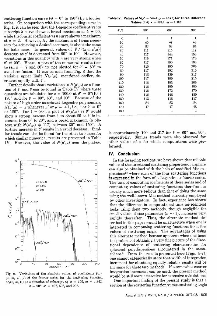
scattering function curve ( = 0 to 1800) by a fourierseries. On comparison with the corresponding curve inFig. 1, it can be seen that the Legendre coefficient vs itssubscript k curve shows a broad maximum at k* 90,while the fourier coefficient vs n curve shows a maximumat n = 2. However, N, the maximum of terms neces-sary for achieving a desired accuracy, is about the samefor both cases. In general, values of Fn(i)(xmu',y)decrease as ' is decreased from 900 to 100. However,variations in this quantity with n are very strong when0' 900. Hence, a part of the numerical results (be-tween n = 7 and 50) are not plotted for 0' = 50 toavoid confusion. It can be seen from Fig. 8 that thevariable upper limit N(M',,), mentioned earlier, de-creases rapidly with 0'.

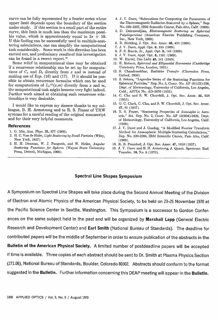
Further details about variations in N(A',A) as a func-tion of 0' and 0 can be found in Table IV where thesequantities are tabulated for x = 100.0 at 0' = 00(100)1800 and for 0 = 300, 600, and 900. Because of thenature of high order associated Legendre polynomials,

= 1 whenever A' or A = 1, i.e., 0 or ' = 0°or 1800. For 0 = 300, a plot of N(,u',,u) vs 0' wouldshow a strong increase from 1 to about 80 as 0' is in-creased from 00 to 200, and a broad maximum (a pla-teau with N,',i) *. 117) between 300 and 1500. Afurther increase in 0' results in a rapid decrease. Simi-lar trends can also be found for the other two cases forwhich similar numerical results are presented in TableIV. However, the value of N(L',M) near the plateau

Table IV. Values of N(,u' = cos 0', ,u = cos 0) for Three DifferentValues of 0; x = 100.0, m = 1.342

0,/0 300 600 90°

0 1 1 110 45 47 4820 83 82 8430 111 115 11740 117 144 15050 116 171 17060 117 190 19070 115 190 20680 117 192 21590 118 189 217

100 117 190 215110 118 193 206120 118 190 190130 118 173 170140 118 148 150150 113 118 117160 84 83 84170 47 47 48180 1 1 1

is approximately 190 and 217 for 0 = 600 and 900,respectively. Similar trends were also observed forother values of x for which computations were per-formed.

IV. Conclusion

10 2

10°

10

-2

10

ICT4

105

-610

0 40 80 120SUBSCRIPT (n)

Fig. 8. Variations of the absolute valuE(x, m, A1', 1u) of the fourier series for thM 2 (x, m, 6) as a function of subscript n;

0 = 900, 0' = 10°, 500, an

In the foregoing sections, we have shown that reliablevalues of the directional scattering properties of a spherecan also be obtained with the help of modified Mie ex-pressions'3 where each of the four scattering functionsis expressed in the form of a Legendre or fourier series.The task of computing coefficients of these series and ofcomputing values of scattering functions therefrom isusually much more tedious than that of doing the sameusing the well-known Mie method currently employedby other investigators. In fact, experience has shownthat the difference in computational time for identicaltasks using these two methods, though negligible for

,=500 small values of size parameter (x - 1), increases veryrapidly thereafter. Thus, the alternate method de-scribed in this paper would be unattractive when one isinterested in computing scattering functions for a fewvalues of scattering angle. The advantages of usingthis alternate method become apparent when one facesthe problem of obtaining a very fine picture of the direc-tional dependence of scattering characteristics forspherical polydispersions encountered in the atmo-sphere.9 From the results presented here (Figs. 4-7),one cannot categorically state that width of integration

200 240 increment for obtaining equally reliable results will bethe same for these two methods. If a somewhat coarser

of coefficients F(l) integration increment can be used, the present methodLe scattering function would be still more attractive for extensive calculations.d = 100, m = 1.342, One important finding of the present study is that aAd 90°. section of the scattering function versus scattering angle

August 1970 / Vol. 9, No. 8 / APPLIED OPTICS 1895

-

curve can be fully represented by a fourier series whoseupper limit depends upon the boundary of the sectionunder study. If this section is a small part of the entirecurve, this limit is much less than the maximum possi-ble value, which is approximately equal to 2x + 10.If this finding can be successfully used in multiple-scat-tering calculations, one can simplify the computationaltask considerably. Some work in this direction has beencarried out, and preliminary results of this investigationcan be found in a recent report.' 7

Some relief in computational time may be obtainedif a recurrence relationship can be set up for computa-tions of C and Dk directly from x and m instead ofmaking use of Eqs. (16) and (17). If it should be pos-sible to obtain recurrence formulas which can be usedfor computations of LU)(x,m) directly from x and m,the computational task might become very light indeed.Further work aimed at obtaining such recurrence rela-tionships is very desirable.

I would like to express my sincere thanks to my col-league, B. H. Armstrong and to R. S. Fraser of TRWsystems for a careful reading of the original manuscriptand for their very helpful comments.

References1. G. Mie, Ann. Phys. 25, 377 (1908).2. H. C. Van de Hulst, Light Scattering by Small Particles (Wiley,

New York, 1957).3. H. H. Denman, W. J. Pangonis, and W. Heller, Angular

Scattering Functions for Spheres (Wayne State UniversityPress, Detroit, Michigan, 1966).

4. J. V. Dave, "Subroutines for Computing the Parameters ofthe Electromagnetic Radiation Scattered by a Sphere," Rep.No. 320-3237, IBM Scientific Center, Palo Alto, Calif. (1968).

5. D. Deirmendjian, Electromagnetic Scattering on SphericalPolydispersions (American Elsevier Publishing Company,Inc., New York, 1969).

6. R. Hickling, J. Opt. Soc. Amer. 58, 455 (1968).7. J. V. Dave, Appl. Opt. 8, 155 (1969).8. F. S. Harris, Jr., Appl. Opt. 8, 143 (1969).9. J. V. Dave, Appl. Opt. 8, 1161 (1969).

10. W. Hartel, Das Licht 40, 141 (1940).11. E. Hobson, Spherical and Ellipsoidal Harmonics (Cambridge

University Press, London, 1931).12. S. Chandrasekhar, Radiative Transfer (Clarendon Press,

Oxford, 1950).13. Z. Sekera, "Legendre Series of the Scattering Functions for

Spherical Particles," Rep. No. 5, Contr. No. AF 19(122)-239,Dept. of Meteorology, University of California, Los Angeles,Calif., ASTIA No. AD-3870 (1952).

14. C. Chu and S. W. Churchill, J. Opt. Soc. Amer. 45, 958(1955).

15. G. C. Clark, C. Chu, and S. W. Churchill, J. Opt. Soc. Amer.47, 81 (1957).

16. R. S. Fraser, "Scattering Properties of Atmosphe ic Aero-sols," Sci. Rep. No. 2, Contr. No. AF 19(604)-2429, Dept.of Meteorology, University of California, Los Angeles, Calif.(1959).

17. J. V. Dave and J. Gazdag, "A Modified Fourier TransformMethod for Atmospheric Multiple Scattering Calculations,"Rep. No. 320-3266, IBM Scientific Center, Palo Alto, Calif.(1969).

18. R. B. Penndorf, J. Opt. Soc. Amer. 47, 1010 (1957).19. J. V. Dave and B. H. Armstrong, J. Quant. Spectrosc. Rad.

Transfer. 10, No. 6 (1970).

Spectral Line Shapes Symposium

A Symposium on Spectral Line Shapes will take place during the Second Annual Meeting of the Division

of Electron and Atomic Physics of the American Physical Society, to be held on 23-25 November 1970 at

the Pacific Science Center in Seattle, Washington. This Symposium is a successor to Gordon Confer-

ences on the same subject held in the past and will be organized by Marshall Lapp (General Electric

Research and Development Center) and Earl Smith (National Bureau of Standards). The deadline for

contributed papers will be the middle of September in order to ensure publication of the abstracts in the

Bulletin of the American Physical Society. A limited number of postdeadline papers will be accepted

if time is available. Three copies of each abstract should be sent to Dr. Smith at Plasma Physics Section

(271.06), National Bureau of Standards, Boulder, Colorado 80302. Abstracts should conform to the format

suggested in the Bulletin. Further information concerning this DEAP meeting will appear in the Bulletin.

1896 APPLIED OPTICS / Vol. 9, No. 8 / August 1970