collider constraints applied to simplified models of dark
TRANSCRIPT
Collider Constraints applied toSimplified Models of Dark Matter fitted
to the Fermi-LAT gamma ray excessusing Bayesian Techniques
Guy Pitman
Department of Physics
University of Adelaide
This dissertation is submitted for the degree of
MPhil
October 2016
I would like to dedicate this thesis to my wife Julia who has enabled this undertaking by herpatience love and support
Declaration
I hereby declare that except where specific reference is made to the work of others thecontents of this dissertation are original and have not been submitted in whole or in partfor consideration for any other degree or qualification in this or any other university Thisdissertation is my own work and contains nothing which is the outcome of work done incollaboration with others except as specified in the text and Acknowledgements Thisdissertation contains fewer than 65000 words including appendices bibliography footnotestables and equations and has fewer than 150 figures
I certify that this work contains no material which has been accepted for the award of anyother degree or diploma in my name in any university or other tertiary institution and to thebest of my knowledge and belief contains no material previously published or written byanother person except where due reference has been made in the text In addition I certifythat no part of this work will in the future be used in a submission in my name for any otherdegree or diploma in any university or other tertiary institution without the prior approval ofthe University of Adelaide and where applicable any partner institution responsible for thejoint-award of this degree I give consent to this copy of my thesis when deposited in theUniversity Library being made available for loan and photocopying subject to the provisionsof the Copyright Act 1968
I acknowledge that copyright of published works contained within this thesis resides withthe copyright holder(s) of those works I also give permission for the digital version of mythesis to be made available on the web via the Universityrsquos digital research repository theLibrary Search and also through web search engines unless permission has been granted bythe University to restrict access for a period of time
Guy PitmanOctober 2016
Acknowledgements
And I would like to acknowledge the help and support of my supervisors Professor TonyWilliams and Dr Martin White as well as Assoc Professor Csaba Balasz who has assisted withinformation about a previous study Ankit Beniwal and Jinmian Li who assisted with runningMicrOmegas and LUXCalc I adapted the collider cuts programs originally developed bySky French and Martin White for my study
Contents
List of Figures xiii
List of Tables xv
1 Introduction 111 Motivation 312 Literature review 4
121 Simplified Models 4122 Collider Constraints 7
2 Review of Physics 921 Standard Model 9
211 Introduction 9212 Quantum Mechanics 9213 Field Theory 10214 Spin and Statistics 10215 Feynman Diagrams 11216 Gauge Symmetries and Quantum Electrodynamics (QED) 12217 The Standard Electroweak Model 13218 Higgs Mechanism 17219 Quantum Chromodynamics 222110 Full SM Lagrangian 23
22 Dark Matter 25221 Evidence for the existence of dark matter 25222 Searches for dark matter 30223 Possible signals of dark matter 30224 Gamma Ray Excess at the Centre of the Galaxy [65] 30
Contents vi
23 Background on ATLAS and CMS Experiments at the Large Hadron collider(LHC) 31231 ATLAS Experiment 32232 CMS Experiment 33
3 Fitting Models to the Observables 3531 Simplified Models Considered 3532 Observables 36
321 Dark Matter Abundance 36322 Gamma Rays from the Galactic Center 36323 Direct Detection - LUX 37
33 Calculations 39331 Mediator Decay 39332 Collider Cuts Analyses 42333 Description of Collider Cuts Analyses 43
4 Calculation Tools 5541 Summary 5542 FeynRules 5643 LUXCalc 5644 Multinest 5745 Madgraph 5846 Collider Cuts C++ Code 59
5 Majorana Model Results 6151 Bayesian Scans 6152 Best fit Gamma Ray Spectrum for the Majorana Fermion DM model 6453 Collider Constraints 67
531 Mediator Decay 67532 Collider Cuts Analyses 69
6 Real Scalar Model Results 7361 Bayesian Scans 7362 Best fit Gamma Ray Spectrum for the Real Scalar DM model 7663 Collider Constraints 77
631 Mediator Decay 77632 Collider Cuts Analyses 78
Contents vii
7 Real Vector Dark Matter Results 8171 Bayesian Scans 8172 Best fit Gamma Ray Spectrum for the Real Vector DM model 8473 Collider Constraints 84
731 Mediator Decay 84732 Collider Cuts Analyses 86
8 Conclusion 89
Bibliography 91
Appendix A Validation of Calculation Tools 97
Appendix B Branching ratio calculations for narrow width approximation 105B1 Code obtained from decayspy in Madgraph 105
List of Figures
21 Feynman Diagram of electron interacting with a muon 1122 Weak Interaction Vertices [48] 1523 Higgs Potential [49] 1824 Standard Model Particles and Forces [50] 2425 Bullet Cluster [52] 2526 Galaxy Rotation Curves [54] 2627 WMAP Cosmic Microwave Background Fluctuations [58] 2928 Dark Matter Interactions [60] 2929 Gamma Ray Excess from the Milky Way Center [75] 31210 ATLAS Experiment 31211 CMS Experiment 34
31 Main Feyman diagrams leading to the cross section for scalar decaying to apair of τ leptons 40
32 WidthmS vs mS 4033 WidthmS vs λb 4134 WidthmS vs λτ 4135 Main Feyman diagrams leading to the cross section for scalar decaying to a
pair of b quarks in the presence of at least one b quark 42
41 Calculation Tools 55
51 Majorana Dark Matter - Posterior probability by individual constraint and alltogether 62
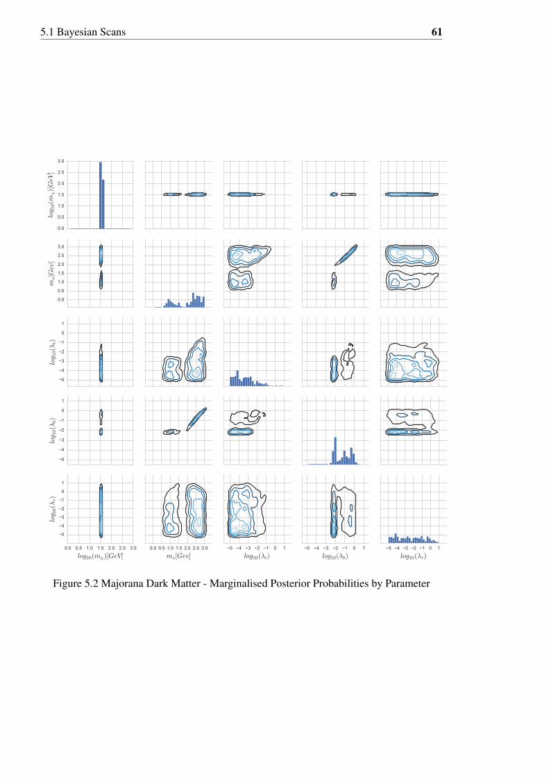
52 Majorana Dark Matter - Marginalised Posterior Probabilities by Parameter 6353 Gamma Ray Spectrum 6454 Plots of log likelihoods by individual and combined constraints Masses in
GeV 6655 σ lowastBr(σ rarr ττ) versus Mass of Scalar 67
List of Figures ix
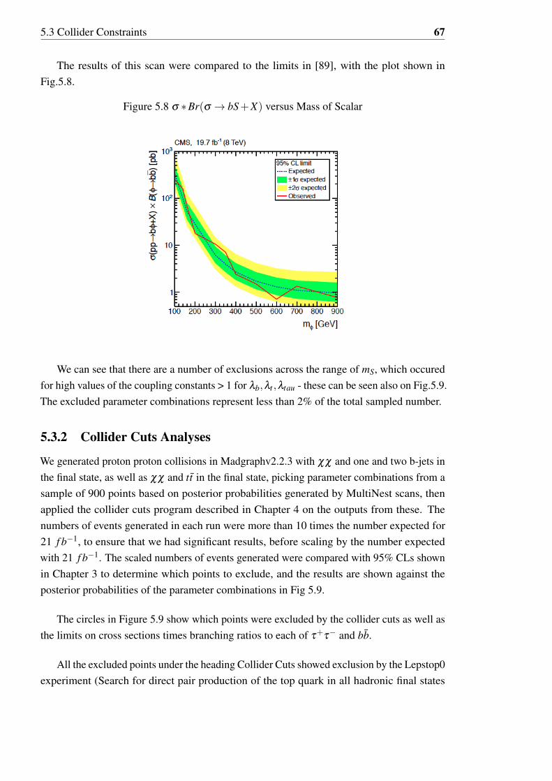
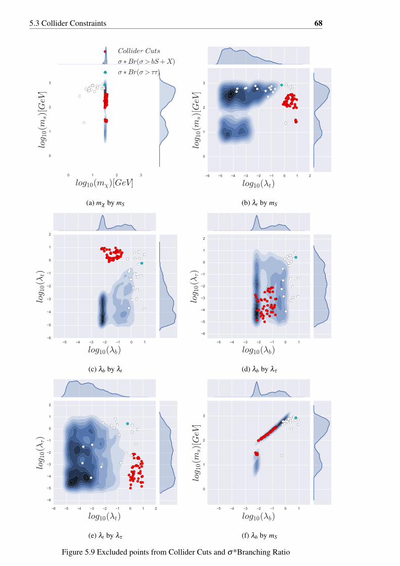
56 σ lowastBr(σ rarr τ+τminus) versus Mass of Scalar 6857 σ lowastBr(σ where rarr bS+X) versus Mass of Scalar 6858 σ lowastBr(σ rarr bS+X) versus Mass of Scalar 6959 Excluded points from Collider Cuts and σBranching Ratio 70
61 Real Scalar Dark Matter - By Individual Constraint and All Together 7462 Real Scalar Matter - Marginalised Posterior Probabilities by Parameter 7563 Gamma Ray Spectrum 7664 σ lowastBr(σ rarr ττ) versus Mass of Scalar 7765 σ lowastBr(σ rarr bS+X) versus Mass of Scalar 7866 Excluded points from Collider Cuts and σBranching Ratio 80
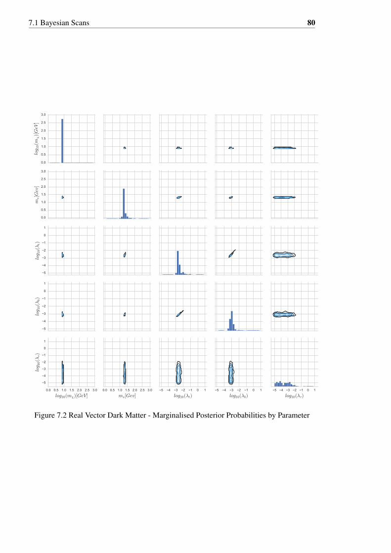
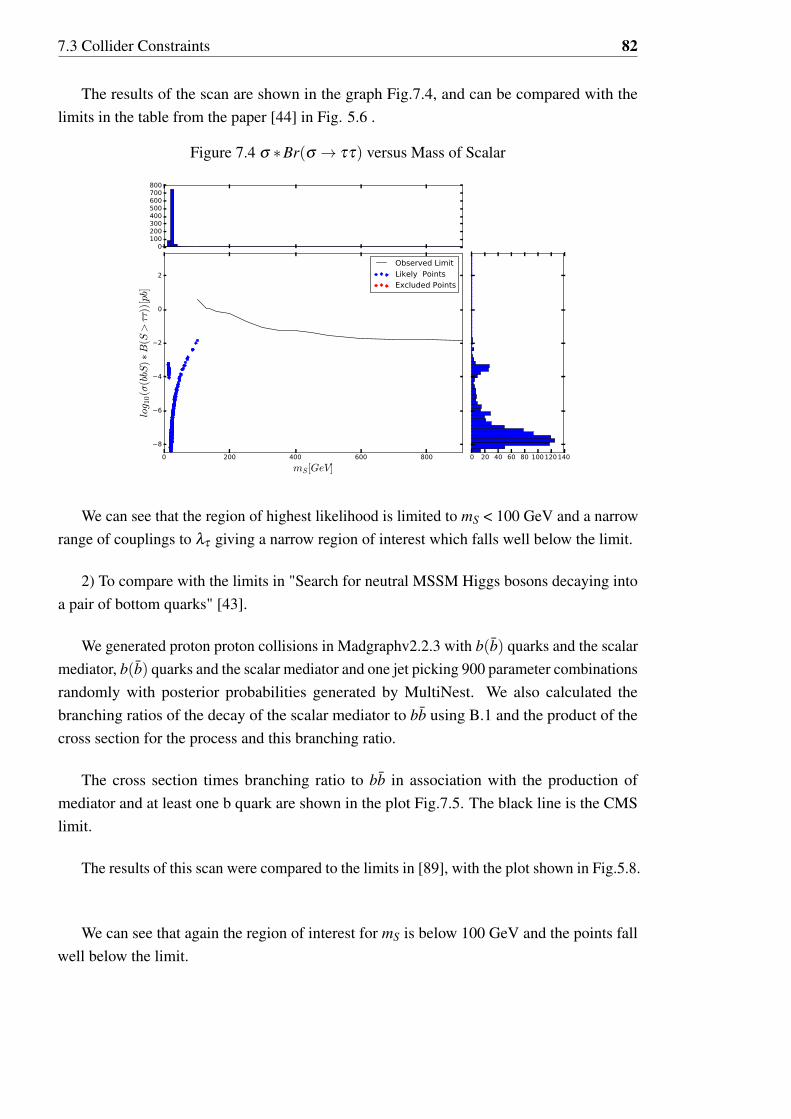
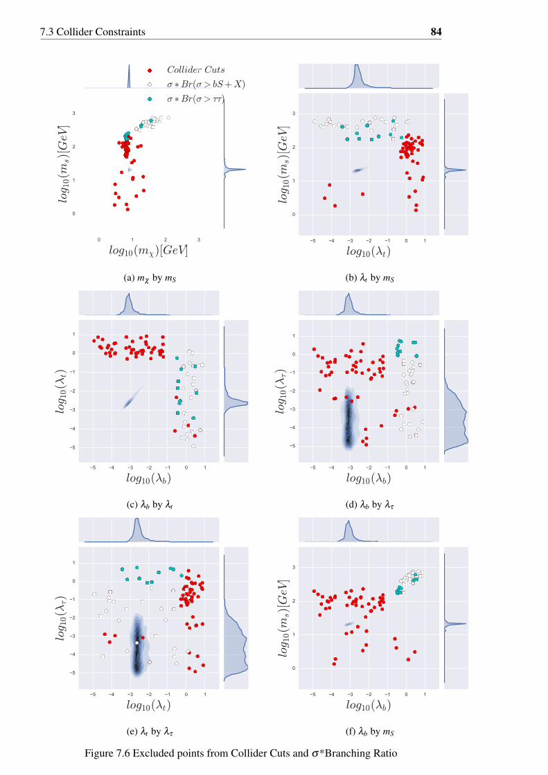
71 Real Vector Dark Matter - By Individual Constraint and All Together 8272 Real Vector Dark Matter - Marginalised Posterior Probabilities by Parameter 8373 Gamma Ray Spectrum 8474 σ lowastBr(σ rarr ττ) versus Mass of Scalar 8575 σ lowastBr(σ rarr bS+X) versus Mass of Scalar 8676 Excluded points from Collider Cuts and σBranching Ratio 87
List of Tables
21 Quantum numbers of the Higgs field 1922 Weak Quantum numbers of Lepton and Quarks 21
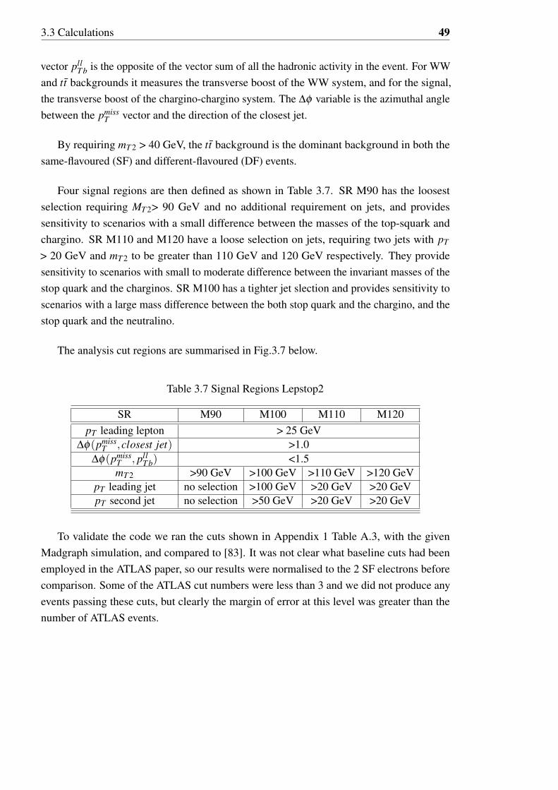
31 Simplified Models 3532 95 CL by Signal Region 4433 Selection criteria common to all signal regions 4534 Selection criteria for signal regions A 4535 Selection criteria for signal regions C 4536 Signal Regions - Lepstop1 4837 Signal Regions Lepstop2 4938 Signal Regions 2bstop 5139 Signal Region ATLASmonobjet 52
51 Scanned Ranges 6152 Best Fit Parameters 64
61 Best Fit Parameters 76
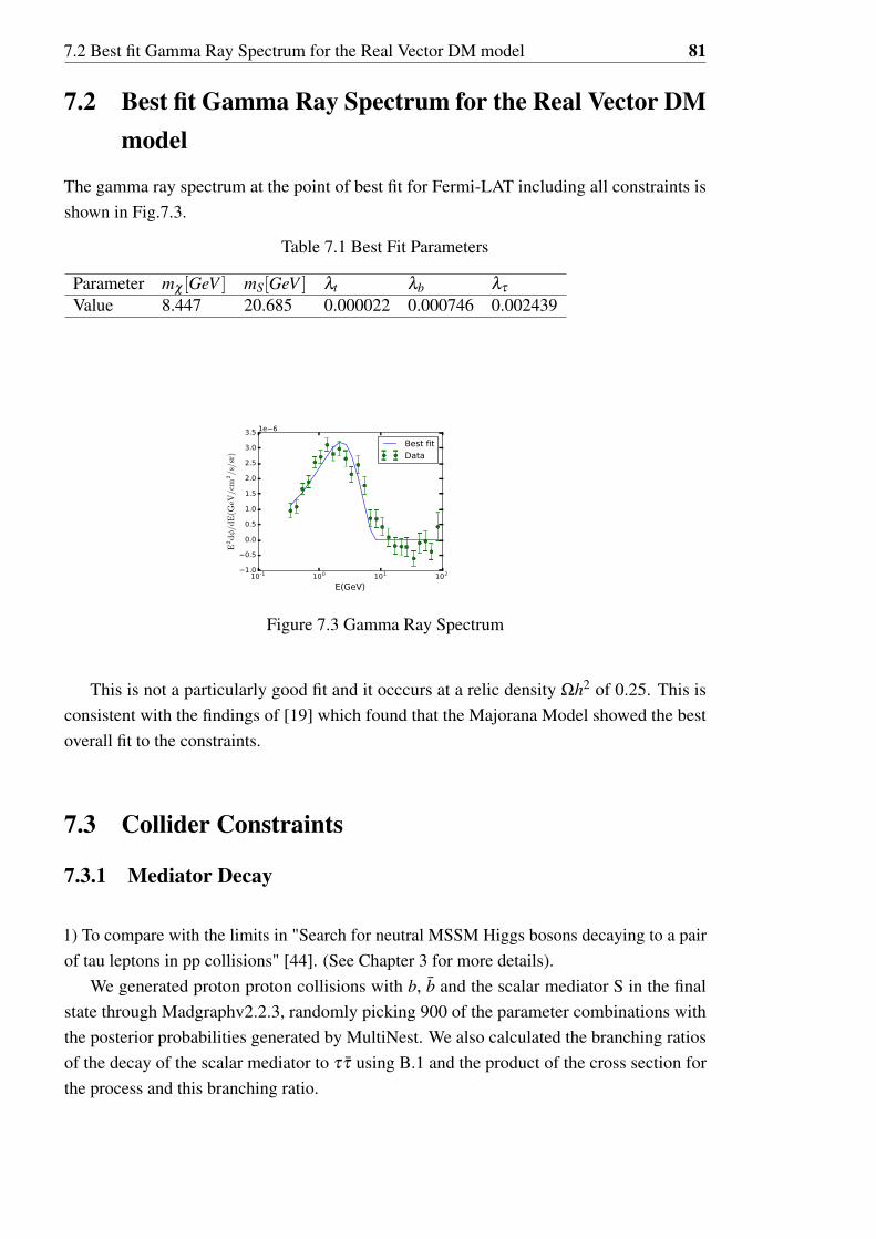
71 Best Fit Parameters 84
A1 0 Leptons in the final state 98A2 1 Lepton in the Final state 100A3 2 Leptons in the final state 101A4 2b jets in the final state 102A5 Signal Efficiencies 90 CL on σ lim
exp[ f b] on pp gt tt +χχ 103
Chapter 1
Introduction
Dark matter (DM) was first postulated over 80 years ago when Swiss astronomer FritzZwicky observed a discrepancy between the amount of light emitted by a cluster of galaxiesand the total mass contained within the cluster inferred from the relative motion of thosegalaxies by a simple application of the theory of Newtonian gravitation The surprising resultof this observation was that the vast majority of the mass in the cluster did not emit lightwhich was contrary to the expectation that most of the mass would be carried by the starsSince that time further observations over a wide range of scales and experimental techniqueshave continued to point to the same result and refine it Some of these observations and otherevidence are discussed in section 22 We now know with certainty that in the entire Universeall of the matter we know about - stars planets gases and other cosmic objects such as blackholes can only account for less than 5 of the mass that we calculate to be there
A recent phenomenon that has received much attention is the significant deviation frombackground expectations of the Fermi Large Area Telescope(Fermi-LAT) gamma ray flux atthe galactic centre [1] A number of astrophysical explanations have been proposed includingmillisecond pulsars of supernova remnants [2] or burst-like continuous events at the galacticcentre but these are unresolved However it has also been noted that the observed Fermi-LATexcess is consistent with the annihilation of dark matter particles which would naturally beconcentrated at the Galactic centre in a manner consistent with the Navarro-Frenk-Whitedistribution of dark matter [3]
There are a number of other purely theoretical (particle physics) reasons to postulatethe existence of weakly interacting matter particles that could supply the missing mass andyet remain unobservable Weakly interacting massive particle (WIMPS) have been a majorfocus of Run I and ongoing Run II searches of the Large Hadron Collider (LHC) In spite
2
of substantial theoretical and experimental effort the microscopic properties of dark matterparticles are still unknown
One of the main problems with extracting these properties is the plethora of competingtheoretical models that provide dark matter candidates Another is the very weak interactionof these particles and the lack of experimental observables allowing one to discriminatebetween the competing models
A particularly fruitful approach is the simplified model approach which makes minimalassumptions about the DM candidates as extensions to the Standard Model interacting weaklywith ordinary matter through a mediator These can be coded as Lagrangian interaction termsusing tools such as FeynRules [4] and Calchep [5] and used to simulate Dark Matter relicdensities indirect detection expectations as well as direct detection expectations throughMicrOmegas [6] This in turn can be run under a Bayesian inference tool (see below)
Using a Bayesian inference tool such as MultiNest [7][8][9] one can scan the parameterspace of a particular model to find regions of highest probability for that model based onobservations of a range of phenomena including direct detection experiments such as ZEPLIN[10] XENON [11] DEAP [12] ARDM [13] DarkSide [14] PandaX [15] and LUX [16]indirect detection - eg Fermi-LAT gamma ray excess [17] Pamela-positron and antiprotonflux [18] and production at colliders MultiNest calculates the evidence value which is theaverage likelihood of the model weighted by prior probability and a posterior distributionwhich is the distribution of the parameter(s) after taking into account the observed databy scanning over a range of parameters based on prior probabilities This can be used tocompare models on a consistent basis The scans also provide information about the best fitparameters for the overall fit as well as for the seperate experimentsobservations
The simplified model approach has been taken in a number of papers to study the Fermi-LAT gamma ray excess (see literature review in section 12) and one in particular comparesthese models using a Bayesian inference tool which found that a Majorana fermion DMcandidate interacting via a scalar mediator with arbitrary couplings to third generationfermions showed the best fit [19] A subsequent paper [20] examined the most likelyparameter combinations that simultaneously fit the Planck relic density Fermi-LAT galacticcentre gamma ray AMS-02 positron flux and Pamela antiproton flux data
There has not as yet been a thorough study of the collider constraints on DM simplifiedmodels that fit the Fermi-LAT galactic centre excess In this thesis we reproduce the
11 Motivation 3
previous results of [20] using similar astrophysical constraints and then implement detailedsimulations of collider constraints on DM and mediator production
In Section 11 we review the motivation for this study and in Section 12 we considerrecent astronomical data which is consistent with the annihilation of DM particles andreview the literature and searches which attempt to explain it with a range of extensions tothe standard model
In Chapter 2 we review the Standard Model of particle physics (SM) the evidence fordark matter and the ATLAS and CMS experiments at the LHC
In Chapter 3 we describe the models considered in this paper the observables used inthe Bayesian scans and the collider experiments which provide limits against which theMagraph simulations of the three models can be compared
In Chapter 4 we review the calculation tools that have been used in this paper
In Chapters 5 6 and 7 we give the results of the Bayesian scans and collider cutsanalyses for each of the models and in Chapter 8 we summarise our conclusions
11 Motivation
The Fermi gamma ray space telescope has over the past few years detected a gamma raysignal from the inner few degrees around the galactic centre corresponding to a regionseveral hundred parsecs in radius The spectrum and angular distribution are compatible withthat from annihilating dark matter particles
A number of papers have recently attempted to explain the Gamma Ray excess in termsof extensions to the Standard Model taking into account constraints from ATLAS and CMScollider experiments direct detection of dark matter colliding off nucleii in well shieldeddetectors (eg LUX) as well as other indirect measurements (astrophysical observations)These papers take the approach of simplified models which describe the contact interactionsof a mediator beween DM and ordinary matter using an effective field theory approach(EFT) Until recently it has been difficult to discriminate between the results of these paperswhich look at different models and produce different statistical results A recent paper[19] Simplified Dark Matter Models Confront the Gamma Ray Excess used a Bayesianinference tool to compare a variety of simplified models using the Bayesian evidence values
12 Literature review 4
calculated for each model to find the most preferred explanation The motivation for thechosen models is discussed in section 121
A subsequent paper [20] Interpreting the Fermi-LAT gamma ray excess in the simplifiedframework studied the most likely model again using Bayesian inference to find the mostlikely parameters for the (most likely) model The data inputs (observables) to the scanwere the Planck measurement of the dark matter relic density [21] Fermi-LAT gamma rayflux data from the galactic center [17] cosmic positron flux data [22] cosmic anti-protonflux data [18] cosmic microwave background data and direct detection data from the LUXexperiment [16] The result of the scan was a posterior probability density function in theparameter space of the model
This paper extends the findings in [19] by adding collider constraints to the likelihoodestimations for the three models It is not a simple matter to add collider constraints becauseeach point in parameter space demands a significant amount of computing to calculate theexpected excess amount of observable particles corresponding to the particular experimentgiven the proposed simplified model A sampling method has been employed to calculatethe collider constraints using the probability of the parameters based on the astrophysicalobservables
12 Literature review
121 Simplified Models
A recent paper [23] summarised the requirements and properties that simplified models forLHC dark matter searches should have
The general principles are
bull Besides the Standard Model (SM) the Lagrangian should contain a DM candidate thatis absolutely stable or lives long enough to escape the LHC detector and a mediatorthat couples the two sectors
bull The Lagrangian should contain all terms that are renormalizable consistent withLorentz invariance SM symmetries and DM stability
bull Additional interactions should not violate exact and approximate global symmetries ofthe SM
12 Literature review 5
The examples of models that satisfy these requirements are
1 Scalar (or pseudo-scalar) s-channel mediator coupled to fermionic dark matter (Diracor Majorana)
2 Higgs portal DM where the DM is a scalar singlet or fermion singlet under the gaugesymmetries of the SM coupling to a scalar boson which mixes with the Higgs (Thefermion singlet is a specific realisation of 1 above)
3 DM is a mixture of an electroweak singlet and doublet as in the Minimal Supersym-metric SM (MSSM)
4 Vector (or Axial vector) s-channel mediator obtained by extending the SM gaugesymmetry by a new U(1)rsquo which is spontaneously broken such that the mediatoracquires mass
5 t-channel flavoured mediator (if the DM particle is a fermion χ the mediator can bea coloured scalar or vector particle φ -eg assuming a scalar mediator a couplingof the form φ χq requires either χ or φ to carry a flavor index to be consistent withminimal flavour violation (MFV) which postulates the flavour changing neutral currentstructure in the SM is preserved
Another recent paper [24] summarised the requirements and properties that simplifiedmodels for LHC dark matter searches should have The models studied in this paper arepossible candidates competing with Dirac fermion and complex scalar dark matter andmodels with vector and pseudo-scalar mediators Other models would have an elasticscattering cross section that will remain beyond the reach of direct detection experiments dueto the neutrino floor (the irreducible background produced by neutrino scattering) or arealready close to sensitivity to existing LUX and XENONIT experiments
A recent paper [25] Scalar Simplified Models for Dark Matter looks at Dirac fermiondark matter mediated by either a new scalar or pseudo-scalar to SM fermions This paperplaces bounds on the coupling combination gχgφ (coupling of DM to mediator times couplingof mediator to SM fermions) calculated from direct detection indirect detection and relicdensity by the mass of DM and mass of mediator Bounds are also calculated for colliderconstraints (mono-jet searches heavy-flavour searches and collider bounds on the 125 GeVHiggs are used to place limits on the monojet and heavy flavor channels which can betranslated into limits on the Higgs coupling to dark matter and experimental measurements
12 Literature review 6
of the Higgs width are used to constrain the addition of new channels to Higgs decay) Thepaper models the top loop in a full theory using the Monte Carlo generator MCFM [26]and extends the process to accommodate off-shell mediator production and decay to a darkmatter pair While this paper does not consider the Majorana fermion dark matter model theconstraints on the coupling product may have some relevence to the present study if only asan order of magnitude indicator
Constraining dark sectors with monojets and dijets [27] studies a simplified model withDirac fermion dark matter and an axial-vector mediator They use two classes of constraint-searches for DM production in events with large amounts of missing transverse energy inassociation with SM particles (eg monojet events) and direct constraints on the mediatorfrom monojet searches to show that for example where the choice of couplings of themediator to quarks and DM gA
q =gAχ=1 all mediator masses in the range 130 GeV ltMR lt3
TeV are excluded
The paper Constraining Dark Sectors at Colliders Beyond the Effective Theory Ap-proach [28] considers Higgs portal models with scalar pseudo-scalar vector and axial-vectormediators between the SM and the dark sector The paper takes account of loop processesand gluon fusion as well as quark-mediator interactions using MCFM Apart from mediatortype the models are characterised by free parameters of mediator width and mass darkmatter mass and the effective coupling combination gχgφ (coupling of DM to mediator timescoupling of mediator to SM fermions) The conclusion is that LHC searches can proberegions of the parameter space that are not able to be explored in direct detection experiments(since the latter measurements suffer from a velocity suppression of the WIMP-nucleoncross-section)
The paper Constraining the Fermi-LAT excess with multi-jet plus EmissT collider searches
[29] shows that models with a pseudo-scalar or scalar mediator are best constrained by multi-jet final states with Emiss
T The analysis was done using POWHEG-BOX-V2 at LO and usesM2
T variables together with multi-jet binning to exploit differences in signal and backgroundin the different regions of phase space to obtain a more stringent set of constraints on DMproduction This paper largely motivated the current work in that it showed that collidersearches that were not traditionally thought of as dark matter searches were neverthelessoften sensitive to dark matter produced in association with heavy quarks The combinationof searches used in this paper reflects this fact
12 Literature review 7
122 Collider Constraints
In order to constrain this model with collider constraints (direct detection limits) we considerthe following papers by the CMS and ATLAS collaborations which describe searches at theLHC
ATLAS Experiments
bull Search for dark matter in events with heavy quarks and missing transverse momentumin p p collisions with the ATLAS detector [30]
bull Search for direct third-generation squark pair production in final states with missingtransverse momentum and two b-jets in
radics= 8 TeV pp collisions with the ATLAS
detector[31]
bull Search for direct pair production of the top squark in all-hadronic final states inprotonndashproton collisions at
radics=8 TeV with the ATLAS detector [32]
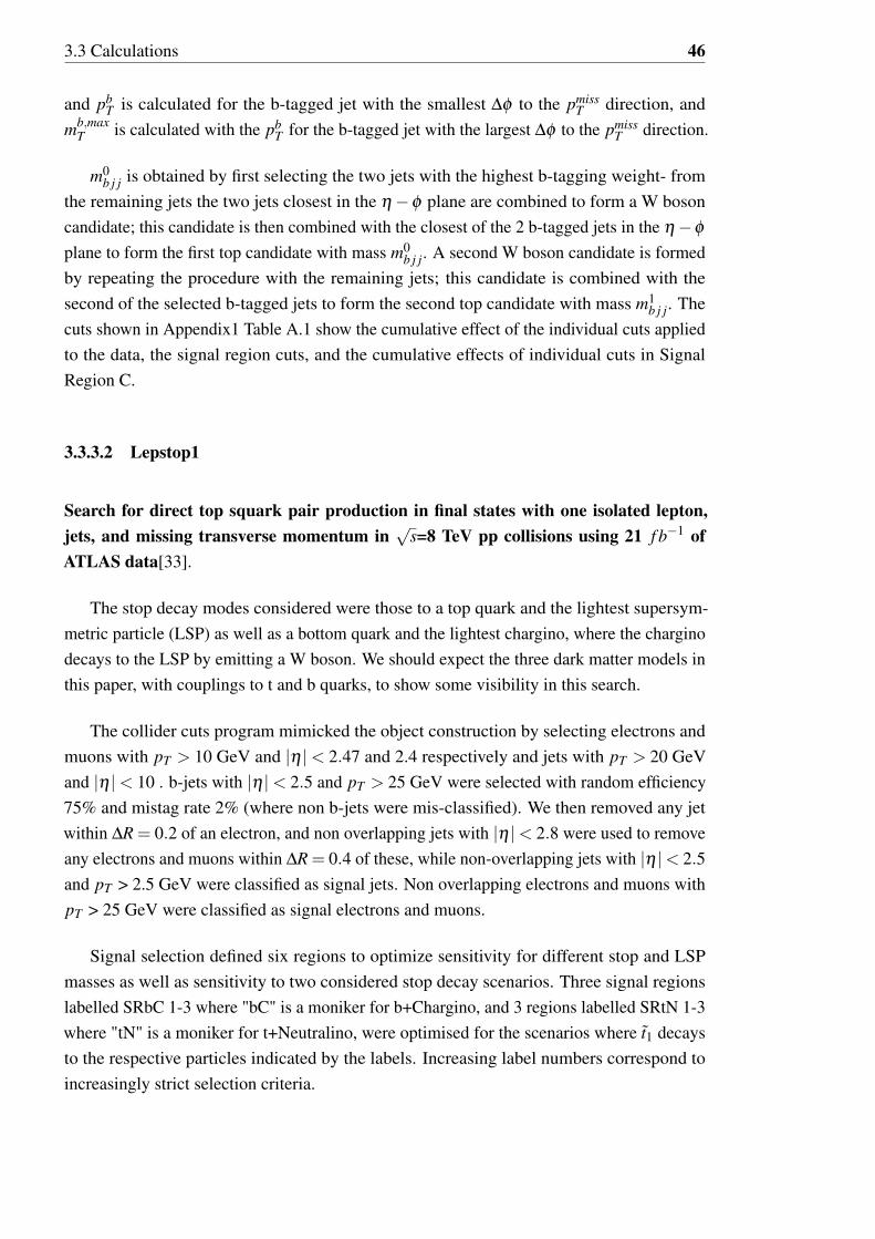
bull Search for direct top squark pair production in final states with one isolated leptonjets and missing transverse momentum in
radic(s)=8TeV pp collisions using 21 f bminus1 of
ATLAS data [33]
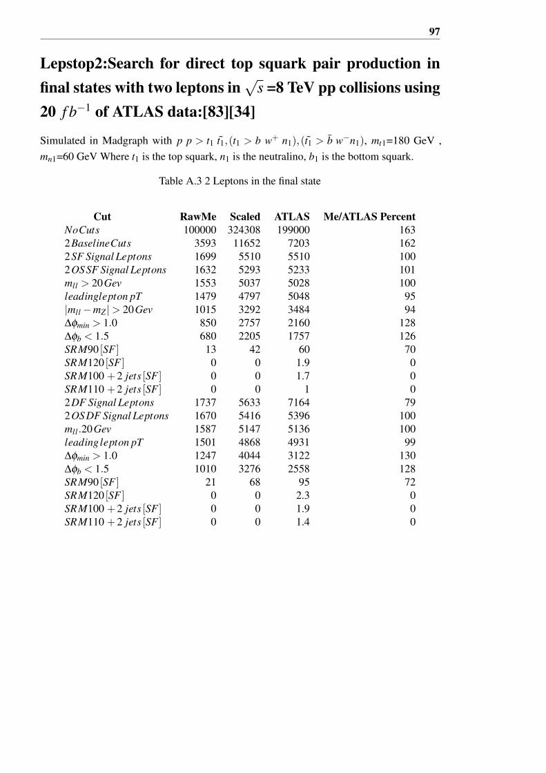
bull Search for direct top squark pair production in final states with two leptons inradic
s = 8TeV pp collisions using 20 f bminus1 of ATLAS data [34]
bull Search for the Production of Dark Matter in Association with Top Quark Pairs in theDi-lepton Final State in pp collisions at
radics=8 TeV [35]
CMS Experiments
bull Searches for anomalous tt production in p p collisions atradic
s=8 TeV [36]
bull Search for the Production of Dark Matter in Association with Top Quark Pairs in theDi-lepton Final State in pp collisions at
radics=8 TeV [37]
bull Search for the production of dark matter in association with top-quark pairs in thesingle-lepton final state in proton-proton collisions at
radics = 8 TeV [38]
bull Search for new physics in monojet events in p p collisions atradic
s = 8 TeV(CMS) [39]
bull Search for new phenomena in monophoton final states in proton-proton collisions atradic
s = 8 TeV [40]
12 Literature review 8
bull Search for the Production of Dark Matter in Association with Top Quark Pairs in theSingle-lepton Final State in pp collisions at
radics=8 TeV [41]
bull Search for new phenomena in monophoton final states in proton-proton collisions atradic
s=8 TeV [42]
bull Search for neutral MSSM Higgs bosons decaying into a pair of bottom quarks [43]
bull Search for neutral MSSM Higgs bosons decaying into a pair of τ leptons in p p collision[44]
bull Search for dark matter extra dimensions and unparticles in monojet events in proton-proton collisions at
radics=8 TeV [45]
In particular we have implemented Madgraph simulations of certain data analysesapplying to collider experiments described in papers [32][33][34][31][30][41] Theremaining models were not implemented in Madgraph because of inability to validate themodels against published results in the time available We developed C++ analysis code toimplement the collider cuts after showering with Pythia and basic analysis with Delpheswith output to root files The C++ code allowed multiple experimental cuts to be applied tothe same simulation output The C++ code was first checked against the results of the variousexperiments above and then the simulations were rerun using the three modelsrsquo Lagrangians(implemented in FeynRules) described in this paper
Chapter 2
Review of Physics
21 Standard Model
211 Introduction
The Standard Model of particle physics (SM) has sometimes been described as the theoryof Almost Everything The SM is a field theory which emerged in the second half of thetwentieth century from quantum mechanics and special relativity which themselves wereonly conceived after 1905 by Einsten Pauli Bohr Dirac and others In the first decades ofthe twenty first century the discovery of the Higgs boson [46][47] completed the pictureand confirmed the last previously unverified part of the SM The SM is a self consistenttheory that describes and classifies all known particles and their interactions (other thangravity) to an astonishing level of accuracy and detail However the theory is incomplete-it does not describe the complete theory of gravitation or account for DM (see below) ordark energy (the accelerating expansion of the universe) Related to these shortcomings aretheoretical deficiencies such as the asymmetry of matter and anti-matter the fact that the SMis inconsistent with general relativity (to the extent that one or both theories break down atspacetime singularities like the Big Bang and black hole event horizons)
212 Quantum Mechanics
Quantum Mechanics (QM) describes particles as probability waves which can be thoughtof as packets of energy which can be localised or spread through all space depending on how
21 Standard Model 10
accurately one measures the particlersquos momentum However QM is not itself consistent withspecial relativity It was realised too that because of relativity particles could be created anddestroyed and because of the uncertainty principle the theory should describe the probabilityof particles being created and destroyed on arbitrarily short timescales A quantum fieldtheory (QFT) is a way to describe this probability at every point of space and time
213 Field Theory
A field theory is described by a mathematical function of space and time called a LagrangianAs in classical mechanics where Lagrangians were introduced by Louis Lagrange at thebeginning of the nineteenth century to summarise dynamical systems the Lagrangian sum-marises the dynamics of space which is permeated by force fields The equations of motionarising from a Lagrangian are determined by finding the contours of the Lagrangian describedby stationary points (ie where the infinitesimal change in the Lagrangian is zero for a smallchange in field) Particles are generally described by singularities in the Lagrangian (wherethe values tend to infinity also called resonances)
214 Spin and Statistics
It was also realised that different types of particle needed to be represented by different fieldsin the Lagrangian Diracrsquos discovery that particles with spin 12 quantum numbers couldbe represented by a field obtained by effectively taking the square root of the relativisticequation (Klein Gordon equation) was probably the most significant advance in quantumfield theory It required the introduction of a matrix operators called the gamma matricesor Dirac matrices which helped explain the already known fact that spin half particles orfermions obey Fermi-Dirac statistics ie when two spin half particles are exchanged thesign of the wavefunction must change and hence they cannot occupy the same quantum stateunlike bosons with integer spin that can occupy the same quantum state
Other particles need to be represented by fields called vector pseudo-vector scalar (as inthe Klein Gordon equation) pseudo-scalar and complex fields A vector field is really fourfields one for each dimension of space plus time and is parameterised by the four gammamatrices γmicro which transform among themselves in a relativistically invariant way (Lorentzinvariance) A pseudo-vector field is a vector field which transforms in the same way but
21 Standard Model 11
with additional sign change under parity transformations (a simultaneous reversal of the threespatial directions) and is represented by γmicroγ5 A pseudo-scalar is a scalar which changes signunder parity transformations and a complex scalar field is represented by complex numbers
215 Feynman Diagrams
QFT took another giant leap forward when Richard Feynman realised that the propagationof particles described by the field could be described by expanding the so called S-matrixor scattering matrix derived from calculating the probability of initial states transitioning tofinal states The expansion is similar to a Taylor expansion in mathematics allowing for thespecial commuting properties of elements of the field The Feynman diagrams representingindividual terms in the expansion can be interpreted as interactions between the particlecomponents The S-Matrix (or more correctly the non trivial part called the T-Matrix) isderived using the interaction Hamiltonian of the field The Hamiltonian is an operator whoseeigenvalues or characteristic values give the energy quanta of the field The T-matrix canalso be described by a path integral which is an integral over all of quantum space weightedby the exponential of the Lagrangian This is completely equivalent to the Hamiltonianformulation and shows how the Lagrangian arises naturally out of the Hamiltonian (in factthe Lagrangian is the Legendre transformation of the Hamiltonian)
Figure 21 Feynman Diagram of electron interacting with a muon
γ
eminus
e+
micro+
microminus
The diagram Fig21 is a tree diagram (diagrams with closed loops indicate self in-teractions and are higher order terms in the expansion) and shows an electron (eminus) and ananti-muon (micro+) interacting by exchanging a photon
21 Standard Model 12
216 Gauge Symmetries and Quantum Electrodynamics (QED)
The Dirac equation with its gamma matrices ushered in the use of group theory to describethe transformation of fields (because the multiplication table of the gamma matrices isclosed and described by group theory) It also ushered in the idea of symmetries within theLagrangian- for example consider a Lagrangian
ψ(ipart minusm)ψ (21)
The Lagrangian is invariant under a global U(1) transformation which acts on the fieldsand hence the derivatives as follows
ψ rarr eiqαψ ψ rarr ψeminusiqα partmicroψ rarr eiqα
partmicroψ (22)
where qα is a global phase and α is a continuous parameter
A symmetry leads by Noetherrsquos theorem to a conserved current jmicro = qψγmicroψ and is thebasis of charge conservation since partmicro jmicro = 0 and q =
intd3x j0(x)
By promoting this transformation to a local one (ie α rarr α(x) where x = xmicro are thespace time co-ordinates) the transformations become
ψ rarr eiqα(x)ψ ψ rarr ψeminusiqα(x)partmicroψ rarr eiqα(x)(partmicroψ + iq(partmicroα(x))ψ) (23)
The derivative transformation introduces an extra term which would spoil the gaugeinvariance This can be solved by introducing a new field the photon field Amicro(x) whichinteracts with the fermion field ψ and transforms under a U(1) transformation
Amicro rarr Amicro minuspartmicroα(x) (24)
If we replace normal derivatives partmicro with covariant derivatives Dmicro = (partmicro + iqAmicro(x)) in theLagrangian then the extra term is cancelled and we can now see that the covariant derivativetransforms like ψ - under a local U(1) transform ie
Dmicro rarr Dmicroψprime = eiqα(x)Dmicroψ (25)
The additional term iqAmicro(x) can be interpreted in a geometric sense as a connectionwhich facilitates the parallel transport of vectors along a curve in a parallel consistent manner
21 Standard Model 13
We must add a gauge-invariant kinetic term to the Lagrangian to describe the dynamicsof the photon field This is given by the electromagnetic field strength tensor
Fmicroν = partmicroAν minuspartνAmicro (26)
The full Quantum Electrodynamics (QED) Lagrangian is then for electrons with mass mand charge -e
LQED = ψ(i Dminusm)ψ minus 14
Fmicroν(X)Fmicroν(x) (27)
This Lagrangian is Lorentz and U(1) guage invariant The interaction term is
Lint =+eψ Aψ = eψγmicro
ψAmicro = jmicro
EMAmicro (28)
where jmicro
EM is the electromagnetic four current
217 The Standard Electroweak Model
The Standard Electroweak (EW) Model was created by Glashow-Weinberg-Salam (also calledthe GWS model) and unifies the electomagnetic and weak interactions of the fundamentalparticles
The idea of gauge symmetry was extended to the idea of a non-abelian gauge symmetry(essentially the operators defining the symmetry do not commute and so are represented bymatrices- in this case the Pauli matrices for the SU(2) group) - the gauge group is the directproduct G = SU(2)
otimesU(1) It was known that weak interactions were mediated by Wplusmn
and Z0 particles where the superscripts are the signs of the electromagnetic charge Thesewere fairly massive but it was also known that through spontaneous symmetry breaking ofa continuous global non-abelian symmetry there would be one massive propagation modefor each spontaneously broken-symmetry generator and massless modes for the unbrokengenerators (the so-called Goldstone bosons)
This required an extra field to represent the gauge bosons called Bmicro (a vector fieldhaving the 4 spacetime degrees of freedom) With this identification the covariant derivativebecomes
Dmicro = partmicro minus igAmicro τ
2minus i
gprime
2Y Bmicro (29)
21 Standard Model 14
Here Y is the so called weak hypercharge of the field Bmicro which is a quantum numberdepending on particle (lepton or quark) g and gprime are two independent parameters in theGWS theory and the expression Amicro τ implies a sum over 3 components Aa
micro a=123 and thePauli matrices τa
This isnrsquot the full story because it had been known since 1956 when Chin Shuing Wuand her collaborators confirmed in an experiment prompted by Lee and Yang that nature isnot ambivalent to so-called parity It had been assumed that the laws of nature would notchange if all spatial coordinates were reversed (a parity transformation) The experimentinvolved the beta decay of cooled 60C atoms (more electrons were emitted in the backwardhemisphere with respect to spin direction of the atoms) This emission involved the weakinteraction and required that the Lagrangian for weak interactions contain terms which aremaximally parity violating- which turn out to be currents of the form
ψ(1minus γ5)γmicro
ψ (210)
The term
12(1minus γ
5) (211)
projects out a left-handed spinor and can be absorbed into the spinor to describe left-handedleptons (and as later discovered quarks) The right handed leptons are blind to the weakinteraction
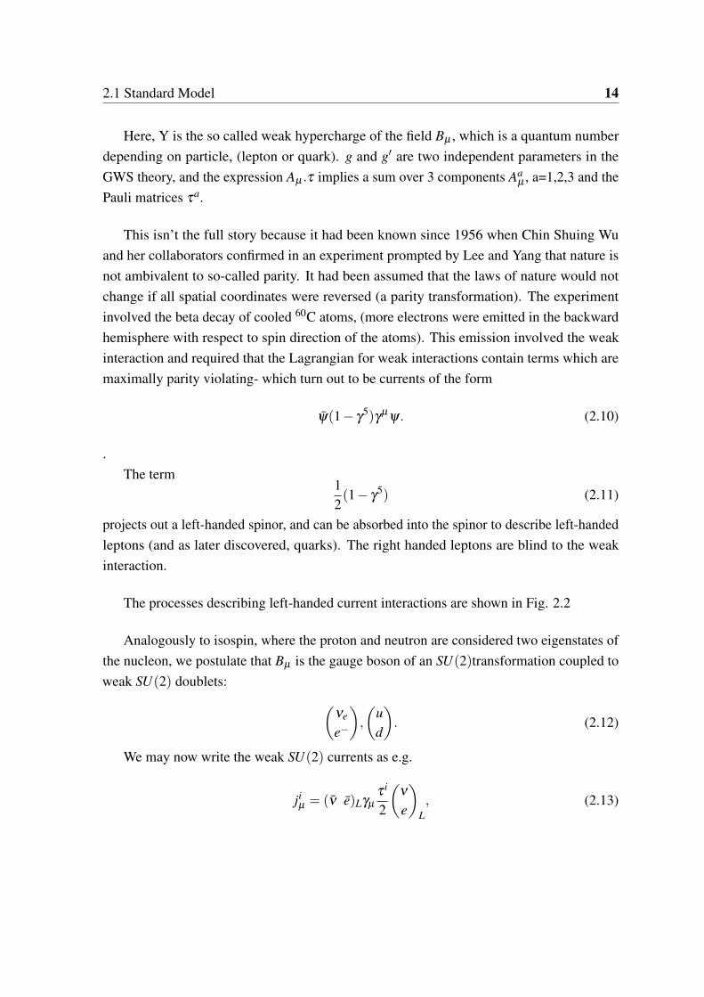
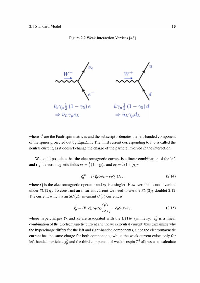
The processes describing left-handed current interactions are shown in Fig 22
Analogously to isospin where the proton and neutron are considered two eigenstates ofthe nucleon we postulate that Bmicro is the gauge boson of an SU(2)transformation coupled toweak SU(2) doublets (
νe
eminus
)
(ud
) (212)
We may now write the weak SU(2) currents as eg
jimicro = (ν e)Lγmicro
τ i
2
(ν
e
)L (213)
21 Standard Model 15
Figure 22 Weak Interaction Vertices [48]
where τ i are the Pauli-spin matrices and the subscript L denotes the left-handed componentof the spinor projected out by Eqn211 The third current corresponding to i=3 is called theneutral current as it doesnrsquot change the charge of the particle involved in the interaction
We could postulate that the electromagnetic current is a linear combination of the leftand right elecromagnetic fields eL = 1
2(1minus γ5)e and eR = 12(1+ γ5)e
jemmicro = eLγmicroQeL + eRγmicroQeR (214)
where Q is the electromagnetic operator and eR is a singlet However this is not invariantunder SU(2)L To construct an invariant current we need to use the SU(2)L doublet 212The current which is an SU(2)L invariant U(1) current is
jYmicro = (ν e)LγmicroYL
(ν
e
)L+ eRγmicroYReR (215)
where hypercharges YL and YR are associated with the U(1)Y symmetry jYmicro is a linearcombination of the electromagnetic current and the weak neutral current thus explaining whythe hypercharge differs for the left and right-handed components since the electromagneticcurrent has the same charge for both components whilst the weak current exists only forleft-handed particles j3
micro and the third component of weak isospin T 3 allows us to calculate
21 Standard Model 16
the relationship Y = 2(QminusT 3) which can be seen by writing jYmicro as a linear combination ofj3micro (the weak neutral current that doesnrsquot change the charge of the particle involved in the
interaction) and jemmicro (using the convention that the jYmicro is multiplied by 1
2 to match the samefactor implicit in j3
micro ) Substituting
τ3 =
(1 00 minus1
)(216)
into equation 213 for i=3 and subtracting equation 215 and equating to 12 times equation
214
we get
eLγmicroQeL + eRγmicroQeR minus (νLγmicro
12
νL minus eLγmicro
12
eL) =12
eRγmicroYReR +12(ν e)LγmicroYL
(ν
e
)L (217)
from which we can read out
YR = 2QYL = 2Q+1 (218)
and T3(eR) = 0 T3(νL) =12 and T3(eL) =
12 The latter three identities are implied by
the fraction 12 inserted into the definition of equation 213
The Lagrangian kinetic terms of the fermions can then be written
L =minus14
FmicroνFmicroν minus 14
GmicroνGmicroν
+ sumgenerations
LL(i D)LL + lR(i D)lR + νR(i D)νR
+ sumgenerations
QL(i D)QL +UR(i D)UR + DR(i D)DR
(219)
LL are the left-handed lepton doublets QL are the left-handed quark doublets lRνR theright handed lepton singlets URDR the right handed quark singlets
The field strength tensors are given by
Fmicroν = partmicroAν minuspartνAmicro minus ig[Amicro Aν ] (220)
21 Standard Model 17
andGmicroν = partmicroBν minuspartνBmicro (221)
Bmicro is an abelian U(1) gauge field while Amicro is non-abelian and Fmicroν contains the com-mutator of the field through the action of the covariant derivative [Dmicro Dν ] This equationcontains no mass terms terms for the field Amicro for good reason- this would violate gaugeinvariance We know that the gauge bosons of the weak force have substantial mass and theway that this problem has been solved is through the Higgs mechanism
218 Higgs Mechanism
To solve the problem of getting gauge invariant mass terms three independent groupspublished papers in 1964 The mechanism was named after Peter Higgs To introduce theconcept consider a complex scalar field φ that permeates all space Consider a potential forthe Higgs field of the form
minusmicro2φ
daggerφ +λ (φ dagger
φ2) (222)
which has the form of a mexican hat Fig 23 This potential is still U(1) gauge invariant andcan be added to our Lagrangian together with kinetic+field strength terms to give
L = (Dmicroφ)dagger(Dmicroφ)minusmicro2φ
daggerφ +λ (φ dagger
φ2)minus 1
4FmicroνFmicroν (223)
It is easily seen that this is invariant to the transformations
Amicro rarr Amicro minuspartmicroη(x) (224)
φ(x)rarr eieη(x)φ(x) (225)
The minimum of this field is not at 0 but in a circular ring around 0 with a vacuum
expectation value(vev)radic
micro2
2λequiv vradic
2
We can parameterise φ as v+h(x)radic2
ei π
Fπ where h and π are referred to as the Higgs Bosonand Goldstone Boson respectively and are real scalar fields with no vevs Fπ is a constant
21 Standard Model 18
Figure 23 Higgs Potential [49]
Substituting this back into the Lagrangian 223 we get
minus14
FmicroνFmicroν minusevAmicropartmicro
π+e2v2
2AmicroAmicro +
12(partmicrohpart
microhminus2micro2h2)+
12
partmicroπpartmicro
π+(hπinteractions)(226)
This Lagrangian now seems to describe a theory with a photon Amicro of mass = ev a Higgsboson h with mass =
radic2micro and a massless Goldstone π
However there is a term mixing Amicro and part microπ in this expression and this shows Amicro and π
are not independent normal coordinates and we can not conclude that the third term is a massterm This π minusAmicro mixing can be removed by making a gauge transformation in equations224 and 225 making
φrarrv+h(x)radic2
ei π
Fπminusieη(x) (227)
and setting πrarr π
Fπminus eη(x) = 0 This choosing of a point on the circle for the vev is called
spontaneous symmetry breaking much like a vertical pencil falling and pointing horizontallyin the plane This choice of gauge is called unitary gauge The Goldstone π will thencompletely disappear from the theory and one says that the Goldstone has been eaten to givethe photon mass
21 Standard Model 19
This can be confirmed by counting degrees of freedom before and after spontaneoussymmetry breaking The original Lagrangian had four degrees of freedom- two from thereal massless vector field Amicro (massless photons have only two independent polarisationstates) and two from the complex scalar field (one each from the h and π fields) The newLagrangian has one degree of freedom from the h field and 3 degrees of freedom from themassive real vector field Amicro and the π field has disappeared
The actual Higgs field is postulated to be a complex scalar doublet with four degrees offreedom
Φ =
(φ+
φ0
)(228)
which transforms under SU(2) in the fundamental representation and also transforms underU(1) hypercharge with quantum numbers
Table 21 Quantum numbers of the Higgs field
T 3 Q Yφ+
12 1 1
φ0 minus12 1 0
We can parameterise the Higgs field in terms of deviations from the vacuum
Φ(x) =(
η1(x)+ iη2(x)v+σ(x)+ iη3(x)
) (229)
It can be shown that the three η fields can be transformed away by working in unitarygauge By analogy with the scalar Higgs field example above the classical action will beminimised for a constant value of the Higgs field Φ = Φ0 for which Φ
dagger0Φ0 = v2 This again
defines a range of minima and we can pick one arbitarily (this is equivalent to applying anSU(2)timesU(1) transform to the Higgs doublet transforming the top component to 0 and thebottom component to Φ0 = v) which corresponds to a vacuum of zero charge density andlt φ0 gt=+v
In this gauge we can write the Higgs doublet as
Φ =
(φ+
φ0
)rarr M
(0
v+ H(x)radic2
) (230)
where H(x) is a real Higgs field v is the vacuum expectation and M is an SU(2)timesU(1)matrix The matrix Mdagger converts the isospinor into a down form (an SU(2) rotation) followedby a U(1) rotation to a real number
21 Standard Model 20
If we consider the Higgs part of the Lagrangian
minus14(Fmicroν)
2 minus 14(Bmicroν)
2 +(DmicroΦ)dagger(DmicroΦ)minusλ (Φdagger
Φminus v2)2 (231)
Substituting from equation 230 into this and noting that
DmicroΦ = partmicroΦminus igW amicro τ
aΦminus 1
2ig
primeBmicroΦ (232)
We can express as
DmicroΦ = (partmicro minus i2
(gA3
micro +gprimeBmicro g(A1micro minusA2
micro)
g(A1micro +A2
micro) minusgA3micro +gprimeBmicro
))Φ equiv (partmicro minus i
2Amicro)Φ (233)
After some calculation the kinetic term is
(DmicroΦ)dagger(DmicroΦ) =12(partH)2 +
14(v+
Hradic2)2[A 2]22 (234)
where the 22 subscript is the index in the matrix
If we defineWplusmn
micro =1radic2(A1
micro∓iA2micro) (235)
then [A 2]22 is given by
[A 2]22 =
(gprimeBmicro +gA3
micro
radic2gW+
microradic2gWminus
micro gprimeBmicro minusgA3micro
) (236)
We can now substitute this expression for [A 2]22 into equation 234 and get
(DmicroΦ)dagger(DmicroΦ) =12(partH)2 +
14(v+
Hradic2)2(2g2Wminus
micro W+micro +(gprimeBmicro minusgA3micro)
2) (237)
This expression contains mass terms for three massive gauge bosons Wplusmn and the combi-nation of vector fields gprimeBmicro minusgA3
micro where note
21 Standard Model 21
Table 22 Weak Quantum numbers of Lepton and Quarks
T 3 Q YνL
12 0 -1
lminusL minus12 -1 -1
νR 0 0 0lminusR 0 -1 -2UL
12
23
13
DL minus12 minus1
313
UR 0 23
43
DR 0 minus13 minus2
3
Wminusmicro = (W+
micro )dagger equivW 1micro minus iW 2
micro (238)
Then the mass terms can be written
12
v2g2|Wmicro |2 +14
v2(gprimeBmicro minusgA3micro)
2 (239)
W+micro and W microminus can be associated with the W boson and its anti-particle and (minusgprimeBmicro +
gA3micro) with the Z Boson (after normalisation by
radicg2 +(gprime
)2) The combination gprimeA3micro +gBmicro
is orthogonal to Z and remains massless This can be associated with the Photon (afternormalisation) These predict mass terms for the W and Z bosons mW = vgradic
2and mZ =
vradic2
radicg2 +(gprime
)2It is again instructive to count the degrees of freedom before and after the Higgs mech-
anism Before we had a complex doublet Φ with four degrees of freedom one masslessB with two degrees of freedom and three massless W a fields each with two each givinga total of twelve degrees of freedom After spontaneous symmetry breaking we have onereal scalar Higgs field with one degree of freedom three massive weak bosons with nineand one massless photon with two again giving twelve degrees of freedom One says thescalar degrees of freedom have been eaten to give the Wplusmn and Z bosons their longitudinalcomponents (ie mass)
Table 22 shows T 3 the weak isospin quantum number (which describes how a particletransforms under SU(2)) Y the weak hypercharge (which describes how the particle trans-
21 Standard Model 22
forms under U(1)) and Q the electric charge of leptons and quarks The former two enterdirectly into the Lagrangian while the latter can be derived as a function of the former two
Strictly speaking the right handed neutrino which has no charge may not exist and is notpart of the standard model although some theories postulate a mass for this (hypothetical)particle
Writing gauge invariant couplings between ELeRφ with the vacuum expectation ofφ = v (Yukawa matrices λ
i ju and λ
i jd respectively for the up and down quarks) we get mass
terms for the quarks (and similarly for the leptons)
Mass terms for quarks minussumi j[(λi jd Qi
Lφd jR)+λ
i ju εab(Qi
L)aφlowastb u j
R +hc]
Mass terms for leptonsminussumi j[(λi jl Li
Lφ l jR)+λ
i jν εab(Li
L)aφlowastb ν
jR +hc]
Here hc is the hermitian conjugate of the first terms L and Q are lepton and quarkdoublets l and ν are the lepton singlet and corresponding neutrino d and u are singlet downand up quarks εab is the Levi-Civita (anti-symmetric) tensor
If we write the quark generations in a basis that diagonalises the Higgs couplings weget a unitary transformations Uu and Ud for the up and down quarks respectively which iscompounded in the boson current (Udagger
u Ud) called the CKM matrix where off-diagonal termsallow mixing between quark generations (this is also called the mass basis as opposed tothe flavour basis) A similar argument can give masses to right handed sterile neutrinos butthese can never be measured However a lepton analogue of the CKM matrix the PNMSmatrix allows left-handed neutrinos to mix between various generations and oscillate betweenflavours as they propagate through space allowing a calculation of mass differences
219 Quantum Chromodynamics
The final plank in SM theory tackling the strong force Quantum Chromodynamics wasproposed by Gell-Mann and Zweig in 1963 Three generations of quarks were proposedwith charges of 23 for uc and t and -13 for ds and b Initially SU(2) isospin was consideredtransforming u and d states but later irreducible representations of SU(3) were found to fit theexperimental data The need for an additional quantum number was motivated by the fact thatthe lightest excited state of the nucleon consisted of sss (the ∆++) To reconcile the baryon
21 Standard Model 23
spectrum with spin statistics colour was proposed Quarks transform under the fundamentalor 3 representation of colour symmetry and anti-quarks under 3 The inner product of 3and 3 is an invariant under SU(3) as is a totally anti-symmetric combination ε i jkqiq jqk (andthe anti-quark equivalent) It was discovered though deep inelastic scattering that quarksshowed asymptotic freedom (the binding force grew as the seperation grew) Non-abeliangauge theories showed this same property and colour was identified with the gauge quantumnumbers of the quarks The quanta of the gauge field are called gluons Because the forcesshow asymptotic freedom - ie the interaction becomes weaker at high energies and shorterdistances perturbation theory can be used (ie Feynman diagrams) at these energies but forlonger distances and lower energies lattice simulations must be done
2110 Full SM Lagrangian
The full SM can be written
L =minus14
BmicroνBmicroν minus 18
tr(FmicroνFmicroν)minus 12
tr(GmicroνGmicroν)
+ sumgenerations
(ν eL)σmicro iDmicro
(νL
eL
)+ eRσ
micro iDmicroeR + νRσmicro iDmicroνR +hc
+ sumgenerations
(u dL)σmicro iDmicro
(uL
dL
)+ uRσ
micro iDmicrouR + dRσmicro iDmicrodR +hc
minussumi j[(λ
i jl Li
Lφ l jR)+λ
i jν ε
ab(LiL)aφ
lowastb ν
jR +hc]
minussumi j[(λ
i jd Qi
Lφd jR)+λ
i ju ε
ab(QiL)aφ
lowastb u j
R +hc]
+ (Dmicroφ)dagger(Dmicroφ)minusmh[φφ minus v22]22v2
(240)
where σ micro are the extended Pauli matrices
(1 00 1
)
(0 11 0
)
(0 minusii 0
)
(1 00 minus1
)
The first line gives the gauge field strength terms the second the lepton dynamical termsthe third the quark dynamical terms the fourth the lepton (including neutrino) mass termsthe fifth the quark mass terms and the sixth the Higgs terms
The SU(3) gauge field is given by Gmicroν and which provides the colour quantum numbers
21 Standard Model 24
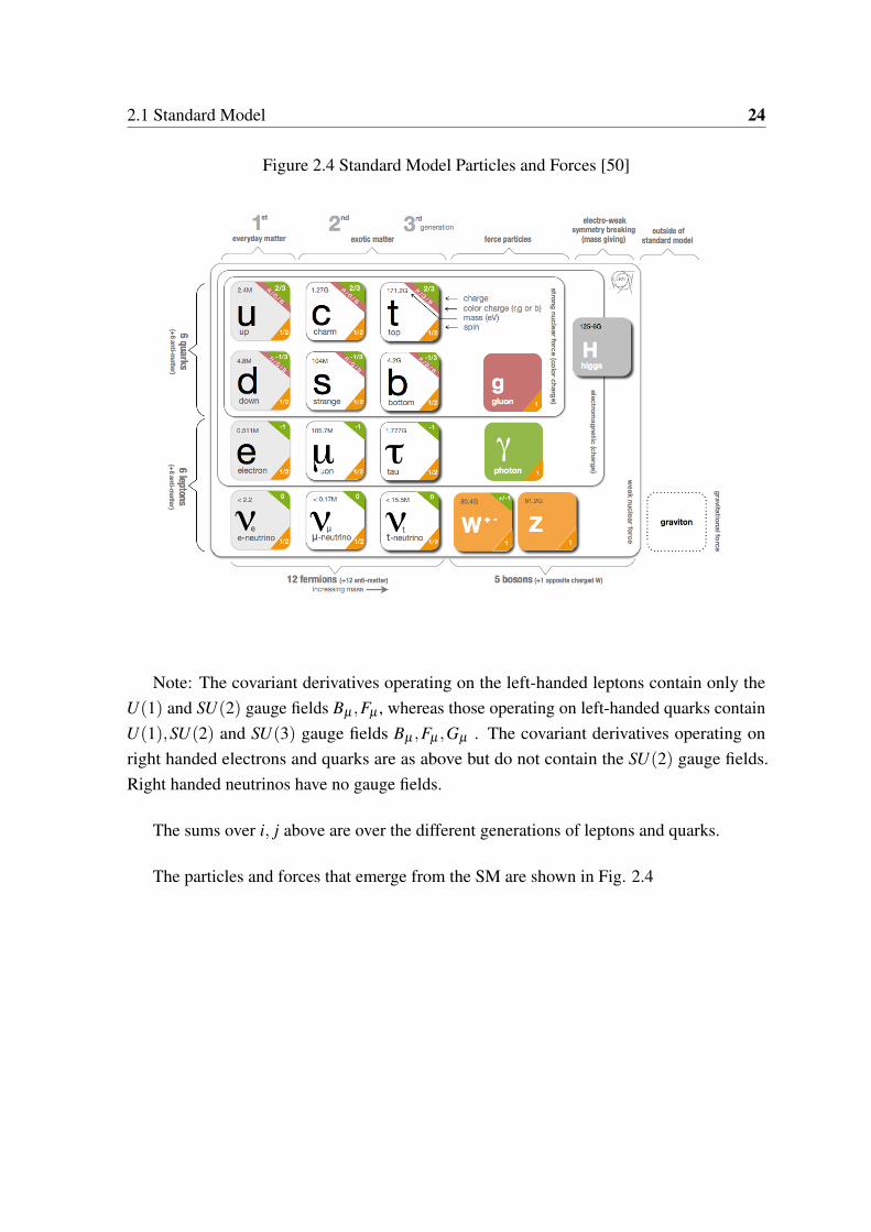
Figure 24 Standard Model Particles and Forces [50]
Note The covariant derivatives operating on the left-handed leptons contain only theU(1) and SU(2) gauge fields Bmicro Fmicro whereas those operating on left-handed quarks containU(1)SU(2) and SU(3) gauge fields Bmicro Fmicro Gmicro The covariant derivatives operating onright handed electrons and quarks are as above but do not contain the SU(2) gauge fieldsRight handed neutrinos have no gauge fields
The sums over i j above are over the different generations of leptons and quarks
The particles and forces that emerge from the SM are shown in Fig 24
22 Dark Matter 25
22 Dark Matter
221 Evidence for the existence of dark matter
2211 Bullet Cluster of galaxies
Most of the mass of the cluster as measured by a gravitational lensing map is concentratedaway from the centre of the object The visible matter (as measured by X-ray emission) ismostly present in the centre of the object The interpretation is that the two galaxy clustershave collided perpendicular to the line of sight with the mostly collisionless dark matterpassing straight through and the visible matter interacting and being trapped in the middleIt was estimated that the ratio of actual to visible matter was about 16 [51]
Figure 25 Bullet Cluster [52]
2212 Coma Cluster
The first evidence for dark matter came in the 1930s when Fritz Zwicky observed the Comacluster of galaxies over 1000 galaxies gravitationally bound to one another He observed thevelocities of individual galaxies in the cluster and estimated the amount of matter based onthe average galaxy He calculated that many of the galaxies should be able to escape fromthe cluster unless the mass was about 10 times higher than estimated
22 Dark Matter 26
2213 Rotation Curves [53]
Since those early observations many spiral galaxies have been observed with the rotationcurves calculated by doppler shift with the result that in all cases the outermost stars arerotating at rates fast enough to escape their host galaxies Indeed the rotation curves arealmost flat indicating large amounts of dark matter rotating with the galaxies and holdingthe galaxies together
Figure 26 Galaxy Rotation Curves [54]
2214 WIMPS MACHOS
The question is if the particles that make up most of the mass of the universe are not baryonswhat are they It is clear that the matter does not interact significantly with radiation so mustbe electrically neutral It has also not lost much of its kinetic energy sufficiently to relax intothe disks of galaxies like ordinary matter Massive particles may survive to the present ifthey carry a conserved additive or multiplicative quantum number This is so even if equalnumbers of particles and anti-particles can annihilate if the number densities become too lowto reduce the density further These particles have been dubbed Weakly interacting MassiveParticles (WIMPS) as they interact with ordinary matter only through a coupling strengthtypically encountered in the weak interaction They are predicted to have frozen out ofthe hot plasma and would give the correct relic density based solely on the weak interactioncross section (sometimes called the WIMP Miracle) Another possibility called MassiveCompact Halo Objects (MACHOS)- are brown dwarf stars Jupiter mass objects or remnantsfrom an earlier generation of star formation
22 Dark Matter 27
2215 MACHO Collaboration [55]
In order to estimate the mass of MACHOS a number of experiments have been conductedusing microlensing which makes use of the fact that if a massive object lies in the line ofsight of a much more distant star the light from the more distant star will be lensed and forma ring around the star It is extemely unlikely that the MACHO will pass directly through theline of sight but if there is a near miss the two images will be seperated by a small angleThe signature for microlensing is a time-symmetric brightening of a star as the MACHOpasses near the line of sight called a light curve One can obtain statistical information aboutthe MACHO masses from the shape and duration of the light curves and a large number ofstars (many million) must be monitored The MACHO Collaboration [55] have monitoredover 11 million stars and less than 20 events were detected The conclusion was that thiscould account for a small addition (perhaps up to 20 ) to the visible mass but not enoughto account for Dark Matter
2216 Big Bang Nucleosynthesis (BBN) [56]
Another source of evidence for DM comes from the theory of Nucleosynthesis in the fewseconds after the Big Bang In the first few minutes after the big bang the temperatures wereso high that all matter was dissociated but after about 3 minutes the temperature rapidlycooled to about 109 Kelvin Nucleosynthesis could begin when protons and neutrons couldstick together to form Deuterium (Heavy Hydrogen) and isotopes of Helium The ratio ofDeuterium to Hydrogen and Helium is very much a function of the baryon density and alsothe rate of expansion of the universe at the time of Nucleosynthesis There is a small windowwhen the density of Baryons is sufficient to account for the ratios of the various elementsThe rate of expansion of the universe is also a function of the total matter density The ratiosof these lighter elements have been calculated by spectral measurements with Helium some25 of the mass of the universe Deuterium 001 The theory of BBN accounts for theratios of all of the lighter elements if the ratio of Baryon mass to total mass is a few percentsuggesting that the missing matter is some exotic non-baryonic form
22 Dark Matter 28
2217 Cosmic Microwave Background [57]
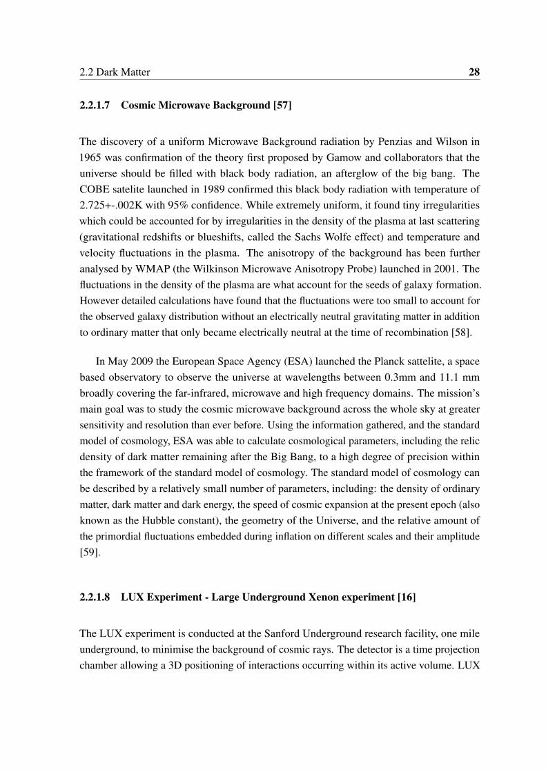
The discovery of a uniform Microwave Background radiation by Penzias and Wilson in1965 was confirmation of the theory first proposed by Gamow and collaborators that theuniverse should be filled with black body radiation an afterglow of the big bang TheCOBE satelite launched in 1989 confirmed this black body radiation with temperature of2725+-002K with 95 confidence While extremely uniform it found tiny irregularitieswhich could be accounted for by irregularities in the density of the plasma at last scattering(gravitational redshifts or blueshifts called the Sachs Wolfe effect) and temperature andvelocity fluctuations in the plasma The anisotropy of the background has been furtheranalysed by WMAP (the Wilkinson Microwave Anisotropy Probe) launched in 2001 Thefluctuations in the density of the plasma are what account for the seeds of galaxy formationHowever detailed calculations have found that the fluctuations were too small to account forthe observed galaxy distribution without an electrically neutral gravitating matter in additionto ordinary matter that only became electrically neutral at the time of recombination [58]
In May 2009 the European Space Agency (ESA) launched the Planck sattelite a spacebased observatory to observe the universe at wavelengths between 03mm and 111 mmbroadly covering the far-infrared microwave and high frequency domains The missionrsquosmain goal was to study the cosmic microwave background across the whole sky at greatersensitivity and resolution than ever before Using the information gathered and the standardmodel of cosmology ESA was able to calculate cosmological parameters including the relicdensity of dark matter remaining after the Big Bang to a high degree of precision withinthe framework of the standard model of cosmology The standard model of cosmology canbe described by a relatively small number of parameters including the density of ordinarymatter dark matter and dark energy the speed of cosmic expansion at the present epoch (alsoknown as the Hubble constant) the geometry of the Universe and the relative amount ofthe primordial fluctuations embedded during inflation on different scales and their amplitude[59]
2218 LUX Experiment - Large Underground Xenon experiment [16]
The LUX experiment is conducted at the Sanford Underground research facility one mileunderground to minimise the background of cosmic rays The detector is a time projectionchamber allowing a 3D positioning of interactions occurring within its active volume LUX
22 Dark Matter 29
Figure 27 WMAP Cosmic Microwave Background Fluctuations [58]
Figure 28 Dark Matter Interactions [60]
uses as its target 368 kiliograms of liquefied ultra pure xenon which is a scintillator Interac-tions inside the xenon will create an amount of light proportional to the energy depositedThat light can be collected on arrays of light detectors sensitive to a single photon
Xenon is very pure and the amount of radiation originating within the target is limitedAlso being three times denser than water it can stop radiation originating from outside thedetector The 3D detector focuses on interactions near the center which is a quiet regionwhere rare dark matter interactions might be detected [16]
22 Dark Matter 30
222 Searches for dark matter
2221 Dark Matter Detection
Fig 28 illustrates the reactions studied under the different forms of experiment designed todetect DM
Direct detection experiments are mainly underground experiments with huge detectorsattempting to detect the recoil of dark matter off ordinary matter such as LUX [16] CDMS-II [61] XENON100 [11] COUPP [62] PICASSO [63] ZEPLIN [10] These involveinteractions between DM and SM particles with final states involving DM and SM particles
Indirect detection involves the search for the annihilation of DM particles in distantastrophysical sources where the DM content is expected to be large Example facilitiesinclude space based experiments (EGRET [64] PAMELA [18] FERMI-LAT [65]) balloonflights (ATIC [66] PEBS [67] PPB-BETS [68]) or atmospheric Cherenkov telescopes(HESS [69]MAGIC [70]) and neutrino telescopes (SuperKamiokande [71] IceCube [72]ANTARES [73] KM3NET [74]) Indirect Detection involves DM particles in the initial stateand SM particles in the final state
Collider detection involves SM particles in the initial state creating DM particles in thefinal state which can be detected by missing transverse energy and explained by variousmodels extending the SM
223 Possible signals of dark matter
224 Gamma Ray Excess at the Centre of the Galaxy [65]
The center of the galaxy is the most dense and active region and it is no surprise that itproduces intense gamma ray sources When astronomers subtract all known gamma raysources there remains an excess which extends out some 5000 light years from the centerHooper et al find that the annihilation of dark matter particles with a mass between 31 and40 Gev fits the excess to a remarkable degree based on Gamma Ray spectrum distributionand brightness
23 Background on ATLAS and CMS Experiments at the Large Hadron collider (LHC) 31
Figure 29 Gamma Ray Excess from the Milky Way Center [75]
23 Background on ATLAS and CMS Experiments at theLarge Hadron collider (LHC)
The collider constraints in this paper are based on two of the experiments that are part of theLHC in CERN
Figure 210 ATLAS Experiment
The LHC accelerates proton beams in opposite directions around a 27 km ring of super-conducting magnets until they are made to collide at an interaction point inside one of the 4experiments placed in the ring An upgrade to the LHC has just been performed providing65 TeV per beam
23 Background on ATLAS and CMS Experiments at the Large Hadron collider (LHC) 32
231 ATLAS Experiment
The ATLAS detector consists of concentric cylinders around the interaction point whichmeasure different aspects of the particles that are flung out of the collision point There are 4major parts the Inner Detector the Calorimeters the Muon spectrometer and the magnetsystems
2311 Inner Detector
The inner detector extends from a few centimeters to 12 meters from the interaction point andmeasures details of the charged particles and their momentum interacting with the materialIf particles seem to originate from a point other than the interaction point this may indicatethat the particle comes from the decay of a hadron with a bottom quark This is used to b-tagcertain particles
The inner detector consists of a pixel detector with three concentric layers and threeendcaps containing detecting silicon modules 250 microm thick The pixel detector has over 80million readout channels about 50 percent of the total channels for the experiment All thecomponents are radiation hardened to cope with the extremely high radiation in the proximityof the interaction point
The next layer is the semi-conductor layer (SCT) similar in concept to the pixel detectorbut with long narrow strips instead of pixels to cover a larger area It has 4 double layers ofsilicon strips with 63 million readout channels
The outermost component of the inner detector is the Transition Radiation Tracker It is acombination of a straw tracker and a transition radiation detector The detecting elementsare drift tubes (straws) each 4mm in diameter and up to 144 cm long Each straw is filledwith gas which becomes ionised when the radiation passes through The straws are held at-1500V with a thin wire down the center This drives negatively ionised atoms to the centercausing a pulse of electricity in the wire This causes a pattern of hit straws allowing the pathof the particles to be determined Between the straws materials with widely varying indicesof refraction cause transition radiation when particles pass through leaving much strongersignals in some straws Transition radiation is strongest for highly relativistic particles (thelightest particles- electrons and positrons) allowing strong signals to be associated with theseparticles
23 Background on ATLAS and CMS Experiments at the Large Hadron collider (LHC) 33
2312 Calorimeters
The inner detector is surrounded by a solenoidal magnet of 2 Tesla (there is also an outertoroidal magnet) but surrounding the inner magnet are the calorimeters to measure theenergy of particles by absorbing them There is an inner electromagnetic calorimeter whichmeasures the angle between the detectorrsquos beam axis and the particle (or more preciselypseudo-rapidity) and its angle in the perpendicular plane to a high degree of accuracy Theabsorbing material is lead and stainless steel and the sampling material liquid argon Thehadron calorimeter measures the energy of particles that interact via the strong force Theenergy absorbing material is scintillating steel
2313 Muon Specrometer
The muon spectrometer surrounds the calorimeters and has a set of 1200 chambers tomeasure the tracks of outgoing muons with high precision using a magnetic field andtriggering chambers Very few particles of other types pass through the calorimeters and aresubsequently measured
2314 Magnets
The magnets are in two layers the inner solenoidal and outer toroidal which together causecharged particles to curve in the magetic field allowing their momentum to be determinedThe outer toroidal magnet consists of 8 very large air core superconducting magnets whichsupply the field in the muon spectrometer
232 CMS Experiment
The CMS Detector is similar in design to the ATLAS Detector with a single solenoidalmagnet which is the largest of its type ever built (length 13m and diameter 7m) and allowsthe tracker and calorimeter detectors to be placed inside the coil in a compact way Thestrong magnetic field gives a high resolution for measuring muons electrons and photons ahigh quality central tracking system and a hermetic hadron calorimeter designed to preventhadrons from escaping
23 Background on ATLAS and CMS Experiments at the Large Hadron collider (LHC) 34
Figure 211 CMS Experiment
Chapter 3
Fitting Models to the Observables
31 Simplified Models Considered
In order to extend the findings of previous studies [19] to include collider constraints wefirst performed Bayesian scans [7] over three simplified models real scalar dark matter φ Majorana fermion χ and real vector Xmicro The purpose was to obtain the most probable regionsof each model then to use the resulting posterior samples to investigate whether the LHCexperiments have any sensitivity to the preferred regions
The three models couple to the mediator with interactions shown in the following table
Table 31 Simplified Models
Hypothesis real scalar DM Majorana fermion DM real vector DM
DM mediator int Lφ sup microφ mφ φ 2S Lχ sup iλχ
2 χγ5χS LX sup microX mX2 X microXmicroS
The interactions between the mediator and the standard fermions is assumed to be
LS sup f f S (31)
and in line with minimal flavour violation we only consider third generation fermions- ief = b tτ
For the purposes of these scans we consider the following observables
32 Observables 36
32 Observables
321 Dark Matter Abundance
We have assumed a single dark matter candidate which freezes out in the early universe witha central value as determined by Planck [21] of
ΩDMh2 = 01199plusmn 0031 (32)
h is the reduced hubble constant
The experimental uncertainty of the background relic density [59] is dominated by atheoretical uncertainty of 50 of the value of the scanned Ωh2 [76] We have added thetheoretical and the experimental uncertainties in quadrature
SD =radic(05Ωh2)2 + 00312 (33)
This gives a log likelihood of
minus05lowast (Ωh2 minus 1199)2
SD2 minus log(radic
2πSD) (34)
322 Gamma Rays from the Galactic Center
Assuming that the gamma ray flux excess from the galactic centre observed by Fermi-LAT iscaused by self annihilation of dark matter particles the differential flux
d2Φ
dEdΩ=
lt σv gt8πmχ
2 J(ψ)sumf
B fdN f
γ
dE(35)
has been calculated using both Micromegas v425 with a Navarro-Frenk-White (NFW) darkmatter galactic distribution function
ρ(r) = ρ0(rrs)
minusγ
(1+ rrs)3minusγ (36)
with γ = 126 and an angle of 5 to the galactic centre [19]
32 Observables 37
Here Φ is the flux dE is the differential energy lt σv gt the velocity averaged annihi-lation cross section of the dark matter across the galactic centre mχ the mass of the darkmatter particle B f =lt σv gt f σv is the annihilation fraction into the f f final state anddN f
γ dE is the energy distribution of photons produced in the annihilation channel with thefinal state f f The J factor is described below
The angle ψ to the galactic centre determines the normalisation of the gamma ray fluxthrough the factor
J(ψ) =int
losρ(l2 + r⊙2 minus2lr⊙cosψ)dl (37)
where ρ(r) is the dark matter density at distance r from the centre of the galaxy r⊙=85 kpcis the solar distance from the Galactic center ρ0 is set to reproduce local dark matter densityof 03GeVcm3
The central values for the gamma ray spectrum were taken from Fig 5 of [77] and thestandard deviations of individual flux points from the error bars on the graph In commonwith [78] we ignore possible segment to segment correlations
For the Fermi-LAT log likelihood we assumed each point was distributed with indepen-dent Gaussian likelihood with the experimental error for each data point given by the errorbar presented in Fig5 of [76] for each point We also assumed an equal theoretical errorfor each point which when added to the experimental error in quadrature gave an effectivelog likelihood for each point of minus05lowast (giminusdi)
2
2lowastσ2i
where gi are the calculated values and di theexperimental values and σi the experimental errors
323 Direct Detection - LUX
The LUX experiment [16] is the most constraining direct search experiment to date for awide range of WIMP models We have used LUXCalc [79] (modified to handle momentumdependent nucleon cross sections) to calculate the likelihood of the expected number ofsignal events for the Majorana fermion model
The likelihood function is taken as the Poisson distribution
L(mχ σ | N) = P(N | mχ σ) =(b+micro)Neminus(b+micro)
N (38)
32 Observables 38
where b= expected background of 064 and micro = micro(mχσ ) is the expected number of signalevents calculated for a given model
micro = MTint
infin
0dEφ(E)
dRdE
(E) (39)
where MT is the detector mass times time exposure and φ(E) is a global efficiency factorincorporating trigger efficiencies energy resolution and analysis cuts
The differential recoil rate of dark matter on nucleii as a function of recoil energy E
dRdE
=ρX
mχmA
intdvv f (v)
dσASI
dER (310)
where mA is the nucleon mass f (v) is the dark matter velocity distribution and
dσSIA
dER= Gχ(q2)
4micro2A
Emaxπ[Z f χ
p +(AminusZ) f χn ]
2F2A (q) (311)
where Emax = 2micro2Av2mA Gχ(q2) = q2
4m2χ
[24] is an adjustment for a momentum dependantcross section which applies only to the Majorana model
f χ
N =λχ
2m2SgSNN assuming that the relic density is the central value of 1199 We have
implemented a scaling of the direct search cross section in our code by multiplying gSNN by( Ω
Ω0)05 as a convenient method of allowing for the fact that the actual relic density enters
into the calculation of the cross section as a square
FA(q) is the nucleus form factor and
microA =mχmA
(mχ +mA)(312)
is the reduced WIMP-nucleon mass
The strength of the dark matter nucleon interaction between dark matter particles andthird generation quarks is
gSNN =2
27mN fT G sum
f=bt
λ f
m f (313)
where fT G = 1minus f NTuminus f N
Tdminus fTs and f N
Tu= 02 f N
Td= 026 fTs = 043 [20]
33 Calculations 39
For the real scalar and real vector models where the spin independent cross sections arenot momentum dependent we based the likelihood on the LUX 95 CL from [16] using acomplementary error function Li(d|mχ I) = 05lowastCEr f (dminusx(mχ )
σ) where x is the LUX limit
and d the calculated SI cross section We assumed a LUX error σ of 01lowastd lowastradic
2
33 Calculations
We coded the Lagrangians for the three models in Feynrules [4] Calculation of the expectedobservables (dark matter relic density Fermi-LAT gamma ray spectrum and LUX nucleonscattering amplitudes) were performed using Micromegas v425
331 Mediator Decay
A number of searches have previously been performed at the LHC which show sensitivity tothe decay of scalar mediators in the form of Higgs bosons (in beyond the standard modeltheories) to bottom quarks top quarks and τ leptons (all third generation fermions) Two inparticular [43 44] provide limits on the cross-sections for the production of the scalar timesthe branching ratios to brsquos and τrsquos In order to check these limits against each of the modelswe ran parameter scans in Madgraph at leading order over the top 900 points from the nestedsampling output from MultiNest [19]
The two processes were
1) To compare with the limits in Search for neutral MSSM Higgs bosons decaying to apair of τ leptons in pp collisions [44]
bull generate p p gt b b S where S is the scalar mediator
The process measures the decay of a scalar in the presence of b-jets that decay to τ+τminus
leptons Fig31 shows the main diagrams contributing to the process The leftmost diagramis a loop process and the centre and right are tree level however we only got Madgraph togenerated the middle diagram since we are interested in τ leptons and b quarks in the finalstate
The limit given in [44] only applies in the case of narrow resonances where narrow istaken to mean that the width of the resonance is less than 10 of its mass To test the validity
33 Calculations 40
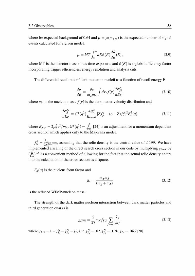
Figure 31 Main Feyman diagrams leading to the cross section for scalar decaying to a pairof τ leptons
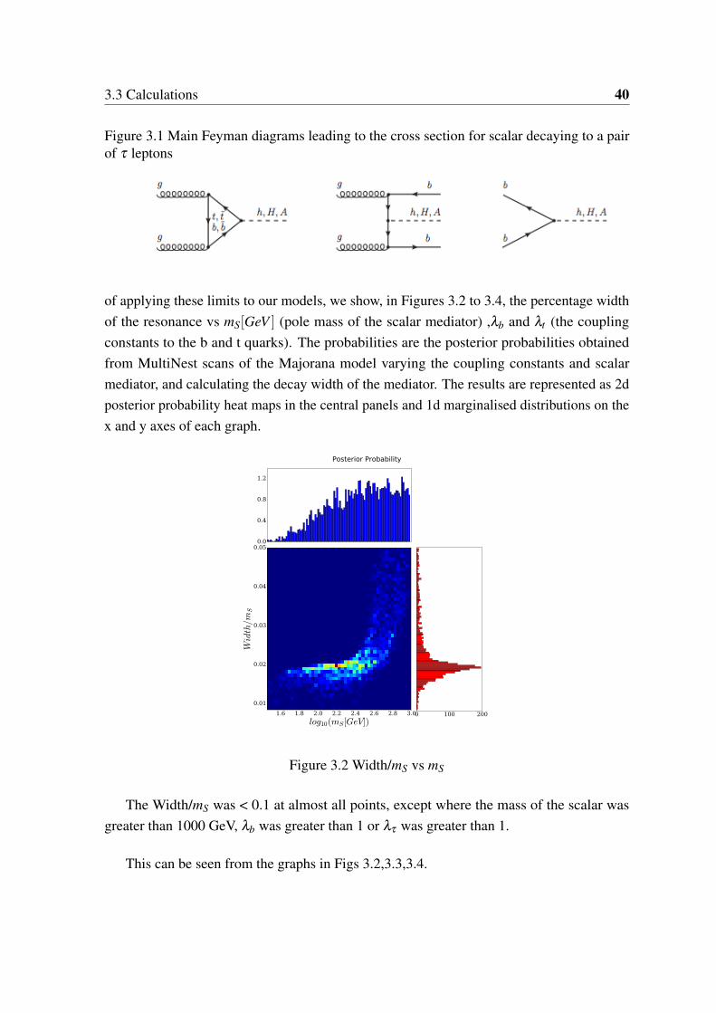
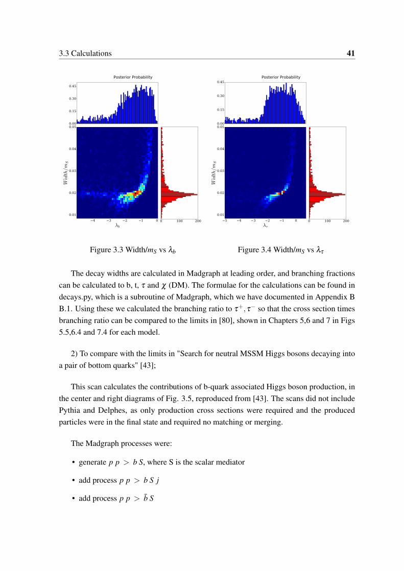
of applying these limits to our models we show in Figures 32 to 34 the percentage widthof the resonance vs mS[GeV ] (pole mass of the scalar mediator) λb and λt (the couplingconstants to the b and t quarks) The probabilities are the posterior probabilities obtainedfrom MultiNest scans of the Majorana model varying the coupling constants and scalarmediator and calculating the decay width of the mediator The results are represented as 2dposterior probability heat maps in the central panels and 1d marginalised distributions on thex and y axes of each graph
16 18 20 22 24 26 28 30
log10(mS[GeV])
001
002
003
004
005
Widthm
S
00
04
08
12
0 100 200
Posterior Probability
Figure 32 WidthmS vs mS
The WidthmS was lt 01 at almost all points except where the mass of the scalar wasgreater than 1000 GeV λb was greater than 1 or λτ was greater than 1
This can be seen from the graphs in Figs 323334
33 Calculations 41
4 3 2 1 0
λb
001
002
003
004
005
WidthmS
000
015
030
045
0 100 200
Posterior Probability
Figure 33 WidthmS vs λb
5 4 3 2 1 0
λτ
001
002
003
004
005
WidthmS
000
015
030
045
0 100 200
Posterior Probability
Figure 34 WidthmS vs λτ
The decay widths are calculated in Madgraph at leading order and branching fractionscan be calculated to b t τ and χ (DM) The formulae for the calculations can be found indecayspy which is a subroutine of Madgraph which we have documented in Appendix BB1 Using these we calculated the branching ratio to τ+τminus so that the cross section timesbranching ratio can be compared to the limits in [80] shown in Chapters 56 and 7 in Figs5564 and 74 for each model
2) To compare with the limits in Search for neutral MSSM Higgs bosons decaying intoa pair of bottom quarks [43]
This scan calculates the contributions of b-quark associated Higgs boson production inthe center and right diagrams of Fig 35 reproduced from [43] The scans did not includePythia and Delphes as only production cross sections were required and the producedparticles were in the final state and required no matching or merging
The Madgraph processes were
bull generate p p gt b S where S is the scalar mediator
bull add process p p gt b S j
bull add process p p gt b S
33 Calculations 42
Figure 35 Main Feyman diagrams leading to the cross section for scalar decaying to a pairof b quarks in the presence of at least one b quark
bull add process p p gt b S j
The cross section times branching ratios to bb for mediator production in association withat least one b quark is shown for each model in Chapters 56 and 7 in Figs 5765 and 75
332 Collider Cuts Analyses
We generated two parameter scans with parameter combinations from the Multinest outputwhich were the basis of the plots of Fig 6 in [19] The plots in Fig 6 were marginalisedto two parameters each but the raw Multinest output contained 5 parameters plus the priorprobabilities of each combination normalised to total 10
The first scan was for χ produced with b quarks In order to force the mediator to decayto χ only we had χ in the final state and defined jets to include b quarks in Madgraph Thenwe generated the processes
bull generate p p gt χ χ j
bull add process p p gt χ χ j j
Jet matching was on
The second scan was for t quarks produced in the final state
bull generate p p gt χ χ tt
33 Calculations 43
No jet matching was required because we did not mix final state jet multiplicities at thematrix element level
The outputs from these two processes were normalised to 21 f bminus1 and combined
The results of these scans prior to collider cuts calculations are shown in Figs 5161and 71 These show the posterior probabilities of the various parameter combinations withdifferent constraints applied seperately and then together A more detailed commentary isgiven in each of the sections
We then sampled 900 points based on posterior probability from these scans and ran thesethrough Madgraph v425 then applied collider cuts with the C++ code using the limits fromthe following six ATLAS and CMS searches shown in Table32 and described below to findany exclusions
333 Description of Collider Cuts Analyses
In the following all masses and energies are in GeV and angles in radians unless specificallystated
3331 Lepstop0
Search for direct pair production of the top squark in all-hadronic final states in pro-tonndashproton collisions at
radics=8 TeV with the ATLAS detector[32]
This analysis searched for direct pair production of the supersymmetric partner to thetop quark using integrated luminosity of 201 f bminus1 The top squark was assumed to de-cay via t rarr t χ0
1 or t rarr bχ01 or t rarr bχ
plusmn1 rarr bW (lowast)χ1
0 where χ01 (χ
plusmn1 ) denotes the lightest
neutralino(chargino) in supersymmetric models The search targets a fully hadronic finalstate with four or more jets and large missing momentum The production of a mediator inassociation with top quarks followed by an invisible mediator decay to dark matter particleshas a similar final state to that considered in the ATLAS stop searches Thus we expect theATLAS reach to have sensitivity to the three dark matter models considered in this thesis
The collider cuts program mimicked the object reconstruction through jetlepton overlapremoval and selected signal electrons muons and τ particles with pT gt 10 GeV and
33 Calculations 44
Table 32 95 CL by Signal Region
Experiment Region Number
Lepstop0
SRA1 66SRA2 57SRA3 67SRA4 65SRC1 157SRC2 124SRC3 80
Lepstop1
SRtN1-1 857SRtN1-2 498SRtN1-3 389SRtN2 107SRtN3 85SRbC1 832SRbC2 195SRbC3 76
Lepstop2
L90 740L100 56L110 90L120 170
2bstop
SRA 857SRB 270SRA150 380SRA200 260SRA250 90SRA300 75SRA350 52
CMSTopDM1L SRA 1385
ATLASMonobjetSR1 1240SR2 790
33 Calculations 45
|η | lt 24724 and 247 respectively (for eminusmicrominusτ) Jets were selected with pT gt 20 GeVand |η |lt 45 b-jets were selected if they were tagged by random selection lt 70 and had|η |lt 25 and pT gt 20 GeV
These jets and leptons were further managed for overlap removal within ∆R lt 04 withnon b-jets removed if ∆R lt 02
The b-jets and non b-jets were further selected as signal jets if pT gt 35 GeV and |η |lt 28
These signal jets electrons and muons were finally binned according to the signal regionsin Tables 333435 below
Table 33 Selection criteria common to all signal regions
Trigger EmissT
Nlep 0b-tagged jets ⩾ 2
EmissT 150 GeV
|∆φ( jet pmissT )| gtπ5
mbminT gt175 GeV
Table 34 Selection criteria for signal regions A
SRA1 SRA2 SRA3 SRA4anti-kt R=04 jets ⩾ 6 pT gt 808035353535 GeV
m0b j j lt 225 GeV [50250] GeV
m1b j j lt 225 GeV [50400] GeV
min( jet i pmissT ) - gt50 GeV
τ veto yesEmiss
T gt150 GeV gt250 GeV gt300 GeV gt 350 GeV
Table 35 Selection criteria for signal regions C
SRC1 SRC2 SRC3anti-kt R=04 jets ⩾ 5 pT gt 8080353535 GeV
|∆φ(bb)| gt02 π
mbminT gt185 GeV gt200 GeV gt200 GeV
mbmaxT gt205 GeV gt290 GeV gt325 GeV
τ veto yesEmiss
T gt160 GeV gt160 GeV gt215 GeV
wherembmin
T =radic
2pbt Emiss
T [1minus cos∆φ(pbT pmiss
T )]gt 175 (314)
33 Calculations 46
and pbT is calculated for the b-tagged jet with the smallest ∆φ to the pmiss
T direction andmbmax
T is calculated with the pbT for the b-tagged jet with the largest ∆φ to the pmiss
T direction
m0b j j is obtained by first selecting the two jets with the highest b-tagging weight- from
the remaining jets the two jets closest in the η minusφ plane are combined to form a W bosoncandidate this candidate is then combined with the closest of the 2 b-tagged jets in the η minusφ
plane to form the first top candidate with mass m0b j j A second W boson candidate is formed
by repeating the procedure with the remaining jets this candidate is combined with thesecond of the selected b-tagged jets to form the second top candidate with mass m1
b j j Thecuts shown in Appendix1 Table A1 show the cumulative effect of the individual cuts appliedto the data the signal region cuts and the cumulative effects of individual cuts in SignalRegion C
3332 Lepstop1
Search for direct top squark pair production in final states with one isolated leptonjets and missing transverse momentum in
radics=8 TeV pp collisions using 21 f bminus1 of
ATLAS data[33]
The stop decay modes considered were those to a top quark and the lightest supersym-metric particle (LSP) as well as a bottom quark and the lightest chargino where the charginodecays to the LSP by emitting a W boson We should expect the three dark matter models inthis paper with couplings to t and b quarks to show some visibility in this search
The collider cuts program mimicked the object construction by selecting electrons andmuons with pT gt 10 GeV and |η |lt 247 and 24 respectively and jets with pT gt 20 GeVand |η |lt 10 b-jets with |η |lt 25 and pT gt 25 GeV were selected with random efficiency75 and mistag rate 2 (where non b-jets were mis-classified) We then removed any jetwithin ∆R = 02 of an electron and non overlapping jets with |η |lt 28 were used to removeany electrons and muons within ∆R = 04 of these while non-overlapping jets with |η |lt 25and pT gt 25 GeV were classified as signal jets Non overlapping electrons and muons withpT gt 25 GeV were classified as signal electrons and muons
Signal selection defined six regions to optimize sensitivity for different stop and LSPmasses as well as sensitivity to two considered stop decay scenarios Three signal regionslabelled SRbC 1-3 where bC is a moniker for b+Chargino and 3 regions labelled SRtN 1-3where tN is a moniker for t+Neutralino were optimised for the scenarios where t1 decaysto the respective particles indicated by the labels Increasing label numbers correspond toincreasingly strict selection criteria
33 Calculations 47
The dominant background in all signal regions arises from dileptonic tt events All threeSRtN selectons impose a requirement on the 3-jet mass m j j j of the hadronically decayingtop quark to specifically reject the tt background where both W bosons from the top quarkdecay leponically
For increasing stop mass and increasing difference between the stop and the LSP therequirents are tightened on Emiss
T on the ratio EmissT
radicHT where HT is the scalar sum of the
momenta of the four selected jets and also tightened on mT
To further reduce the dileptonic tt background for an event characterised by two one stepdecay chains a and b each producing a missing particle C use is made of the variable
mT 2 =min
pCTa + pC
T b = pmissT
[max(mTamtb)] (315)
where mTi is the transverse mass 1 of branch i for a given hypothetical allocation (pCTa pC
T b)
of the missing particle momenta Eqn 315 is extended for more general decay chains byamT 2 [81] which is an asymmetric form of mT 2 in which the missing particle is the W bosonin the branch for the lost lepton and the neutrino is the missing particle for the branch withthe observed charged lepton
∆φ( jet12 pmissT ) the azimuthal angle between leading or subleading jets and missing mo-
mentum is used to suppress the background from mostly multijet events with mis-measuredEmiss
T
Events with four or more jets are selected where the jets must satisfy |η | lt 25 and pT gt80604025 GeV respectively
These signal particles were then classified according to the cutflows analysis in Fig36below and compared with the paper in Appendix1 Table A2
3333 Lepstop2
Search for direct top squark pair production in final states with two leptons in p pcollisions at
radics=8TeV with the ATLAS detector[34]
Three different analysis strategies are used to search for t1 pair production Two targett1 rarr b+ χ
plusmn1 decay and the three body t1 rarr bW χ0
1 decay via an off-shell top quark whilst
1The transverse mass is defined as m2T = 2plep
T EmissT (1minus cos(∆φ)) of branch i where ∆φ is the azimuthal
angle between the lepton and the missing transverse momentum
33 Calculations 48
Table 36 Signal Regions - Lepstop1
Requirement SRtN2 SRtN3 SRbC1 SRbC2 SRbC3∆φ( jet1 pmiss
t )gt - 08 08 08 08∆φ( jet2 pmiss
T )gt 08 08 08 08 08Emiss
T [GeV ]gt 200 275 150 160 160Emiss
T radic
HT [GeV12 ]gt 13 11 7 8 8
mT [GeV ]gt 140 200 120 120 120me f f [GeV ]gt - - - 550 700amT 2[GeV ]gt 170 175 - 175 200mT
T 2[GeV ]gt - 80 - - -m j j j Yes Yes - - -
one targets t1 rarr t + χ01 to an on shell quark decay mode The analysis is arranged to look
at complementary mass splittings between χplusmn1 and χ0
1 smaller and larger than the W bosonmass The smaller splitting provides sensitivity to t1 three body decay
Object reconstruction was carried out by selecting baseline electronsmuons and τrsquos withpT gt 10 GeV and |η |lt 24724 and 247 respectively Baseline jets and b-jets were selectedwith pT gt 20 GeV and |η |lt 25 and b-jets with 70 efficiency Baseline jets were removedif within ∆R lt 02 of an electron and electrons and muons were removed if within ∆R lt 04of surviving jets Signal electrons required pT gt 10 GeV and signal jets pT gt 20 GeV and|η |lt 25
The analysis made use of the variable mT 2 [82] the stransverse mass used to mea-sure the masses of pair-produced semi-invisibly decaying heavy particles It is definedas mT 2(pT1 pT2qT ) =
minqT1+qT2=qT
max[mT (pT1qT1)mT (pT2qT2)] where mT indicatesthe transverse mass pT1 and pT2 are vectors and qT = qT1 + qT2 The minimisation isperformed over all possible decompositions of qT
Events were selected if they passed either a single-electron a single-muon a double-electron a double-muon or an electron-muon trigger Events are required to have exactlytwo opposite sign leptons and at least one of the leptons or muons must have a momentumgreater than 25 GeV and the invariant mass (rest mass) of the two leptons is required to begreater than 20 GeV In order to reduce the number of background events containing twoleptons produced by the on-shell decay of the Z boson the invariant mas must be outside711-111 GeV range
Two additional selections are applied to reduce the number of background events withhigh mT 2 arising from events with large Emiss
T due to mismeasured jets ∆φb lt 15 and∆φ gt 10 The quantity ∆φb is the azimuthal angle between pll
T b = pmissT + pl1
T +Pl2T The
33 Calculations 49
vector pllT b is the opposite of the vector sum of all the hadronic activity in the event For WW
and tt backgrounds it measures the transverse boost of the WW system and for the signalthe transverse boost of the chargino-chargino system The ∆φ variable is the azimuthal anglebetween the pmiss
T vector and the direction of the closest jet
By requiring mT 2 gt 40 GeV the tt background is the dominant background in both thesame-flavoured (SF) and different-flavoured (DF) events
Four signal regions are then defined as shown in Table 37 SR M90 has the loosestselection requiring MT 2gt 90 GeV and no additional requirement on jets and providessensitivity to scenarios with a small difference between the masses of the top-squark andchargino SR M110 and M120 have a loose selection on jets requiring two jets with pT
gt 20 GeV and mT 2 to be greater than 110 GeV and 120 GeV respectively They providesensitivity to scenarios with small to moderate difference between the invariant masses of thestop quark and the charginos SR M100 has a tighter jet slection and provides sensitivity toscenarios with a large mass difference between the both stop quark and the chargino and thestop quark and the neutralino
The analysis cut regions are summarised in Fig37 below
Table 37 Signal Regions Lepstop2
SR M90 M100 M110 M120pT leading lepton gt 25 GeV
∆φ(pmissT closest jet) gt10
∆φ(pmissT pll
T b) lt15mT 2 gt90 GeV gt100 GeV gt110 GeV gt120 GeV
pT leading jet no selection gt100 GeV gt20 GeV gt20 GeVpT second jet no selection gt50 GeV gt20 GeV gt20 GeV
To validate the code we ran the cuts shown in Appendix 1 Table A3 with the givenMadgraph simulation and compared to [83] It was not clear what baseline cuts had beenemployed in the ATLAS paper so our results were normalised to the 2 SF electrons beforecomparison Some of the ATLAS cut numbers were less than 3 and we did not produce anyevents passing these cuts but clearly the margin of error at this level was greater than thenumber of ATLAS events
33 Calculations 50
3334 2bstop
Search for direct third-generation squark pair production in final states with miss-ing transverse momentum and two b-jets in
radics= 8 TeV pp collisions with the ATLAS
detector[31]
Two sets of scenarios are considered In the first the coloured sbottom is the onlyproduction process decaying via b1 rarr bχ0
1 In the second the stop is the only productionprocess decaying via t1 rarr t χplusmn
1 and the lightest chargino (χplusmn1 ) decays via a virtual W boson
into the final state χ01 f f prime Both scenarios are characterised by the presence of two jets
resulting from the hadronisation of b quarks and large missing transverse momentum Theproduction of a mediator in association with top quarks followed by an invisible mediatordecay to dark matter particles has a similar final state as that considered in the ATLAS stopsearches Thus we expect the ATLAS reach to have sensitivity to the three dark mattermodels considered in this thesis
The collider cuts program mimicked object reconstruction by selecting baseline electronswith pT gt 7 GeV and |η |lt 247 and muons with pT gt 6 GeV and |η |lt 24 Baseline jetswere selected with pT gt 20 GeV and |η |lt 28 We then removed any jets within ∆R lt 02of an electron and any electron within ∆R lt 04 of surviving jets Signal electrons andmuons were required to have pT gt 25 GeV b-jets were selected with 60 tagging efficiencyand |η |lt 25 and pT gt 20 GeV
Two sets of signal regions are defined to provide sensitivity to the kinematic topologiesassociated with the different mass splittings between the sbottom or the stop and the neu-tralino In all cases the presence of at least one primary vertex (with at least five tracks withpT gt 04 GeV) is required Events are selected with Emiss
T gt 150 GeV and no electrons ormuons identified in the final state For signal region selections jets with |η | lt 28 are orderedaccording to their pT and 2 jets are required to be b-tagged
The variables are defined as follows
bull ∆φmin is the minimal azimuthal angle ∆φ between any of the three leading jets andpmiss
T
bull me f f (k) = sumki=1(p jet
T )i +EmissT where the index refers to the pT ordered list of jets
bull HT3 is defined as the scalar sum of the pT of the n leading pT ordered jets withoutincluding the 3 leading jets HT3 = sum
ni=4(p jet
T )i
bull mbb is the invariant mass of the two b-tagged jets in the event
33 Calculations 51
bull mCT is the contransverse mass [82] and is a kinematical variable that can be usedto measure the masses of pair produced semi-invisibly decaying particles For twoidentical decays of heavy particles into two invisible particles v1 and v2 and twoinvisible particles mCT is defined as m2
CT (v1v2) = [ET (v1)+ET (v2)]2 minus [pT (v1)minus
pT (v2)]2 where ET =
radicp2
T +m2 The the contransverse mass is invariant under equaland opposite boosts of the parent particles in the transverse plane and is bounded fromabove by an analytical expression of the particle masses For production of sbottompairs the bound is given by mmax
CT =m2(b)minusm2(χ0
1 )
m(b) and for tt events the bound is 135
GeV A similar equation can be written for stop pairs in term of the stop and charginomasses
A definition of the signal regions is given in the Table38
Table 38 Signal Regions 2bstop
Description SRA SRBEvent cleaning All signal regions
Lepton veto No emicro after overlap removal with pT gt7(6) GeV for e(micro)Emiss
T gt 150 GeV gt 250 GeVLeading jet pT ( j1) gt 130 GeV gt 150 GeVSecond jet pT ( j2) gt 50 GeV gt 30 GeVThird jet pT ( j3) veto if gt 50 GeV gt 30 GeV
∆φ(pmissT j1) - gt 25
b-tagging leading 2 jets(pT gt 50 GeV |η | lt 25)
2nd- and 3rd- leading jets(pT gt 30 GeV|η | lt 25)
∆φmin gt 04 gt 04Emiss
T me f f (k) EmissT me f f (2) gt 025 Emiss
T me f f (3) gt 04mCT gt 150200250300350 GeV -HT3 - lt 50 GeVmbb gt200 GeV -
The analysis cuts are summarised in Table A4 of Appendix 1
3335 ATLASMonobjet
Search for dark matter in events with heavy quarks and missing transverse momentumin pp collisions with the ATLAS detector[30]
Events were selected with high missing transverse momentum when produced in associa-tion with one or more jets identified as containing b quarks Final states with top quarks wereselected by requiring a high jet multiplicity and in some cases a single lepton The research
33 Calculations 52
studied effective contact operators in the form of a scalar operator Oscalar = sumqmqMN
lowastqqχχ
where MNlowast is the effective mass of the coupling and the quark and DM fields are denoted by
q and χ respectively These are the equivalent of the simplified models in this paper with themediator integrated out
Object reconstruction selected baseline electrons muons jets and τrsquos with pT gt 20 GeVand |η |lt 2525 and 45 respectively Signal jets were selected by removing any jets within∆R lt 02 of an electron and electrons and muons were selected by removing them if theywere within ∆R lt 04 of surviving jets b-jets were tagged with an efficiency of 60
Only signal regions SR1 and SR2 were analysed
The analysis split events into signal regions SR1 and SR2 according to the followingCriteria
Table 39 Signal Region ATLASmonobjet
Cut SR1 SR2Jet multiplicity n j 1minus2 3minus4
bminusjet multiplicity nb gt 0 (60 eff) gt 0 (60 eff)Lepton multiplicity nl 0 0
EmissT gt300 GeV gt200 GeV
Jet kinematics pb1T gt100 GeV pb1
T gt100 GeV p j2T gt100 (60) GeV
∆φ( j1EmissT ) gt 10 i = 12 gt 10 i = 14
Where p jiT (pbi
T ) represent the transverse momentum of the i-th jet b-tagged jet respec-tively If there is a second b-tagged jet the pT must be greater than 60 GeV
3336 CMSTop1L
Search for top-squark pair production in the single-lepton final state in pp collisionsat
radics=8 TeV[41]
This search was for pair production of top squarks in events with a single isolatedelectron or muon jets large missing transverse momentum and large transverse mass
(MT =radic
2EmissT pl
T (1minus cos(∆φ))) where plT is the leptonrsquos transverse momentum and ∆(φ)
is the difference between the azimuthal angles of the lepton and EmissT The 3 models
considered should have some visibility at certain parameter combinations in this regionThe search focuses on two decay modes of the top squark leading to the two processespp rarr t tlowast rarr tt χ0
1 χ01 rarr bbW+Wminusχ0
1 χ01 and pp rarr t tlowast rarr bbχ
+1 χ
minus1 rarr bbW+Wminusχ0
1 χ01 The
33 Calculations 53
lightest neutralino χ01 is considered the lightest supersymmetric particle and escapes without
detection The analysis is based on events where one of the W bosons decays leptonicallyand the other hadronically resulting in one isolated lepton and 4 jets two of which originatefrom b quarks The two neutralinos and the neutrino from the W decay can result in largemissing transverse momentom The kinematical end point of MT is lt the mass of the Wboson However for signal events the presence of LSPs in the final state allows MT to exceedthe mass of the W boson The search is therefore for events with large MT The dominantbackground with large MT arises from tt decays where W bosons decay leptonically withone of the leptons not being identified
To reduce the dominant tt background use was made of the MWT 2 variable defined as
the minimum mother particle mass compatible with the transverse momenta and mass shellconstraints [84]
Object reconstruction required electrons and muons to have pT gt 30 and 25 GeV respand |η |lt 25 and 21 respectively Baseline jets were required to have pT gt 30 and |η |lt 4and b-jets were tagged with an efficiency of 75 for |η |lt 24
Events were chosen if they contained one isolated electron or muon at least 4 jets and atleast one b-tagged jet and Emiss
T gt 100 GeV MT gt 160 GeV MWT 2 was required to be greater
than 200 GeV and the smallest azimuthal angle difference between baseline jets and EmissT
gt12
Chapter 4
Calculation Tools
41 Summary
Figure 41 Calculation Tools
The simplified models were implemented in Feynrules [4] and the model files importedinto MicrOmegas v425 which was used to calculate the log-likelihoods of the astrophysicalobservables MicrOmegas was modified to allow only s-channel decays in both relic densityand gamma ray calculations Direct detection constraints were easy to implement for thescalar and vector models by coding the analytical expression for the spin independent WIMP-nucleon scattering cross section but due to the momentum dependence of the WIMP-nucleon
42 FeynRules 55
scattering cross section of the Majorana fermion model LUXCalc v101 [79] was modifiedfor this model to implement momentum dependent cross sections [85] We used MicrOmegasv425 to calculate relic density values and to produce gamma ray spectra for comparisonwith the Fermi-LAT results Parameter scans were carried out using MultiNest v310 withthe parameter ranges given in Table 51 and using astrophysical constraints only Oncethese scans had converged a random sample of 900 points was chosen (weighted by theposterior probability) and then used to calculate collider constraints using the MadgraphMonte Carlo generator This included comparison with mediator production and decay limitsfrom the LHC experiments and the reproduction of searches for dark matter plus other finalstate objects which required dedicated C++ code that reproduces the cut and count analysesperformed by CMS and ATLAS
42 FeynRules
FeynRules is a Mathematicareg package that allows the calculation of Feynman rules inmomentum space for any QFT physics model The user needs to provide FeynRules withminimal information to describe the new model contained in the model-file This informationis then used to calculate a set of Fenman rules associated with the Lagrangian The Feynmanrules calculated by the code can then be used to implement new physics models into otherexisting tools such as Monte Carlo (MC) generators via a set of interfaces developed andmaintained by the MC authors
Feynrules can be run with a base model = SM (or MSSM) and user defined extensions tothe base model
43 LUXCalc
LUXCalc is a utility program for calculating and deriving WIMP-nucleon coupling limitsfrom the recent results of the LUX direct search dark matter experiment The program hasbeen used to derive limits on both spin-dependent and spin-independent WIMP-nucleoncouplings and it was found under standard astrophysical assumptions and common otherassumptions that LUX excludes the entire spin-dependent parameter space consistent witha dark matter interpretation of DAMArsquos anomalous signal and also found good agreementwith published LUX results [79]
We modified the program for the Majorana fermion model to implement momentumdependent cross -sections [85]
44 Multinest 56
44 Multinest
Multinest is an efficient Bayesian Inference Tool which uses a simultaneous ellipsoidalnested sampling method a Monte Carlo technique aimed at an efficient Bayesian Evidencecalculation with posterior inferences as a by product
Bayes theorem states that
Pr(θ |DH) =Pr(D|θ H)Pr(θ |H)
Pr(D|H) (41)
Here D is the data and H is the Hypothesis Pr(θ |DH) is the posterior probability ofthe parameters Pr(D|θ H) = L(θ) is the likelihood Pr(θ |H) is the prior and Pr(D|H) isthe evidence
The evidence Pr(D|H) =int
Pr(θ |DH)Pr(θ |H)d(θ) =int
L(θ)Pr(θ |H)d(θ) Thus ifwe define the prior volume dX = Pr(θ |H)d(θ) and
X(λ ) =int
L(θ)gtλ
Pr(θ |H)d(θ) (42)
where the integral extends over the region of parameter space within the iso likelihoodcontour L(θ) = λ then the evidence integral can be written
int 10 L (X)dX where L (X) the
inverse of equation 42 and is a monotonically decreasing function of X (the prior volumewhich is 1 for the total sample space and 0 for a single point)
Thus if one can evaluate likelihoods L (Xi) where 0 lt Xn lt lt X2 lt X1 lt X0 = 1the evidence can be estimated as sumLiwi where wi = 5(Ximinus1 minusXi+1) Ellipsoidal samplingapproximates the iso likelihood contour by a D dimensional covariance matrix of the currentset of active points New points are selected from the prior within this ellipsoidal bounduntil one is obtained that has a likelihood greater than the likelihood of the removed lowestlikelihood point This method is extended for multimodal sampling where there may bemore than one local maximum by clustering points that are well separated and constructingindividual ellipsoidal bounds for each cluster For more details consult [7]
The results of the analysis are expressed as a data file containing the sample probability-2loglikelihood followed by the parameters of the model for the particular sampling Theprobabilities are normalised to total 10
45 Madgraph 57
45 Madgraph
Madgraph is a general purpose matrix element calculator and Monte Carlo generator Basedon user-supplied Feynman rules (eg the output of Feynrules) the package calculates the tree-level matrix elements for any processes that the user specifies and generates samples of LHCevents including an accurate simulation of the proton collisions themselves (which requires aknowledge of the parton distribution functions that determine the relative proportion of eachparton inside the nucleus) Hadronisation of final state quarks is not possible in Madgraphand hence the code must be used in conjunction with Pythia which performs a parton shower
The Madgraph output was automatically showered by Pythia (Pythia describes partonradiation as successive parton emissions using Markov chain techniques based on Sudakovform factors and this description is only formally correct for the soft and collinear emissions)A Madgraph simulation is at the level of the fundamental particles (quarks and leptons)Madgraph generates a limited set of matrix element processes at LO representing hard (highenergy) emissions and passes these to Pythia for showering The final state partons in theMadgraph simulation must be matched to the Pythia final state partons to avoid doublecounting
The output from Pythia is automatically fed through Delphes where basic collider cutscan be performed (calculation of the numbers of particles and jets that would be observed atdifferent energies and locations within the collider) The output of the Delphes simulation is afile containing reconstructed events that can be analysed using the standard ROOT framework(the most popular data analysis package in particle physics) [86]
The parameters that gave the best fits to the direct [16] and indirect DM experiments [87]and relic density [59] are ranked by posterior probability from the Multinest [7] output
The parameters in the Madgraph simulations are stored in files in the cards sub directoryand in particular the run card param card and Delphes card record items relevent to thesimulation
In the run card the number of events the Beam 1 and 2 total energy in GeV (4000 each)and the type of jet matching were modified (to MLM type matching where the final statepartons in Madgraph are clustered according to the KT jet algorithm to find the equivalentparton shower history of the event there is a minimum cutoff scale for the momentum pT
given by the xqcut parameter) The maxjetflavour (=5 to include b quarks) and xqcut = 30GeV parameters were also modified
46 Collider Cuts C++ Code 58
The param card was modified to specify the masses of the new particles and the autodecay modes The Delphes card is overwritten with either the ATLAS or CMS defaultcards which record tracking efficiencies and isolation momentum and energy resolutionscalorimeter details jet finder and b and τ -tagging parameters However the isolation andtagging in this study were done by the collider cuts C++ code since multiple sets of cutswere applied to the same output from Pythia
When performing simulations of the three dark matter models it was necessary to definethe proton and jets to contain b quarks as this is not the default in Madgraph The processesgenerated included 1 and 2 jets
46 Collider Cuts C++ Code
Because of the volume of simulations required for the collider constraints we used C++code (originally developed by Martin White and Sky French and modified by me) that readsthe ROOT files and outputs the numbers of events that would have been observed under thechosen collider experiments had the model been true for the given parameters Thus the sameoutput files can be used for all of the collider cuts and hence no cuts were performed throughthe Delphes cards
In order to validate the C++ code we replicated the observed events with the papersdescribing the various collider searches (see Appendix)
Chapter 5
Majorana Model Results
51 Bayesian Scans
To build some intuition we first examined the constraining effect of each observable on itsown We ran separate scans for each constraint turned on and then for all the constraintstogether In Fig 51 we show the marginalised posterior distributions for each of the relicdensity (Ω) direct detection (LUX) and indirect detection (γ) scans and finally for the threeconstraints taken together The paramaters were scanned over the range in Table 51 below
Table 51 Scanned Ranges
Parameter mχ [GeV ] mS[GeV ] λt λb λτ
Range 0minus103 0minus103 10minus5 minus10 10minus5 minus10 10minus5 minus10
In Fig51 we can see that the preferred DM mass is centered around 35 GeV primarily dueto the influence of the Fermi-LAT gamma ray constraint whilst the relic density constraintallows a wide range of possible mediator and DM masses Direct detection (LUX) constraintssplit the mass regions into a top left and bottom right region and together these split theoverall mass parameter regions into two regions by mediator mass but with DM mass around35 GeV Later studies using a lower excess gamma ray spectrum tend to increase the preferredDM mass up to 50 GeV [76] and [88]
The marginalised posterior probabilities for all combinations of parameters taken twoat a time are shown in Fig52 These plots have all constraints (Gamma LUX and RelicDensity) applied together The idea of these graphs is to study the posterior probabilities ofcombinations of two paramaters taken at a time (the off-diagonal graphs) The diagonal plotsshow marginalised histograms of a single parameter at a time- this gives an indication of thespread of each parameter The plots show that mS and λb show a high degree of correlationfor mS gt 100 GeV but there is also a range of values of mS around 35 GeV which are
51 Bayesian Scans 60
1 0 1 2 3 4log10(mχ)[GeV]
1
0
1
2
3
4
log 1
0(m
s)[GeV
]
(a) Gamma Only
1 0 1 2 3 4log10(mχ)[GeV]
1
0
1
2
3
4
log 1
0(m
s)[GeV
]
(b) Relic Density
1 0 1 2 3 4log10(mχ)[GeV]
1
0
1
2
3
4
log 1
0(m
s)[GeV
]
(c) LUX
05 00 05 10 15 20 25 30 35log10(mχ)[GeV]
05
00
05
10
15
20
25
30
35
log 1
0(m
s)[GeV
]
(d) All Constraints
Figure 51 Majorana Dark Matter - Posterior probability by individual constraint and alltogether
51 Bayesian Scans 61
00
05
10
15
20
25
30
log 1
0(m
χ)[GeV
]
00
05
10
15
20
25
30
ms[Gev
]
5
4
3
2
1
0
1
log 1
0(λ
t)
5
4
3
2
1
0
1
log 1
0(λ
b)
00 05 10 15 20 25 30
log10(mχ)[GeV]
5
4
3
2
1
0
1
log 1
0(λ
τ)
00 05 10 15 20 25 30
ms[Gev]5 4 3 2 1 0 1
log10(λt)5 4 3 2 1 0 1
log10(λb)5 4 3 2 1 0 1
log10(λτ)
Figure 52 Majorana Dark Matter - Marginalised Posterior Probabilities by Parameter
52 Best fit Gamma Ray Spectrum for the Majorana Fermion DM model 62
possible for λb around 001 λt and λτ show a wide range of possible values for two possibleranges of mS lt 35 GeV and greater than 100 GeV mχ shows a narrow range of possiblevalues around 35 GeV for all values of the other parameters
52 Best fit Gamma Ray Spectrum for the Majorana FermionDM model
We can see from the Fig51(a) scan that the maximum log-likelihood Fermi-LAT gammaray spectrum on its own shows values that centre around 35 GeV This is not changed byadding a relic density constraint or a direct detection (LUX) constraint
The gamma ray spectrum at the point of best fit for Fermi-LAT including all constraintsis shown in Fig53 The parameters for this point were
Table 52 Best Fit Parameters
Parameter mχ [GeV ] mS[GeV ] λt λb λτ
Value 3332 49266 0322371 409990 0008106
10-1 100 101 102
E(GeV)
10
05
00
05
10
15
20
25
30
35
E2dφd
E(G
eVc
m2ss
r)
1e 6
Best fitData
Figure 53 Gamma Ray Spectrum
The relic density (Ωh2) at this point has a value of 0135 but the point is separated onlyslightly in posterior probability from points with a value of 01199 with mS lt 10 GeV (iethe posterior probability is almost the same differing by less than 1)
To better understand the interplay of the different constraints the three graphs in Fig54show the log likelihood surfaces and individual best fit points (best log likelihoods) for the γ
and Ω scans seperately and then combined The diagrams each choose a pair of couplings(fixing the remaining parameters) and display the 2d surfaces of minuslog(χ2) (proportional to
52 Best fit Gamma Ray Spectrum for the Majorana Fermion DM model 63
the log likelihoods of the coupling combinations) obtained by varying the pair of couplingsThese graphs do not show marginalised posterior probabilities but rather are based on the-2log likelihood calculations directly from MicrOmegas for the given coupling combinationsWe have termed this value as χ2 for convenience and used the log of this value to give abetter range for the colours These log likelihood values are what drive the MultiNest searchof parameter space for the best parameter combinations
The graphs show a complex interplay of the different constraints resulting often in acompromise parameter combination The arrow on each graph points to the maximum point We have chosen a single representative set of couplings near the best overall fit point for allthe graphs
52 Best fit Gamma Ray Spectrum for the Majorana Fermion DM model 64
00 05 10 15 20 25 30
log10(mχ)
00
05
10
15
20
25
30
log
10(m
S)
Max
minuslog10(χ2(Γ)) λt = 487 λτ = 024 λb = 0344
16
14
12
10
8
6
4
2
0
γ Maximum at mχ=416 GeV mS=2188 GeV
00 05 10 15 20 25 30
log10(mχ)
00
05
10
15
20
25
30
log
10(m
S)
Max
minuslog10(χ2(Omega)) λt = 487 λτ = 024 λb = 0344
28
24
20
16
12
08
04
00
04
Ω Maximum at mχ=363 GeV mS=1659 GeV
00 05 10 15 20 25 30
log10(mχ)
00
05
10
15
20
25
30
log
10(m
S)
Max
minuslog10(χ2(Both)) λt = 487 λτ = 024 λb = 0344
16
14
12
10
8
6
4
2
0
Both Maximum at mχ=8317 GeV mS=2884GeV The best fit point for these couplings maybe above below or between the individual bestfit points but will on average be between thepoints
Figure 54 Plots of log likelihoods by individual and combined constraints Masses in GeV
53 Collider Constraints 65
53 Collider Constraints
531 Mediator Decay
1) To compare with the limits in Search for neutral MSSM Higgs bosons decaying to a pairof τ leptons in pp collisions [44] Refer also to Chapter 3 for details
We generated proton proton collisions with b b and the scalar mediator S in the finalstate through Madgraphv223 randomly picking 900 of the parameter combinations withthe posterior probabilities generated by MultiNest We also calculated the branching ratiosof the decay of the scalar mediator to ττ using B1 and the product of the cross section forthe process and this branching ratio
The results of the calculations are shown in the graph Fig55 and can be compared withthe limits in the table from the paper [44] in Fig 56 The black line is the observed ATLASlimit
Figure 55 σ lowastBr(σ rarr ττ) versus Mass of Scalar
0 200 400 600 800
mS[GeV]
10
5
0
log 1
0(σ
(bbS
)lowastB
(Sgtττ
))[pb]
Observed LimitLikely PointsExcluded Points
0
20
40
60
80
100
120
0 5 10 15 20 25 30 35 40 45
We can see that only one point here exceeded the limit and the points showed a widespread over σ(bbS)lowastBr(σ rarr ττ) by mS space which is consistent with the spread of pointson the MultiNest scan on the mS by λτ plane causing a spread of branching ratios to the τ
quark It may seem odd that only one point was excluded here but this point was sampledwith a very low probability having high coupling constants of 597 to the τ quark and 278 tothe t quark and only just exceeds the limit As such it can be explained as a random outlier
53 Collider Constraints 66
Figure 56 σ lowastBr(σ rarr τ+τminus) versus Mass of Scalar
2) To compare with the limits in Search for neutral MSSM Higgs bosons decaying intoa pair of bottom quarks [43]
This scan calculates the contributions of b-quark associated Higgs boson productionreproduced from [43] Refer to Chapter 3 for details
We generated proton proton collisions in Madgraphv223 with b(b) quarks and the scalarmediator b(b) quarks and the scalar mediator and one jet picking 900 parameter combinationsrandomly with posterior probabilities generated by MultiNest We also calculated thebranching ratios of the decay of the scalar mediator to bb using B1 and the product of thecross section for the process and this branching ratio
The cross section times branching ratios to bb in association with the production ofmediator and at least one b quark are shown in the plot Fig57 The black line is the CMSLimit
Figure 57 σ lowastBr(σ where rarr bS+X) versus Mass of Scalar
0 200 400 600 800
mS[GeV]
15
10
5
0
5
log
10(σ
(bS
+X
)lowastB
(Sgt
bb))
[pb]
Observed LimitLikely PointsExcluded Points
0
20
40
60
80
100
120
0 50 100 150 200 250
53 Collider Constraints 67
The results of this scan were compared to the limits in [89] with the plot shown inFig58
Figure 58 σ lowastBr(σ rarr bS+X) versus Mass of Scalar
We can see that there are a number of exclusions across the range of mS which occuredfor high values of the coupling constants gt 1 for λbλt λtau - these can be seen also on Fig59The excluded parameter combinations represent less than 2 of the total sampled number
532 Collider Cuts Analyses
We generated proton proton collisions in Madgraphv223 with χχ and one and two b-jets inthe final state as well as χχ and tt in the final state picking parameter combinations from asample of 900 points based on posterior probabilities generated by MultiNest scans thenapplied the collider cuts program described in Chapter 4 on the outputs from these Thenumbers of events generated in each run were more than 10 times the number expected for21 f bminus1 to ensure that we had significant results before scaling by the number expectedwith 21 f bminus1 The scaled numbers of events generated were compared with 95 CLs shownin Chapter 3 to determine which points to exclude and the results are shown against theposterior probabilities of the parameter combinations in Fig 59
The circles in Figure 59 show which points were excluded by the collider cuts as well asthe limits on cross sections times branching ratios to each of τ+τminus and bb
All the excluded points under the heading Collider Cuts showed exclusion by the Lepstop0experiment (Search for direct pair production of the top quark in all hadronic final states
53 Collider Constraints 68
0 1 2 3
log10(mχ)[GeV]
0
1
2
3
log 1
0(m
s)[GeV
]Collider Cuts
σ lowastBr(σgt bS+X)
σ lowastBr(σgt ττ)
(a) mχ by mS
6 5 4 3 2 1 0 1 2
log10(λt)
0
1
2
3
log 1
0(m
s)[GeV
](b) λt by mS
5 4 3 2 1 0 1
log10(λb)
6
5
4
3
2
1
0
1
2
log 1
0(λ
t)
(c) λb by λt
5 4 3 2 1 0 1
log10(λb)
6
5
4
3
2
1
0
1
2
log 1
0(λ
τ)
(d) λb by λτ
6 5 4 3 2 1 0 1 2
log10(λt)
6
5
4
3
2
1
0
1
2
log 1
0(λ
τ)
(e) λt by λτ
5 4 3 2 1 0 1
log10(λb)
0
1
2
3
log 1
0(m
s)[GeV
]
(f) λb by mS
Figure 59 Excluded points from Collider Cuts and σBranching Ratio
53 Collider Constraints 69
[32]) Some of these same points were also excluded by Lepstop2 2bstop CMSTop andATLASMonobjet experiments There were expected events at other points but none weresignificant at the 95 exclusion level These significant exclusions occurred mainly wherethe mass of the mediator was over 100 GeV and higher values of the couplings to b and tquarks but there were a few points with mediator mass around 25 GeV The exclusions withmediator mass around 25 GeV were all accompanied by couplings to t quarks of order 10which is probably non-perturbative
Looking at the exclusions in Fig 59 we can see that these occur mainly in the regionof higher mediator mass gt 100 GeV and lt 400 GeV These exclusions come from theastrophysical constraints (Gamma) which show a strong correlation between λb and mS andhigh values of λt gt 1 However these mass regions do not overlap at the same couplingcombinations as the high likelihood region The green and white circles correspond to theexcluded points in Figs 57 and 58 respectively
The remaining regions of highest likelihood can be seen to be where 0001 λb lt 01accompanied by λt lt 0001 and mass of the mediator mS lt 10 GeV or 400 GeV lt mS lt1000GeV with mχ sim 35 GeV
The plot of λt by λb shows the significant regions do not overlap with the collider cutsand cross section constraints since the latter occur at high values of either coupling while thelikely region has low values of these couplings (also accompanied by low couplings to λτ )
Chapter 6
Real Scalar Model Results
61 Bayesian Scans
To build some intuition we first examined the constraining effect of each observable on itsown We ran seperate scans for each constraint turned on and then for all the constraintstogether In Figure 61 we show the marginalised posterior distributions for each of the relicdensity (Ω) direct detection (LUX) and indirect detection (γ) scans and finally for the threeconstraints taken together
In Figure 61 we can see that there are is a narrow region which dominates when allconstraints are taken into account This centers on mχ=9 GeV and a range of values for mS
from 35 GeV to 400 GeV The region is not the highest likelihood region for the Fermi-LATgamma ray spectrum on its own (as can be seen from the individual plot - there is a narrowband to the left of the highest likelihood band) nor for the LUX likelihood or relic densitybut represents a compromise between the three constraints
The marginalised posterior probabilities for all combinations of parameters taken two ata time are shown in Fig62 The diagonal plots show marginalised histograms of a singleparameter at a time
61 Bayesian Scans 71
05 00 05 10 15 20 25 30 35log10(mχ)[GeV]
05
00
05
10
15
20
25
30
35
log 1
0(m
s)[GeV
]
(a) Gamma Only
05 00 05 10 15 20 25 30 35log10(mχ)[GeV]
05
00
05
10
15
20
25
30
35
log 1
0(m
s)[GeV
]
(b) Relic Density
05 00 05 10 15 20 25 30 35log10(mχ)[GeV]
05
00
05
10
15
20
25
30
35
log 1
0(m
s)[GeV
]
(c) LUX
05 00 05 10 15 20 25 30 35log10(mχ)[GeV]
05
00
05
10
15
20
25
30
35
log 1
0(m
s)[GeV
]
(d) All Constraints
Figure 61 Real Scalar Dark Matter - By Individual Constraint and All Together
61 Bayesian Scans 72
00
05
10
15
20
25
30
log 1
0(m
χ)[GeV
]
00
05
10
15
20
25
30
ms[Gev
]
5
4
3
2
1
0
1
log 1
0(λ
t)
5
4
3
2
1
0
1
log 1
0(λ
b)
00 05 10 15 20 25 30
log10(mχ)[GeV]
5
4
3
2
1
0
1
log 1
0(λ
τ)
00 05 10 15 20 25 30
ms[Gev]5 4 3 2 1 0 1
log10(λt)5 4 3 2 1 0 1
log10(λb)5 4 3 2 1 0 1
log10(λτ)
Figure 62 Real Scalar Matter - Marginalised Posterior Probabilities by Parameter
62 Best fit Gamma Ray Spectrum for the Real Scalar DM model 73
62 Best fit Gamma Ray Spectrum for the Real Scalar DMmodel
We can see from Fig61 that the maximum log-likelihood Fermi-LAT Gamma ray spectrumon its own shows values of mχ that centre around 35 GeV However the LUX constraintin particular moves the best fit to a point around 9 GeV- the tight LUX constraint onlydisappears for low masses and at that point the proportion of τ+τminus annihilation needs toincrease to fit the constraints
The gamma ray spectrum at the points of best fit for Fermi-LAT including all constraintsis shown in Fig63 The parameters for these points were respectively and involve decays tomainly τ and b quarks respectively
Table 61 Best Fit Parameters
Parameter mχ [GeV ] mS[GeV ] λt λb λτ
Value 932 3526 000049 0002561 000781
10-1 100 101 102
E(GeV)
10
05
00
05
10
15
20
25
30
35
E2dφdE
(GeVc
m2ss
r)
1e 6
Best fitData
Figure 63 Gamma Ray Spectrum
This is not a particularly good fit and it occcurs at a relic density Ωh2 of 335 This isconsistent with the findings of [19] which found that the Majorana Model showed the bestoverall fit to the constraints
63 Collider Constraints 74
63 Collider Constraints
631 Mediator Decay
1) To compare with the limits in Search for neutral MSSM Higgs bosons decaying to a pairof tau leptons in pp collisions [44]
We generated proton proton collisions with b b and the scalar mediator S in the finalstate through Madgraphv223 randomly picking 900 of the parameter combinations withthe posterior probabilities generated by MultiNest We also calculated the branching ratiosof the decay of the scalar mediator to ττ using B1 and the product of the cross section forthe process and this branching ratio
The results of the scan are shown in the graph Fig64 and can be compared with thelimits in the table from the paper [44] in Fig 56The black line is the observed ATLAS limit
Figure 64 σ lowastBr(σ rarr ττ) versus Mass of Scalar
0 200 400 600 800
mS[GeV]
8
6
4
2
0
2
4
log 1
0(σ
(bbS
)lowastB
(Sgtττ
))[pb]
Observed LimitLikely PointsExcluded Points
050
100150200250300350
0 10 20 30 40 50 60
We can see that there is a narrow band in the region of interest in the σ(bbS)lowastB(S gt ττ)
by mS plane due to the high degree of correlation between mS and λτ seen in the likelihoodscan Values for mS gt 300Gev are excluded
2) To compare with the limits in Search for neutral MSSM Higgs bosons decaying intoa pair of bottom quarks [43]
We generated proton proton collisions in Madgraphv223 with b(b) quarks and the scalarmediator b(b) quarks and the scalar mediator and one jet picking 900 parameter combinations
63 Collider Constraints 75
randomly with posterior probabilities generated by MultiNest We also calculated thebranching ratios of the decay of the scalar mediator to bb using B1 and the product of thecross section for the process and this branching ratio
The cross section times branching ratio to bb in association with the production ofmediator and at least one b quark are shown in the plot Fig65 The black line is the CMSlimit
Figure 65 σ lowastBr(σ rarr bS+X) versus Mass of Scalar
0 200 400 600 800
mS[GeV]
8
6
4
2
0
2
4
log
10(σ
(bS
+X
)lowastB
(Sgt
bb))
[pb]
Observed LimitLikely PointsExcluded Points
050
100150200250300350
0 10 20 30 40 50 60
The results of this scan were compared to the limits in [89] with the plot shown inFig58
We can see a similar shape for the region of interest to that in Fig64 due to the highcorrelation between mS and λb over the region preferred by astrophysical constraints resultingin branching ratios highly correlated to ms Only one point is excluded with mS gt 500GeV
632 Collider Cuts Analyses
We generated proton proton collisions in Madgraphv223 with χχ and one and two b-jets inthe final state as well as χχ and tt in the final state picking parameter combinations from asample of 900 points based on posterior probabilities generated by MultiNest scans thenapplied the collider cuts program described in Chapter 4 on the outputs from these Thenumbers of events generated in each run were more than 10 times the number expected for21 f bminus1 to ensure that we had significant results before scaling by the number expected
63 Collider Constraints 76
with 21 f bminus1 The scaled numbers of events generated were compared with 95 CLs shownin Chapter 3 to determine which points to exclude No points showed any exclusion as aresult of these cuts This was then extended to a sample of 1200 points taken at randomfrom the full set of scanned points with no reference to posterior probability to see where theexclusions lay in relation to the most likely region The results are shown in Figure 66
We can see that collider cuts show some exclusions only for masses mχ below the highlikelihood region but these exclusions do not occur at the same λb and λt combinations asseen from the plot of these two couplings except for a small region at the highest mS andcouplings
All but one of the collider cut exclusions were excluded by the Lepstop0 experiment (thiswas excluded by 2bstop with high coupling to b quarks of 73) A number of the excludedpoints were also excluded by Lepstop2 2bstop CMSTopDM1L and ATLASMonobJet-(around 30 of the total for each)
63 Collider Constraints 77
0 1 2 3
log10(mχ)[GeV]
0
1
2
3
log 1
0(m
s)[GeV
]Collider Cuts
σ lowastBr(σgt bS+X)
σ lowastBr(σgt ττ)
(a) mχ by mS
5 4 3 2 1 0 1
log10(λt)
0
1
2
3
log 1
0(m
s)[GeV
](b) λt by mS
5 4 3 2 1 0 1
log10(λb)
5
4
3
2
1
0
1
log 1
0(λ
t)
(c) λb by λt
5 4 3 2 1 0 1
log10(λb)
6
5
4
3
2
1
0
1
2
log 1
0(λ
τ)
(d) λb by λτ
5 4 3 2 1 0 1
log10(λt)
6
5
4
3
2
1
0
1
2
log 1
0(λ
τ)
(e) λt by λτ
5 4 3 2 1 0 1
log10(λb)
0
1
2
3
log 1
0(m
s)[GeV
]
(f) λb by mS
Figure 66 Excluded points from Collider Cuts and σBranching Ratio
Chapter 7
Real Vector Dark Matter Results
71 Bayesian Scans
In the Figure 71 we can see that the preferred DM mass is centered around 35 GeV primarilydue to the influence of the Fermi-LAT gamma ray constraint with relic density having a widerange of possible mediator and DM masses The result of combining all the constraints is todefine a small region around mχ = 8 GeV and mS = 20 GeV which dominates the posteriorprobability
The marginalised posterior probabilities for all combinations of parameters taken two ata time are shown in Fig72 The diagonal plots show marginalised histograms of a singleparameter at a time
71 Bayesian Scans 79
05 00 05 10 15 20 25 30 35log10(mχ)[GeV]
1
0
1
2
3
4
log 1
0(m
s)[GeV
]
(a) Gamma Only
05 00 05 10 15 20 25 30 35log10(mχ)[GeV]
05
00
05
10
15
20
25
30
35
log 1
0(m
s)[GeV
]
(b) Relic Density
1 0 1 2 3 4log10(mχ)[GeV]
05
00
05
10
15
20
25
30
35
log 1
0(m
s)[GeV
]
(c) LUX
05 00 05 10 15 20 25 30 35log10(mχ)[GeV]
05
00
05
10
15
20
25
30
35
log 1
0(m
s)[GeV
]
(d) All Constraints
Figure 71 Real Vector Dark Matter - By Individual Constraint and All Together
71 Bayesian Scans 80
00
05
10
15
20
25
30
log 1
0(m
χ)[GeV
]
00
05
10
15
20
25
30
ms[Gev
]
5
4
3
2
1
0
1
log 1
0(λ
t)
5
4
3
2
1
0
1
log 1
0(λ
b)
00 05 10 15 20 25 30
log10(mχ)[GeV]
5
4
3
2
1
0
1
log 1
0(λ
τ)
00 05 10 15 20 25 30
ms[Gev]5 4 3 2 1 0 1
log10(λt)5 4 3 2 1 0 1
log10(λb)5 4 3 2 1 0 1
log10(λτ)
Figure 72 Real Vector Dark Matter - Marginalised Posterior Probabilities by Parameter
72 Best fit Gamma Ray Spectrum for the Real Vector DM model 81
72 Best fit Gamma Ray Spectrum for the Real Vector DMmodel
The gamma ray spectrum at the point of best fit for Fermi-LAT including all constraints isshown in Fig73
Table 71 Best Fit Parameters
Parameter mχ [GeV ] mS[GeV ] λt λb λτ
Value 8447 20685 0000022 0000746 0002439
10-1 100 101 102
E(GeV)
10
05
00
05
10
15
20
25
30
35
E2dφdE
(GeVc
m2s
sr)
1e 6
Best fitData
Figure 73 Gamma Ray Spectrum
This is not a particularly good fit and it occcurs at a relic density Ωh2 of 025 This isconsistent with the findings of [19] which found that the Majorana Model showed the bestoverall fit to the constraints
73 Collider Constraints
731 Mediator Decay
1) To compare with the limits in Search for neutral MSSM Higgs bosons decaying to a pairof tau leptons in pp collisions [44] (See Chapter 3 for more details)
We generated proton proton collisions with b b and the scalar mediator S in the finalstate through Madgraphv223 randomly picking 900 of the parameter combinations withthe posterior probabilities generated by MultiNest We also calculated the branching ratiosof the decay of the scalar mediator to ττ using B1 and the product of the cross section forthe process and this branching ratio
73 Collider Constraints 82
The results of the scan are shown in the graph Fig74 and can be compared with thelimits in the table from the paper [44] in Fig 56
Figure 74 σ lowastBr(σ rarr ττ) versus Mass of Scalar
0 200 400 600 800
mS[GeV]
8
6
4
2
0
2
log 1
0(σ
(bbS
)lowastB
(Sgtττ
))[pb]
Observed LimitLikely PointsExcluded Points
0100200300400500600700800
0 20 40 60 80 100120140
We can see that the region of highest likelihood is limited to mS lt 100 GeV and a narrowrange of couplings to λτ giving a narrow region of interest which falls well below the limit
2) To compare with the limits in Search for neutral MSSM Higgs bosons decaying intoa pair of bottom quarks [43]
We generated proton proton collisions in Madgraphv223 with b(b) quarks and the scalarmediator b(b) quarks and the scalar mediator and one jet picking 900 parameter combinationsrandomly with posterior probabilities generated by MultiNest We also calculated thebranching ratios of the decay of the scalar mediator to bb using B1 and the product of thecross section for the process and this branching ratio
The cross section times branching ratio to bb in association with the production ofmediator and at least one b quark are shown in the plot Fig75 The black line is the CMSlimit
The results of this scan were compared to the limits in [89] with the plot shown in Fig58
We can see that again the region of interest for mS is below 100 GeV and the points fallwell below the limit
73 Collider Constraints 83
Figure 75 σ lowastBr(σ rarr bS+X) versus Mass of Scalar
0 200 400 600 800
mS[GeV]
8
6
4
2
0
2
4
log
10(σ
(bS
+X
)lowastB
(Sgt
bb))
[pb]
Observed LimitLikely PointsExcluded Points
0100200300400500600700800
0 20 40 60 80 100120140
732 Collider Cuts Analyses
We generated proton proton collisions in Madgraphv223 with χχ and one and two b-jets inthe final state as well as χχ and tt in the final state picking parameter combinations from asample of 900 points based on posterior probabilities generated by MultiNest scans thenapplied the collider cuts program described in Chapter 4 on the outputs from these Thenumbers of events generated in each run were more than 10 times the number expected for21 f bminus1 to ensure that we had significant results before scaling by the number expectedwith 21 f bminus1 The scaled numbers of events generated were compared with 95 CLs shownin Chapter 3 to determine which points to exclude No points showed any exclusion as aresult of these cuts This was then extended to a sample of 1200 points taken at randomfrom the full set of scanned points with no reference to posterior probability to see where theexclusions lay in relation to the most likely region The results are shown in Figure 76
We can see from Figure 76 that like the real scalar model the region of highest likelihoodhas λb and λt lt 001 while the excluded points from collider cuts and cross sections areabove 01 Most of the excluded points have mχ gt than the values in the region of highestlikelihood and all points are widely separated in parameter space from this region
Once again 89 of excluded points were excluded by Lepstop0 with many also beingexcluded by the other experiments (50 by Lepstop2 and 56 by CMSTopDM1L 35 byLepstop2 and 20 by ATLASMonobjet)
73 Collider Constraints 84
0 1 2 3
log10(mχ)[GeV]
0
1
2
3
log 1
0(m
s)[GeV
]Collider Cuts
σ lowastBr(σgt bS+X)
σ lowastBr(σgt ττ)
(a) mχ by mS
5 4 3 2 1 0 1
log10(λt)
0
1
2
3
log 1
0(m
s)[GeV
](b) λt by mS
5 4 3 2 1 0 1
log10(λb)
5
4
3
2
1
0
1
log 1
0(λ
t)
(c) λb by λt
5 4 3 2 1 0 1
log10(λb)
5
4
3
2
1
0
1
log 1
0(λ
τ)
(d) λb by λτ
5 4 3 2 1 0 1
log10(λt)
5
4
3
2
1
0
1
log 1
0(λ
τ)
(e) λt by λτ
5 4 3 2 1 0 1
log10(λb)
0
1
2
3
log 1
0(m
s)[GeV
]
(f) λb by mS
Figure 76 Excluded points from Collider Cuts and σBranching Ratio
Chapter 8
Conclusion
We first conducted Bayesian scans over mass and coupling parameters for three simplifiedmodels - Majorana fermion real scalar and real vector using direct detecion (LUX) indirectdetection (GCE γ rays) and relic density constraints to find the regions of highest likelihoodWe ran these scans one constraint at a time and then together to better understand the interplayof the different constraints on best fit and likely parameter regions
We also developed and tested C++ collider cut software specifically designed to mimickthe cuts applied in a number of ATLAS and CMS experiments that searched for Emiss
T inconnection with specific beyond the standard model (BSM) theories of Dark Matter
We then selected parameter combinations by randomly sampling the scanned resultsbased on the posterior probability distribution of the points and applied collider cuts andcross section times branching ratio calculations to these points to see if there would havebeen any sensitivity from the ATLAS and CMS experiments
We found that the Majorana fermion model showed the best overall fit to all the constraintswith relic density close to the experimental value of 01199 and a low χ2 error on the gammaspectrum fit The preferred mass mχ was around 35 GeV and mS ranging from lt10 GeV to500 GeV The smaller masses give a better fit for relic density and also are well separatedfrom current collider constraints mainly due the the fact that the exclusions occur mainlywith higher couplings to t quarks (greater than 1) which is consistent with the fact that manyof the experiments were targeting dark matter pair production associated with t quark decaysNevertheless there were some exclusions that did fall in the region sampled by randomselection from the posterior probability distribution
The preferred parameter regions were also consistent with the observation in [20] thatthe Majorana model showed the best overall fit with similar mass constraints We find thatthe couplings to the SM fermions should all be less that 001
86
The scalar and vector DM models give slightly less good fits especially to the currentrelic density estimate of 01199 but again the current collider constraints are well separatedfrom the best fit region and in fact none of the points randomly sampled from the posteriordistribution showed any exclusion The best fit parameter combination favours couplings toSM fermions of less than 001
Bibliography
[1] Dan Hooper and Lisa Goodenough Dark matter annihilation in the galactic center asseen by the fermi gamma ray space telescope PhysLettB 412(412-428) 2011
[2] Kevork N Abazajian The consistency of fermi-lat observations of the galactic centerwith a millisecond pulsar population in the central stellar cluster arXiv 101142752010
[3] Julio F Navarro Carlos S Frenk and Simon D M White The structure of cold darkmatter halos AstrophysJ 462(563-575) 1996
[4] Adam Alloul Neil D Christensen Celine Degrande Claude Duhr and BenjaminFuks Feynrules 20 - a complete toolbox for tree-level phenomenology Com-putPhysCommun 185(2250-2300) 2013
[5] Alexander Belyaev Neil D Christensen and Alexander Pukhov Calchep 34 forcollider physics within and beyond the standard model arXiv 12076082 2012
[6] G Belanger F Boudjema A Pukhov and A Semen micromegas41 two dark mattercandidates arXiv 14076129 2014
[7] F Feroz MP Hobson and M Bridges Multinest an efficient and robust bayesianinference tool for cosmology and particle physics arXiv 08093437 2008
[8] F Feroz and MP Hobson Multimodal nested sampling an efficient and robustalternative to mcmc methods for astronomical data analysis Mon Not Roy AstronSoc 398(1601-1614) 2009
[9] F Feroz MP Hobson E Cameron and AN Pettitt Importance nested sampling andthe multinest algorithm arXiv 13062144 2013
[10] Lebedenko VN et al Results from the first science run of the zeplin-iii dark mattersearch experiment PhysRevD 80(052010) 2009
[11] XENON100 Colaboration The xenon100 dark matter experiment Astropart Phys35(573-590) 2012
[12] DEAP Colaboration Deap-3600 dark matter search Nuclear and Particle PhysicsProceedings 273-275(340-346) 2016
[13] ArDM Colaboration Status of the ardm experiment First results from gaseous argonoperation in deep underground environmentdeap-3600 dark matter search arXiv13070117 2013
[14] Agnes P et al First results from the darkside-50 dark matter experiment at laboratorinazionali del gran sasso PhysLettB 743(456) 2015
Bibliography 88
[15] PandaX Collaboration Dark matter search results from the commissioning run ofpandax-ii PhysRevD 93(122009) 2016
[16] LUX Collaboration First results from the lux dark matter experiment at the sanfordunderground research facility PhysRevLett 112(091303) 2014
[17] NASA Fermi data tantalize with new clues to dark matter httpswwwnasagovsitesdefaultfilesstylesubernode_alt_horizpublicgalactic_center_fermi_mellinger_1920jpgitok=FT2VghXj 2014
[18] PAMELA Collaboration Pamela results on the cosmic-ray antiproton flux from 60 mevto 180 gev in kinetic energy PhysRevLett 105(121101) 2010
[19] Csaba Balazs and Tong Li Simplified dark matter models confront the gamma rayexcess PhysRevD 90(055026) 2014
[20] Csaba Balazs Tong Li Chris Savage and Martin White Interpreting the fermi-lat gamma ray excess in the simplified framework PHYSICAL REVIEW D 92101103PhysRevD92123520 2015
[21] R Adam et al Planck 2015 results i overview of products and scientific results arXiv150201582 2015
[22] M Aguilar et al Electron and positron fluxes in primary cosmic rays measured withthe alpha magnetic spectrometer on the international space station Phys Rev Lett113(121102) 2014
[23] Oxford Conference Proceedings Simplified models for dark matter searches at the lhcPhysDark Univ 9-10(8-23) 2015
[24] Asher Berlin and Dan Hooper et Al Simplified dark matter models for the galacticcenter gamma-ray excess Phys Rev D 89(115022) 2014
[25] Matthew R Buckley and David Feld et al Scalar simplified models for dark matterPhysRevD 91(015017) 2014
[26] John Campbell et al Mcfm - monte carlo for femtobarn processes mcfmfnalgov2016
[27] Mikael Chala and Felix Kalhoefer et al Constraining dark sectors with monojets anddijets hep-ph 089 2015
[28] Philip Harris and Valentin A Khoze et al Constraining dark sectors at colliders Beyondthe effective theory approach PhysRevLett 91(055009) 2015
[29] Oliver Buchmuelle and Sarah A Malik et al Constraining dark matter interactions withpseudoscalar and scalar mediators using collider searches for multi-jets plus missingtransverse energy PhysRevLett 115(181802) 2015
[30] ATLAS Collaboration Search for dark matter in events with heavy quarks and missingtransverse momentum in pp collisions with the atlas detector EurPhysJC 75(92)2015
[31] ATLAS Collaboration Search for direct third-generation squark pair production in finalstates with missing transverse momentum and two b-jets in
radics= 8 tev pp collisions
with the atlas detector JHEP 189 2013
Bibliography 89
[32] ATLAS Collaboration Search for direct pair production of the top squark in all-hadronicfinal states in protonndashproton collisions at
radics=8 tev with the atlas detector JHEP 015
2014
[33] ATLAS Collaboration Search for direct top squark pair production in final stateswith one isolated lepton jets and missing transverse momentum in
radics=8 tev pp
collisions using 21 inv fb of atlas data httpscdscernchrecord1532431filesATLAS-CONF-2013-037 2014
[34] The ATLAS Collaboration Search for direct top squark pair production in finalstates with two leptons in
radics=8 tev pp collisions using 20 f b1 of atlas data https
cdscernchrecord1547564filesATLAS-CONF-2013-048 2013
[35] ATLAS Collaboration Search for the production of dark matter in association with topquark pairs in the di-lepton final state in pp collisions at
radics=8 tev httpcdscernch
record1697173filesB2G-13-004-paspdf 2014
[36] CMS Collaboration Searches for anomalous ttbar production in pp collisions atradic
s=8tev PhysRevLett 111(211804) 2013
[37] CMS Collaboration Search for the production of dark matter in association with topquark pairs in the di-lepton final state in pp collisions at
radics=8 tev httpstwikicernch
twikibinviewCMSPublicPhysicsResultsPhysicsResultsB2G13004 2013
[38] CMS Collaboration and Khachatryan V Sirunyan AM et al Search for the productionof dark matter in association with top-quark pairs in the single-lepton final state inproton-proton collisions at
radics = 8 tev JHEP 121 2015
[39] CMS Collaboration Search for new physics in monojet events in pp collisions atradic
s =8 tev httpscdscernchrecord1525585filesEXO-12-048-paspdf 2013
[40] CMS Collaboration Search for new phenomena in monophoton final states in proton-proton collisions at
radics = 8 tev PhysLettB 755(102) 2016
[41] CMS Collaboration Search for the production of dark matter in association withtop quark pairs in the single-lepton final state in pp collisions at
radics=8 tev https
cdscernchrecord1749153filesB2G-14-004-paspdf 2014
[42] CMS Collaboration Search for new phenomena in monophoton final states in proton-proton collisions at
radics=8 tev arXiv 14108812v1 2014
[43] CMS Collaboration Search for neutral mssm higgs bosons decaying into a pair ofbottom quarks JHEP 071 2015
[44] CMS Collaboration Search for neutral mssm higgs bosons decaying into a pair of tauleptons in p p collisions JHEP 160 2014
[45] CMS Collaboration Search for dark matter extra dimensions and unparticles inmonojet events in proton-proton collisions at
radics=8 tev arXiv 14083583v1 2014
[46] Higgs P W Broken symmetries and the masses of gauge bosons Phys Rev Lett13(508) 1964
[47] The CMS Collaboration Observation of a new boson at a mass of 125 gev with thecms experiment at the lhc PhysLettB 716(30) 2012
Bibliography 90
[48] Dr Martin White Course notes pages 1-187 Fig 74 2014
[49] Luis Alvarez-Gaume and John Ellis An effective potentialin the form of a rsquomexicanhatrsquo leads to spontaneous symmetry breaking httpwwwnaturecomnphysjournalv7n1fig_tabnphys1874_F1html 2010
[50] Citizen Cyberscience Centre Standard model of particle physics httphttpwwwisgtworgsitesdefaultfilesStandard_model_infographicpng 2012
[51] Harvey D Massey R Kutching T Taylor A and Tittley E The non-gravitationalinteractions of dark matter in colliding galaxy clusters Science 347(62291462-1465)2015
[52] M Markevitch and D Clowe et al The matter of the bullet cluster httpapodnasagovapodimage0608bulletcluster_comp_f2048jpg 2005
[53] AT Batjkova and vv Bobylev Rotation curve and mass distribution in the galaxy fromthe velocities of objects at distances up to 200 kpc Astronomy Letters 42(9567-582)2016
[54] Citizendium Galaxy rotation curve httpencitizendiumorgwikiGalaxy_rotation_curve 2013
[55] KGriest et al Macho collaboration search for baryonic dark matter via gravitationalmicrolensing arXiv astro-ph95066016 1995
[56] Richard H Cyburt Brian D Fields Keith A Olive and Tsung-Han Yeh Big bangnucleosynthesis 2015 RevModPhys 88(015004) 2016
[57] Ruth Durrer The cosmic microwave background The history of its experimentalinvestigation and its significance for cosmology ClassQuantum Grav 32(124007)2015
[58] The Wilkinson Microwave Anisotropy Probe (WMAP) Wmap skymap httpcosmologyberkeleyeduEducationCosmologyEssaysimagesWMAP_skymapjpg2005
[59] P A R Ade et al Planck 2013 results xvi cosmological parameters arXiv13035076v3 2013
[60] NASACXCM Weiss Chandra X-Ray Observatory 1E 0657-56 1e0657 scale licensedunder public domain via commons httpscommonswikimediaorgwikiFile1e0657_scalejpg 2006
[61] The CDMS Collaboration Silicon detector dark matter results from the final exposureof cdms ii arXiv 13044279 2013
[62] The COUP Collaboration First dark matter search results from a 4-kg cf3i bubblechamber operated in a deep underground site arXiv 12043094 2012
[63] The Picasso Collaboration Status of the picasso experiment for spin-dependent darkmatter searches arXiv 10055455 2010
[64] DJ Thompson Gamma ray astrophysics the egret results RepProgPhys71(116901) 2008
Bibliography 91
[65] The Fermi-LAT Collaboration Fermi-lat observations of high-energy gamma-rayemission toward the galactic center arXiv 151102938 2015
[66] J Hall and D Hooper Distinguishing between dark matter and pulsar origins of the aticelectron spectrum with atmospheric cherenkov telescopes PhtsLettB 81(220-223)2008
[67] P von Doetinchem H Gast T Kirn G Roper Yearwood and S Schael Pebs - positronelectron balloon spectrometer 581(151-155) 2007
[68] S Torii et al High-energy electron observations by ppb-bets flight in antarctica arXiv08090760 2008
[69] RD Parsons et al The hess ii grb program arXiv 150905191 2015
[70] MAGIC Collaboration Grb observations with the magic telescopes arXiv 090710012009
[71] Super-Kamiokande Collaboration Atmospheric results from super-kamiokandes arXiv14125234 2014
[72] The IceCube Collaboration Neutrino searches with the icecube telescopejnuclpuysbps 201304(100) 2013
[73] Chiara Perrina The antares neutrino telescope arXiv 150500224 2015
[74] The KM3Net Collaboration The km3net deep-sea neutrino telescope jnima201405(090) 2014
[75] M Markevitch and D Clowe et al The matter of the bullet cluster httpapodnasagovapodimage0608bulletcluster_comp_f2048jpg 2005
[76] Alessandro Cuoco Benedikt Eiteneuerdagger Jan Heisig and Michael Kramer A global fitof the γ-ray galactic center excess within the scalar singlet higgs portal model arXiv160308228v1 2016
[77] GDAmbrosio GFGiudice GIsidori and AStrumia Minimal flavour violationaneffective field theory approach NuclPhysB 645(155-187) 2002
[78] Francesca Calore Ilias Cholis and Christoph Weniga Background model systematicsfor the fermi gev excess Journal of Cosmology and Astroparticle Physics arXiv ePrint14090042 2015
[79] Christopher Savage Andre Scaffidi Martin White and Anthony G Williams Luxlikelihood and limits on spin-independent and spin-dependent wimp couplings withluxcalc PhysRev D 92(103519) 2015
[80] CMS Collaboration Cmspublichig13021papertwiki httpstwikicernchtwikibinviewCMSPublicHig13021PaperTwiki 2015
[81] P Konar K Kong K T Matchev and M Park Dark matter particle spectroscopy atthe lhc Generalizing m(t2) to asymmetric event topologies JHEP 1004(086) 2010
[82] D Tovey On measuring the masses of pair-produced semi-invisibly decaying particlesat hadron colliders JHEP 0804(034) 2008
Bibliography 92
[83] The ATLAS Collaboration Search for direct top squark pair production in final stateswith two leptons in
radics=8 tev pp collisions using 20 f b1 of atlas data atlaswebcern
chAtlasGROUPSPHYSICSPAPERSfigaux_25 2013
[84] Y Bai H-C Cheng J Gallicchio and J Gu Stop the top background of the stopsearch arXiv 12034813 2012
[85] Jason Kumar and Danny Marfatia Matrix element analyses of dark matter scatteringand annihilation PhysRevD 88(014035) 2013
[86] I Antcheva et al Root mdash a c++ framework for petabyte data storage statistical analysisand visualization Computer Physics Communications 180(122499-2512) 2009
[87] Jonathan Feng Mpik website http1bpblogspotcom-U0ltb81JltQUXuBvRV4BbIAAAAAAAAE4kK3x0lQ50d4As1600direct+indirect+collider+imagepng 2005
[88] Francesca Calore Ilias Cholis and Christoph Weniger Background model systematicsfor the fermi gev excess arXiv 14090042v1 2014
[89] The CMS Collaboration Search for a higgs boson decaying into a b-quark pair andproduced in association with b quarks in proton-proton collisions at 7 tev PhysLettB207 2013
Appendix A
Validation of Calculation Tools
Lepstop0Search for direct pair production of the top squarkin all hadronic final states in proton=proton collisions atradic
s=8 TeV with the ATLAS detector [32]
Simulated in Madgraph with p p gt t1 t1(t1 gt t n1)(t1 gt t n1) mt1=600 GeV mn1=1 GeVWhere t1 is the top squark and n1 is the neutralino of the MSSM
94
Table A1 0 Leptons in the final state
Cut RawMe Scaled ATLAS MeATLAS PercentNocuts 10000 460 460 100Emiss
T gt 130GeV 8574 395 451 88Leptonveto 6621 307 285 108Emiss
T gt 150GeV 6316 293 294 100Jet multiplicityand pT 1099 48 51 94|∆φ( jet pmiss
T )|gt π5 902 40 42 96gt= 2b jets 396 19 18 106τ veto 396 19 18 106mbmin
T gt 175GeV 270 13 13 105SRA1 79 4 4 104SRA2 70 3 3 93SRA3 67 3 3 97SRA4 52 2 2 91SRC exactly5 jets 1297 50 60 83SRC |∆φ( jet pmiss
T )|gt π5 1082 50 50 99SRC gt= 2b jets 430 20 20 97SRC τ veto 430 20 20 97SRC |∆φ(bb)|gt 02π 367 17 17 99SRC1 246 12 11 105SRC2 177 9 8 116SRC3 152 8 7 116
95
Lepstop1Search for direct top squark pair production infinal states with one isolated lepton jets and missing trans-verse momentum in
radics = 8 TeV pp collisions using 21 f bminus1
of ATLAS data[33]
Simulated in Madgraph with p p gt t1 t1(t1 gt t n1)(t1 gt t n1)(t1 gt b x+1 )(t1 gt b xminus1 )mt1=650 GeV mn1=1 GeV Where t1 is the top squark n1 is the neutralino xplusmn1 are thecharginos
96
Table A2 1 Lepton in the Final state
Cut RawMe Scaled ATLAS MeATLAS PercentNocuts 100000 99990 99990 100Electron(= 1signal) 11558 11557 11785 984 jets(80604025) 5187 5186 6271 83gt= 1btag 4998 4997 5389 93Emiss
T gt 100GeV [allSRs] 4131 4131 4393 94Emiss
T radic
HT gt 5 [allSRs] 4026 4026 4286 94∆φ( jet2 pmiss
T )gt 08 [allSRs] 3565 3565 3817 93∆φ( jet1Pmiss
T )gt 08 [not SRtN2] 3446 3446 3723 93Emiss
T gt 200GeV (SRtN2) 2027 2027 2186 93Emiss
T radic
HT gt 13(SRtN2) 1156 1156 1172 99mT gt 140GeV (SRtN2) 839 839 974 86Emiss
T gt 275GeV (SRtN3) 948 948 965 98Emiss
T radic
HT gt 11(SRtN3) 932 932 937 99mT gt 200GeV (SRtN3) 456 456 566 81Emiss
T gt 150GeV (SRbC1minusSRbC3) 2803 2803 3080 91Emiss
T radic
HT gt 7(SRbC1minusSRbC3) 2742 2742 3017 91mT gt 12GeV (SRbC1minusSRbC3) 1917 1917 2347 82Emiss
T gt 160GeV (SRbC2SRbC3) 1836 1836 2257 81Emiss
T radic
HT gt 8(SRbC2SRbC3) 1788 1788 2175 82me f f gt 550GeV (SRbC2) 1741 1741 2042 85me f f gt 700GeV (SRbC3) 1075 1075 1398 77Muon(= 1signal) 11379 11378 11975 954 jets(80604025) 5264 5263 6046 87gt= 1btag 5101 5100 5711 89Emiss
T gt 100GeV [allSRs] 4199 4199 4770 88Emiss
T radic
HT gt 5 [all SRs] 4115 4115 4653 88∆φ( jet2 pmiss
T )gt 08 [all SRs] 3622 3622 4077 89∆φ( jet1 pmiss
T )gt 08 [not SRtN2] 3515 3515 3970 89Emiss
T gt 200GeV (SRtN2) 2136 2136 2534 84Emiss
T radic
HT gt 13(SRtN2) 1261 1261 1441 87mT gt 140GeV (SRtN2) 928 928 1033 90Emiss
T gt 275GeV (SRtN3) 1036 1036 1274 81Emiss
T radic
HT gt 11(SRtN3) 1018 1018 1235 82mT gt 200GeV (SRtN3) 497 497 612 81Emiss
T gt 150GeV (SRbC1minusSRbC3) 2891 2891 3380 86Emiss
T radic
HT gt 7(SRbC1minusSRbC3) 2821 2821 3290 86mT gt 120GeV (SRbC1minusSRbC3) 1977 1977 2290 86Emiss
T gt 160GeV (SRbC2SRbC3) 1913 1913 2220 86Emiss
T radic
HT gt 8(SRbC2SRbC3) 1863 1863 2152 87me f f gt 550GeV (SRbC2) 1826 1826 2116 86me f f gt 700GeV (SRbC3) 1131 1131 1452 78
97
Lepstop2Search for direct top squark pair production infinal states with two leptons in
radics =8 TeV pp collisions using
20 f bminus1 of ATLAS data[83][34]
Simulated in Madgraph with p p gt t1 t1(t1 gt b w+ n1)(t1 gt b wminusn1) mt1=180 GeV mn1=60 GeV Where t1 is the top squark n1 is the neutralino b1 is the bottom squark
Table A3 2 Leptons in the final state
Cut RawMe Scaled ATLAS MeATLAS PercentNoCuts 100000 324308 199000 1632BaselineCuts 3593 11652 7203 1622SF Signal Leptons 1699 5510 5510 1002OSSF Signal Leptons 1632 5293 5233 101mll gt 20Gev 1553 5037 5028 100leadinglepton pT 1479 4797 5048 95|mll minusmZ|gt 20Gev 1015 3292 3484 94∆φmin gt 10 850 2757 2160 128∆φb lt 15 680 2205 1757 126SRM90 [SF ] 13 42 60 70SRM120 [SF ] 0 0 19 0SRM100 +2 jets [SF ] 0 0 17 0SRM110 +2 jets [SF ] 0 0 1 02DF Signal Leptons 1737 5633 7164 792OSDF Signal Leptons 1670 5416 5396 100mll20Gev 1587 5147 5136 100leadinglepton pT 1501 4868 4931 99∆φmin gt 10 1247 4044 3122 130∆φb lt 15 1010 3276 2558 128SRM90 [SF ] 21 68 95 72SRM120 [SF ] 0 0 23 0SRM100 +2 jets [SF ] 0 0 19 0SRM110 +2 jets [SF ] 0 0 14 0
98
2bstopSearch for direct third-generation squark pair pro-duction in final states with missing transverse momentumand two b-jets[31]
Simulated in Madgraph with p p gt b1 b1(b1 gt b n1)(b1 gt b n1)
SRAmb1=500 GeV mn1=1 GeV SRBmb1=350 GeV mn1=320 GeVWhere b1 is the bottom squark and n1 is the neutralino
Table A4 2b jets in the final state
Cut RawMe Scaled ATLAS MeATLAS PercentSRA Nocuts 100000 173800 1738 100SRA MET gt 80 93407 162341 1606 101SRA Leptonveto 93302 162159 1505 108SRA MET gt 150 79449 138082 1323 104SRA Jet selection 10213 17750 119 149SRA mbb gt 200 8344 14502 96 151SRA mCT gt 150 6535 11358 82 139SRA mCT gt 200 5175 8994 67 134SRA mCT gt 250 3793 6592 51 129SRA mCT gt 300 2487 4322 35 123SRB NoCuts 100000 1624100 16241 100SRB leptonveto 11489 186593 4069 46SRB MET gt 250 2530 41090 757 54SRB Jet selection 63 1023 79 130SRB HT 3 lt 50 51 828 52 159
99
CMSTop1LSearch for the Production of Dark Matter in As-sociation with Top Quark Pairs in the Single-lepton FinalState in pp collisions[41]
Simulated in Madgraph with p p gt t t p1 p1
Where p1= Majorana fermion Table 3 shows Signal efficiencies and cross sections TheM scale was read from Figure 7 for 90 CL
Table A5 Signal Efficiencies 90 CL on σ limexp[ f b] on pp gt tt +χχ
Mχ[GeV ] My Signal Efficiency Quoted Efficiency My σ [ f b] Quoted σ [ f b]1 102 101 63 47
10 132 101 62 4650 143 120 50 38100 170 146 56 32200 185 173 69 27600 265 240 32 19
1000 320 276 41 17
Appendix B
Branching ratio calculations for narrowwidth approximation
B1 Code obtained from decayspy in Madgraph
Br(S rarr bb) = (minus24λ2b m2
b +6λ2b m2
s
radicminus4m2
bm2S +m4
S)16πm3S
Br(S rarr tt) = (6λ2t m2
S minus24λ2t m2
t
radicm4
S minus4ms2m2t )16πm3
S
Br(S rarr τ+
τminus) = (2λ
2τ m2
S minus8λ2τ m2
τ
radicm4
S minus4m2Sm2
τ)16πm3S
Br(S rarr χχ) = (2λ2χm2
S
radicm4
S minus4m2Sm2
χ)32πm3S
(B1)
Where
mS is the mass of the scalar mediator
mχ is the mass of the Dark Matter particle
mb is the mass of the b quark
mt is the mass of the t quark
mτ is the mass of the τ lepton
The coupling constants λ follow the same pattern
- TITLE Collider Constraints applied to Simplified Models of Dark Matter fitted to the Fermi-LAT gamma ray excess using Bayesian Techniques
-
- Dedication
- Declaration
- Acknowledgements
- Contents
- List of Figures
- List of Tables
-
- Chapter 1 Introduction
- Chapter 2 Review of Physics
- Chapter 3 Fitting Models to the Observables
- Chapter 4 Calculation Tools
- Chapter 5 Majorana Model Results
- Chapter 6 Real Scalar Model Results
- Chapter 7 Real Vector Dark Matter Results
- Chapter 8 Conclusion
- Bibliography
- Appendix A Validation of Calculation Tools
- Appendix B Branching ratio calculations for narrow width approximation
-

I would like to dedicate this thesis to my wife Julia who has enabled this undertaking by herpatience love and support
Declaration
I hereby declare that except where specific reference is made to the work of others thecontents of this dissertation are original and have not been submitted in whole or in partfor consideration for any other degree or qualification in this or any other university Thisdissertation is my own work and contains nothing which is the outcome of work done incollaboration with others except as specified in the text and Acknowledgements Thisdissertation contains fewer than 65000 words including appendices bibliography footnotestables and equations and has fewer than 150 figures
I certify that this work contains no material which has been accepted for the award of anyother degree or diploma in my name in any university or other tertiary institution and to thebest of my knowledge and belief contains no material previously published or written byanother person except where due reference has been made in the text In addition I certifythat no part of this work will in the future be used in a submission in my name for any otherdegree or diploma in any university or other tertiary institution without the prior approval ofthe University of Adelaide and where applicable any partner institution responsible for thejoint-award of this degree I give consent to this copy of my thesis when deposited in theUniversity Library being made available for loan and photocopying subject to the provisionsof the Copyright Act 1968
I acknowledge that copyright of published works contained within this thesis resides withthe copyright holder(s) of those works I also give permission for the digital version of mythesis to be made available on the web via the Universityrsquos digital research repository theLibrary Search and also through web search engines unless permission has been granted bythe University to restrict access for a period of time
Guy PitmanOctober 2016
Acknowledgements
And I would like to acknowledge the help and support of my supervisors Professor TonyWilliams and Dr Martin White as well as Assoc Professor Csaba Balasz who has assisted withinformation about a previous study Ankit Beniwal and Jinmian Li who assisted with runningMicrOmegas and LUXCalc I adapted the collider cuts programs originally developed bySky French and Martin White for my study
Contents
List of Figures xiii
List of Tables xv
1 Introduction 111 Motivation 312 Literature review 4
121 Simplified Models 4122 Collider Constraints 7
2 Review of Physics 921 Standard Model 9
211 Introduction 9212 Quantum Mechanics 9213 Field Theory 10214 Spin and Statistics 10215 Feynman Diagrams 11216 Gauge Symmetries and Quantum Electrodynamics (QED) 12217 The Standard Electroweak Model 13218 Higgs Mechanism 17219 Quantum Chromodynamics 222110 Full SM Lagrangian 23
22 Dark Matter 25221 Evidence for the existence of dark matter 25222 Searches for dark matter 30223 Possible signals of dark matter 30224 Gamma Ray Excess at the Centre of the Galaxy [65] 30
Contents vi
23 Background on ATLAS and CMS Experiments at the Large Hadron collider(LHC) 31231 ATLAS Experiment 32232 CMS Experiment 33
3 Fitting Models to the Observables 3531 Simplified Models Considered 3532 Observables 36
321 Dark Matter Abundance 36322 Gamma Rays from the Galactic Center 36323 Direct Detection - LUX 37
33 Calculations 39331 Mediator Decay 39332 Collider Cuts Analyses 42333 Description of Collider Cuts Analyses 43
4 Calculation Tools 5541 Summary 5542 FeynRules 5643 LUXCalc 5644 Multinest 5745 Madgraph 5846 Collider Cuts C++ Code 59
5 Majorana Model Results 6151 Bayesian Scans 6152 Best fit Gamma Ray Spectrum for the Majorana Fermion DM model 6453 Collider Constraints 67
531 Mediator Decay 67532 Collider Cuts Analyses 69
6 Real Scalar Model Results 7361 Bayesian Scans 7362 Best fit Gamma Ray Spectrum for the Real Scalar DM model 7663 Collider Constraints 77
631 Mediator Decay 77632 Collider Cuts Analyses 78
Contents vii
7 Real Vector Dark Matter Results 8171 Bayesian Scans 8172 Best fit Gamma Ray Spectrum for the Real Vector DM model 8473 Collider Constraints 84
731 Mediator Decay 84732 Collider Cuts Analyses 86
8 Conclusion 89
Bibliography 91
Appendix A Validation of Calculation Tools 97
Appendix B Branching ratio calculations for narrow width approximation 105B1 Code obtained from decayspy in Madgraph 105
List of Figures
21 Feynman Diagram of electron interacting with a muon 1122 Weak Interaction Vertices [48] 1523 Higgs Potential [49] 1824 Standard Model Particles and Forces [50] 2425 Bullet Cluster [52] 2526 Galaxy Rotation Curves [54] 2627 WMAP Cosmic Microwave Background Fluctuations [58] 2928 Dark Matter Interactions [60] 2929 Gamma Ray Excess from the Milky Way Center [75] 31210 ATLAS Experiment 31211 CMS Experiment 34
31 Main Feyman diagrams leading to the cross section for scalar decaying to apair of τ leptons 40
32 WidthmS vs mS 4033 WidthmS vs λb 4134 WidthmS vs λτ 4135 Main Feyman diagrams leading to the cross section for scalar decaying to a
pair of b quarks in the presence of at least one b quark 42
41 Calculation Tools 55
51 Majorana Dark Matter - Posterior probability by individual constraint and alltogether 62
52 Majorana Dark Matter - Marginalised Posterior Probabilities by Parameter 6353 Gamma Ray Spectrum 6454 Plots of log likelihoods by individual and combined constraints Masses in
GeV 6655 σ lowastBr(σ rarr ττ) versus Mass of Scalar 67
List of Figures ix
56 σ lowastBr(σ rarr τ+τminus) versus Mass of Scalar 6857 σ lowastBr(σ where rarr bS+X) versus Mass of Scalar 6858 σ lowastBr(σ rarr bS+X) versus Mass of Scalar 6959 Excluded points from Collider Cuts and σBranching Ratio 70
61 Real Scalar Dark Matter - By Individual Constraint and All Together 7462 Real Scalar Matter - Marginalised Posterior Probabilities by Parameter 7563 Gamma Ray Spectrum 7664 σ lowastBr(σ rarr ττ) versus Mass of Scalar 7765 σ lowastBr(σ rarr bS+X) versus Mass of Scalar 7866 Excluded points from Collider Cuts and σBranching Ratio 80
71 Real Vector Dark Matter - By Individual Constraint and All Together 8272 Real Vector Dark Matter - Marginalised Posterior Probabilities by Parameter 8373 Gamma Ray Spectrum 8474 σ lowastBr(σ rarr ττ) versus Mass of Scalar 8575 σ lowastBr(σ rarr bS+X) versus Mass of Scalar 8676 Excluded points from Collider Cuts and σBranching Ratio 87
List of Tables
21 Quantum numbers of the Higgs field 1922 Weak Quantum numbers of Lepton and Quarks 21
31 Simplified Models 3532 95 CL by Signal Region 4433 Selection criteria common to all signal regions 4534 Selection criteria for signal regions A 4535 Selection criteria for signal regions C 4536 Signal Regions - Lepstop1 4837 Signal Regions Lepstop2 4938 Signal Regions 2bstop 5139 Signal Region ATLASmonobjet 52
51 Scanned Ranges 6152 Best Fit Parameters 64
61 Best Fit Parameters 76
71 Best Fit Parameters 84
A1 0 Leptons in the final state 98A2 1 Lepton in the Final state 100A3 2 Leptons in the final state 101A4 2b jets in the final state 102A5 Signal Efficiencies 90 CL on σ lim
exp[ f b] on pp gt tt +χχ 103
Chapter 1
Introduction
Dark matter (DM) was first postulated over 80 years ago when Swiss astronomer FritzZwicky observed a discrepancy between the amount of light emitted by a cluster of galaxiesand the total mass contained within the cluster inferred from the relative motion of thosegalaxies by a simple application of the theory of Newtonian gravitation The surprising resultof this observation was that the vast majority of the mass in the cluster did not emit lightwhich was contrary to the expectation that most of the mass would be carried by the starsSince that time further observations over a wide range of scales and experimental techniqueshave continued to point to the same result and refine it Some of these observations and otherevidence are discussed in section 22 We now know with certainty that in the entire Universeall of the matter we know about - stars planets gases and other cosmic objects such as blackholes can only account for less than 5 of the mass that we calculate to be there
A recent phenomenon that has received much attention is the significant deviation frombackground expectations of the Fermi Large Area Telescope(Fermi-LAT) gamma ray flux atthe galactic centre [1] A number of astrophysical explanations have been proposed includingmillisecond pulsars of supernova remnants [2] or burst-like continuous events at the galacticcentre but these are unresolved However it has also been noted that the observed Fermi-LATexcess is consistent with the annihilation of dark matter particles which would naturally beconcentrated at the Galactic centre in a manner consistent with the Navarro-Frenk-Whitedistribution of dark matter [3]
There are a number of other purely theoretical (particle physics) reasons to postulatethe existence of weakly interacting matter particles that could supply the missing mass andyet remain unobservable Weakly interacting massive particle (WIMPS) have been a majorfocus of Run I and ongoing Run II searches of the Large Hadron Collider (LHC) In spite
2
of substantial theoretical and experimental effort the microscopic properties of dark matterparticles are still unknown
One of the main problems with extracting these properties is the plethora of competingtheoretical models that provide dark matter candidates Another is the very weak interactionof these particles and the lack of experimental observables allowing one to discriminatebetween the competing models
A particularly fruitful approach is the simplified model approach which makes minimalassumptions about the DM candidates as extensions to the Standard Model interacting weaklywith ordinary matter through a mediator These can be coded as Lagrangian interaction termsusing tools such as FeynRules [4] and Calchep [5] and used to simulate Dark Matter relicdensities indirect detection expectations as well as direct detection expectations throughMicrOmegas [6] This in turn can be run under a Bayesian inference tool (see below)
Using a Bayesian inference tool such as MultiNest [7][8][9] one can scan the parameterspace of a particular model to find regions of highest probability for that model based onobservations of a range of phenomena including direct detection experiments such as ZEPLIN[10] XENON [11] DEAP [12] ARDM [13] DarkSide [14] PandaX [15] and LUX [16]indirect detection - eg Fermi-LAT gamma ray excess [17] Pamela-positron and antiprotonflux [18] and production at colliders MultiNest calculates the evidence value which is theaverage likelihood of the model weighted by prior probability and a posterior distributionwhich is the distribution of the parameter(s) after taking into account the observed databy scanning over a range of parameters based on prior probabilities This can be used tocompare models on a consistent basis The scans also provide information about the best fitparameters for the overall fit as well as for the seperate experimentsobservations
The simplified model approach has been taken in a number of papers to study the Fermi-LAT gamma ray excess (see literature review in section 12) and one in particular comparesthese models using a Bayesian inference tool which found that a Majorana fermion DMcandidate interacting via a scalar mediator with arbitrary couplings to third generationfermions showed the best fit [19] A subsequent paper [20] examined the most likelyparameter combinations that simultaneously fit the Planck relic density Fermi-LAT galacticcentre gamma ray AMS-02 positron flux and Pamela antiproton flux data
There has not as yet been a thorough study of the collider constraints on DM simplifiedmodels that fit the Fermi-LAT galactic centre excess In this thesis we reproduce the
11 Motivation 3
previous results of [20] using similar astrophysical constraints and then implement detailedsimulations of collider constraints on DM and mediator production
In Section 11 we review the motivation for this study and in Section 12 we considerrecent astronomical data which is consistent with the annihilation of DM particles andreview the literature and searches which attempt to explain it with a range of extensions tothe standard model
In Chapter 2 we review the Standard Model of particle physics (SM) the evidence fordark matter and the ATLAS and CMS experiments at the LHC
In Chapter 3 we describe the models considered in this paper the observables used inthe Bayesian scans and the collider experiments which provide limits against which theMagraph simulations of the three models can be compared
In Chapter 4 we review the calculation tools that have been used in this paper
In Chapters 5 6 and 7 we give the results of the Bayesian scans and collider cutsanalyses for each of the models and in Chapter 8 we summarise our conclusions
11 Motivation
The Fermi gamma ray space telescope has over the past few years detected a gamma raysignal from the inner few degrees around the galactic centre corresponding to a regionseveral hundred parsecs in radius The spectrum and angular distribution are compatible withthat from annihilating dark matter particles
A number of papers have recently attempted to explain the Gamma Ray excess in termsof extensions to the Standard Model taking into account constraints from ATLAS and CMScollider experiments direct detection of dark matter colliding off nucleii in well shieldeddetectors (eg LUX) as well as other indirect measurements (astrophysical observations)These papers take the approach of simplified models which describe the contact interactionsof a mediator beween DM and ordinary matter using an effective field theory approach(EFT) Until recently it has been difficult to discriminate between the results of these paperswhich look at different models and produce different statistical results A recent paper[19] Simplified Dark Matter Models Confront the Gamma Ray Excess used a Bayesianinference tool to compare a variety of simplified models using the Bayesian evidence values
12 Literature review 4
calculated for each model to find the most preferred explanation The motivation for thechosen models is discussed in section 121
A subsequent paper [20] Interpreting the Fermi-LAT gamma ray excess in the simplifiedframework studied the most likely model again using Bayesian inference to find the mostlikely parameters for the (most likely) model The data inputs (observables) to the scanwere the Planck measurement of the dark matter relic density [21] Fermi-LAT gamma rayflux data from the galactic center [17] cosmic positron flux data [22] cosmic anti-protonflux data [18] cosmic microwave background data and direct detection data from the LUXexperiment [16] The result of the scan was a posterior probability density function in theparameter space of the model
This paper extends the findings in [19] by adding collider constraints to the likelihoodestimations for the three models It is not a simple matter to add collider constraints becauseeach point in parameter space demands a significant amount of computing to calculate theexpected excess amount of observable particles corresponding to the particular experimentgiven the proposed simplified model A sampling method has been employed to calculatethe collider constraints using the probability of the parameters based on the astrophysicalobservables
12 Literature review
121 Simplified Models
A recent paper [23] summarised the requirements and properties that simplified models forLHC dark matter searches should have
The general principles are
bull Besides the Standard Model (SM) the Lagrangian should contain a DM candidate thatis absolutely stable or lives long enough to escape the LHC detector and a mediatorthat couples the two sectors
bull The Lagrangian should contain all terms that are renormalizable consistent withLorentz invariance SM symmetries and DM stability
bull Additional interactions should not violate exact and approximate global symmetries ofthe SM
12 Literature review 5
The examples of models that satisfy these requirements are
1 Scalar (or pseudo-scalar) s-channel mediator coupled to fermionic dark matter (Diracor Majorana)
2 Higgs portal DM where the DM is a scalar singlet or fermion singlet under the gaugesymmetries of the SM coupling to a scalar boson which mixes with the Higgs (Thefermion singlet is a specific realisation of 1 above)
3 DM is a mixture of an electroweak singlet and doublet as in the Minimal Supersym-metric SM (MSSM)
4 Vector (or Axial vector) s-channel mediator obtained by extending the SM gaugesymmetry by a new U(1)rsquo which is spontaneously broken such that the mediatoracquires mass
5 t-channel flavoured mediator (if the DM particle is a fermion χ the mediator can bea coloured scalar or vector particle φ -eg assuming a scalar mediator a couplingof the form φ χq requires either χ or φ to carry a flavor index to be consistent withminimal flavour violation (MFV) which postulates the flavour changing neutral currentstructure in the SM is preserved
Another recent paper [24] summarised the requirements and properties that simplifiedmodels for LHC dark matter searches should have The models studied in this paper arepossible candidates competing with Dirac fermion and complex scalar dark matter andmodels with vector and pseudo-scalar mediators Other models would have an elasticscattering cross section that will remain beyond the reach of direct detection experiments dueto the neutrino floor (the irreducible background produced by neutrino scattering) or arealready close to sensitivity to existing LUX and XENONIT experiments
A recent paper [25] Scalar Simplified Models for Dark Matter looks at Dirac fermiondark matter mediated by either a new scalar or pseudo-scalar to SM fermions This paperplaces bounds on the coupling combination gχgφ (coupling of DM to mediator times couplingof mediator to SM fermions) calculated from direct detection indirect detection and relicdensity by the mass of DM and mass of mediator Bounds are also calculated for colliderconstraints (mono-jet searches heavy-flavour searches and collider bounds on the 125 GeVHiggs are used to place limits on the monojet and heavy flavor channels which can betranslated into limits on the Higgs coupling to dark matter and experimental measurements
12 Literature review 6
of the Higgs width are used to constrain the addition of new channels to Higgs decay) Thepaper models the top loop in a full theory using the Monte Carlo generator MCFM [26]and extends the process to accommodate off-shell mediator production and decay to a darkmatter pair While this paper does not consider the Majorana fermion dark matter model theconstraints on the coupling product may have some relevence to the present study if only asan order of magnitude indicator
Constraining dark sectors with monojets and dijets [27] studies a simplified model withDirac fermion dark matter and an axial-vector mediator They use two classes of constraint-searches for DM production in events with large amounts of missing transverse energy inassociation with SM particles (eg monojet events) and direct constraints on the mediatorfrom monojet searches to show that for example where the choice of couplings of themediator to quarks and DM gA
q =gAχ=1 all mediator masses in the range 130 GeV ltMR lt3
TeV are excluded
The paper Constraining Dark Sectors at Colliders Beyond the Effective Theory Ap-proach [28] considers Higgs portal models with scalar pseudo-scalar vector and axial-vectormediators between the SM and the dark sector The paper takes account of loop processesand gluon fusion as well as quark-mediator interactions using MCFM Apart from mediatortype the models are characterised by free parameters of mediator width and mass darkmatter mass and the effective coupling combination gχgφ (coupling of DM to mediator timescoupling of mediator to SM fermions) The conclusion is that LHC searches can proberegions of the parameter space that are not able to be explored in direct detection experiments(since the latter measurements suffer from a velocity suppression of the WIMP-nucleoncross-section)
The paper Constraining the Fermi-LAT excess with multi-jet plus EmissT collider searches
[29] shows that models with a pseudo-scalar or scalar mediator are best constrained by multi-jet final states with Emiss
T The analysis was done using POWHEG-BOX-V2 at LO and usesM2
T variables together with multi-jet binning to exploit differences in signal and backgroundin the different regions of phase space to obtain a more stringent set of constraints on DMproduction This paper largely motivated the current work in that it showed that collidersearches that were not traditionally thought of as dark matter searches were neverthelessoften sensitive to dark matter produced in association with heavy quarks The combinationof searches used in this paper reflects this fact
12 Literature review 7
122 Collider Constraints
In order to constrain this model with collider constraints (direct detection limits) we considerthe following papers by the CMS and ATLAS collaborations which describe searches at theLHC
ATLAS Experiments
bull Search for dark matter in events with heavy quarks and missing transverse momentumin p p collisions with the ATLAS detector [30]
bull Search for direct third-generation squark pair production in final states with missingtransverse momentum and two b-jets in
radics= 8 TeV pp collisions with the ATLAS
detector[31]
bull Search for direct pair production of the top squark in all-hadronic final states inprotonndashproton collisions at
radics=8 TeV with the ATLAS detector [32]
bull Search for direct top squark pair production in final states with one isolated leptonjets and missing transverse momentum in
radic(s)=8TeV pp collisions using 21 f bminus1 of
ATLAS data [33]
bull Search for direct top squark pair production in final states with two leptons inradic
s = 8TeV pp collisions using 20 f bminus1 of ATLAS data [34]
bull Search for the Production of Dark Matter in Association with Top Quark Pairs in theDi-lepton Final State in pp collisions at
radics=8 TeV [35]
CMS Experiments
bull Searches for anomalous tt production in p p collisions atradic
s=8 TeV [36]
bull Search for the Production of Dark Matter in Association with Top Quark Pairs in theDi-lepton Final State in pp collisions at
radics=8 TeV [37]
bull Search for the production of dark matter in association with top-quark pairs in thesingle-lepton final state in proton-proton collisions at
radics = 8 TeV [38]
bull Search for new physics in monojet events in p p collisions atradic
s = 8 TeV(CMS) [39]
bull Search for new phenomena in monophoton final states in proton-proton collisions atradic
s = 8 TeV [40]
12 Literature review 8
bull Search for the Production of Dark Matter in Association with Top Quark Pairs in theSingle-lepton Final State in pp collisions at
radics=8 TeV [41]
bull Search for new phenomena in monophoton final states in proton-proton collisions atradic
s=8 TeV [42]
bull Search for neutral MSSM Higgs bosons decaying into a pair of bottom quarks [43]
bull Search for neutral MSSM Higgs bosons decaying into a pair of τ leptons in p p collision[44]
bull Search for dark matter extra dimensions and unparticles in monojet events in proton-proton collisions at
radics=8 TeV [45]
In particular we have implemented Madgraph simulations of certain data analysesapplying to collider experiments described in papers [32][33][34][31][30][41] Theremaining models were not implemented in Madgraph because of inability to validate themodels against published results in the time available We developed C++ analysis code toimplement the collider cuts after showering with Pythia and basic analysis with Delpheswith output to root files The C++ code allowed multiple experimental cuts to be applied tothe same simulation output The C++ code was first checked against the results of the variousexperiments above and then the simulations were rerun using the three modelsrsquo Lagrangians(implemented in FeynRules) described in this paper
Chapter 2
Review of Physics
21 Standard Model
211 Introduction
The Standard Model of particle physics (SM) has sometimes been described as the theoryof Almost Everything The SM is a field theory which emerged in the second half of thetwentieth century from quantum mechanics and special relativity which themselves wereonly conceived after 1905 by Einsten Pauli Bohr Dirac and others In the first decades ofthe twenty first century the discovery of the Higgs boson [46][47] completed the pictureand confirmed the last previously unverified part of the SM The SM is a self consistenttheory that describes and classifies all known particles and their interactions (other thangravity) to an astonishing level of accuracy and detail However the theory is incomplete-it does not describe the complete theory of gravitation or account for DM (see below) ordark energy (the accelerating expansion of the universe) Related to these shortcomings aretheoretical deficiencies such as the asymmetry of matter and anti-matter the fact that the SMis inconsistent with general relativity (to the extent that one or both theories break down atspacetime singularities like the Big Bang and black hole event horizons)
212 Quantum Mechanics
Quantum Mechanics (QM) describes particles as probability waves which can be thoughtof as packets of energy which can be localised or spread through all space depending on how
21 Standard Model 10
accurately one measures the particlersquos momentum However QM is not itself consistent withspecial relativity It was realised too that because of relativity particles could be created anddestroyed and because of the uncertainty principle the theory should describe the probabilityof particles being created and destroyed on arbitrarily short timescales A quantum fieldtheory (QFT) is a way to describe this probability at every point of space and time
213 Field Theory
A field theory is described by a mathematical function of space and time called a LagrangianAs in classical mechanics where Lagrangians were introduced by Louis Lagrange at thebeginning of the nineteenth century to summarise dynamical systems the Lagrangian sum-marises the dynamics of space which is permeated by force fields The equations of motionarising from a Lagrangian are determined by finding the contours of the Lagrangian describedby stationary points (ie where the infinitesimal change in the Lagrangian is zero for a smallchange in field) Particles are generally described by singularities in the Lagrangian (wherethe values tend to infinity also called resonances)
214 Spin and Statistics
It was also realised that different types of particle needed to be represented by different fieldsin the Lagrangian Diracrsquos discovery that particles with spin 12 quantum numbers couldbe represented by a field obtained by effectively taking the square root of the relativisticequation (Klein Gordon equation) was probably the most significant advance in quantumfield theory It required the introduction of a matrix operators called the gamma matricesor Dirac matrices which helped explain the already known fact that spin half particles orfermions obey Fermi-Dirac statistics ie when two spin half particles are exchanged thesign of the wavefunction must change and hence they cannot occupy the same quantum stateunlike bosons with integer spin that can occupy the same quantum state
Other particles need to be represented by fields called vector pseudo-vector scalar (as inthe Klein Gordon equation) pseudo-scalar and complex fields A vector field is really fourfields one for each dimension of space plus time and is parameterised by the four gammamatrices γmicro which transform among themselves in a relativistically invariant way (Lorentzinvariance) A pseudo-vector field is a vector field which transforms in the same way but
21 Standard Model 11
with additional sign change under parity transformations (a simultaneous reversal of the threespatial directions) and is represented by γmicroγ5 A pseudo-scalar is a scalar which changes signunder parity transformations and a complex scalar field is represented by complex numbers
215 Feynman Diagrams
QFT took another giant leap forward when Richard Feynman realised that the propagationof particles described by the field could be described by expanding the so called S-matrixor scattering matrix derived from calculating the probability of initial states transitioning tofinal states The expansion is similar to a Taylor expansion in mathematics allowing for thespecial commuting properties of elements of the field The Feynman diagrams representingindividual terms in the expansion can be interpreted as interactions between the particlecomponents The S-Matrix (or more correctly the non trivial part called the T-Matrix) isderived using the interaction Hamiltonian of the field The Hamiltonian is an operator whoseeigenvalues or characteristic values give the energy quanta of the field The T-matrix canalso be described by a path integral which is an integral over all of quantum space weightedby the exponential of the Lagrangian This is completely equivalent to the Hamiltonianformulation and shows how the Lagrangian arises naturally out of the Hamiltonian (in factthe Lagrangian is the Legendre transformation of the Hamiltonian)
Figure 21 Feynman Diagram of electron interacting with a muon
γ
eminus
e+
micro+
microminus
The diagram Fig21 is a tree diagram (diagrams with closed loops indicate self in-teractions and are higher order terms in the expansion) and shows an electron (eminus) and ananti-muon (micro+) interacting by exchanging a photon
21 Standard Model 12
216 Gauge Symmetries and Quantum Electrodynamics (QED)
The Dirac equation with its gamma matrices ushered in the use of group theory to describethe transformation of fields (because the multiplication table of the gamma matrices isclosed and described by group theory) It also ushered in the idea of symmetries within theLagrangian- for example consider a Lagrangian
ψ(ipart minusm)ψ (21)
The Lagrangian is invariant under a global U(1) transformation which acts on the fieldsand hence the derivatives as follows
ψ rarr eiqαψ ψ rarr ψeminusiqα partmicroψ rarr eiqα
partmicroψ (22)
where qα is a global phase and α is a continuous parameter
A symmetry leads by Noetherrsquos theorem to a conserved current jmicro = qψγmicroψ and is thebasis of charge conservation since partmicro jmicro = 0 and q =
intd3x j0(x)
By promoting this transformation to a local one (ie α rarr α(x) where x = xmicro are thespace time co-ordinates) the transformations become
ψ rarr eiqα(x)ψ ψ rarr ψeminusiqα(x)partmicroψ rarr eiqα(x)(partmicroψ + iq(partmicroα(x))ψ) (23)
The derivative transformation introduces an extra term which would spoil the gaugeinvariance This can be solved by introducing a new field the photon field Amicro(x) whichinteracts with the fermion field ψ and transforms under a U(1) transformation
Amicro rarr Amicro minuspartmicroα(x) (24)
If we replace normal derivatives partmicro with covariant derivatives Dmicro = (partmicro + iqAmicro(x)) in theLagrangian then the extra term is cancelled and we can now see that the covariant derivativetransforms like ψ - under a local U(1) transform ie
Dmicro rarr Dmicroψprime = eiqα(x)Dmicroψ (25)
The additional term iqAmicro(x) can be interpreted in a geometric sense as a connectionwhich facilitates the parallel transport of vectors along a curve in a parallel consistent manner
21 Standard Model 13
We must add a gauge-invariant kinetic term to the Lagrangian to describe the dynamicsof the photon field This is given by the electromagnetic field strength tensor
Fmicroν = partmicroAν minuspartνAmicro (26)
The full Quantum Electrodynamics (QED) Lagrangian is then for electrons with mass mand charge -e
LQED = ψ(i Dminusm)ψ minus 14
Fmicroν(X)Fmicroν(x) (27)
This Lagrangian is Lorentz and U(1) guage invariant The interaction term is
Lint =+eψ Aψ = eψγmicro
ψAmicro = jmicro
EMAmicro (28)
where jmicro
EM is the electromagnetic four current
217 The Standard Electroweak Model
The Standard Electroweak (EW) Model was created by Glashow-Weinberg-Salam (also calledthe GWS model) and unifies the electomagnetic and weak interactions of the fundamentalparticles
The idea of gauge symmetry was extended to the idea of a non-abelian gauge symmetry(essentially the operators defining the symmetry do not commute and so are represented bymatrices- in this case the Pauli matrices for the SU(2) group) - the gauge group is the directproduct G = SU(2)
otimesU(1) It was known that weak interactions were mediated by Wplusmn
and Z0 particles where the superscripts are the signs of the electromagnetic charge Thesewere fairly massive but it was also known that through spontaneous symmetry breaking ofa continuous global non-abelian symmetry there would be one massive propagation modefor each spontaneously broken-symmetry generator and massless modes for the unbrokengenerators (the so-called Goldstone bosons)
This required an extra field to represent the gauge bosons called Bmicro (a vector fieldhaving the 4 spacetime degrees of freedom) With this identification the covariant derivativebecomes
Dmicro = partmicro minus igAmicro τ
2minus i
gprime
2Y Bmicro (29)
21 Standard Model 14
Here Y is the so called weak hypercharge of the field Bmicro which is a quantum numberdepending on particle (lepton or quark) g and gprime are two independent parameters in theGWS theory and the expression Amicro τ implies a sum over 3 components Aa
micro a=123 and thePauli matrices τa
This isnrsquot the full story because it had been known since 1956 when Chin Shuing Wuand her collaborators confirmed in an experiment prompted by Lee and Yang that nature isnot ambivalent to so-called parity It had been assumed that the laws of nature would notchange if all spatial coordinates were reversed (a parity transformation) The experimentinvolved the beta decay of cooled 60C atoms (more electrons were emitted in the backwardhemisphere with respect to spin direction of the atoms) This emission involved the weakinteraction and required that the Lagrangian for weak interactions contain terms which aremaximally parity violating- which turn out to be currents of the form
ψ(1minus γ5)γmicro
ψ (210)
The term
12(1minus γ
5) (211)
projects out a left-handed spinor and can be absorbed into the spinor to describe left-handedleptons (and as later discovered quarks) The right handed leptons are blind to the weakinteraction
The processes describing left-handed current interactions are shown in Fig 22
Analogously to isospin where the proton and neutron are considered two eigenstates ofthe nucleon we postulate that Bmicro is the gauge boson of an SU(2)transformation coupled toweak SU(2) doublets (
νe
eminus
)
(ud
) (212)
We may now write the weak SU(2) currents as eg
jimicro = (ν e)Lγmicro
τ i
2
(ν
e
)L (213)
21 Standard Model 15
Figure 22 Weak Interaction Vertices [48]
where τ i are the Pauli-spin matrices and the subscript L denotes the left-handed componentof the spinor projected out by Eqn211 The third current corresponding to i=3 is called theneutral current as it doesnrsquot change the charge of the particle involved in the interaction
We could postulate that the electromagnetic current is a linear combination of the leftand right elecromagnetic fields eL = 1
2(1minus γ5)e and eR = 12(1+ γ5)e
jemmicro = eLγmicroQeL + eRγmicroQeR (214)
where Q is the electromagnetic operator and eR is a singlet However this is not invariantunder SU(2)L To construct an invariant current we need to use the SU(2)L doublet 212The current which is an SU(2)L invariant U(1) current is
jYmicro = (ν e)LγmicroYL
(ν
e
)L+ eRγmicroYReR (215)
where hypercharges YL and YR are associated with the U(1)Y symmetry jYmicro is a linearcombination of the electromagnetic current and the weak neutral current thus explaining whythe hypercharge differs for the left and right-handed components since the electromagneticcurrent has the same charge for both components whilst the weak current exists only forleft-handed particles j3
micro and the third component of weak isospin T 3 allows us to calculate
21 Standard Model 16
the relationship Y = 2(QminusT 3) which can be seen by writing jYmicro as a linear combination ofj3micro (the weak neutral current that doesnrsquot change the charge of the particle involved in the
interaction) and jemmicro (using the convention that the jYmicro is multiplied by 1
2 to match the samefactor implicit in j3
micro ) Substituting
τ3 =
(1 00 minus1
)(216)
into equation 213 for i=3 and subtracting equation 215 and equating to 12 times equation
214
we get
eLγmicroQeL + eRγmicroQeR minus (νLγmicro
12
νL minus eLγmicro
12
eL) =12
eRγmicroYReR +12(ν e)LγmicroYL
(ν
e
)L (217)
from which we can read out
YR = 2QYL = 2Q+1 (218)
and T3(eR) = 0 T3(νL) =12 and T3(eL) =
12 The latter three identities are implied by
the fraction 12 inserted into the definition of equation 213
The Lagrangian kinetic terms of the fermions can then be written
L =minus14
FmicroνFmicroν minus 14
GmicroνGmicroν
+ sumgenerations
LL(i D)LL + lR(i D)lR + νR(i D)νR
+ sumgenerations
QL(i D)QL +UR(i D)UR + DR(i D)DR
(219)
LL are the left-handed lepton doublets QL are the left-handed quark doublets lRνR theright handed lepton singlets URDR the right handed quark singlets
The field strength tensors are given by
Fmicroν = partmicroAν minuspartνAmicro minus ig[Amicro Aν ] (220)
21 Standard Model 17
andGmicroν = partmicroBν minuspartνBmicro (221)
Bmicro is an abelian U(1) gauge field while Amicro is non-abelian and Fmicroν contains the com-mutator of the field through the action of the covariant derivative [Dmicro Dν ] This equationcontains no mass terms terms for the field Amicro for good reason- this would violate gaugeinvariance We know that the gauge bosons of the weak force have substantial mass and theway that this problem has been solved is through the Higgs mechanism
218 Higgs Mechanism
To solve the problem of getting gauge invariant mass terms three independent groupspublished papers in 1964 The mechanism was named after Peter Higgs To introduce theconcept consider a complex scalar field φ that permeates all space Consider a potential forthe Higgs field of the form
minusmicro2φ
daggerφ +λ (φ dagger
φ2) (222)
which has the form of a mexican hat Fig 23 This potential is still U(1) gauge invariant andcan be added to our Lagrangian together with kinetic+field strength terms to give
L = (Dmicroφ)dagger(Dmicroφ)minusmicro2φ
daggerφ +λ (φ dagger
φ2)minus 1
4FmicroνFmicroν (223)
It is easily seen that this is invariant to the transformations
Amicro rarr Amicro minuspartmicroη(x) (224)
φ(x)rarr eieη(x)φ(x) (225)
The minimum of this field is not at 0 but in a circular ring around 0 with a vacuum
expectation value(vev)radic
micro2
2λequiv vradic
2
We can parameterise φ as v+h(x)radic2
ei π
Fπ where h and π are referred to as the Higgs Bosonand Goldstone Boson respectively and are real scalar fields with no vevs Fπ is a constant
21 Standard Model 18
Figure 23 Higgs Potential [49]
Substituting this back into the Lagrangian 223 we get
minus14
FmicroνFmicroν minusevAmicropartmicro
π+e2v2
2AmicroAmicro +
12(partmicrohpart
microhminus2micro2h2)+
12
partmicroπpartmicro
π+(hπinteractions)(226)
This Lagrangian now seems to describe a theory with a photon Amicro of mass = ev a Higgsboson h with mass =
radic2micro and a massless Goldstone π
However there is a term mixing Amicro and part microπ in this expression and this shows Amicro and π
are not independent normal coordinates and we can not conclude that the third term is a massterm This π minusAmicro mixing can be removed by making a gauge transformation in equations224 and 225 making
φrarrv+h(x)radic2
ei π
Fπminusieη(x) (227)
and setting πrarr π
Fπminus eη(x) = 0 This choosing of a point on the circle for the vev is called
spontaneous symmetry breaking much like a vertical pencil falling and pointing horizontallyin the plane This choice of gauge is called unitary gauge The Goldstone π will thencompletely disappear from the theory and one says that the Goldstone has been eaten to givethe photon mass
21 Standard Model 19
This can be confirmed by counting degrees of freedom before and after spontaneoussymmetry breaking The original Lagrangian had four degrees of freedom- two from thereal massless vector field Amicro (massless photons have only two independent polarisationstates) and two from the complex scalar field (one each from the h and π fields) The newLagrangian has one degree of freedom from the h field and 3 degrees of freedom from themassive real vector field Amicro and the π field has disappeared
The actual Higgs field is postulated to be a complex scalar doublet with four degrees offreedom
Φ =
(φ+
φ0
)(228)
which transforms under SU(2) in the fundamental representation and also transforms underU(1) hypercharge with quantum numbers
Table 21 Quantum numbers of the Higgs field
T 3 Q Yφ+
12 1 1
φ0 minus12 1 0
We can parameterise the Higgs field in terms of deviations from the vacuum
Φ(x) =(
η1(x)+ iη2(x)v+σ(x)+ iη3(x)
) (229)
It can be shown that the three η fields can be transformed away by working in unitarygauge By analogy with the scalar Higgs field example above the classical action will beminimised for a constant value of the Higgs field Φ = Φ0 for which Φ
dagger0Φ0 = v2 This again
defines a range of minima and we can pick one arbitarily (this is equivalent to applying anSU(2)timesU(1) transform to the Higgs doublet transforming the top component to 0 and thebottom component to Φ0 = v) which corresponds to a vacuum of zero charge density andlt φ0 gt=+v
In this gauge we can write the Higgs doublet as
Φ =
(φ+
φ0
)rarr M
(0
v+ H(x)radic2
) (230)
where H(x) is a real Higgs field v is the vacuum expectation and M is an SU(2)timesU(1)matrix The matrix Mdagger converts the isospinor into a down form (an SU(2) rotation) followedby a U(1) rotation to a real number
21 Standard Model 20
If we consider the Higgs part of the Lagrangian
minus14(Fmicroν)
2 minus 14(Bmicroν)
2 +(DmicroΦ)dagger(DmicroΦ)minusλ (Φdagger
Φminus v2)2 (231)
Substituting from equation 230 into this and noting that
DmicroΦ = partmicroΦminus igW amicro τ
aΦminus 1
2ig
primeBmicroΦ (232)
We can express as
DmicroΦ = (partmicro minus i2
(gA3
micro +gprimeBmicro g(A1micro minusA2
micro)
g(A1micro +A2
micro) minusgA3micro +gprimeBmicro
))Φ equiv (partmicro minus i
2Amicro)Φ (233)
After some calculation the kinetic term is
(DmicroΦ)dagger(DmicroΦ) =12(partH)2 +
14(v+
Hradic2)2[A 2]22 (234)
where the 22 subscript is the index in the matrix
If we defineWplusmn
micro =1radic2(A1
micro∓iA2micro) (235)
then [A 2]22 is given by
[A 2]22 =
(gprimeBmicro +gA3
micro
radic2gW+
microradic2gWminus
micro gprimeBmicro minusgA3micro
) (236)
We can now substitute this expression for [A 2]22 into equation 234 and get
(DmicroΦ)dagger(DmicroΦ) =12(partH)2 +
14(v+
Hradic2)2(2g2Wminus
micro W+micro +(gprimeBmicro minusgA3micro)
2) (237)
This expression contains mass terms for three massive gauge bosons Wplusmn and the combi-nation of vector fields gprimeBmicro minusgA3
micro where note
21 Standard Model 21
Table 22 Weak Quantum numbers of Lepton and Quarks
T 3 Q YνL
12 0 -1
lminusL minus12 -1 -1
νR 0 0 0lminusR 0 -1 -2UL
12
23
13
DL minus12 minus1
313
UR 0 23
43
DR 0 minus13 minus2
3
Wminusmicro = (W+
micro )dagger equivW 1micro minus iW 2
micro (238)
Then the mass terms can be written
12
v2g2|Wmicro |2 +14
v2(gprimeBmicro minusgA3micro)
2 (239)
W+micro and W microminus can be associated with the W boson and its anti-particle and (minusgprimeBmicro +
gA3micro) with the Z Boson (after normalisation by
radicg2 +(gprime
)2) The combination gprimeA3micro +gBmicro
is orthogonal to Z and remains massless This can be associated with the Photon (afternormalisation) These predict mass terms for the W and Z bosons mW = vgradic
2and mZ =
vradic2
radicg2 +(gprime
)2It is again instructive to count the degrees of freedom before and after the Higgs mech-
anism Before we had a complex doublet Φ with four degrees of freedom one masslessB with two degrees of freedom and three massless W a fields each with two each givinga total of twelve degrees of freedom After spontaneous symmetry breaking we have onereal scalar Higgs field with one degree of freedom three massive weak bosons with nineand one massless photon with two again giving twelve degrees of freedom One says thescalar degrees of freedom have been eaten to give the Wplusmn and Z bosons their longitudinalcomponents (ie mass)
Table 22 shows T 3 the weak isospin quantum number (which describes how a particletransforms under SU(2)) Y the weak hypercharge (which describes how the particle trans-
21 Standard Model 22
forms under U(1)) and Q the electric charge of leptons and quarks The former two enterdirectly into the Lagrangian while the latter can be derived as a function of the former two
Strictly speaking the right handed neutrino which has no charge may not exist and is notpart of the standard model although some theories postulate a mass for this (hypothetical)particle
Writing gauge invariant couplings between ELeRφ with the vacuum expectation ofφ = v (Yukawa matrices λ
i ju and λ
i jd respectively for the up and down quarks) we get mass
terms for the quarks (and similarly for the leptons)
Mass terms for quarks minussumi j[(λi jd Qi
Lφd jR)+λ
i ju εab(Qi
L)aφlowastb u j
R +hc]
Mass terms for leptonsminussumi j[(λi jl Li
Lφ l jR)+λ
i jν εab(Li
L)aφlowastb ν
jR +hc]
Here hc is the hermitian conjugate of the first terms L and Q are lepton and quarkdoublets l and ν are the lepton singlet and corresponding neutrino d and u are singlet downand up quarks εab is the Levi-Civita (anti-symmetric) tensor
If we write the quark generations in a basis that diagonalises the Higgs couplings weget a unitary transformations Uu and Ud for the up and down quarks respectively which iscompounded in the boson current (Udagger
u Ud) called the CKM matrix where off-diagonal termsallow mixing between quark generations (this is also called the mass basis as opposed tothe flavour basis) A similar argument can give masses to right handed sterile neutrinos butthese can never be measured However a lepton analogue of the CKM matrix the PNMSmatrix allows left-handed neutrinos to mix between various generations and oscillate betweenflavours as they propagate through space allowing a calculation of mass differences
219 Quantum Chromodynamics
The final plank in SM theory tackling the strong force Quantum Chromodynamics wasproposed by Gell-Mann and Zweig in 1963 Three generations of quarks were proposedwith charges of 23 for uc and t and -13 for ds and b Initially SU(2) isospin was consideredtransforming u and d states but later irreducible representations of SU(3) were found to fit theexperimental data The need for an additional quantum number was motivated by the fact thatthe lightest excited state of the nucleon consisted of sss (the ∆++) To reconcile the baryon
21 Standard Model 23
spectrum with spin statistics colour was proposed Quarks transform under the fundamentalor 3 representation of colour symmetry and anti-quarks under 3 The inner product of 3and 3 is an invariant under SU(3) as is a totally anti-symmetric combination ε i jkqiq jqk (andthe anti-quark equivalent) It was discovered though deep inelastic scattering that quarksshowed asymptotic freedom (the binding force grew as the seperation grew) Non-abeliangauge theories showed this same property and colour was identified with the gauge quantumnumbers of the quarks The quanta of the gauge field are called gluons Because the forcesshow asymptotic freedom - ie the interaction becomes weaker at high energies and shorterdistances perturbation theory can be used (ie Feynman diagrams) at these energies but forlonger distances and lower energies lattice simulations must be done
2110 Full SM Lagrangian
The full SM can be written
L =minus14
BmicroνBmicroν minus 18
tr(FmicroνFmicroν)minus 12
tr(GmicroνGmicroν)
+ sumgenerations
(ν eL)σmicro iDmicro
(νL
eL
)+ eRσ
micro iDmicroeR + νRσmicro iDmicroνR +hc
+ sumgenerations
(u dL)σmicro iDmicro
(uL
dL
)+ uRσ
micro iDmicrouR + dRσmicro iDmicrodR +hc
minussumi j[(λ
i jl Li
Lφ l jR)+λ
i jν ε
ab(LiL)aφ
lowastb ν
jR +hc]
minussumi j[(λ
i jd Qi
Lφd jR)+λ
i ju ε
ab(QiL)aφ
lowastb u j
R +hc]
+ (Dmicroφ)dagger(Dmicroφ)minusmh[φφ minus v22]22v2
(240)
where σ micro are the extended Pauli matrices
(1 00 1
)
(0 11 0
)
(0 minusii 0
)
(1 00 minus1
)
The first line gives the gauge field strength terms the second the lepton dynamical termsthe third the quark dynamical terms the fourth the lepton (including neutrino) mass termsthe fifth the quark mass terms and the sixth the Higgs terms
The SU(3) gauge field is given by Gmicroν and which provides the colour quantum numbers
21 Standard Model 24
Figure 24 Standard Model Particles and Forces [50]
Note The covariant derivatives operating on the left-handed leptons contain only theU(1) and SU(2) gauge fields Bmicro Fmicro whereas those operating on left-handed quarks containU(1)SU(2) and SU(3) gauge fields Bmicro Fmicro Gmicro The covariant derivatives operating onright handed electrons and quarks are as above but do not contain the SU(2) gauge fieldsRight handed neutrinos have no gauge fields
The sums over i j above are over the different generations of leptons and quarks
The particles and forces that emerge from the SM are shown in Fig 24
22 Dark Matter 25
22 Dark Matter
221 Evidence for the existence of dark matter
2211 Bullet Cluster of galaxies
Most of the mass of the cluster as measured by a gravitational lensing map is concentratedaway from the centre of the object The visible matter (as measured by X-ray emission) ismostly present in the centre of the object The interpretation is that the two galaxy clustershave collided perpendicular to the line of sight with the mostly collisionless dark matterpassing straight through and the visible matter interacting and being trapped in the middleIt was estimated that the ratio of actual to visible matter was about 16 [51]
Figure 25 Bullet Cluster [52]
2212 Coma Cluster
The first evidence for dark matter came in the 1930s when Fritz Zwicky observed the Comacluster of galaxies over 1000 galaxies gravitationally bound to one another He observed thevelocities of individual galaxies in the cluster and estimated the amount of matter based onthe average galaxy He calculated that many of the galaxies should be able to escape fromthe cluster unless the mass was about 10 times higher than estimated
22 Dark Matter 26
2213 Rotation Curves [53]
Since those early observations many spiral galaxies have been observed with the rotationcurves calculated by doppler shift with the result that in all cases the outermost stars arerotating at rates fast enough to escape their host galaxies Indeed the rotation curves arealmost flat indicating large amounts of dark matter rotating with the galaxies and holdingthe galaxies together
Figure 26 Galaxy Rotation Curves [54]
2214 WIMPS MACHOS
The question is if the particles that make up most of the mass of the universe are not baryonswhat are they It is clear that the matter does not interact significantly with radiation so mustbe electrically neutral It has also not lost much of its kinetic energy sufficiently to relax intothe disks of galaxies like ordinary matter Massive particles may survive to the present ifthey carry a conserved additive or multiplicative quantum number This is so even if equalnumbers of particles and anti-particles can annihilate if the number densities become too lowto reduce the density further These particles have been dubbed Weakly interacting MassiveParticles (WIMPS) as they interact with ordinary matter only through a coupling strengthtypically encountered in the weak interaction They are predicted to have frozen out ofthe hot plasma and would give the correct relic density based solely on the weak interactioncross section (sometimes called the WIMP Miracle) Another possibility called MassiveCompact Halo Objects (MACHOS)- are brown dwarf stars Jupiter mass objects or remnantsfrom an earlier generation of star formation
22 Dark Matter 27
2215 MACHO Collaboration [55]
In order to estimate the mass of MACHOS a number of experiments have been conductedusing microlensing which makes use of the fact that if a massive object lies in the line ofsight of a much more distant star the light from the more distant star will be lensed and forma ring around the star It is extemely unlikely that the MACHO will pass directly through theline of sight but if there is a near miss the two images will be seperated by a small angleThe signature for microlensing is a time-symmetric brightening of a star as the MACHOpasses near the line of sight called a light curve One can obtain statistical information aboutthe MACHO masses from the shape and duration of the light curves and a large number ofstars (many million) must be monitored The MACHO Collaboration [55] have monitoredover 11 million stars and less than 20 events were detected The conclusion was that thiscould account for a small addition (perhaps up to 20 ) to the visible mass but not enoughto account for Dark Matter
2216 Big Bang Nucleosynthesis (BBN) [56]
Another source of evidence for DM comes from the theory of Nucleosynthesis in the fewseconds after the Big Bang In the first few minutes after the big bang the temperatures wereso high that all matter was dissociated but after about 3 minutes the temperature rapidlycooled to about 109 Kelvin Nucleosynthesis could begin when protons and neutrons couldstick together to form Deuterium (Heavy Hydrogen) and isotopes of Helium The ratio ofDeuterium to Hydrogen and Helium is very much a function of the baryon density and alsothe rate of expansion of the universe at the time of Nucleosynthesis There is a small windowwhen the density of Baryons is sufficient to account for the ratios of the various elementsThe rate of expansion of the universe is also a function of the total matter density The ratiosof these lighter elements have been calculated by spectral measurements with Helium some25 of the mass of the universe Deuterium 001 The theory of BBN accounts for theratios of all of the lighter elements if the ratio of Baryon mass to total mass is a few percentsuggesting that the missing matter is some exotic non-baryonic form
22 Dark Matter 28
2217 Cosmic Microwave Background [57]
The discovery of a uniform Microwave Background radiation by Penzias and Wilson in1965 was confirmation of the theory first proposed by Gamow and collaborators that theuniverse should be filled with black body radiation an afterglow of the big bang TheCOBE satelite launched in 1989 confirmed this black body radiation with temperature of2725+-002K with 95 confidence While extremely uniform it found tiny irregularitieswhich could be accounted for by irregularities in the density of the plasma at last scattering(gravitational redshifts or blueshifts called the Sachs Wolfe effect) and temperature andvelocity fluctuations in the plasma The anisotropy of the background has been furtheranalysed by WMAP (the Wilkinson Microwave Anisotropy Probe) launched in 2001 Thefluctuations in the density of the plasma are what account for the seeds of galaxy formationHowever detailed calculations have found that the fluctuations were too small to account forthe observed galaxy distribution without an electrically neutral gravitating matter in additionto ordinary matter that only became electrically neutral at the time of recombination [58]
In May 2009 the European Space Agency (ESA) launched the Planck sattelite a spacebased observatory to observe the universe at wavelengths between 03mm and 111 mmbroadly covering the far-infrared microwave and high frequency domains The missionrsquosmain goal was to study the cosmic microwave background across the whole sky at greatersensitivity and resolution than ever before Using the information gathered and the standardmodel of cosmology ESA was able to calculate cosmological parameters including the relicdensity of dark matter remaining after the Big Bang to a high degree of precision withinthe framework of the standard model of cosmology The standard model of cosmology canbe described by a relatively small number of parameters including the density of ordinarymatter dark matter and dark energy the speed of cosmic expansion at the present epoch (alsoknown as the Hubble constant) the geometry of the Universe and the relative amount ofthe primordial fluctuations embedded during inflation on different scales and their amplitude[59]
2218 LUX Experiment - Large Underground Xenon experiment [16]
The LUX experiment is conducted at the Sanford Underground research facility one mileunderground to minimise the background of cosmic rays The detector is a time projectionchamber allowing a 3D positioning of interactions occurring within its active volume LUX
22 Dark Matter 29
Figure 27 WMAP Cosmic Microwave Background Fluctuations [58]
Figure 28 Dark Matter Interactions [60]
uses as its target 368 kiliograms of liquefied ultra pure xenon which is a scintillator Interac-tions inside the xenon will create an amount of light proportional to the energy depositedThat light can be collected on arrays of light detectors sensitive to a single photon
Xenon is very pure and the amount of radiation originating within the target is limitedAlso being three times denser than water it can stop radiation originating from outside thedetector The 3D detector focuses on interactions near the center which is a quiet regionwhere rare dark matter interactions might be detected [16]
22 Dark Matter 30
222 Searches for dark matter
2221 Dark Matter Detection
Fig 28 illustrates the reactions studied under the different forms of experiment designed todetect DM
Direct detection experiments are mainly underground experiments with huge detectorsattempting to detect the recoil of dark matter off ordinary matter such as LUX [16] CDMS-II [61] XENON100 [11] COUPP [62] PICASSO [63] ZEPLIN [10] These involveinteractions between DM and SM particles with final states involving DM and SM particles
Indirect detection involves the search for the annihilation of DM particles in distantastrophysical sources where the DM content is expected to be large Example facilitiesinclude space based experiments (EGRET [64] PAMELA [18] FERMI-LAT [65]) balloonflights (ATIC [66] PEBS [67] PPB-BETS [68]) or atmospheric Cherenkov telescopes(HESS [69]MAGIC [70]) and neutrino telescopes (SuperKamiokande [71] IceCube [72]ANTARES [73] KM3NET [74]) Indirect Detection involves DM particles in the initial stateand SM particles in the final state
Collider detection involves SM particles in the initial state creating DM particles in thefinal state which can be detected by missing transverse energy and explained by variousmodels extending the SM
223 Possible signals of dark matter
224 Gamma Ray Excess at the Centre of the Galaxy [65]
The center of the galaxy is the most dense and active region and it is no surprise that itproduces intense gamma ray sources When astronomers subtract all known gamma raysources there remains an excess which extends out some 5000 light years from the centerHooper et al find that the annihilation of dark matter particles with a mass between 31 and40 Gev fits the excess to a remarkable degree based on Gamma Ray spectrum distributionand brightness
23 Background on ATLAS and CMS Experiments at the Large Hadron collider (LHC) 31
Figure 29 Gamma Ray Excess from the Milky Way Center [75]
23 Background on ATLAS and CMS Experiments at theLarge Hadron collider (LHC)
The collider constraints in this paper are based on two of the experiments that are part of theLHC in CERN
Figure 210 ATLAS Experiment
The LHC accelerates proton beams in opposite directions around a 27 km ring of super-conducting magnets until they are made to collide at an interaction point inside one of the 4experiments placed in the ring An upgrade to the LHC has just been performed providing65 TeV per beam
23 Background on ATLAS and CMS Experiments at the Large Hadron collider (LHC) 32
231 ATLAS Experiment
The ATLAS detector consists of concentric cylinders around the interaction point whichmeasure different aspects of the particles that are flung out of the collision point There are 4major parts the Inner Detector the Calorimeters the Muon spectrometer and the magnetsystems
2311 Inner Detector
The inner detector extends from a few centimeters to 12 meters from the interaction point andmeasures details of the charged particles and their momentum interacting with the materialIf particles seem to originate from a point other than the interaction point this may indicatethat the particle comes from the decay of a hadron with a bottom quark This is used to b-tagcertain particles
The inner detector consists of a pixel detector with three concentric layers and threeendcaps containing detecting silicon modules 250 microm thick The pixel detector has over 80million readout channels about 50 percent of the total channels for the experiment All thecomponents are radiation hardened to cope with the extremely high radiation in the proximityof the interaction point
The next layer is the semi-conductor layer (SCT) similar in concept to the pixel detectorbut with long narrow strips instead of pixels to cover a larger area It has 4 double layers ofsilicon strips with 63 million readout channels
The outermost component of the inner detector is the Transition Radiation Tracker It is acombination of a straw tracker and a transition radiation detector The detecting elementsare drift tubes (straws) each 4mm in diameter and up to 144 cm long Each straw is filledwith gas which becomes ionised when the radiation passes through The straws are held at-1500V with a thin wire down the center This drives negatively ionised atoms to the centercausing a pulse of electricity in the wire This causes a pattern of hit straws allowing the pathof the particles to be determined Between the straws materials with widely varying indicesof refraction cause transition radiation when particles pass through leaving much strongersignals in some straws Transition radiation is strongest for highly relativistic particles (thelightest particles- electrons and positrons) allowing strong signals to be associated with theseparticles
23 Background on ATLAS and CMS Experiments at the Large Hadron collider (LHC) 33
2312 Calorimeters
The inner detector is surrounded by a solenoidal magnet of 2 Tesla (there is also an outertoroidal magnet) but surrounding the inner magnet are the calorimeters to measure theenergy of particles by absorbing them There is an inner electromagnetic calorimeter whichmeasures the angle between the detectorrsquos beam axis and the particle (or more preciselypseudo-rapidity) and its angle in the perpendicular plane to a high degree of accuracy Theabsorbing material is lead and stainless steel and the sampling material liquid argon Thehadron calorimeter measures the energy of particles that interact via the strong force Theenergy absorbing material is scintillating steel
2313 Muon Specrometer
The muon spectrometer surrounds the calorimeters and has a set of 1200 chambers tomeasure the tracks of outgoing muons with high precision using a magnetic field andtriggering chambers Very few particles of other types pass through the calorimeters and aresubsequently measured
2314 Magnets
The magnets are in two layers the inner solenoidal and outer toroidal which together causecharged particles to curve in the magetic field allowing their momentum to be determinedThe outer toroidal magnet consists of 8 very large air core superconducting magnets whichsupply the field in the muon spectrometer
232 CMS Experiment
The CMS Detector is similar in design to the ATLAS Detector with a single solenoidalmagnet which is the largest of its type ever built (length 13m and diameter 7m) and allowsthe tracker and calorimeter detectors to be placed inside the coil in a compact way Thestrong magnetic field gives a high resolution for measuring muons electrons and photons ahigh quality central tracking system and a hermetic hadron calorimeter designed to preventhadrons from escaping
23 Background on ATLAS and CMS Experiments at the Large Hadron collider (LHC) 34
Figure 211 CMS Experiment
Chapter 3
Fitting Models to the Observables
31 Simplified Models Considered
In order to extend the findings of previous studies [19] to include collider constraints wefirst performed Bayesian scans [7] over three simplified models real scalar dark matter φ Majorana fermion χ and real vector Xmicro The purpose was to obtain the most probable regionsof each model then to use the resulting posterior samples to investigate whether the LHCexperiments have any sensitivity to the preferred regions
The three models couple to the mediator with interactions shown in the following table
Table 31 Simplified Models
Hypothesis real scalar DM Majorana fermion DM real vector DM
DM mediator int Lφ sup microφ mφ φ 2S Lχ sup iλχ
2 χγ5χS LX sup microX mX2 X microXmicroS
The interactions between the mediator and the standard fermions is assumed to be
LS sup f f S (31)
and in line with minimal flavour violation we only consider third generation fermions- ief = b tτ
For the purposes of these scans we consider the following observables
32 Observables 36
32 Observables
321 Dark Matter Abundance
We have assumed a single dark matter candidate which freezes out in the early universe witha central value as determined by Planck [21] of
ΩDMh2 = 01199plusmn 0031 (32)
h is the reduced hubble constant
The experimental uncertainty of the background relic density [59] is dominated by atheoretical uncertainty of 50 of the value of the scanned Ωh2 [76] We have added thetheoretical and the experimental uncertainties in quadrature
SD =radic(05Ωh2)2 + 00312 (33)
This gives a log likelihood of
minus05lowast (Ωh2 minus 1199)2
SD2 minus log(radic
2πSD) (34)
322 Gamma Rays from the Galactic Center
Assuming that the gamma ray flux excess from the galactic centre observed by Fermi-LAT iscaused by self annihilation of dark matter particles the differential flux
d2Φ
dEdΩ=
lt σv gt8πmχ
2 J(ψ)sumf
B fdN f
γ
dE(35)
has been calculated using both Micromegas v425 with a Navarro-Frenk-White (NFW) darkmatter galactic distribution function
ρ(r) = ρ0(rrs)
minusγ
(1+ rrs)3minusγ (36)
with γ = 126 and an angle of 5 to the galactic centre [19]
32 Observables 37
Here Φ is the flux dE is the differential energy lt σv gt the velocity averaged annihi-lation cross section of the dark matter across the galactic centre mχ the mass of the darkmatter particle B f =lt σv gt f σv is the annihilation fraction into the f f final state anddN f
γ dE is the energy distribution of photons produced in the annihilation channel with thefinal state f f The J factor is described below
The angle ψ to the galactic centre determines the normalisation of the gamma ray fluxthrough the factor
J(ψ) =int
losρ(l2 + r⊙2 minus2lr⊙cosψ)dl (37)
where ρ(r) is the dark matter density at distance r from the centre of the galaxy r⊙=85 kpcis the solar distance from the Galactic center ρ0 is set to reproduce local dark matter densityof 03GeVcm3
The central values for the gamma ray spectrum were taken from Fig 5 of [77] and thestandard deviations of individual flux points from the error bars on the graph In commonwith [78] we ignore possible segment to segment correlations
For the Fermi-LAT log likelihood we assumed each point was distributed with indepen-dent Gaussian likelihood with the experimental error for each data point given by the errorbar presented in Fig5 of [76] for each point We also assumed an equal theoretical errorfor each point which when added to the experimental error in quadrature gave an effectivelog likelihood for each point of minus05lowast (giminusdi)
2
2lowastσ2i
where gi are the calculated values and di theexperimental values and σi the experimental errors
323 Direct Detection - LUX
The LUX experiment [16] is the most constraining direct search experiment to date for awide range of WIMP models We have used LUXCalc [79] (modified to handle momentumdependent nucleon cross sections) to calculate the likelihood of the expected number ofsignal events for the Majorana fermion model
The likelihood function is taken as the Poisson distribution
L(mχ σ | N) = P(N | mχ σ) =(b+micro)Neminus(b+micro)
N (38)
32 Observables 38
where b= expected background of 064 and micro = micro(mχσ ) is the expected number of signalevents calculated for a given model
micro = MTint
infin
0dEφ(E)
dRdE
(E) (39)
where MT is the detector mass times time exposure and φ(E) is a global efficiency factorincorporating trigger efficiencies energy resolution and analysis cuts
The differential recoil rate of dark matter on nucleii as a function of recoil energy E
dRdE
=ρX
mχmA
intdvv f (v)
dσASI
dER (310)
where mA is the nucleon mass f (v) is the dark matter velocity distribution and
dσSIA
dER= Gχ(q2)
4micro2A
Emaxπ[Z f χ
p +(AminusZ) f χn ]
2F2A (q) (311)
where Emax = 2micro2Av2mA Gχ(q2) = q2
4m2χ
[24] is an adjustment for a momentum dependantcross section which applies only to the Majorana model
f χ
N =λχ
2m2SgSNN assuming that the relic density is the central value of 1199 We have
implemented a scaling of the direct search cross section in our code by multiplying gSNN by( Ω
Ω0)05 as a convenient method of allowing for the fact that the actual relic density enters
into the calculation of the cross section as a square
FA(q) is the nucleus form factor and
microA =mχmA
(mχ +mA)(312)
is the reduced WIMP-nucleon mass
The strength of the dark matter nucleon interaction between dark matter particles andthird generation quarks is
gSNN =2
27mN fT G sum
f=bt
λ f
m f (313)
where fT G = 1minus f NTuminus f N
Tdminus fTs and f N
Tu= 02 f N
Td= 026 fTs = 043 [20]
33 Calculations 39
For the real scalar and real vector models where the spin independent cross sections arenot momentum dependent we based the likelihood on the LUX 95 CL from [16] using acomplementary error function Li(d|mχ I) = 05lowastCEr f (dminusx(mχ )
σ) where x is the LUX limit
and d the calculated SI cross section We assumed a LUX error σ of 01lowastd lowastradic
2
33 Calculations
We coded the Lagrangians for the three models in Feynrules [4] Calculation of the expectedobservables (dark matter relic density Fermi-LAT gamma ray spectrum and LUX nucleonscattering amplitudes) were performed using Micromegas v425
331 Mediator Decay
A number of searches have previously been performed at the LHC which show sensitivity tothe decay of scalar mediators in the form of Higgs bosons (in beyond the standard modeltheories) to bottom quarks top quarks and τ leptons (all third generation fermions) Two inparticular [43 44] provide limits on the cross-sections for the production of the scalar timesthe branching ratios to brsquos and τrsquos In order to check these limits against each of the modelswe ran parameter scans in Madgraph at leading order over the top 900 points from the nestedsampling output from MultiNest [19]
The two processes were
1) To compare with the limits in Search for neutral MSSM Higgs bosons decaying to apair of τ leptons in pp collisions [44]
bull generate p p gt b b S where S is the scalar mediator
The process measures the decay of a scalar in the presence of b-jets that decay to τ+τminus
leptons Fig31 shows the main diagrams contributing to the process The leftmost diagramis a loop process and the centre and right are tree level however we only got Madgraph togenerated the middle diagram since we are interested in τ leptons and b quarks in the finalstate
The limit given in [44] only applies in the case of narrow resonances where narrow istaken to mean that the width of the resonance is less than 10 of its mass To test the validity
33 Calculations 40
Figure 31 Main Feyman diagrams leading to the cross section for scalar decaying to a pairof τ leptons
of applying these limits to our models we show in Figures 32 to 34 the percentage widthof the resonance vs mS[GeV ] (pole mass of the scalar mediator) λb and λt (the couplingconstants to the b and t quarks) The probabilities are the posterior probabilities obtainedfrom MultiNest scans of the Majorana model varying the coupling constants and scalarmediator and calculating the decay width of the mediator The results are represented as 2dposterior probability heat maps in the central panels and 1d marginalised distributions on thex and y axes of each graph
16 18 20 22 24 26 28 30
log10(mS[GeV])
001
002
003
004
005
Widthm
S
00
04
08
12
0 100 200
Posterior Probability
Figure 32 WidthmS vs mS
The WidthmS was lt 01 at almost all points except where the mass of the scalar wasgreater than 1000 GeV λb was greater than 1 or λτ was greater than 1
This can be seen from the graphs in Figs 323334
33 Calculations 41
4 3 2 1 0
λb
001
002
003
004
005
WidthmS
000
015
030
045
0 100 200
Posterior Probability
Figure 33 WidthmS vs λb
5 4 3 2 1 0
λτ
001
002
003
004
005
WidthmS
000
015
030
045
0 100 200
Posterior Probability
Figure 34 WidthmS vs λτ
The decay widths are calculated in Madgraph at leading order and branching fractionscan be calculated to b t τ and χ (DM) The formulae for the calculations can be found indecayspy which is a subroutine of Madgraph which we have documented in Appendix BB1 Using these we calculated the branching ratio to τ+τminus so that the cross section timesbranching ratio can be compared to the limits in [80] shown in Chapters 56 and 7 in Figs5564 and 74 for each model
2) To compare with the limits in Search for neutral MSSM Higgs bosons decaying intoa pair of bottom quarks [43]
This scan calculates the contributions of b-quark associated Higgs boson production inthe center and right diagrams of Fig 35 reproduced from [43] The scans did not includePythia and Delphes as only production cross sections were required and the producedparticles were in the final state and required no matching or merging
The Madgraph processes were
bull generate p p gt b S where S is the scalar mediator
bull add process p p gt b S j
bull add process p p gt b S
33 Calculations 42
Figure 35 Main Feyman diagrams leading to the cross section for scalar decaying to a pairof b quarks in the presence of at least one b quark
bull add process p p gt b S j
The cross section times branching ratios to bb for mediator production in association withat least one b quark is shown for each model in Chapters 56 and 7 in Figs 5765 and 75
332 Collider Cuts Analyses
We generated two parameter scans with parameter combinations from the Multinest outputwhich were the basis of the plots of Fig 6 in [19] The plots in Fig 6 were marginalisedto two parameters each but the raw Multinest output contained 5 parameters plus the priorprobabilities of each combination normalised to total 10
The first scan was for χ produced with b quarks In order to force the mediator to decayto χ only we had χ in the final state and defined jets to include b quarks in Madgraph Thenwe generated the processes
bull generate p p gt χ χ j
bull add process p p gt χ χ j j
Jet matching was on
The second scan was for t quarks produced in the final state
bull generate p p gt χ χ tt
33 Calculations 43
No jet matching was required because we did not mix final state jet multiplicities at thematrix element level
The outputs from these two processes were normalised to 21 f bminus1 and combined
The results of these scans prior to collider cuts calculations are shown in Figs 5161and 71 These show the posterior probabilities of the various parameter combinations withdifferent constraints applied seperately and then together A more detailed commentary isgiven in each of the sections
We then sampled 900 points based on posterior probability from these scans and ran thesethrough Madgraph v425 then applied collider cuts with the C++ code using the limits fromthe following six ATLAS and CMS searches shown in Table32 and described below to findany exclusions
333 Description of Collider Cuts Analyses
In the following all masses and energies are in GeV and angles in radians unless specificallystated
3331 Lepstop0
Search for direct pair production of the top squark in all-hadronic final states in pro-tonndashproton collisions at
radics=8 TeV with the ATLAS detector[32]
This analysis searched for direct pair production of the supersymmetric partner to thetop quark using integrated luminosity of 201 f bminus1 The top squark was assumed to de-cay via t rarr t χ0
1 or t rarr bχ01 or t rarr bχ
plusmn1 rarr bW (lowast)χ1
0 where χ01 (χ
plusmn1 ) denotes the lightest
neutralino(chargino) in supersymmetric models The search targets a fully hadronic finalstate with four or more jets and large missing momentum The production of a mediator inassociation with top quarks followed by an invisible mediator decay to dark matter particleshas a similar final state to that considered in the ATLAS stop searches Thus we expect theATLAS reach to have sensitivity to the three dark matter models considered in this thesis
The collider cuts program mimicked the object reconstruction through jetlepton overlapremoval and selected signal electrons muons and τ particles with pT gt 10 GeV and
33 Calculations 44
Table 32 95 CL by Signal Region
Experiment Region Number
Lepstop0
SRA1 66SRA2 57SRA3 67SRA4 65SRC1 157SRC2 124SRC3 80
Lepstop1
SRtN1-1 857SRtN1-2 498SRtN1-3 389SRtN2 107SRtN3 85SRbC1 832SRbC2 195SRbC3 76
Lepstop2
L90 740L100 56L110 90L120 170
2bstop
SRA 857SRB 270SRA150 380SRA200 260SRA250 90SRA300 75SRA350 52
CMSTopDM1L SRA 1385
ATLASMonobjetSR1 1240SR2 790
33 Calculations 45
|η | lt 24724 and 247 respectively (for eminusmicrominusτ) Jets were selected with pT gt 20 GeVand |η |lt 45 b-jets were selected if they were tagged by random selection lt 70 and had|η |lt 25 and pT gt 20 GeV
These jets and leptons were further managed for overlap removal within ∆R lt 04 withnon b-jets removed if ∆R lt 02
The b-jets and non b-jets were further selected as signal jets if pT gt 35 GeV and |η |lt 28
These signal jets electrons and muons were finally binned according to the signal regionsin Tables 333435 below
Table 33 Selection criteria common to all signal regions
Trigger EmissT
Nlep 0b-tagged jets ⩾ 2
EmissT 150 GeV
|∆φ( jet pmissT )| gtπ5
mbminT gt175 GeV
Table 34 Selection criteria for signal regions A
SRA1 SRA2 SRA3 SRA4anti-kt R=04 jets ⩾ 6 pT gt 808035353535 GeV
m0b j j lt 225 GeV [50250] GeV
m1b j j lt 225 GeV [50400] GeV
min( jet i pmissT ) - gt50 GeV
τ veto yesEmiss
T gt150 GeV gt250 GeV gt300 GeV gt 350 GeV
Table 35 Selection criteria for signal regions C
SRC1 SRC2 SRC3anti-kt R=04 jets ⩾ 5 pT gt 8080353535 GeV
|∆φ(bb)| gt02 π
mbminT gt185 GeV gt200 GeV gt200 GeV
mbmaxT gt205 GeV gt290 GeV gt325 GeV
τ veto yesEmiss
T gt160 GeV gt160 GeV gt215 GeV
wherembmin
T =radic
2pbt Emiss
T [1minus cos∆φ(pbT pmiss
T )]gt 175 (314)
33 Calculations 46
and pbT is calculated for the b-tagged jet with the smallest ∆φ to the pmiss
T direction andmbmax
T is calculated with the pbT for the b-tagged jet with the largest ∆φ to the pmiss
T direction
m0b j j is obtained by first selecting the two jets with the highest b-tagging weight- from
the remaining jets the two jets closest in the η minusφ plane are combined to form a W bosoncandidate this candidate is then combined with the closest of the 2 b-tagged jets in the η minusφ
plane to form the first top candidate with mass m0b j j A second W boson candidate is formed
by repeating the procedure with the remaining jets this candidate is combined with thesecond of the selected b-tagged jets to form the second top candidate with mass m1
b j j Thecuts shown in Appendix1 Table A1 show the cumulative effect of the individual cuts appliedto the data the signal region cuts and the cumulative effects of individual cuts in SignalRegion C
3332 Lepstop1
Search for direct top squark pair production in final states with one isolated leptonjets and missing transverse momentum in
radics=8 TeV pp collisions using 21 f bminus1 of
ATLAS data[33]
The stop decay modes considered were those to a top quark and the lightest supersym-metric particle (LSP) as well as a bottom quark and the lightest chargino where the charginodecays to the LSP by emitting a W boson We should expect the three dark matter models inthis paper with couplings to t and b quarks to show some visibility in this search
The collider cuts program mimicked the object construction by selecting electrons andmuons with pT gt 10 GeV and |η |lt 247 and 24 respectively and jets with pT gt 20 GeVand |η |lt 10 b-jets with |η |lt 25 and pT gt 25 GeV were selected with random efficiency75 and mistag rate 2 (where non b-jets were mis-classified) We then removed any jetwithin ∆R = 02 of an electron and non overlapping jets with |η |lt 28 were used to removeany electrons and muons within ∆R = 04 of these while non-overlapping jets with |η |lt 25and pT gt 25 GeV were classified as signal jets Non overlapping electrons and muons withpT gt 25 GeV were classified as signal electrons and muons
Signal selection defined six regions to optimize sensitivity for different stop and LSPmasses as well as sensitivity to two considered stop decay scenarios Three signal regionslabelled SRbC 1-3 where bC is a moniker for b+Chargino and 3 regions labelled SRtN 1-3where tN is a moniker for t+Neutralino were optimised for the scenarios where t1 decaysto the respective particles indicated by the labels Increasing label numbers correspond toincreasingly strict selection criteria
33 Calculations 47
The dominant background in all signal regions arises from dileptonic tt events All threeSRtN selectons impose a requirement on the 3-jet mass m j j j of the hadronically decayingtop quark to specifically reject the tt background where both W bosons from the top quarkdecay leponically
For increasing stop mass and increasing difference between the stop and the LSP therequirents are tightened on Emiss
T on the ratio EmissT
radicHT where HT is the scalar sum of the
momenta of the four selected jets and also tightened on mT
To further reduce the dileptonic tt background for an event characterised by two one stepdecay chains a and b each producing a missing particle C use is made of the variable
mT 2 =min
pCTa + pC
T b = pmissT
[max(mTamtb)] (315)
where mTi is the transverse mass 1 of branch i for a given hypothetical allocation (pCTa pC
T b)
of the missing particle momenta Eqn 315 is extended for more general decay chains byamT 2 [81] which is an asymmetric form of mT 2 in which the missing particle is the W bosonin the branch for the lost lepton and the neutrino is the missing particle for the branch withthe observed charged lepton
∆φ( jet12 pmissT ) the azimuthal angle between leading or subleading jets and missing mo-
mentum is used to suppress the background from mostly multijet events with mis-measuredEmiss
T
Events with four or more jets are selected where the jets must satisfy |η | lt 25 and pT gt80604025 GeV respectively
These signal particles were then classified according to the cutflows analysis in Fig36below and compared with the paper in Appendix1 Table A2
3333 Lepstop2
Search for direct top squark pair production in final states with two leptons in p pcollisions at
radics=8TeV with the ATLAS detector[34]
Three different analysis strategies are used to search for t1 pair production Two targett1 rarr b+ χ
plusmn1 decay and the three body t1 rarr bW χ0
1 decay via an off-shell top quark whilst
1The transverse mass is defined as m2T = 2plep
T EmissT (1minus cos(∆φ)) of branch i where ∆φ is the azimuthal
angle between the lepton and the missing transverse momentum
33 Calculations 48
Table 36 Signal Regions - Lepstop1
Requirement SRtN2 SRtN3 SRbC1 SRbC2 SRbC3∆φ( jet1 pmiss
t )gt - 08 08 08 08∆φ( jet2 pmiss
T )gt 08 08 08 08 08Emiss
T [GeV ]gt 200 275 150 160 160Emiss
T radic
HT [GeV12 ]gt 13 11 7 8 8
mT [GeV ]gt 140 200 120 120 120me f f [GeV ]gt - - - 550 700amT 2[GeV ]gt 170 175 - 175 200mT
T 2[GeV ]gt - 80 - - -m j j j Yes Yes - - -
one targets t1 rarr t + χ01 to an on shell quark decay mode The analysis is arranged to look
at complementary mass splittings between χplusmn1 and χ0
1 smaller and larger than the W bosonmass The smaller splitting provides sensitivity to t1 three body decay
Object reconstruction was carried out by selecting baseline electronsmuons and τrsquos withpT gt 10 GeV and |η |lt 24724 and 247 respectively Baseline jets and b-jets were selectedwith pT gt 20 GeV and |η |lt 25 and b-jets with 70 efficiency Baseline jets were removedif within ∆R lt 02 of an electron and electrons and muons were removed if within ∆R lt 04of surviving jets Signal electrons required pT gt 10 GeV and signal jets pT gt 20 GeV and|η |lt 25
The analysis made use of the variable mT 2 [82] the stransverse mass used to mea-sure the masses of pair-produced semi-invisibly decaying heavy particles It is definedas mT 2(pT1 pT2qT ) =
minqT1+qT2=qT
max[mT (pT1qT1)mT (pT2qT2)] where mT indicatesthe transverse mass pT1 and pT2 are vectors and qT = qT1 + qT2 The minimisation isperformed over all possible decompositions of qT
Events were selected if they passed either a single-electron a single-muon a double-electron a double-muon or an electron-muon trigger Events are required to have exactlytwo opposite sign leptons and at least one of the leptons or muons must have a momentumgreater than 25 GeV and the invariant mass (rest mass) of the two leptons is required to begreater than 20 GeV In order to reduce the number of background events containing twoleptons produced by the on-shell decay of the Z boson the invariant mas must be outside711-111 GeV range
Two additional selections are applied to reduce the number of background events withhigh mT 2 arising from events with large Emiss
T due to mismeasured jets ∆φb lt 15 and∆φ gt 10 The quantity ∆φb is the azimuthal angle between pll
T b = pmissT + pl1
T +Pl2T The
33 Calculations 49
vector pllT b is the opposite of the vector sum of all the hadronic activity in the event For WW
and tt backgrounds it measures the transverse boost of the WW system and for the signalthe transverse boost of the chargino-chargino system The ∆φ variable is the azimuthal anglebetween the pmiss
T vector and the direction of the closest jet
By requiring mT 2 gt 40 GeV the tt background is the dominant background in both thesame-flavoured (SF) and different-flavoured (DF) events
Four signal regions are then defined as shown in Table 37 SR M90 has the loosestselection requiring MT 2gt 90 GeV and no additional requirement on jets and providessensitivity to scenarios with a small difference between the masses of the top-squark andchargino SR M110 and M120 have a loose selection on jets requiring two jets with pT
gt 20 GeV and mT 2 to be greater than 110 GeV and 120 GeV respectively They providesensitivity to scenarios with small to moderate difference between the invariant masses of thestop quark and the charginos SR M100 has a tighter jet slection and provides sensitivity toscenarios with a large mass difference between the both stop quark and the chargino and thestop quark and the neutralino
The analysis cut regions are summarised in Fig37 below
Table 37 Signal Regions Lepstop2
SR M90 M100 M110 M120pT leading lepton gt 25 GeV
∆φ(pmissT closest jet) gt10
∆φ(pmissT pll
T b) lt15mT 2 gt90 GeV gt100 GeV gt110 GeV gt120 GeV
pT leading jet no selection gt100 GeV gt20 GeV gt20 GeVpT second jet no selection gt50 GeV gt20 GeV gt20 GeV
To validate the code we ran the cuts shown in Appendix 1 Table A3 with the givenMadgraph simulation and compared to [83] It was not clear what baseline cuts had beenemployed in the ATLAS paper so our results were normalised to the 2 SF electrons beforecomparison Some of the ATLAS cut numbers were less than 3 and we did not produce anyevents passing these cuts but clearly the margin of error at this level was greater than thenumber of ATLAS events
33 Calculations 50
3334 2bstop
Search for direct third-generation squark pair production in final states with miss-ing transverse momentum and two b-jets in
radics= 8 TeV pp collisions with the ATLAS
detector[31]
Two sets of scenarios are considered In the first the coloured sbottom is the onlyproduction process decaying via b1 rarr bχ0
1 In the second the stop is the only productionprocess decaying via t1 rarr t χplusmn
1 and the lightest chargino (χplusmn1 ) decays via a virtual W boson
into the final state χ01 f f prime Both scenarios are characterised by the presence of two jets
resulting from the hadronisation of b quarks and large missing transverse momentum Theproduction of a mediator in association with top quarks followed by an invisible mediatordecay to dark matter particles has a similar final state as that considered in the ATLAS stopsearches Thus we expect the ATLAS reach to have sensitivity to the three dark mattermodels considered in this thesis
The collider cuts program mimicked object reconstruction by selecting baseline electronswith pT gt 7 GeV and |η |lt 247 and muons with pT gt 6 GeV and |η |lt 24 Baseline jetswere selected with pT gt 20 GeV and |η |lt 28 We then removed any jets within ∆R lt 02of an electron and any electron within ∆R lt 04 of surviving jets Signal electrons andmuons were required to have pT gt 25 GeV b-jets were selected with 60 tagging efficiencyand |η |lt 25 and pT gt 20 GeV
Two sets of signal regions are defined to provide sensitivity to the kinematic topologiesassociated with the different mass splittings between the sbottom or the stop and the neu-tralino In all cases the presence of at least one primary vertex (with at least five tracks withpT gt 04 GeV) is required Events are selected with Emiss
T gt 150 GeV and no electrons ormuons identified in the final state For signal region selections jets with |η | lt 28 are orderedaccording to their pT and 2 jets are required to be b-tagged
The variables are defined as follows
bull ∆φmin is the minimal azimuthal angle ∆φ between any of the three leading jets andpmiss
T
bull me f f (k) = sumki=1(p jet
T )i +EmissT where the index refers to the pT ordered list of jets
bull HT3 is defined as the scalar sum of the pT of the n leading pT ordered jets withoutincluding the 3 leading jets HT3 = sum
ni=4(p jet
T )i
bull mbb is the invariant mass of the two b-tagged jets in the event
33 Calculations 51
bull mCT is the contransverse mass [82] and is a kinematical variable that can be usedto measure the masses of pair produced semi-invisibly decaying particles For twoidentical decays of heavy particles into two invisible particles v1 and v2 and twoinvisible particles mCT is defined as m2
CT (v1v2) = [ET (v1)+ET (v2)]2 minus [pT (v1)minus
pT (v2)]2 where ET =
radicp2
T +m2 The the contransverse mass is invariant under equaland opposite boosts of the parent particles in the transverse plane and is bounded fromabove by an analytical expression of the particle masses For production of sbottompairs the bound is given by mmax
CT =m2(b)minusm2(χ0
1 )
m(b) and for tt events the bound is 135
GeV A similar equation can be written for stop pairs in term of the stop and charginomasses
A definition of the signal regions is given in the Table38
Table 38 Signal Regions 2bstop
Description SRA SRBEvent cleaning All signal regions
Lepton veto No emicro after overlap removal with pT gt7(6) GeV for e(micro)Emiss
T gt 150 GeV gt 250 GeVLeading jet pT ( j1) gt 130 GeV gt 150 GeVSecond jet pT ( j2) gt 50 GeV gt 30 GeVThird jet pT ( j3) veto if gt 50 GeV gt 30 GeV
∆φ(pmissT j1) - gt 25
b-tagging leading 2 jets(pT gt 50 GeV |η | lt 25)
2nd- and 3rd- leading jets(pT gt 30 GeV|η | lt 25)
∆φmin gt 04 gt 04Emiss
T me f f (k) EmissT me f f (2) gt 025 Emiss
T me f f (3) gt 04mCT gt 150200250300350 GeV -HT3 - lt 50 GeVmbb gt200 GeV -
The analysis cuts are summarised in Table A4 of Appendix 1
3335 ATLASMonobjet
Search for dark matter in events with heavy quarks and missing transverse momentumin pp collisions with the ATLAS detector[30]
Events were selected with high missing transverse momentum when produced in associa-tion with one or more jets identified as containing b quarks Final states with top quarks wereselected by requiring a high jet multiplicity and in some cases a single lepton The research
33 Calculations 52
studied effective contact operators in the form of a scalar operator Oscalar = sumqmqMN
lowastqqχχ
where MNlowast is the effective mass of the coupling and the quark and DM fields are denoted by
q and χ respectively These are the equivalent of the simplified models in this paper with themediator integrated out
Object reconstruction selected baseline electrons muons jets and τrsquos with pT gt 20 GeVand |η |lt 2525 and 45 respectively Signal jets were selected by removing any jets within∆R lt 02 of an electron and electrons and muons were selected by removing them if theywere within ∆R lt 04 of surviving jets b-jets were tagged with an efficiency of 60
Only signal regions SR1 and SR2 were analysed
The analysis split events into signal regions SR1 and SR2 according to the followingCriteria
Table 39 Signal Region ATLASmonobjet
Cut SR1 SR2Jet multiplicity n j 1minus2 3minus4
bminusjet multiplicity nb gt 0 (60 eff) gt 0 (60 eff)Lepton multiplicity nl 0 0
EmissT gt300 GeV gt200 GeV
Jet kinematics pb1T gt100 GeV pb1
T gt100 GeV p j2T gt100 (60) GeV
∆φ( j1EmissT ) gt 10 i = 12 gt 10 i = 14
Where p jiT (pbi
T ) represent the transverse momentum of the i-th jet b-tagged jet respec-tively If there is a second b-tagged jet the pT must be greater than 60 GeV
3336 CMSTop1L
Search for top-squark pair production in the single-lepton final state in pp collisionsat
radics=8 TeV[41]
This search was for pair production of top squarks in events with a single isolatedelectron or muon jets large missing transverse momentum and large transverse mass
(MT =radic
2EmissT pl
T (1minus cos(∆φ))) where plT is the leptonrsquos transverse momentum and ∆(φ)
is the difference between the azimuthal angles of the lepton and EmissT The 3 models
considered should have some visibility at certain parameter combinations in this regionThe search focuses on two decay modes of the top squark leading to the two processespp rarr t tlowast rarr tt χ0
1 χ01 rarr bbW+Wminusχ0
1 χ01 and pp rarr t tlowast rarr bbχ
+1 χ
minus1 rarr bbW+Wminusχ0
1 χ01 The
33 Calculations 53
lightest neutralino χ01 is considered the lightest supersymmetric particle and escapes without
detection The analysis is based on events where one of the W bosons decays leptonicallyand the other hadronically resulting in one isolated lepton and 4 jets two of which originatefrom b quarks The two neutralinos and the neutrino from the W decay can result in largemissing transverse momentom The kinematical end point of MT is lt the mass of the Wboson However for signal events the presence of LSPs in the final state allows MT to exceedthe mass of the W boson The search is therefore for events with large MT The dominantbackground with large MT arises from tt decays where W bosons decay leptonically withone of the leptons not being identified
To reduce the dominant tt background use was made of the MWT 2 variable defined as
the minimum mother particle mass compatible with the transverse momenta and mass shellconstraints [84]
Object reconstruction required electrons and muons to have pT gt 30 and 25 GeV respand |η |lt 25 and 21 respectively Baseline jets were required to have pT gt 30 and |η |lt 4and b-jets were tagged with an efficiency of 75 for |η |lt 24
Events were chosen if they contained one isolated electron or muon at least 4 jets and atleast one b-tagged jet and Emiss
T gt 100 GeV MT gt 160 GeV MWT 2 was required to be greater
than 200 GeV and the smallest azimuthal angle difference between baseline jets and EmissT
gt12
Chapter 4
Calculation Tools
41 Summary
Figure 41 Calculation Tools
The simplified models were implemented in Feynrules [4] and the model files importedinto MicrOmegas v425 which was used to calculate the log-likelihoods of the astrophysicalobservables MicrOmegas was modified to allow only s-channel decays in both relic densityand gamma ray calculations Direct detection constraints were easy to implement for thescalar and vector models by coding the analytical expression for the spin independent WIMP-nucleon scattering cross section but due to the momentum dependence of the WIMP-nucleon
42 FeynRules 55
scattering cross section of the Majorana fermion model LUXCalc v101 [79] was modifiedfor this model to implement momentum dependent cross sections [85] We used MicrOmegasv425 to calculate relic density values and to produce gamma ray spectra for comparisonwith the Fermi-LAT results Parameter scans were carried out using MultiNest v310 withthe parameter ranges given in Table 51 and using astrophysical constraints only Oncethese scans had converged a random sample of 900 points was chosen (weighted by theposterior probability) and then used to calculate collider constraints using the MadgraphMonte Carlo generator This included comparison with mediator production and decay limitsfrom the LHC experiments and the reproduction of searches for dark matter plus other finalstate objects which required dedicated C++ code that reproduces the cut and count analysesperformed by CMS and ATLAS
42 FeynRules
FeynRules is a Mathematicareg package that allows the calculation of Feynman rules inmomentum space for any QFT physics model The user needs to provide FeynRules withminimal information to describe the new model contained in the model-file This informationis then used to calculate a set of Fenman rules associated with the Lagrangian The Feynmanrules calculated by the code can then be used to implement new physics models into otherexisting tools such as Monte Carlo (MC) generators via a set of interfaces developed andmaintained by the MC authors
Feynrules can be run with a base model = SM (or MSSM) and user defined extensions tothe base model
43 LUXCalc
LUXCalc is a utility program for calculating and deriving WIMP-nucleon coupling limitsfrom the recent results of the LUX direct search dark matter experiment The program hasbeen used to derive limits on both spin-dependent and spin-independent WIMP-nucleoncouplings and it was found under standard astrophysical assumptions and common otherassumptions that LUX excludes the entire spin-dependent parameter space consistent witha dark matter interpretation of DAMArsquos anomalous signal and also found good agreementwith published LUX results [79]
We modified the program for the Majorana fermion model to implement momentumdependent cross -sections [85]
44 Multinest 56
44 Multinest
Multinest is an efficient Bayesian Inference Tool which uses a simultaneous ellipsoidalnested sampling method a Monte Carlo technique aimed at an efficient Bayesian Evidencecalculation with posterior inferences as a by product
Bayes theorem states that
Pr(θ |DH) =Pr(D|θ H)Pr(θ |H)
Pr(D|H) (41)
Here D is the data and H is the Hypothesis Pr(θ |DH) is the posterior probability ofthe parameters Pr(D|θ H) = L(θ) is the likelihood Pr(θ |H) is the prior and Pr(D|H) isthe evidence
The evidence Pr(D|H) =int
Pr(θ |DH)Pr(θ |H)d(θ) =int
L(θ)Pr(θ |H)d(θ) Thus ifwe define the prior volume dX = Pr(θ |H)d(θ) and
X(λ ) =int
L(θ)gtλ
Pr(θ |H)d(θ) (42)
where the integral extends over the region of parameter space within the iso likelihoodcontour L(θ) = λ then the evidence integral can be written
int 10 L (X)dX where L (X) the
inverse of equation 42 and is a monotonically decreasing function of X (the prior volumewhich is 1 for the total sample space and 0 for a single point)
Thus if one can evaluate likelihoods L (Xi) where 0 lt Xn lt lt X2 lt X1 lt X0 = 1the evidence can be estimated as sumLiwi where wi = 5(Ximinus1 minusXi+1) Ellipsoidal samplingapproximates the iso likelihood contour by a D dimensional covariance matrix of the currentset of active points New points are selected from the prior within this ellipsoidal bounduntil one is obtained that has a likelihood greater than the likelihood of the removed lowestlikelihood point This method is extended for multimodal sampling where there may bemore than one local maximum by clustering points that are well separated and constructingindividual ellipsoidal bounds for each cluster For more details consult [7]
The results of the analysis are expressed as a data file containing the sample probability-2loglikelihood followed by the parameters of the model for the particular sampling Theprobabilities are normalised to total 10
45 Madgraph 57
45 Madgraph
Madgraph is a general purpose matrix element calculator and Monte Carlo generator Basedon user-supplied Feynman rules (eg the output of Feynrules) the package calculates the tree-level matrix elements for any processes that the user specifies and generates samples of LHCevents including an accurate simulation of the proton collisions themselves (which requires aknowledge of the parton distribution functions that determine the relative proportion of eachparton inside the nucleus) Hadronisation of final state quarks is not possible in Madgraphand hence the code must be used in conjunction with Pythia which performs a parton shower
The Madgraph output was automatically showered by Pythia (Pythia describes partonradiation as successive parton emissions using Markov chain techniques based on Sudakovform factors and this description is only formally correct for the soft and collinear emissions)A Madgraph simulation is at the level of the fundamental particles (quarks and leptons)Madgraph generates a limited set of matrix element processes at LO representing hard (highenergy) emissions and passes these to Pythia for showering The final state partons in theMadgraph simulation must be matched to the Pythia final state partons to avoid doublecounting
The output from Pythia is automatically fed through Delphes where basic collider cutscan be performed (calculation of the numbers of particles and jets that would be observed atdifferent energies and locations within the collider) The output of the Delphes simulation is afile containing reconstructed events that can be analysed using the standard ROOT framework(the most popular data analysis package in particle physics) [86]
The parameters that gave the best fits to the direct [16] and indirect DM experiments [87]and relic density [59] are ranked by posterior probability from the Multinest [7] output
The parameters in the Madgraph simulations are stored in files in the cards sub directoryand in particular the run card param card and Delphes card record items relevent to thesimulation
In the run card the number of events the Beam 1 and 2 total energy in GeV (4000 each)and the type of jet matching were modified (to MLM type matching where the final statepartons in Madgraph are clustered according to the KT jet algorithm to find the equivalentparton shower history of the event there is a minimum cutoff scale for the momentum pT
given by the xqcut parameter) The maxjetflavour (=5 to include b quarks) and xqcut = 30GeV parameters were also modified
46 Collider Cuts C++ Code 58
The param card was modified to specify the masses of the new particles and the autodecay modes The Delphes card is overwritten with either the ATLAS or CMS defaultcards which record tracking efficiencies and isolation momentum and energy resolutionscalorimeter details jet finder and b and τ -tagging parameters However the isolation andtagging in this study were done by the collider cuts C++ code since multiple sets of cutswere applied to the same output from Pythia
When performing simulations of the three dark matter models it was necessary to definethe proton and jets to contain b quarks as this is not the default in Madgraph The processesgenerated included 1 and 2 jets
46 Collider Cuts C++ Code
Because of the volume of simulations required for the collider constraints we used C++code (originally developed by Martin White and Sky French and modified by me) that readsthe ROOT files and outputs the numbers of events that would have been observed under thechosen collider experiments had the model been true for the given parameters Thus the sameoutput files can be used for all of the collider cuts and hence no cuts were performed throughthe Delphes cards
In order to validate the C++ code we replicated the observed events with the papersdescribing the various collider searches (see Appendix)
Chapter 5
Majorana Model Results
51 Bayesian Scans
To build some intuition we first examined the constraining effect of each observable on itsown We ran separate scans for each constraint turned on and then for all the constraintstogether In Fig 51 we show the marginalised posterior distributions for each of the relicdensity (Ω) direct detection (LUX) and indirect detection (γ) scans and finally for the threeconstraints taken together The paramaters were scanned over the range in Table 51 below
Table 51 Scanned Ranges
Parameter mχ [GeV ] mS[GeV ] λt λb λτ
Range 0minus103 0minus103 10minus5 minus10 10minus5 minus10 10minus5 minus10
In Fig51 we can see that the preferred DM mass is centered around 35 GeV primarily dueto the influence of the Fermi-LAT gamma ray constraint whilst the relic density constraintallows a wide range of possible mediator and DM masses Direct detection (LUX) constraintssplit the mass regions into a top left and bottom right region and together these split theoverall mass parameter regions into two regions by mediator mass but with DM mass around35 GeV Later studies using a lower excess gamma ray spectrum tend to increase the preferredDM mass up to 50 GeV [76] and [88]
The marginalised posterior probabilities for all combinations of parameters taken twoat a time are shown in Fig52 These plots have all constraints (Gamma LUX and RelicDensity) applied together The idea of these graphs is to study the posterior probabilities ofcombinations of two paramaters taken at a time (the off-diagonal graphs) The diagonal plotsshow marginalised histograms of a single parameter at a time- this gives an indication of thespread of each parameter The plots show that mS and λb show a high degree of correlationfor mS gt 100 GeV but there is also a range of values of mS around 35 GeV which are
51 Bayesian Scans 60
1 0 1 2 3 4log10(mχ)[GeV]
1
0
1
2
3
4
log 1
0(m
s)[GeV
]
(a) Gamma Only
1 0 1 2 3 4log10(mχ)[GeV]
1
0
1
2
3
4
log 1
0(m
s)[GeV
]
(b) Relic Density
1 0 1 2 3 4log10(mχ)[GeV]
1
0
1
2
3
4
log 1
0(m
s)[GeV
]
(c) LUX
05 00 05 10 15 20 25 30 35log10(mχ)[GeV]
05
00
05
10
15
20
25
30
35
log 1
0(m
s)[GeV
]
(d) All Constraints
Figure 51 Majorana Dark Matter - Posterior probability by individual constraint and alltogether
51 Bayesian Scans 61
00
05
10
15
20
25
30
log 1
0(m
χ)[GeV
]
00
05
10
15
20
25
30
ms[Gev
]
5
4
3
2
1
0
1
log 1
0(λ
t)
5
4
3
2
1
0
1
log 1
0(λ
b)
00 05 10 15 20 25 30
log10(mχ)[GeV]
5
4
3
2
1
0
1
log 1
0(λ
τ)
00 05 10 15 20 25 30
ms[Gev]5 4 3 2 1 0 1
log10(λt)5 4 3 2 1 0 1
log10(λb)5 4 3 2 1 0 1
log10(λτ)
Figure 52 Majorana Dark Matter - Marginalised Posterior Probabilities by Parameter
52 Best fit Gamma Ray Spectrum for the Majorana Fermion DM model 62
possible for λb around 001 λt and λτ show a wide range of possible values for two possibleranges of mS lt 35 GeV and greater than 100 GeV mχ shows a narrow range of possiblevalues around 35 GeV for all values of the other parameters
52 Best fit Gamma Ray Spectrum for the Majorana FermionDM model
We can see from the Fig51(a) scan that the maximum log-likelihood Fermi-LAT gammaray spectrum on its own shows values that centre around 35 GeV This is not changed byadding a relic density constraint or a direct detection (LUX) constraint
The gamma ray spectrum at the point of best fit for Fermi-LAT including all constraintsis shown in Fig53 The parameters for this point were
Table 52 Best Fit Parameters
Parameter mχ [GeV ] mS[GeV ] λt λb λτ
Value 3332 49266 0322371 409990 0008106
10-1 100 101 102
E(GeV)
10
05
00
05
10
15
20
25
30
35
E2dφd
E(G
eVc
m2ss
r)
1e 6
Best fitData
Figure 53 Gamma Ray Spectrum
The relic density (Ωh2) at this point has a value of 0135 but the point is separated onlyslightly in posterior probability from points with a value of 01199 with mS lt 10 GeV (iethe posterior probability is almost the same differing by less than 1)
To better understand the interplay of the different constraints the three graphs in Fig54show the log likelihood surfaces and individual best fit points (best log likelihoods) for the γ
and Ω scans seperately and then combined The diagrams each choose a pair of couplings(fixing the remaining parameters) and display the 2d surfaces of minuslog(χ2) (proportional to
52 Best fit Gamma Ray Spectrum for the Majorana Fermion DM model 63
the log likelihoods of the coupling combinations) obtained by varying the pair of couplingsThese graphs do not show marginalised posterior probabilities but rather are based on the-2log likelihood calculations directly from MicrOmegas for the given coupling combinationsWe have termed this value as χ2 for convenience and used the log of this value to give abetter range for the colours These log likelihood values are what drive the MultiNest searchof parameter space for the best parameter combinations
The graphs show a complex interplay of the different constraints resulting often in acompromise parameter combination The arrow on each graph points to the maximum point We have chosen a single representative set of couplings near the best overall fit point for allthe graphs
52 Best fit Gamma Ray Spectrum for the Majorana Fermion DM model 64
00 05 10 15 20 25 30
log10(mχ)
00
05
10
15
20
25
30
log
10(m
S)
Max
minuslog10(χ2(Γ)) λt = 487 λτ = 024 λb = 0344
16
14
12
10
8
6
4
2
0
γ Maximum at mχ=416 GeV mS=2188 GeV
00 05 10 15 20 25 30
log10(mχ)
00
05
10
15
20
25
30
log
10(m
S)
Max
minuslog10(χ2(Omega)) λt = 487 λτ = 024 λb = 0344
28
24
20
16
12
08
04
00
04
Ω Maximum at mχ=363 GeV mS=1659 GeV
00 05 10 15 20 25 30
log10(mχ)
00
05
10
15
20
25
30
log
10(m
S)
Max
minuslog10(χ2(Both)) λt = 487 λτ = 024 λb = 0344
16
14
12
10
8
6
4
2
0
Both Maximum at mχ=8317 GeV mS=2884GeV The best fit point for these couplings maybe above below or between the individual bestfit points but will on average be between thepoints
Figure 54 Plots of log likelihoods by individual and combined constraints Masses in GeV
53 Collider Constraints 65
53 Collider Constraints
531 Mediator Decay
1) To compare with the limits in Search for neutral MSSM Higgs bosons decaying to a pairof τ leptons in pp collisions [44] Refer also to Chapter 3 for details
We generated proton proton collisions with b b and the scalar mediator S in the finalstate through Madgraphv223 randomly picking 900 of the parameter combinations withthe posterior probabilities generated by MultiNest We also calculated the branching ratiosof the decay of the scalar mediator to ττ using B1 and the product of the cross section forthe process and this branching ratio
The results of the calculations are shown in the graph Fig55 and can be compared withthe limits in the table from the paper [44] in Fig 56 The black line is the observed ATLASlimit
Figure 55 σ lowastBr(σ rarr ττ) versus Mass of Scalar
0 200 400 600 800
mS[GeV]
10
5
0
log 1
0(σ
(bbS
)lowastB
(Sgtττ
))[pb]
Observed LimitLikely PointsExcluded Points
0
20
40
60
80
100
120
0 5 10 15 20 25 30 35 40 45
We can see that only one point here exceeded the limit and the points showed a widespread over σ(bbS)lowastBr(σ rarr ττ) by mS space which is consistent with the spread of pointson the MultiNest scan on the mS by λτ plane causing a spread of branching ratios to the τ
quark It may seem odd that only one point was excluded here but this point was sampledwith a very low probability having high coupling constants of 597 to the τ quark and 278 tothe t quark and only just exceeds the limit As such it can be explained as a random outlier
53 Collider Constraints 66
Figure 56 σ lowastBr(σ rarr τ+τminus) versus Mass of Scalar
2) To compare with the limits in Search for neutral MSSM Higgs bosons decaying intoa pair of bottom quarks [43]
This scan calculates the contributions of b-quark associated Higgs boson productionreproduced from [43] Refer to Chapter 3 for details
We generated proton proton collisions in Madgraphv223 with b(b) quarks and the scalarmediator b(b) quarks and the scalar mediator and one jet picking 900 parameter combinationsrandomly with posterior probabilities generated by MultiNest We also calculated thebranching ratios of the decay of the scalar mediator to bb using B1 and the product of thecross section for the process and this branching ratio
The cross section times branching ratios to bb in association with the production ofmediator and at least one b quark are shown in the plot Fig57 The black line is the CMSLimit
Figure 57 σ lowastBr(σ where rarr bS+X) versus Mass of Scalar
0 200 400 600 800
mS[GeV]
15
10
5
0
5
log
10(σ
(bS
+X
)lowastB
(Sgt
bb))
[pb]
Observed LimitLikely PointsExcluded Points
0
20
40
60
80
100
120
0 50 100 150 200 250
53 Collider Constraints 67
The results of this scan were compared to the limits in [89] with the plot shown inFig58
Figure 58 σ lowastBr(σ rarr bS+X) versus Mass of Scalar
We can see that there are a number of exclusions across the range of mS which occuredfor high values of the coupling constants gt 1 for λbλt λtau - these can be seen also on Fig59The excluded parameter combinations represent less than 2 of the total sampled number
532 Collider Cuts Analyses
We generated proton proton collisions in Madgraphv223 with χχ and one and two b-jets inthe final state as well as χχ and tt in the final state picking parameter combinations from asample of 900 points based on posterior probabilities generated by MultiNest scans thenapplied the collider cuts program described in Chapter 4 on the outputs from these Thenumbers of events generated in each run were more than 10 times the number expected for21 f bminus1 to ensure that we had significant results before scaling by the number expectedwith 21 f bminus1 The scaled numbers of events generated were compared with 95 CLs shownin Chapter 3 to determine which points to exclude and the results are shown against theposterior probabilities of the parameter combinations in Fig 59
The circles in Figure 59 show which points were excluded by the collider cuts as well asthe limits on cross sections times branching ratios to each of τ+τminus and bb
All the excluded points under the heading Collider Cuts showed exclusion by the Lepstop0experiment (Search for direct pair production of the top quark in all hadronic final states
53 Collider Constraints 68
0 1 2 3
log10(mχ)[GeV]
0
1
2
3
log 1
0(m
s)[GeV
]Collider Cuts
σ lowastBr(σgt bS+X)
σ lowastBr(σgt ττ)
(a) mχ by mS
6 5 4 3 2 1 0 1 2
log10(λt)
0
1
2
3
log 1
0(m
s)[GeV
](b) λt by mS
5 4 3 2 1 0 1
log10(λb)
6
5
4
3
2
1
0
1
2
log 1
0(λ
t)
(c) λb by λt
5 4 3 2 1 0 1
log10(λb)
6
5
4
3
2
1
0
1
2
log 1
0(λ
τ)
(d) λb by λτ
6 5 4 3 2 1 0 1 2
log10(λt)
6
5
4
3
2
1
0
1
2
log 1
0(λ
τ)
(e) λt by λτ
5 4 3 2 1 0 1
log10(λb)
0
1
2
3
log 1
0(m
s)[GeV
]
(f) λb by mS
Figure 59 Excluded points from Collider Cuts and σBranching Ratio
53 Collider Constraints 69
[32]) Some of these same points were also excluded by Lepstop2 2bstop CMSTop andATLASMonobjet experiments There were expected events at other points but none weresignificant at the 95 exclusion level These significant exclusions occurred mainly wherethe mass of the mediator was over 100 GeV and higher values of the couplings to b and tquarks but there were a few points with mediator mass around 25 GeV The exclusions withmediator mass around 25 GeV were all accompanied by couplings to t quarks of order 10which is probably non-perturbative
Looking at the exclusions in Fig 59 we can see that these occur mainly in the regionof higher mediator mass gt 100 GeV and lt 400 GeV These exclusions come from theastrophysical constraints (Gamma) which show a strong correlation between λb and mS andhigh values of λt gt 1 However these mass regions do not overlap at the same couplingcombinations as the high likelihood region The green and white circles correspond to theexcluded points in Figs 57 and 58 respectively
The remaining regions of highest likelihood can be seen to be where 0001 λb lt 01accompanied by λt lt 0001 and mass of the mediator mS lt 10 GeV or 400 GeV lt mS lt1000GeV with mχ sim 35 GeV
The plot of λt by λb shows the significant regions do not overlap with the collider cutsand cross section constraints since the latter occur at high values of either coupling while thelikely region has low values of these couplings (also accompanied by low couplings to λτ )
Chapter 6
Real Scalar Model Results
61 Bayesian Scans
To build some intuition we first examined the constraining effect of each observable on itsown We ran seperate scans for each constraint turned on and then for all the constraintstogether In Figure 61 we show the marginalised posterior distributions for each of the relicdensity (Ω) direct detection (LUX) and indirect detection (γ) scans and finally for the threeconstraints taken together
In Figure 61 we can see that there are is a narrow region which dominates when allconstraints are taken into account This centers on mχ=9 GeV and a range of values for mS
from 35 GeV to 400 GeV The region is not the highest likelihood region for the Fermi-LATgamma ray spectrum on its own (as can be seen from the individual plot - there is a narrowband to the left of the highest likelihood band) nor for the LUX likelihood or relic densitybut represents a compromise between the three constraints
The marginalised posterior probabilities for all combinations of parameters taken two ata time are shown in Fig62 The diagonal plots show marginalised histograms of a singleparameter at a time
61 Bayesian Scans 71
05 00 05 10 15 20 25 30 35log10(mχ)[GeV]
05
00
05
10
15
20
25
30
35
log 1
0(m
s)[GeV
]
(a) Gamma Only
05 00 05 10 15 20 25 30 35log10(mχ)[GeV]
05
00
05
10
15
20
25
30
35
log 1
0(m
s)[GeV
]
(b) Relic Density
05 00 05 10 15 20 25 30 35log10(mχ)[GeV]
05
00
05
10
15
20
25
30
35
log 1
0(m
s)[GeV
]
(c) LUX
05 00 05 10 15 20 25 30 35log10(mχ)[GeV]
05
00
05
10
15
20
25
30
35
log 1
0(m
s)[GeV
]
(d) All Constraints
Figure 61 Real Scalar Dark Matter - By Individual Constraint and All Together
61 Bayesian Scans 72
00
05
10
15
20
25
30
log 1
0(m
χ)[GeV
]
00
05
10
15
20
25
30
ms[Gev
]
5
4
3
2
1
0
1
log 1
0(λ
t)
5
4
3
2
1
0
1
log 1
0(λ
b)
00 05 10 15 20 25 30
log10(mχ)[GeV]
5
4
3
2
1
0
1
log 1
0(λ
τ)
00 05 10 15 20 25 30
ms[Gev]5 4 3 2 1 0 1
log10(λt)5 4 3 2 1 0 1
log10(λb)5 4 3 2 1 0 1
log10(λτ)
Figure 62 Real Scalar Matter - Marginalised Posterior Probabilities by Parameter
62 Best fit Gamma Ray Spectrum for the Real Scalar DM model 73
62 Best fit Gamma Ray Spectrum for the Real Scalar DMmodel
We can see from Fig61 that the maximum log-likelihood Fermi-LAT Gamma ray spectrumon its own shows values of mχ that centre around 35 GeV However the LUX constraintin particular moves the best fit to a point around 9 GeV- the tight LUX constraint onlydisappears for low masses and at that point the proportion of τ+τminus annihilation needs toincrease to fit the constraints
The gamma ray spectrum at the points of best fit for Fermi-LAT including all constraintsis shown in Fig63 The parameters for these points were respectively and involve decays tomainly τ and b quarks respectively
Table 61 Best Fit Parameters
Parameter mχ [GeV ] mS[GeV ] λt λb λτ
Value 932 3526 000049 0002561 000781
10-1 100 101 102
E(GeV)
10
05
00
05
10
15
20
25
30
35
E2dφdE
(GeVc
m2ss
r)
1e 6
Best fitData
Figure 63 Gamma Ray Spectrum
This is not a particularly good fit and it occcurs at a relic density Ωh2 of 335 This isconsistent with the findings of [19] which found that the Majorana Model showed the bestoverall fit to the constraints
63 Collider Constraints 74
63 Collider Constraints
631 Mediator Decay
1) To compare with the limits in Search for neutral MSSM Higgs bosons decaying to a pairof tau leptons in pp collisions [44]
We generated proton proton collisions with b b and the scalar mediator S in the finalstate through Madgraphv223 randomly picking 900 of the parameter combinations withthe posterior probabilities generated by MultiNest We also calculated the branching ratiosof the decay of the scalar mediator to ττ using B1 and the product of the cross section forthe process and this branching ratio
The results of the scan are shown in the graph Fig64 and can be compared with thelimits in the table from the paper [44] in Fig 56The black line is the observed ATLAS limit
Figure 64 σ lowastBr(σ rarr ττ) versus Mass of Scalar
0 200 400 600 800
mS[GeV]
8
6
4
2
0
2
4
log 1
0(σ
(bbS
)lowastB
(Sgtττ
))[pb]
Observed LimitLikely PointsExcluded Points
050
100150200250300350
0 10 20 30 40 50 60
We can see that there is a narrow band in the region of interest in the σ(bbS)lowastB(S gt ττ)
by mS plane due to the high degree of correlation between mS and λτ seen in the likelihoodscan Values for mS gt 300Gev are excluded
2) To compare with the limits in Search for neutral MSSM Higgs bosons decaying intoa pair of bottom quarks [43]
We generated proton proton collisions in Madgraphv223 with b(b) quarks and the scalarmediator b(b) quarks and the scalar mediator and one jet picking 900 parameter combinations
63 Collider Constraints 75
randomly with posterior probabilities generated by MultiNest We also calculated thebranching ratios of the decay of the scalar mediator to bb using B1 and the product of thecross section for the process and this branching ratio
The cross section times branching ratio to bb in association with the production ofmediator and at least one b quark are shown in the plot Fig65 The black line is the CMSlimit
Figure 65 σ lowastBr(σ rarr bS+X) versus Mass of Scalar
0 200 400 600 800
mS[GeV]
8
6
4
2
0
2
4
log
10(σ
(bS
+X
)lowastB
(Sgt
bb))
[pb]
Observed LimitLikely PointsExcluded Points
050
100150200250300350
0 10 20 30 40 50 60
The results of this scan were compared to the limits in [89] with the plot shown inFig58
We can see a similar shape for the region of interest to that in Fig64 due to the highcorrelation between mS and λb over the region preferred by astrophysical constraints resultingin branching ratios highly correlated to ms Only one point is excluded with mS gt 500GeV
632 Collider Cuts Analyses
We generated proton proton collisions in Madgraphv223 with χχ and one and two b-jets inthe final state as well as χχ and tt in the final state picking parameter combinations from asample of 900 points based on posterior probabilities generated by MultiNest scans thenapplied the collider cuts program described in Chapter 4 on the outputs from these Thenumbers of events generated in each run were more than 10 times the number expected for21 f bminus1 to ensure that we had significant results before scaling by the number expected
63 Collider Constraints 76
with 21 f bminus1 The scaled numbers of events generated were compared with 95 CLs shownin Chapter 3 to determine which points to exclude No points showed any exclusion as aresult of these cuts This was then extended to a sample of 1200 points taken at randomfrom the full set of scanned points with no reference to posterior probability to see where theexclusions lay in relation to the most likely region The results are shown in Figure 66
We can see that collider cuts show some exclusions only for masses mχ below the highlikelihood region but these exclusions do not occur at the same λb and λt combinations asseen from the plot of these two couplings except for a small region at the highest mS andcouplings
All but one of the collider cut exclusions were excluded by the Lepstop0 experiment (thiswas excluded by 2bstop with high coupling to b quarks of 73) A number of the excludedpoints were also excluded by Lepstop2 2bstop CMSTopDM1L and ATLASMonobJet-(around 30 of the total for each)
63 Collider Constraints 77
0 1 2 3
log10(mχ)[GeV]
0
1
2
3
log 1
0(m
s)[GeV
]Collider Cuts
σ lowastBr(σgt bS+X)
σ lowastBr(σgt ττ)
(a) mχ by mS
5 4 3 2 1 0 1
log10(λt)
0
1
2
3
log 1
0(m
s)[GeV
](b) λt by mS
5 4 3 2 1 0 1
log10(λb)
5
4
3
2
1
0
1
log 1
0(λ
t)
(c) λb by λt
5 4 3 2 1 0 1
log10(λb)
6
5
4
3
2
1
0
1
2
log 1
0(λ
τ)
(d) λb by λτ
5 4 3 2 1 0 1
log10(λt)
6
5
4
3
2
1
0
1
2
log 1
0(λ
τ)
(e) λt by λτ
5 4 3 2 1 0 1
log10(λb)
0
1
2
3
log 1
0(m
s)[GeV
]
(f) λb by mS
Figure 66 Excluded points from Collider Cuts and σBranching Ratio
Chapter 7
Real Vector Dark Matter Results
71 Bayesian Scans
In the Figure 71 we can see that the preferred DM mass is centered around 35 GeV primarilydue to the influence of the Fermi-LAT gamma ray constraint with relic density having a widerange of possible mediator and DM masses The result of combining all the constraints is todefine a small region around mχ = 8 GeV and mS = 20 GeV which dominates the posteriorprobability
The marginalised posterior probabilities for all combinations of parameters taken two ata time are shown in Fig72 The diagonal plots show marginalised histograms of a singleparameter at a time
71 Bayesian Scans 79
05 00 05 10 15 20 25 30 35log10(mχ)[GeV]
1
0
1
2
3
4
log 1
0(m
s)[GeV
]
(a) Gamma Only
05 00 05 10 15 20 25 30 35log10(mχ)[GeV]
05
00
05
10
15
20
25
30
35
log 1
0(m
s)[GeV
]
(b) Relic Density
1 0 1 2 3 4log10(mχ)[GeV]
05
00
05
10
15
20
25
30
35
log 1
0(m
s)[GeV
]
(c) LUX
05 00 05 10 15 20 25 30 35log10(mχ)[GeV]
05
00
05
10
15
20
25
30
35
log 1
0(m
s)[GeV
]
(d) All Constraints
Figure 71 Real Vector Dark Matter - By Individual Constraint and All Together
71 Bayesian Scans 80
00
05
10
15
20
25
30
log 1
0(m
χ)[GeV
]
00
05
10
15
20
25
30
ms[Gev
]
5
4
3
2
1
0
1
log 1
0(λ
t)
5
4
3
2
1
0
1
log 1
0(λ
b)
00 05 10 15 20 25 30
log10(mχ)[GeV]
5
4
3
2
1
0
1
log 1
0(λ
τ)
00 05 10 15 20 25 30
ms[Gev]5 4 3 2 1 0 1
log10(λt)5 4 3 2 1 0 1
log10(λb)5 4 3 2 1 0 1
log10(λτ)
Figure 72 Real Vector Dark Matter - Marginalised Posterior Probabilities by Parameter
72 Best fit Gamma Ray Spectrum for the Real Vector DM model 81
72 Best fit Gamma Ray Spectrum for the Real Vector DMmodel
The gamma ray spectrum at the point of best fit for Fermi-LAT including all constraints isshown in Fig73
Table 71 Best Fit Parameters
Parameter mχ [GeV ] mS[GeV ] λt λb λτ
Value 8447 20685 0000022 0000746 0002439
10-1 100 101 102
E(GeV)
10
05
00
05
10
15
20
25
30
35
E2dφdE
(GeVc
m2s
sr)
1e 6
Best fitData
Figure 73 Gamma Ray Spectrum
This is not a particularly good fit and it occcurs at a relic density Ωh2 of 025 This isconsistent with the findings of [19] which found that the Majorana Model showed the bestoverall fit to the constraints
73 Collider Constraints
731 Mediator Decay
1) To compare with the limits in Search for neutral MSSM Higgs bosons decaying to a pairof tau leptons in pp collisions [44] (See Chapter 3 for more details)
We generated proton proton collisions with b b and the scalar mediator S in the finalstate through Madgraphv223 randomly picking 900 of the parameter combinations withthe posterior probabilities generated by MultiNest We also calculated the branching ratiosof the decay of the scalar mediator to ττ using B1 and the product of the cross section forthe process and this branching ratio
73 Collider Constraints 82
The results of the scan are shown in the graph Fig74 and can be compared with thelimits in the table from the paper [44] in Fig 56
Figure 74 σ lowastBr(σ rarr ττ) versus Mass of Scalar
0 200 400 600 800
mS[GeV]
8
6
4
2
0
2
log 1
0(σ
(bbS
)lowastB
(Sgtττ
))[pb]
Observed LimitLikely PointsExcluded Points
0100200300400500600700800
0 20 40 60 80 100120140
We can see that the region of highest likelihood is limited to mS lt 100 GeV and a narrowrange of couplings to λτ giving a narrow region of interest which falls well below the limit
2) To compare with the limits in Search for neutral MSSM Higgs bosons decaying intoa pair of bottom quarks [43]
We generated proton proton collisions in Madgraphv223 with b(b) quarks and the scalarmediator b(b) quarks and the scalar mediator and one jet picking 900 parameter combinationsrandomly with posterior probabilities generated by MultiNest We also calculated thebranching ratios of the decay of the scalar mediator to bb using B1 and the product of thecross section for the process and this branching ratio
The cross section times branching ratio to bb in association with the production ofmediator and at least one b quark are shown in the plot Fig75 The black line is the CMSlimit
The results of this scan were compared to the limits in [89] with the plot shown in Fig58
We can see that again the region of interest for mS is below 100 GeV and the points fallwell below the limit
73 Collider Constraints 83
Figure 75 σ lowastBr(σ rarr bS+X) versus Mass of Scalar
0 200 400 600 800
mS[GeV]
8
6
4
2
0
2
4
log
10(σ
(bS
+X
)lowastB
(Sgt
bb))
[pb]
Observed LimitLikely PointsExcluded Points
0100200300400500600700800
0 20 40 60 80 100120140
732 Collider Cuts Analyses
We generated proton proton collisions in Madgraphv223 with χχ and one and two b-jets inthe final state as well as χχ and tt in the final state picking parameter combinations from asample of 900 points based on posterior probabilities generated by MultiNest scans thenapplied the collider cuts program described in Chapter 4 on the outputs from these Thenumbers of events generated in each run were more than 10 times the number expected for21 f bminus1 to ensure that we had significant results before scaling by the number expectedwith 21 f bminus1 The scaled numbers of events generated were compared with 95 CLs shownin Chapter 3 to determine which points to exclude No points showed any exclusion as aresult of these cuts This was then extended to a sample of 1200 points taken at randomfrom the full set of scanned points with no reference to posterior probability to see where theexclusions lay in relation to the most likely region The results are shown in Figure 76
We can see from Figure 76 that like the real scalar model the region of highest likelihoodhas λb and λt lt 001 while the excluded points from collider cuts and cross sections areabove 01 Most of the excluded points have mχ gt than the values in the region of highestlikelihood and all points are widely separated in parameter space from this region
Once again 89 of excluded points were excluded by Lepstop0 with many also beingexcluded by the other experiments (50 by Lepstop2 and 56 by CMSTopDM1L 35 byLepstop2 and 20 by ATLASMonobjet)
73 Collider Constraints 84
0 1 2 3
log10(mχ)[GeV]
0
1
2
3
log 1
0(m
s)[GeV
]Collider Cuts
σ lowastBr(σgt bS+X)
σ lowastBr(σgt ττ)
(a) mχ by mS
5 4 3 2 1 0 1
log10(λt)
0
1
2
3
log 1
0(m
s)[GeV
](b) λt by mS
5 4 3 2 1 0 1
log10(λb)
5
4
3
2
1
0
1
log 1
0(λ
t)
(c) λb by λt
5 4 3 2 1 0 1
log10(λb)
5
4
3
2
1
0
1
log 1
0(λ
τ)
(d) λb by λτ
5 4 3 2 1 0 1
log10(λt)
5
4
3
2
1
0
1
log 1
0(λ
τ)
(e) λt by λτ
5 4 3 2 1 0 1
log10(λb)
0
1
2
3
log 1
0(m
s)[GeV
]
(f) λb by mS
Figure 76 Excluded points from Collider Cuts and σBranching Ratio
Chapter 8
Conclusion
We first conducted Bayesian scans over mass and coupling parameters for three simplifiedmodels - Majorana fermion real scalar and real vector using direct detecion (LUX) indirectdetection (GCE γ rays) and relic density constraints to find the regions of highest likelihoodWe ran these scans one constraint at a time and then together to better understand the interplayof the different constraints on best fit and likely parameter regions
We also developed and tested C++ collider cut software specifically designed to mimickthe cuts applied in a number of ATLAS and CMS experiments that searched for Emiss
T inconnection with specific beyond the standard model (BSM) theories of Dark Matter
We then selected parameter combinations by randomly sampling the scanned resultsbased on the posterior probability distribution of the points and applied collider cuts andcross section times branching ratio calculations to these points to see if there would havebeen any sensitivity from the ATLAS and CMS experiments
We found that the Majorana fermion model showed the best overall fit to all the constraintswith relic density close to the experimental value of 01199 and a low χ2 error on the gammaspectrum fit The preferred mass mχ was around 35 GeV and mS ranging from lt10 GeV to500 GeV The smaller masses give a better fit for relic density and also are well separatedfrom current collider constraints mainly due the the fact that the exclusions occur mainlywith higher couplings to t quarks (greater than 1) which is consistent with the fact that manyof the experiments were targeting dark matter pair production associated with t quark decaysNevertheless there were some exclusions that did fall in the region sampled by randomselection from the posterior probability distribution
The preferred parameter regions were also consistent with the observation in [20] thatthe Majorana model showed the best overall fit with similar mass constraints We find thatthe couplings to the SM fermions should all be less that 001
86
The scalar and vector DM models give slightly less good fits especially to the currentrelic density estimate of 01199 but again the current collider constraints are well separatedfrom the best fit region and in fact none of the points randomly sampled from the posteriordistribution showed any exclusion The best fit parameter combination favours couplings toSM fermions of less than 001
Bibliography
[1] Dan Hooper and Lisa Goodenough Dark matter annihilation in the galactic center asseen by the fermi gamma ray space telescope PhysLettB 412(412-428) 2011
[2] Kevork N Abazajian The consistency of fermi-lat observations of the galactic centerwith a millisecond pulsar population in the central stellar cluster arXiv 101142752010
[3] Julio F Navarro Carlos S Frenk and Simon D M White The structure of cold darkmatter halos AstrophysJ 462(563-575) 1996
[4] Adam Alloul Neil D Christensen Celine Degrande Claude Duhr and BenjaminFuks Feynrules 20 - a complete toolbox for tree-level phenomenology Com-putPhysCommun 185(2250-2300) 2013
[5] Alexander Belyaev Neil D Christensen and Alexander Pukhov Calchep 34 forcollider physics within and beyond the standard model arXiv 12076082 2012
[6] G Belanger F Boudjema A Pukhov and A Semen micromegas41 two dark mattercandidates arXiv 14076129 2014
[7] F Feroz MP Hobson and M Bridges Multinest an efficient and robust bayesianinference tool for cosmology and particle physics arXiv 08093437 2008
[8] F Feroz and MP Hobson Multimodal nested sampling an efficient and robustalternative to mcmc methods for astronomical data analysis Mon Not Roy AstronSoc 398(1601-1614) 2009
[9] F Feroz MP Hobson E Cameron and AN Pettitt Importance nested sampling andthe multinest algorithm arXiv 13062144 2013
[10] Lebedenko VN et al Results from the first science run of the zeplin-iii dark mattersearch experiment PhysRevD 80(052010) 2009
[11] XENON100 Colaboration The xenon100 dark matter experiment Astropart Phys35(573-590) 2012
[12] DEAP Colaboration Deap-3600 dark matter search Nuclear and Particle PhysicsProceedings 273-275(340-346) 2016
[13] ArDM Colaboration Status of the ardm experiment First results from gaseous argonoperation in deep underground environmentdeap-3600 dark matter search arXiv13070117 2013
[14] Agnes P et al First results from the darkside-50 dark matter experiment at laboratorinazionali del gran sasso PhysLettB 743(456) 2015
Bibliography 88
[15] PandaX Collaboration Dark matter search results from the commissioning run ofpandax-ii PhysRevD 93(122009) 2016
[16] LUX Collaboration First results from the lux dark matter experiment at the sanfordunderground research facility PhysRevLett 112(091303) 2014
[17] NASA Fermi data tantalize with new clues to dark matter httpswwwnasagovsitesdefaultfilesstylesubernode_alt_horizpublicgalactic_center_fermi_mellinger_1920jpgitok=FT2VghXj 2014
[18] PAMELA Collaboration Pamela results on the cosmic-ray antiproton flux from 60 mevto 180 gev in kinetic energy PhysRevLett 105(121101) 2010
[19] Csaba Balazs and Tong Li Simplified dark matter models confront the gamma rayexcess PhysRevD 90(055026) 2014
[20] Csaba Balazs Tong Li Chris Savage and Martin White Interpreting the fermi-lat gamma ray excess in the simplified framework PHYSICAL REVIEW D 92101103PhysRevD92123520 2015
[21] R Adam et al Planck 2015 results i overview of products and scientific results arXiv150201582 2015
[22] M Aguilar et al Electron and positron fluxes in primary cosmic rays measured withthe alpha magnetic spectrometer on the international space station Phys Rev Lett113(121102) 2014
[23] Oxford Conference Proceedings Simplified models for dark matter searches at the lhcPhysDark Univ 9-10(8-23) 2015
[24] Asher Berlin and Dan Hooper et Al Simplified dark matter models for the galacticcenter gamma-ray excess Phys Rev D 89(115022) 2014
[25] Matthew R Buckley and David Feld et al Scalar simplified models for dark matterPhysRevD 91(015017) 2014
[26] John Campbell et al Mcfm - monte carlo for femtobarn processes mcfmfnalgov2016
[27] Mikael Chala and Felix Kalhoefer et al Constraining dark sectors with monojets anddijets hep-ph 089 2015
[28] Philip Harris and Valentin A Khoze et al Constraining dark sectors at colliders Beyondthe effective theory approach PhysRevLett 91(055009) 2015
[29] Oliver Buchmuelle and Sarah A Malik et al Constraining dark matter interactions withpseudoscalar and scalar mediators using collider searches for multi-jets plus missingtransverse energy PhysRevLett 115(181802) 2015
[30] ATLAS Collaboration Search for dark matter in events with heavy quarks and missingtransverse momentum in pp collisions with the atlas detector EurPhysJC 75(92)2015
[31] ATLAS Collaboration Search for direct third-generation squark pair production in finalstates with missing transverse momentum and two b-jets in
radics= 8 tev pp collisions
with the atlas detector JHEP 189 2013
Bibliography 89
[32] ATLAS Collaboration Search for direct pair production of the top squark in all-hadronicfinal states in protonndashproton collisions at
radics=8 tev with the atlas detector JHEP 015
2014
[33] ATLAS Collaboration Search for direct top squark pair production in final stateswith one isolated lepton jets and missing transverse momentum in
radics=8 tev pp
collisions using 21 inv fb of atlas data httpscdscernchrecord1532431filesATLAS-CONF-2013-037 2014
[34] The ATLAS Collaboration Search for direct top squark pair production in finalstates with two leptons in
radics=8 tev pp collisions using 20 f b1 of atlas data https
cdscernchrecord1547564filesATLAS-CONF-2013-048 2013
[35] ATLAS Collaboration Search for the production of dark matter in association with topquark pairs in the di-lepton final state in pp collisions at
radics=8 tev httpcdscernch
record1697173filesB2G-13-004-paspdf 2014
[36] CMS Collaboration Searches for anomalous ttbar production in pp collisions atradic
s=8tev PhysRevLett 111(211804) 2013
[37] CMS Collaboration Search for the production of dark matter in association with topquark pairs in the di-lepton final state in pp collisions at
radics=8 tev httpstwikicernch
twikibinviewCMSPublicPhysicsResultsPhysicsResultsB2G13004 2013
[38] CMS Collaboration and Khachatryan V Sirunyan AM et al Search for the productionof dark matter in association with top-quark pairs in the single-lepton final state inproton-proton collisions at
radics = 8 tev JHEP 121 2015
[39] CMS Collaboration Search for new physics in monojet events in pp collisions atradic
s =8 tev httpscdscernchrecord1525585filesEXO-12-048-paspdf 2013
[40] CMS Collaboration Search for new phenomena in monophoton final states in proton-proton collisions at
radics = 8 tev PhysLettB 755(102) 2016
[41] CMS Collaboration Search for the production of dark matter in association withtop quark pairs in the single-lepton final state in pp collisions at
radics=8 tev https
cdscernchrecord1749153filesB2G-14-004-paspdf 2014
[42] CMS Collaboration Search for new phenomena in monophoton final states in proton-proton collisions at
radics=8 tev arXiv 14108812v1 2014
[43] CMS Collaboration Search for neutral mssm higgs bosons decaying into a pair ofbottom quarks JHEP 071 2015
[44] CMS Collaboration Search for neutral mssm higgs bosons decaying into a pair of tauleptons in p p collisions JHEP 160 2014
[45] CMS Collaboration Search for dark matter extra dimensions and unparticles inmonojet events in proton-proton collisions at
radics=8 tev arXiv 14083583v1 2014
[46] Higgs P W Broken symmetries and the masses of gauge bosons Phys Rev Lett13(508) 1964
[47] The CMS Collaboration Observation of a new boson at a mass of 125 gev with thecms experiment at the lhc PhysLettB 716(30) 2012
Bibliography 90
[48] Dr Martin White Course notes pages 1-187 Fig 74 2014
[49] Luis Alvarez-Gaume and John Ellis An effective potentialin the form of a rsquomexicanhatrsquo leads to spontaneous symmetry breaking httpwwwnaturecomnphysjournalv7n1fig_tabnphys1874_F1html 2010
[50] Citizen Cyberscience Centre Standard model of particle physics httphttpwwwisgtworgsitesdefaultfilesStandard_model_infographicpng 2012
[51] Harvey D Massey R Kutching T Taylor A and Tittley E The non-gravitationalinteractions of dark matter in colliding galaxy clusters Science 347(62291462-1465)2015
[52] M Markevitch and D Clowe et al The matter of the bullet cluster httpapodnasagovapodimage0608bulletcluster_comp_f2048jpg 2005
[53] AT Batjkova and vv Bobylev Rotation curve and mass distribution in the galaxy fromthe velocities of objects at distances up to 200 kpc Astronomy Letters 42(9567-582)2016
[54] Citizendium Galaxy rotation curve httpencitizendiumorgwikiGalaxy_rotation_curve 2013
[55] KGriest et al Macho collaboration search for baryonic dark matter via gravitationalmicrolensing arXiv astro-ph95066016 1995
[56] Richard H Cyburt Brian D Fields Keith A Olive and Tsung-Han Yeh Big bangnucleosynthesis 2015 RevModPhys 88(015004) 2016
[57] Ruth Durrer The cosmic microwave background The history of its experimentalinvestigation and its significance for cosmology ClassQuantum Grav 32(124007)2015
[58] The Wilkinson Microwave Anisotropy Probe (WMAP) Wmap skymap httpcosmologyberkeleyeduEducationCosmologyEssaysimagesWMAP_skymapjpg2005
[59] P A R Ade et al Planck 2013 results xvi cosmological parameters arXiv13035076v3 2013
[60] NASACXCM Weiss Chandra X-Ray Observatory 1E 0657-56 1e0657 scale licensedunder public domain via commons httpscommonswikimediaorgwikiFile1e0657_scalejpg 2006
[61] The CDMS Collaboration Silicon detector dark matter results from the final exposureof cdms ii arXiv 13044279 2013
[62] The COUP Collaboration First dark matter search results from a 4-kg cf3i bubblechamber operated in a deep underground site arXiv 12043094 2012
[63] The Picasso Collaboration Status of the picasso experiment for spin-dependent darkmatter searches arXiv 10055455 2010
[64] DJ Thompson Gamma ray astrophysics the egret results RepProgPhys71(116901) 2008
Bibliography 91
[65] The Fermi-LAT Collaboration Fermi-lat observations of high-energy gamma-rayemission toward the galactic center arXiv 151102938 2015
[66] J Hall and D Hooper Distinguishing between dark matter and pulsar origins of the aticelectron spectrum with atmospheric cherenkov telescopes PhtsLettB 81(220-223)2008
[67] P von Doetinchem H Gast T Kirn G Roper Yearwood and S Schael Pebs - positronelectron balloon spectrometer 581(151-155) 2007
[68] S Torii et al High-energy electron observations by ppb-bets flight in antarctica arXiv08090760 2008
[69] RD Parsons et al The hess ii grb program arXiv 150905191 2015
[70] MAGIC Collaboration Grb observations with the magic telescopes arXiv 090710012009
[71] Super-Kamiokande Collaboration Atmospheric results from super-kamiokandes arXiv14125234 2014
[72] The IceCube Collaboration Neutrino searches with the icecube telescopejnuclpuysbps 201304(100) 2013
[73] Chiara Perrina The antares neutrino telescope arXiv 150500224 2015
[74] The KM3Net Collaboration The km3net deep-sea neutrino telescope jnima201405(090) 2014
[75] M Markevitch and D Clowe et al The matter of the bullet cluster httpapodnasagovapodimage0608bulletcluster_comp_f2048jpg 2005
[76] Alessandro Cuoco Benedikt Eiteneuerdagger Jan Heisig and Michael Kramer A global fitof the γ-ray galactic center excess within the scalar singlet higgs portal model arXiv160308228v1 2016
[77] GDAmbrosio GFGiudice GIsidori and AStrumia Minimal flavour violationaneffective field theory approach NuclPhysB 645(155-187) 2002
[78] Francesca Calore Ilias Cholis and Christoph Weniga Background model systematicsfor the fermi gev excess Journal of Cosmology and Astroparticle Physics arXiv ePrint14090042 2015
[79] Christopher Savage Andre Scaffidi Martin White and Anthony G Williams Luxlikelihood and limits on spin-independent and spin-dependent wimp couplings withluxcalc PhysRev D 92(103519) 2015
[80] CMS Collaboration Cmspublichig13021papertwiki httpstwikicernchtwikibinviewCMSPublicHig13021PaperTwiki 2015
[81] P Konar K Kong K T Matchev and M Park Dark matter particle spectroscopy atthe lhc Generalizing m(t2) to asymmetric event topologies JHEP 1004(086) 2010
[82] D Tovey On measuring the masses of pair-produced semi-invisibly decaying particlesat hadron colliders JHEP 0804(034) 2008
Bibliography 92
[83] The ATLAS Collaboration Search for direct top squark pair production in final stateswith two leptons in
radics=8 tev pp collisions using 20 f b1 of atlas data atlaswebcern
chAtlasGROUPSPHYSICSPAPERSfigaux_25 2013
[84] Y Bai H-C Cheng J Gallicchio and J Gu Stop the top background of the stopsearch arXiv 12034813 2012
[85] Jason Kumar and Danny Marfatia Matrix element analyses of dark matter scatteringand annihilation PhysRevD 88(014035) 2013
[86] I Antcheva et al Root mdash a c++ framework for petabyte data storage statistical analysisand visualization Computer Physics Communications 180(122499-2512) 2009
[87] Jonathan Feng Mpik website http1bpblogspotcom-U0ltb81JltQUXuBvRV4BbIAAAAAAAAE4kK3x0lQ50d4As1600direct+indirect+collider+imagepng 2005
[88] Francesca Calore Ilias Cholis and Christoph Weniger Background model systematicsfor the fermi gev excess arXiv 14090042v1 2014
[89] The CMS Collaboration Search for a higgs boson decaying into a b-quark pair andproduced in association with b quarks in proton-proton collisions at 7 tev PhysLettB207 2013
Appendix A
Validation of Calculation Tools
Lepstop0Search for direct pair production of the top squarkin all hadronic final states in proton=proton collisions atradic
s=8 TeV with the ATLAS detector [32]
Simulated in Madgraph with p p gt t1 t1(t1 gt t n1)(t1 gt t n1) mt1=600 GeV mn1=1 GeVWhere t1 is the top squark and n1 is the neutralino of the MSSM
94
Table A1 0 Leptons in the final state
Cut RawMe Scaled ATLAS MeATLAS PercentNocuts 10000 460 460 100Emiss
T gt 130GeV 8574 395 451 88Leptonveto 6621 307 285 108Emiss
T gt 150GeV 6316 293 294 100Jet multiplicityand pT 1099 48 51 94|∆φ( jet pmiss
T )|gt π5 902 40 42 96gt= 2b jets 396 19 18 106τ veto 396 19 18 106mbmin
T gt 175GeV 270 13 13 105SRA1 79 4 4 104SRA2 70 3 3 93SRA3 67 3 3 97SRA4 52 2 2 91SRC exactly5 jets 1297 50 60 83SRC |∆φ( jet pmiss
T )|gt π5 1082 50 50 99SRC gt= 2b jets 430 20 20 97SRC τ veto 430 20 20 97SRC |∆φ(bb)|gt 02π 367 17 17 99SRC1 246 12 11 105SRC2 177 9 8 116SRC3 152 8 7 116
95
Lepstop1Search for direct top squark pair production infinal states with one isolated lepton jets and missing trans-verse momentum in
radics = 8 TeV pp collisions using 21 f bminus1
of ATLAS data[33]
Simulated in Madgraph with p p gt t1 t1(t1 gt t n1)(t1 gt t n1)(t1 gt b x+1 )(t1 gt b xminus1 )mt1=650 GeV mn1=1 GeV Where t1 is the top squark n1 is the neutralino xplusmn1 are thecharginos
96
Table A2 1 Lepton in the Final state
Cut RawMe Scaled ATLAS MeATLAS PercentNocuts 100000 99990 99990 100Electron(= 1signal) 11558 11557 11785 984 jets(80604025) 5187 5186 6271 83gt= 1btag 4998 4997 5389 93Emiss
T gt 100GeV [allSRs] 4131 4131 4393 94Emiss
T radic
HT gt 5 [allSRs] 4026 4026 4286 94∆φ( jet2 pmiss
T )gt 08 [allSRs] 3565 3565 3817 93∆φ( jet1Pmiss
T )gt 08 [not SRtN2] 3446 3446 3723 93Emiss
T gt 200GeV (SRtN2) 2027 2027 2186 93Emiss
T radic
HT gt 13(SRtN2) 1156 1156 1172 99mT gt 140GeV (SRtN2) 839 839 974 86Emiss
T gt 275GeV (SRtN3) 948 948 965 98Emiss
T radic
HT gt 11(SRtN3) 932 932 937 99mT gt 200GeV (SRtN3) 456 456 566 81Emiss
T gt 150GeV (SRbC1minusSRbC3) 2803 2803 3080 91Emiss
T radic
HT gt 7(SRbC1minusSRbC3) 2742 2742 3017 91mT gt 12GeV (SRbC1minusSRbC3) 1917 1917 2347 82Emiss
T gt 160GeV (SRbC2SRbC3) 1836 1836 2257 81Emiss
T radic
HT gt 8(SRbC2SRbC3) 1788 1788 2175 82me f f gt 550GeV (SRbC2) 1741 1741 2042 85me f f gt 700GeV (SRbC3) 1075 1075 1398 77Muon(= 1signal) 11379 11378 11975 954 jets(80604025) 5264 5263 6046 87gt= 1btag 5101 5100 5711 89Emiss
T gt 100GeV [allSRs] 4199 4199 4770 88Emiss
T radic
HT gt 5 [all SRs] 4115 4115 4653 88∆φ( jet2 pmiss
T )gt 08 [all SRs] 3622 3622 4077 89∆φ( jet1 pmiss
T )gt 08 [not SRtN2] 3515 3515 3970 89Emiss
T gt 200GeV (SRtN2) 2136 2136 2534 84Emiss
T radic
HT gt 13(SRtN2) 1261 1261 1441 87mT gt 140GeV (SRtN2) 928 928 1033 90Emiss
T gt 275GeV (SRtN3) 1036 1036 1274 81Emiss
T radic
HT gt 11(SRtN3) 1018 1018 1235 82mT gt 200GeV (SRtN3) 497 497 612 81Emiss
T gt 150GeV (SRbC1minusSRbC3) 2891 2891 3380 86Emiss
T radic
HT gt 7(SRbC1minusSRbC3) 2821 2821 3290 86mT gt 120GeV (SRbC1minusSRbC3) 1977 1977 2290 86Emiss
T gt 160GeV (SRbC2SRbC3) 1913 1913 2220 86Emiss
T radic
HT gt 8(SRbC2SRbC3) 1863 1863 2152 87me f f gt 550GeV (SRbC2) 1826 1826 2116 86me f f gt 700GeV (SRbC3) 1131 1131 1452 78
97
Lepstop2Search for direct top squark pair production infinal states with two leptons in
radics =8 TeV pp collisions using
20 f bminus1 of ATLAS data[83][34]
Simulated in Madgraph with p p gt t1 t1(t1 gt b w+ n1)(t1 gt b wminusn1) mt1=180 GeV mn1=60 GeV Where t1 is the top squark n1 is the neutralino b1 is the bottom squark
Table A3 2 Leptons in the final state
Cut RawMe Scaled ATLAS MeATLAS PercentNoCuts 100000 324308 199000 1632BaselineCuts 3593 11652 7203 1622SF Signal Leptons 1699 5510 5510 1002OSSF Signal Leptons 1632 5293 5233 101mll gt 20Gev 1553 5037 5028 100leadinglepton pT 1479 4797 5048 95|mll minusmZ|gt 20Gev 1015 3292 3484 94∆φmin gt 10 850 2757 2160 128∆φb lt 15 680 2205 1757 126SRM90 [SF ] 13 42 60 70SRM120 [SF ] 0 0 19 0SRM100 +2 jets [SF ] 0 0 17 0SRM110 +2 jets [SF ] 0 0 1 02DF Signal Leptons 1737 5633 7164 792OSDF Signal Leptons 1670 5416 5396 100mll20Gev 1587 5147 5136 100leadinglepton pT 1501 4868 4931 99∆φmin gt 10 1247 4044 3122 130∆φb lt 15 1010 3276 2558 128SRM90 [SF ] 21 68 95 72SRM120 [SF ] 0 0 23 0SRM100 +2 jets [SF ] 0 0 19 0SRM110 +2 jets [SF ] 0 0 14 0
98
2bstopSearch for direct third-generation squark pair pro-duction in final states with missing transverse momentumand two b-jets[31]
Simulated in Madgraph with p p gt b1 b1(b1 gt b n1)(b1 gt b n1)
SRAmb1=500 GeV mn1=1 GeV SRBmb1=350 GeV mn1=320 GeVWhere b1 is the bottom squark and n1 is the neutralino
Table A4 2b jets in the final state
Cut RawMe Scaled ATLAS MeATLAS PercentSRA Nocuts 100000 173800 1738 100SRA MET gt 80 93407 162341 1606 101SRA Leptonveto 93302 162159 1505 108SRA MET gt 150 79449 138082 1323 104SRA Jet selection 10213 17750 119 149SRA mbb gt 200 8344 14502 96 151SRA mCT gt 150 6535 11358 82 139SRA mCT gt 200 5175 8994 67 134SRA mCT gt 250 3793 6592 51 129SRA mCT gt 300 2487 4322 35 123SRB NoCuts 100000 1624100 16241 100SRB leptonveto 11489 186593 4069 46SRB MET gt 250 2530 41090 757 54SRB Jet selection 63 1023 79 130SRB HT 3 lt 50 51 828 52 159
99
CMSTop1LSearch for the Production of Dark Matter in As-sociation with Top Quark Pairs in the Single-lepton FinalState in pp collisions[41]
Simulated in Madgraph with p p gt t t p1 p1
Where p1= Majorana fermion Table 3 shows Signal efficiencies and cross sections TheM scale was read from Figure 7 for 90 CL
Table A5 Signal Efficiencies 90 CL on σ limexp[ f b] on pp gt tt +χχ
Mχ[GeV ] My Signal Efficiency Quoted Efficiency My σ [ f b] Quoted σ [ f b]1 102 101 63 47
10 132 101 62 4650 143 120 50 38100 170 146 56 32200 185 173 69 27600 265 240 32 19
1000 320 276 41 17
Appendix B
Branching ratio calculations for narrowwidth approximation
B1 Code obtained from decayspy in Madgraph
Br(S rarr bb) = (minus24λ2b m2
b +6λ2b m2
s
radicminus4m2
bm2S +m4
S)16πm3S
Br(S rarr tt) = (6λ2t m2
S minus24λ2t m2
t
radicm4
S minus4ms2m2t )16πm3
S
Br(S rarr τ+
τminus) = (2λ
2τ m2
S minus8λ2τ m2
τ
radicm4
S minus4m2Sm2
τ)16πm3S
Br(S rarr χχ) = (2λ2χm2
S
radicm4
S minus4m2Sm2
χ)32πm3S
(B1)
Where
mS is the mass of the scalar mediator
mχ is the mass of the Dark Matter particle
mb is the mass of the b quark
mt is the mass of the t quark
mτ is the mass of the τ lepton
The coupling constants λ follow the same pattern
- TITLE Collider Constraints applied to Simplified Models of Dark Matter fitted to the Fermi-LAT gamma ray excess using Bayesian Techniques
-
- Dedication
- Declaration
- Acknowledgements
- Contents
- List of Figures
- List of Tables
-
- Chapter 1 Introduction
- Chapter 2 Review of Physics
- Chapter 3 Fitting Models to the Observables
- Chapter 4 Calculation Tools
- Chapter 5 Majorana Model Results
- Chapter 6 Real Scalar Model Results
- Chapter 7 Real Vector Dark Matter Results
- Chapter 8 Conclusion
- Bibliography
- Appendix A Validation of Calculation Tools
- Appendix B Branching ratio calculations for narrow width approximation
-

2
of substantial theoretical and experimental effort the microscopic properties of dark matterparticles are still unknown
One of the main problems with extracting these properties is the plethora of competingtheoretical models that provide dark matter candidates Another is the very weak interactionof these particles and the lack of experimental observables allowing one to discriminatebetween the competing models
A particularly fruitful approach is the simplified model approach which makes minimalassumptions about the DM candidates as extensions to the Standard Model interacting weaklywith ordinary matter through a mediator These can be coded as Lagrangian interaction termsusing tools such as FeynRules [4] and Calchep [5] and used to simulate Dark Matter relicdensities indirect detection expectations as well as direct detection expectations throughMicrOmegas [6] This in turn can be run under a Bayesian inference tool (see below)
Using a Bayesian inference tool such as MultiNest [7][8][9] one can scan the parameterspace of a particular model to find regions of highest probability for that model based onobservations of a range of phenomena including direct detection experiments such as ZEPLIN[10] XENON [11] DEAP [12] ARDM [13] DarkSide [14] PandaX [15] and LUX [16]indirect detection - eg Fermi-LAT gamma ray excess [17] Pamela-positron and antiprotonflux [18] and production at colliders MultiNest calculates the evidence value which is theaverage likelihood of the model weighted by prior probability and a posterior distributionwhich is the distribution of the parameter(s) after taking into account the observed databy scanning over a range of parameters based on prior probabilities This can be used tocompare models on a consistent basis The scans also provide information about the best fitparameters for the overall fit as well as for the seperate experimentsobservations
The simplified model approach has been taken in a number of papers to study the Fermi-LAT gamma ray excess (see literature review in section 12) and one in particular comparesthese models using a Bayesian inference tool which found that a Majorana fermion DMcandidate interacting via a scalar mediator with arbitrary couplings to third generationfermions showed the best fit [19] A subsequent paper [20] examined the most likelyparameter combinations that simultaneously fit the Planck relic density Fermi-LAT galacticcentre gamma ray AMS-02 positron flux and Pamela antiproton flux data
There has not as yet been a thorough study of the collider constraints on DM simplifiedmodels that fit the Fermi-LAT galactic centre excess In this thesis we reproduce the
11 Motivation 3
previous results of [20] using similar astrophysical constraints and then implement detailedsimulations of collider constraints on DM and mediator production
In Section 11 we review the motivation for this study and in Section 12 we considerrecent astronomical data which is consistent with the annihilation of DM particles andreview the literature and searches which attempt to explain it with a range of extensions tothe standard model
In Chapter 2 we review the Standard Model of particle physics (SM) the evidence fordark matter and the ATLAS and CMS experiments at the LHC
In Chapter 3 we describe the models considered in this paper the observables used inthe Bayesian scans and the collider experiments which provide limits against which theMagraph simulations of the three models can be compared
In Chapter 4 we review the calculation tools that have been used in this paper
In Chapters 5 6 and 7 we give the results of the Bayesian scans and collider cutsanalyses for each of the models and in Chapter 8 we summarise our conclusions
11 Motivation
The Fermi gamma ray space telescope has over the past few years detected a gamma raysignal from the inner few degrees around the galactic centre corresponding to a regionseveral hundred parsecs in radius The spectrum and angular distribution are compatible withthat from annihilating dark matter particles
A number of papers have recently attempted to explain the Gamma Ray excess in termsof extensions to the Standard Model taking into account constraints from ATLAS and CMScollider experiments direct detection of dark matter colliding off nucleii in well shieldeddetectors (eg LUX) as well as other indirect measurements (astrophysical observations)These papers take the approach of simplified models which describe the contact interactionsof a mediator beween DM and ordinary matter using an effective field theory approach(EFT) Until recently it has been difficult to discriminate between the results of these paperswhich look at different models and produce different statistical results A recent paper[19] Simplified Dark Matter Models Confront the Gamma Ray Excess used a Bayesianinference tool to compare a variety of simplified models using the Bayesian evidence values
12 Literature review 4
calculated for each model to find the most preferred explanation The motivation for thechosen models is discussed in section 121
A subsequent paper [20] Interpreting the Fermi-LAT gamma ray excess in the simplifiedframework studied the most likely model again using Bayesian inference to find the mostlikely parameters for the (most likely) model The data inputs (observables) to the scanwere the Planck measurement of the dark matter relic density [21] Fermi-LAT gamma rayflux data from the galactic center [17] cosmic positron flux data [22] cosmic anti-protonflux data [18] cosmic microwave background data and direct detection data from the LUXexperiment [16] The result of the scan was a posterior probability density function in theparameter space of the model
This paper extends the findings in [19] by adding collider constraints to the likelihoodestimations for the three models It is not a simple matter to add collider constraints becauseeach point in parameter space demands a significant amount of computing to calculate theexpected excess amount of observable particles corresponding to the particular experimentgiven the proposed simplified model A sampling method has been employed to calculatethe collider constraints using the probability of the parameters based on the astrophysicalobservables
12 Literature review
121 Simplified Models
A recent paper [23] summarised the requirements and properties that simplified models forLHC dark matter searches should have
The general principles are
bull Besides the Standard Model (SM) the Lagrangian should contain a DM candidate thatis absolutely stable or lives long enough to escape the LHC detector and a mediatorthat couples the two sectors
bull The Lagrangian should contain all terms that are renormalizable consistent withLorentz invariance SM symmetries and DM stability
bull Additional interactions should not violate exact and approximate global symmetries ofthe SM
12 Literature review 5
The examples of models that satisfy these requirements are
1 Scalar (or pseudo-scalar) s-channel mediator coupled to fermionic dark matter (Diracor Majorana)
2 Higgs portal DM where the DM is a scalar singlet or fermion singlet under the gaugesymmetries of the SM coupling to a scalar boson which mixes with the Higgs (Thefermion singlet is a specific realisation of 1 above)
3 DM is a mixture of an electroweak singlet and doublet as in the Minimal Supersym-metric SM (MSSM)
4 Vector (or Axial vector) s-channel mediator obtained by extending the SM gaugesymmetry by a new U(1)rsquo which is spontaneously broken such that the mediatoracquires mass
5 t-channel flavoured mediator (if the DM particle is a fermion χ the mediator can bea coloured scalar or vector particle φ -eg assuming a scalar mediator a couplingof the form φ χq requires either χ or φ to carry a flavor index to be consistent withminimal flavour violation (MFV) which postulates the flavour changing neutral currentstructure in the SM is preserved
Another recent paper [24] summarised the requirements and properties that simplifiedmodels for LHC dark matter searches should have The models studied in this paper arepossible candidates competing with Dirac fermion and complex scalar dark matter andmodels with vector and pseudo-scalar mediators Other models would have an elasticscattering cross section that will remain beyond the reach of direct detection experiments dueto the neutrino floor (the irreducible background produced by neutrino scattering) or arealready close to sensitivity to existing LUX and XENONIT experiments
A recent paper [25] Scalar Simplified Models for Dark Matter looks at Dirac fermiondark matter mediated by either a new scalar or pseudo-scalar to SM fermions This paperplaces bounds on the coupling combination gχgφ (coupling of DM to mediator times couplingof mediator to SM fermions) calculated from direct detection indirect detection and relicdensity by the mass of DM and mass of mediator Bounds are also calculated for colliderconstraints (mono-jet searches heavy-flavour searches and collider bounds on the 125 GeVHiggs are used to place limits on the monojet and heavy flavor channels which can betranslated into limits on the Higgs coupling to dark matter and experimental measurements
12 Literature review 6
of the Higgs width are used to constrain the addition of new channels to Higgs decay) Thepaper models the top loop in a full theory using the Monte Carlo generator MCFM [26]and extends the process to accommodate off-shell mediator production and decay to a darkmatter pair While this paper does not consider the Majorana fermion dark matter model theconstraints on the coupling product may have some relevence to the present study if only asan order of magnitude indicator
Constraining dark sectors with monojets and dijets [27] studies a simplified model withDirac fermion dark matter and an axial-vector mediator They use two classes of constraint-searches for DM production in events with large amounts of missing transverse energy inassociation with SM particles (eg monojet events) and direct constraints on the mediatorfrom monojet searches to show that for example where the choice of couplings of themediator to quarks and DM gA
q =gAχ=1 all mediator masses in the range 130 GeV ltMR lt3
TeV are excluded
The paper Constraining Dark Sectors at Colliders Beyond the Effective Theory Ap-proach [28] considers Higgs portal models with scalar pseudo-scalar vector and axial-vectormediators between the SM and the dark sector The paper takes account of loop processesand gluon fusion as well as quark-mediator interactions using MCFM Apart from mediatortype the models are characterised by free parameters of mediator width and mass darkmatter mass and the effective coupling combination gχgφ (coupling of DM to mediator timescoupling of mediator to SM fermions) The conclusion is that LHC searches can proberegions of the parameter space that are not able to be explored in direct detection experiments(since the latter measurements suffer from a velocity suppression of the WIMP-nucleoncross-section)
The paper Constraining the Fermi-LAT excess with multi-jet plus EmissT collider searches
[29] shows that models with a pseudo-scalar or scalar mediator are best constrained by multi-jet final states with Emiss
T The analysis was done using POWHEG-BOX-V2 at LO and usesM2
T variables together with multi-jet binning to exploit differences in signal and backgroundin the different regions of phase space to obtain a more stringent set of constraints on DMproduction This paper largely motivated the current work in that it showed that collidersearches that were not traditionally thought of as dark matter searches were neverthelessoften sensitive to dark matter produced in association with heavy quarks The combinationof searches used in this paper reflects this fact
12 Literature review 7
122 Collider Constraints
In order to constrain this model with collider constraints (direct detection limits) we considerthe following papers by the CMS and ATLAS collaborations which describe searches at theLHC
ATLAS Experiments
bull Search for dark matter in events with heavy quarks and missing transverse momentumin p p collisions with the ATLAS detector [30]
bull Search for direct third-generation squark pair production in final states with missingtransverse momentum and two b-jets in
radics= 8 TeV pp collisions with the ATLAS
detector[31]
bull Search for direct pair production of the top squark in all-hadronic final states inprotonndashproton collisions at
radics=8 TeV with the ATLAS detector [32]
bull Search for direct top squark pair production in final states with one isolated leptonjets and missing transverse momentum in
radic(s)=8TeV pp collisions using 21 f bminus1 of
ATLAS data [33]
bull Search for direct top squark pair production in final states with two leptons inradic
s = 8TeV pp collisions using 20 f bminus1 of ATLAS data [34]
bull Search for the Production of Dark Matter in Association with Top Quark Pairs in theDi-lepton Final State in pp collisions at
radics=8 TeV [35]
CMS Experiments
bull Searches for anomalous tt production in p p collisions atradic
s=8 TeV [36]
bull Search for the Production of Dark Matter in Association with Top Quark Pairs in theDi-lepton Final State in pp collisions at
radics=8 TeV [37]
bull Search for the production of dark matter in association with top-quark pairs in thesingle-lepton final state in proton-proton collisions at
radics = 8 TeV [38]
bull Search for new physics in monojet events in p p collisions atradic
s = 8 TeV(CMS) [39]
bull Search for new phenomena in monophoton final states in proton-proton collisions atradic
s = 8 TeV [40]
12 Literature review 8
bull Search for the Production of Dark Matter in Association with Top Quark Pairs in theSingle-lepton Final State in pp collisions at
radics=8 TeV [41]
bull Search for new phenomena in monophoton final states in proton-proton collisions atradic
s=8 TeV [42]
bull Search for neutral MSSM Higgs bosons decaying into a pair of bottom quarks [43]
bull Search for neutral MSSM Higgs bosons decaying into a pair of τ leptons in p p collision[44]
bull Search for dark matter extra dimensions and unparticles in monojet events in proton-proton collisions at
radics=8 TeV [45]
In particular we have implemented Madgraph simulations of certain data analysesapplying to collider experiments described in papers [32][33][34][31][30][41] Theremaining models were not implemented in Madgraph because of inability to validate themodels against published results in the time available We developed C++ analysis code toimplement the collider cuts after showering with Pythia and basic analysis with Delpheswith output to root files The C++ code allowed multiple experimental cuts to be applied tothe same simulation output The C++ code was first checked against the results of the variousexperiments above and then the simulations were rerun using the three modelsrsquo Lagrangians(implemented in FeynRules) described in this paper
Chapter 2
Review of Physics
21 Standard Model
211 Introduction
The Standard Model of particle physics (SM) has sometimes been described as the theoryof Almost Everything The SM is a field theory which emerged in the second half of thetwentieth century from quantum mechanics and special relativity which themselves wereonly conceived after 1905 by Einsten Pauli Bohr Dirac and others In the first decades ofthe twenty first century the discovery of the Higgs boson [46][47] completed the pictureand confirmed the last previously unverified part of the SM The SM is a self consistenttheory that describes and classifies all known particles and their interactions (other thangravity) to an astonishing level of accuracy and detail However the theory is incomplete-it does not describe the complete theory of gravitation or account for DM (see below) ordark energy (the accelerating expansion of the universe) Related to these shortcomings aretheoretical deficiencies such as the asymmetry of matter and anti-matter the fact that the SMis inconsistent with general relativity (to the extent that one or both theories break down atspacetime singularities like the Big Bang and black hole event horizons)
212 Quantum Mechanics
Quantum Mechanics (QM) describes particles as probability waves which can be thoughtof as packets of energy which can be localised or spread through all space depending on how
21 Standard Model 10
accurately one measures the particlersquos momentum However QM is not itself consistent withspecial relativity It was realised too that because of relativity particles could be created anddestroyed and because of the uncertainty principle the theory should describe the probabilityof particles being created and destroyed on arbitrarily short timescales A quantum fieldtheory (QFT) is a way to describe this probability at every point of space and time
213 Field Theory
A field theory is described by a mathematical function of space and time called a LagrangianAs in classical mechanics where Lagrangians were introduced by Louis Lagrange at thebeginning of the nineteenth century to summarise dynamical systems the Lagrangian sum-marises the dynamics of space which is permeated by force fields The equations of motionarising from a Lagrangian are determined by finding the contours of the Lagrangian describedby stationary points (ie where the infinitesimal change in the Lagrangian is zero for a smallchange in field) Particles are generally described by singularities in the Lagrangian (wherethe values tend to infinity also called resonances)
214 Spin and Statistics
It was also realised that different types of particle needed to be represented by different fieldsin the Lagrangian Diracrsquos discovery that particles with spin 12 quantum numbers couldbe represented by a field obtained by effectively taking the square root of the relativisticequation (Klein Gordon equation) was probably the most significant advance in quantumfield theory It required the introduction of a matrix operators called the gamma matricesor Dirac matrices which helped explain the already known fact that spin half particles orfermions obey Fermi-Dirac statistics ie when two spin half particles are exchanged thesign of the wavefunction must change and hence they cannot occupy the same quantum stateunlike bosons with integer spin that can occupy the same quantum state
Other particles need to be represented by fields called vector pseudo-vector scalar (as inthe Klein Gordon equation) pseudo-scalar and complex fields A vector field is really fourfields one for each dimension of space plus time and is parameterised by the four gammamatrices γmicro which transform among themselves in a relativistically invariant way (Lorentzinvariance) A pseudo-vector field is a vector field which transforms in the same way but
21 Standard Model 11
with additional sign change under parity transformations (a simultaneous reversal of the threespatial directions) and is represented by γmicroγ5 A pseudo-scalar is a scalar which changes signunder parity transformations and a complex scalar field is represented by complex numbers
215 Feynman Diagrams
QFT took another giant leap forward when Richard Feynman realised that the propagationof particles described by the field could be described by expanding the so called S-matrixor scattering matrix derived from calculating the probability of initial states transitioning tofinal states The expansion is similar to a Taylor expansion in mathematics allowing for thespecial commuting properties of elements of the field The Feynman diagrams representingindividual terms in the expansion can be interpreted as interactions between the particlecomponents The S-Matrix (or more correctly the non trivial part called the T-Matrix) isderived using the interaction Hamiltonian of the field The Hamiltonian is an operator whoseeigenvalues or characteristic values give the energy quanta of the field The T-matrix canalso be described by a path integral which is an integral over all of quantum space weightedby the exponential of the Lagrangian This is completely equivalent to the Hamiltonianformulation and shows how the Lagrangian arises naturally out of the Hamiltonian (in factthe Lagrangian is the Legendre transformation of the Hamiltonian)
Figure 21 Feynman Diagram of electron interacting with a muon
γ
eminus
e+
micro+
microminus
The diagram Fig21 is a tree diagram (diagrams with closed loops indicate self in-teractions and are higher order terms in the expansion) and shows an electron (eminus) and ananti-muon (micro+) interacting by exchanging a photon
21 Standard Model 12
216 Gauge Symmetries and Quantum Electrodynamics (QED)
The Dirac equation with its gamma matrices ushered in the use of group theory to describethe transformation of fields (because the multiplication table of the gamma matrices isclosed and described by group theory) It also ushered in the idea of symmetries within theLagrangian- for example consider a Lagrangian
ψ(ipart minusm)ψ (21)
The Lagrangian is invariant under a global U(1) transformation which acts on the fieldsand hence the derivatives as follows
ψ rarr eiqαψ ψ rarr ψeminusiqα partmicroψ rarr eiqα
partmicroψ (22)
where qα is a global phase and α is a continuous parameter
A symmetry leads by Noetherrsquos theorem to a conserved current jmicro = qψγmicroψ and is thebasis of charge conservation since partmicro jmicro = 0 and q =
intd3x j0(x)
By promoting this transformation to a local one (ie α rarr α(x) where x = xmicro are thespace time co-ordinates) the transformations become
ψ rarr eiqα(x)ψ ψ rarr ψeminusiqα(x)partmicroψ rarr eiqα(x)(partmicroψ + iq(partmicroα(x))ψ) (23)
The derivative transformation introduces an extra term which would spoil the gaugeinvariance This can be solved by introducing a new field the photon field Amicro(x) whichinteracts with the fermion field ψ and transforms under a U(1) transformation
Amicro rarr Amicro minuspartmicroα(x) (24)
If we replace normal derivatives partmicro with covariant derivatives Dmicro = (partmicro + iqAmicro(x)) in theLagrangian then the extra term is cancelled and we can now see that the covariant derivativetransforms like ψ - under a local U(1) transform ie
Dmicro rarr Dmicroψprime = eiqα(x)Dmicroψ (25)
The additional term iqAmicro(x) can be interpreted in a geometric sense as a connectionwhich facilitates the parallel transport of vectors along a curve in a parallel consistent manner
21 Standard Model 13
We must add a gauge-invariant kinetic term to the Lagrangian to describe the dynamicsof the photon field This is given by the electromagnetic field strength tensor
Fmicroν = partmicroAν minuspartνAmicro (26)
The full Quantum Electrodynamics (QED) Lagrangian is then for electrons with mass mand charge -e
LQED = ψ(i Dminusm)ψ minus 14
Fmicroν(X)Fmicroν(x) (27)
This Lagrangian is Lorentz and U(1) guage invariant The interaction term is
Lint =+eψ Aψ = eψγmicro
ψAmicro = jmicro
EMAmicro (28)
where jmicro
EM is the electromagnetic four current
217 The Standard Electroweak Model
The Standard Electroweak (EW) Model was created by Glashow-Weinberg-Salam (also calledthe GWS model) and unifies the electomagnetic and weak interactions of the fundamentalparticles
The idea of gauge symmetry was extended to the idea of a non-abelian gauge symmetry(essentially the operators defining the symmetry do not commute and so are represented bymatrices- in this case the Pauli matrices for the SU(2) group) - the gauge group is the directproduct G = SU(2)
otimesU(1) It was known that weak interactions were mediated by Wplusmn
and Z0 particles where the superscripts are the signs of the electromagnetic charge Thesewere fairly massive but it was also known that through spontaneous symmetry breaking ofa continuous global non-abelian symmetry there would be one massive propagation modefor each spontaneously broken-symmetry generator and massless modes for the unbrokengenerators (the so-called Goldstone bosons)
This required an extra field to represent the gauge bosons called Bmicro (a vector fieldhaving the 4 spacetime degrees of freedom) With this identification the covariant derivativebecomes
Dmicro = partmicro minus igAmicro τ
2minus i
gprime
2Y Bmicro (29)
21 Standard Model 14
Here Y is the so called weak hypercharge of the field Bmicro which is a quantum numberdepending on particle (lepton or quark) g and gprime are two independent parameters in theGWS theory and the expression Amicro τ implies a sum over 3 components Aa
micro a=123 and thePauli matrices τa
This isnrsquot the full story because it had been known since 1956 when Chin Shuing Wuand her collaborators confirmed in an experiment prompted by Lee and Yang that nature isnot ambivalent to so-called parity It had been assumed that the laws of nature would notchange if all spatial coordinates were reversed (a parity transformation) The experimentinvolved the beta decay of cooled 60C atoms (more electrons were emitted in the backwardhemisphere with respect to spin direction of the atoms) This emission involved the weakinteraction and required that the Lagrangian for weak interactions contain terms which aremaximally parity violating- which turn out to be currents of the form
ψ(1minus γ5)γmicro
ψ (210)
The term
12(1minus γ
5) (211)
projects out a left-handed spinor and can be absorbed into the spinor to describe left-handedleptons (and as later discovered quarks) The right handed leptons are blind to the weakinteraction
The processes describing left-handed current interactions are shown in Fig 22
Analogously to isospin where the proton and neutron are considered two eigenstates ofthe nucleon we postulate that Bmicro is the gauge boson of an SU(2)transformation coupled toweak SU(2) doublets (
νe
eminus
)
(ud
) (212)
We may now write the weak SU(2) currents as eg
jimicro = (ν e)Lγmicro
τ i
2
(ν
e
)L (213)
21 Standard Model 15
Figure 22 Weak Interaction Vertices [48]
where τ i are the Pauli-spin matrices and the subscript L denotes the left-handed componentof the spinor projected out by Eqn211 The third current corresponding to i=3 is called theneutral current as it doesnrsquot change the charge of the particle involved in the interaction
We could postulate that the electromagnetic current is a linear combination of the leftand right elecromagnetic fields eL = 1
2(1minus γ5)e and eR = 12(1+ γ5)e
jemmicro = eLγmicroQeL + eRγmicroQeR (214)
where Q is the electromagnetic operator and eR is a singlet However this is not invariantunder SU(2)L To construct an invariant current we need to use the SU(2)L doublet 212The current which is an SU(2)L invariant U(1) current is
jYmicro = (ν e)LγmicroYL
(ν
e
)L+ eRγmicroYReR (215)
where hypercharges YL and YR are associated with the U(1)Y symmetry jYmicro is a linearcombination of the electromagnetic current and the weak neutral current thus explaining whythe hypercharge differs for the left and right-handed components since the electromagneticcurrent has the same charge for both components whilst the weak current exists only forleft-handed particles j3
micro and the third component of weak isospin T 3 allows us to calculate
21 Standard Model 16
the relationship Y = 2(QminusT 3) which can be seen by writing jYmicro as a linear combination ofj3micro (the weak neutral current that doesnrsquot change the charge of the particle involved in the
interaction) and jemmicro (using the convention that the jYmicro is multiplied by 1
2 to match the samefactor implicit in j3
micro ) Substituting
τ3 =
(1 00 minus1
)(216)
into equation 213 for i=3 and subtracting equation 215 and equating to 12 times equation
214
we get
eLγmicroQeL + eRγmicroQeR minus (νLγmicro
12
νL minus eLγmicro
12
eL) =12
eRγmicroYReR +12(ν e)LγmicroYL
(ν
e
)L (217)
from which we can read out
YR = 2QYL = 2Q+1 (218)
and T3(eR) = 0 T3(νL) =12 and T3(eL) =
12 The latter three identities are implied by
the fraction 12 inserted into the definition of equation 213
The Lagrangian kinetic terms of the fermions can then be written
L =minus14
FmicroνFmicroν minus 14
GmicroνGmicroν
+ sumgenerations
LL(i D)LL + lR(i D)lR + νR(i D)νR
+ sumgenerations
QL(i D)QL +UR(i D)UR + DR(i D)DR
(219)
LL are the left-handed lepton doublets QL are the left-handed quark doublets lRνR theright handed lepton singlets URDR the right handed quark singlets
The field strength tensors are given by
Fmicroν = partmicroAν minuspartνAmicro minus ig[Amicro Aν ] (220)
21 Standard Model 17
andGmicroν = partmicroBν minuspartνBmicro (221)
Bmicro is an abelian U(1) gauge field while Amicro is non-abelian and Fmicroν contains the com-mutator of the field through the action of the covariant derivative [Dmicro Dν ] This equationcontains no mass terms terms for the field Amicro for good reason- this would violate gaugeinvariance We know that the gauge bosons of the weak force have substantial mass and theway that this problem has been solved is through the Higgs mechanism
218 Higgs Mechanism
To solve the problem of getting gauge invariant mass terms three independent groupspublished papers in 1964 The mechanism was named after Peter Higgs To introduce theconcept consider a complex scalar field φ that permeates all space Consider a potential forthe Higgs field of the form
minusmicro2φ
daggerφ +λ (φ dagger
φ2) (222)
which has the form of a mexican hat Fig 23 This potential is still U(1) gauge invariant andcan be added to our Lagrangian together with kinetic+field strength terms to give
L = (Dmicroφ)dagger(Dmicroφ)minusmicro2φ
daggerφ +λ (φ dagger
φ2)minus 1
4FmicroνFmicroν (223)
It is easily seen that this is invariant to the transformations
Amicro rarr Amicro minuspartmicroη(x) (224)
φ(x)rarr eieη(x)φ(x) (225)
The minimum of this field is not at 0 but in a circular ring around 0 with a vacuum
expectation value(vev)radic
micro2
2λequiv vradic
2
We can parameterise φ as v+h(x)radic2
ei π
Fπ where h and π are referred to as the Higgs Bosonand Goldstone Boson respectively and are real scalar fields with no vevs Fπ is a constant
21 Standard Model 18
Figure 23 Higgs Potential [49]
Substituting this back into the Lagrangian 223 we get
minus14
FmicroνFmicroν minusevAmicropartmicro
π+e2v2
2AmicroAmicro +
12(partmicrohpart
microhminus2micro2h2)+
12
partmicroπpartmicro
π+(hπinteractions)(226)
This Lagrangian now seems to describe a theory with a photon Amicro of mass = ev a Higgsboson h with mass =
radic2micro and a massless Goldstone π
However there is a term mixing Amicro and part microπ in this expression and this shows Amicro and π
are not independent normal coordinates and we can not conclude that the third term is a massterm This π minusAmicro mixing can be removed by making a gauge transformation in equations224 and 225 making
φrarrv+h(x)radic2
ei π
Fπminusieη(x) (227)
and setting πrarr π
Fπminus eη(x) = 0 This choosing of a point on the circle for the vev is called
spontaneous symmetry breaking much like a vertical pencil falling and pointing horizontallyin the plane This choice of gauge is called unitary gauge The Goldstone π will thencompletely disappear from the theory and one says that the Goldstone has been eaten to givethe photon mass
21 Standard Model 19
This can be confirmed by counting degrees of freedom before and after spontaneoussymmetry breaking The original Lagrangian had four degrees of freedom- two from thereal massless vector field Amicro (massless photons have only two independent polarisationstates) and two from the complex scalar field (one each from the h and π fields) The newLagrangian has one degree of freedom from the h field and 3 degrees of freedom from themassive real vector field Amicro and the π field has disappeared
The actual Higgs field is postulated to be a complex scalar doublet with four degrees offreedom
Φ =
(φ+
φ0
)(228)
which transforms under SU(2) in the fundamental representation and also transforms underU(1) hypercharge with quantum numbers
Table 21 Quantum numbers of the Higgs field
T 3 Q Yφ+
12 1 1
φ0 minus12 1 0
We can parameterise the Higgs field in terms of deviations from the vacuum
Φ(x) =(
η1(x)+ iη2(x)v+σ(x)+ iη3(x)
) (229)
It can be shown that the three η fields can be transformed away by working in unitarygauge By analogy with the scalar Higgs field example above the classical action will beminimised for a constant value of the Higgs field Φ = Φ0 for which Φ
dagger0Φ0 = v2 This again
defines a range of minima and we can pick one arbitarily (this is equivalent to applying anSU(2)timesU(1) transform to the Higgs doublet transforming the top component to 0 and thebottom component to Φ0 = v) which corresponds to a vacuum of zero charge density andlt φ0 gt=+v
In this gauge we can write the Higgs doublet as
Φ =
(φ+
φ0
)rarr M
(0
v+ H(x)radic2
) (230)
where H(x) is a real Higgs field v is the vacuum expectation and M is an SU(2)timesU(1)matrix The matrix Mdagger converts the isospinor into a down form (an SU(2) rotation) followedby a U(1) rotation to a real number
21 Standard Model 20
If we consider the Higgs part of the Lagrangian
minus14(Fmicroν)
2 minus 14(Bmicroν)
2 +(DmicroΦ)dagger(DmicroΦ)minusλ (Φdagger
Φminus v2)2 (231)
Substituting from equation 230 into this and noting that
DmicroΦ = partmicroΦminus igW amicro τ
aΦminus 1
2ig
primeBmicroΦ (232)
We can express as
DmicroΦ = (partmicro minus i2
(gA3
micro +gprimeBmicro g(A1micro minusA2
micro)
g(A1micro +A2
micro) minusgA3micro +gprimeBmicro
))Φ equiv (partmicro minus i
2Amicro)Φ (233)
After some calculation the kinetic term is
(DmicroΦ)dagger(DmicroΦ) =12(partH)2 +
14(v+
Hradic2)2[A 2]22 (234)
where the 22 subscript is the index in the matrix
If we defineWplusmn
micro =1radic2(A1
micro∓iA2micro) (235)
then [A 2]22 is given by
[A 2]22 =
(gprimeBmicro +gA3
micro
radic2gW+
microradic2gWminus
micro gprimeBmicro minusgA3micro
) (236)
We can now substitute this expression for [A 2]22 into equation 234 and get
(DmicroΦ)dagger(DmicroΦ) =12(partH)2 +
14(v+
Hradic2)2(2g2Wminus
micro W+micro +(gprimeBmicro minusgA3micro)
2) (237)
This expression contains mass terms for three massive gauge bosons Wplusmn and the combi-nation of vector fields gprimeBmicro minusgA3
micro where note
21 Standard Model 21
Table 22 Weak Quantum numbers of Lepton and Quarks
T 3 Q YνL
12 0 -1
lminusL minus12 -1 -1
νR 0 0 0lminusR 0 -1 -2UL
12
23
13
DL minus12 minus1
313
UR 0 23
43
DR 0 minus13 minus2
3
Wminusmicro = (W+
micro )dagger equivW 1micro minus iW 2
micro (238)
Then the mass terms can be written
12
v2g2|Wmicro |2 +14
v2(gprimeBmicro minusgA3micro)
2 (239)
W+micro and W microminus can be associated with the W boson and its anti-particle and (minusgprimeBmicro +
gA3micro) with the Z Boson (after normalisation by
radicg2 +(gprime
)2) The combination gprimeA3micro +gBmicro
is orthogonal to Z and remains massless This can be associated with the Photon (afternormalisation) These predict mass terms for the W and Z bosons mW = vgradic
2and mZ =
vradic2
radicg2 +(gprime
)2It is again instructive to count the degrees of freedom before and after the Higgs mech-
anism Before we had a complex doublet Φ with four degrees of freedom one masslessB with two degrees of freedom and three massless W a fields each with two each givinga total of twelve degrees of freedom After spontaneous symmetry breaking we have onereal scalar Higgs field with one degree of freedom three massive weak bosons with nineand one massless photon with two again giving twelve degrees of freedom One says thescalar degrees of freedom have been eaten to give the Wplusmn and Z bosons their longitudinalcomponents (ie mass)
Table 22 shows T 3 the weak isospin quantum number (which describes how a particletransforms under SU(2)) Y the weak hypercharge (which describes how the particle trans-
21 Standard Model 22
forms under U(1)) and Q the electric charge of leptons and quarks The former two enterdirectly into the Lagrangian while the latter can be derived as a function of the former two
Strictly speaking the right handed neutrino which has no charge may not exist and is notpart of the standard model although some theories postulate a mass for this (hypothetical)particle
Writing gauge invariant couplings between ELeRφ with the vacuum expectation ofφ = v (Yukawa matrices λ
i ju and λ
i jd respectively for the up and down quarks) we get mass
terms for the quarks (and similarly for the leptons)
Mass terms for quarks minussumi j[(λi jd Qi
Lφd jR)+λ
i ju εab(Qi
L)aφlowastb u j
R +hc]
Mass terms for leptonsminussumi j[(λi jl Li
Lφ l jR)+λ
i jν εab(Li
L)aφlowastb ν
jR +hc]
Here hc is the hermitian conjugate of the first terms L and Q are lepton and quarkdoublets l and ν are the lepton singlet and corresponding neutrino d and u are singlet downand up quarks εab is the Levi-Civita (anti-symmetric) tensor
If we write the quark generations in a basis that diagonalises the Higgs couplings weget a unitary transformations Uu and Ud for the up and down quarks respectively which iscompounded in the boson current (Udagger
u Ud) called the CKM matrix where off-diagonal termsallow mixing between quark generations (this is also called the mass basis as opposed tothe flavour basis) A similar argument can give masses to right handed sterile neutrinos butthese can never be measured However a lepton analogue of the CKM matrix the PNMSmatrix allows left-handed neutrinos to mix between various generations and oscillate betweenflavours as they propagate through space allowing a calculation of mass differences
219 Quantum Chromodynamics
The final plank in SM theory tackling the strong force Quantum Chromodynamics wasproposed by Gell-Mann and Zweig in 1963 Three generations of quarks were proposedwith charges of 23 for uc and t and -13 for ds and b Initially SU(2) isospin was consideredtransforming u and d states but later irreducible representations of SU(3) were found to fit theexperimental data The need for an additional quantum number was motivated by the fact thatthe lightest excited state of the nucleon consisted of sss (the ∆++) To reconcile the baryon
21 Standard Model 23
spectrum with spin statistics colour was proposed Quarks transform under the fundamentalor 3 representation of colour symmetry and anti-quarks under 3 The inner product of 3and 3 is an invariant under SU(3) as is a totally anti-symmetric combination ε i jkqiq jqk (andthe anti-quark equivalent) It was discovered though deep inelastic scattering that quarksshowed asymptotic freedom (the binding force grew as the seperation grew) Non-abeliangauge theories showed this same property and colour was identified with the gauge quantumnumbers of the quarks The quanta of the gauge field are called gluons Because the forcesshow asymptotic freedom - ie the interaction becomes weaker at high energies and shorterdistances perturbation theory can be used (ie Feynman diagrams) at these energies but forlonger distances and lower energies lattice simulations must be done
2110 Full SM Lagrangian
The full SM can be written
L =minus14
BmicroνBmicroν minus 18
tr(FmicroνFmicroν)minus 12
tr(GmicroνGmicroν)
+ sumgenerations
(ν eL)σmicro iDmicro
(νL
eL
)+ eRσ
micro iDmicroeR + νRσmicro iDmicroνR +hc
+ sumgenerations
(u dL)σmicro iDmicro
(uL
dL
)+ uRσ
micro iDmicrouR + dRσmicro iDmicrodR +hc
minussumi j[(λ
i jl Li
Lφ l jR)+λ
i jν ε
ab(LiL)aφ
lowastb ν
jR +hc]
minussumi j[(λ
i jd Qi
Lφd jR)+λ
i ju ε
ab(QiL)aφ
lowastb u j
R +hc]
+ (Dmicroφ)dagger(Dmicroφ)minusmh[φφ minus v22]22v2
(240)
where σ micro are the extended Pauli matrices
(1 00 1
)
(0 11 0
)
(0 minusii 0
)
(1 00 minus1
)
The first line gives the gauge field strength terms the second the lepton dynamical termsthe third the quark dynamical terms the fourth the lepton (including neutrino) mass termsthe fifth the quark mass terms and the sixth the Higgs terms
The SU(3) gauge field is given by Gmicroν and which provides the colour quantum numbers
21 Standard Model 24
Figure 24 Standard Model Particles and Forces [50]
Note The covariant derivatives operating on the left-handed leptons contain only theU(1) and SU(2) gauge fields Bmicro Fmicro whereas those operating on left-handed quarks containU(1)SU(2) and SU(3) gauge fields Bmicro Fmicro Gmicro The covariant derivatives operating onright handed electrons and quarks are as above but do not contain the SU(2) gauge fieldsRight handed neutrinos have no gauge fields
The sums over i j above are over the different generations of leptons and quarks
The particles and forces that emerge from the SM are shown in Fig 24
22 Dark Matter 25
22 Dark Matter
221 Evidence for the existence of dark matter
2211 Bullet Cluster of galaxies
Most of the mass of the cluster as measured by a gravitational lensing map is concentratedaway from the centre of the object The visible matter (as measured by X-ray emission) ismostly present in the centre of the object The interpretation is that the two galaxy clustershave collided perpendicular to the line of sight with the mostly collisionless dark matterpassing straight through and the visible matter interacting and being trapped in the middleIt was estimated that the ratio of actual to visible matter was about 16 [51]
Figure 25 Bullet Cluster [52]
2212 Coma Cluster
The first evidence for dark matter came in the 1930s when Fritz Zwicky observed the Comacluster of galaxies over 1000 galaxies gravitationally bound to one another He observed thevelocities of individual galaxies in the cluster and estimated the amount of matter based onthe average galaxy He calculated that many of the galaxies should be able to escape fromthe cluster unless the mass was about 10 times higher than estimated
22 Dark Matter 26
2213 Rotation Curves [53]
Since those early observations many spiral galaxies have been observed with the rotationcurves calculated by doppler shift with the result that in all cases the outermost stars arerotating at rates fast enough to escape their host galaxies Indeed the rotation curves arealmost flat indicating large amounts of dark matter rotating with the galaxies and holdingthe galaxies together
Figure 26 Galaxy Rotation Curves [54]
2214 WIMPS MACHOS
The question is if the particles that make up most of the mass of the universe are not baryonswhat are they It is clear that the matter does not interact significantly with radiation so mustbe electrically neutral It has also not lost much of its kinetic energy sufficiently to relax intothe disks of galaxies like ordinary matter Massive particles may survive to the present ifthey carry a conserved additive or multiplicative quantum number This is so even if equalnumbers of particles and anti-particles can annihilate if the number densities become too lowto reduce the density further These particles have been dubbed Weakly interacting MassiveParticles (WIMPS) as they interact with ordinary matter only through a coupling strengthtypically encountered in the weak interaction They are predicted to have frozen out ofthe hot plasma and would give the correct relic density based solely on the weak interactioncross section (sometimes called the WIMP Miracle) Another possibility called MassiveCompact Halo Objects (MACHOS)- are brown dwarf stars Jupiter mass objects or remnantsfrom an earlier generation of star formation
22 Dark Matter 27
2215 MACHO Collaboration [55]
In order to estimate the mass of MACHOS a number of experiments have been conductedusing microlensing which makes use of the fact that if a massive object lies in the line ofsight of a much more distant star the light from the more distant star will be lensed and forma ring around the star It is extemely unlikely that the MACHO will pass directly through theline of sight but if there is a near miss the two images will be seperated by a small angleThe signature for microlensing is a time-symmetric brightening of a star as the MACHOpasses near the line of sight called a light curve One can obtain statistical information aboutthe MACHO masses from the shape and duration of the light curves and a large number ofstars (many million) must be monitored The MACHO Collaboration [55] have monitoredover 11 million stars and less than 20 events were detected The conclusion was that thiscould account for a small addition (perhaps up to 20 ) to the visible mass but not enoughto account for Dark Matter
2216 Big Bang Nucleosynthesis (BBN) [56]
Another source of evidence for DM comes from the theory of Nucleosynthesis in the fewseconds after the Big Bang In the first few minutes after the big bang the temperatures wereso high that all matter was dissociated but after about 3 minutes the temperature rapidlycooled to about 109 Kelvin Nucleosynthesis could begin when protons and neutrons couldstick together to form Deuterium (Heavy Hydrogen) and isotopes of Helium The ratio ofDeuterium to Hydrogen and Helium is very much a function of the baryon density and alsothe rate of expansion of the universe at the time of Nucleosynthesis There is a small windowwhen the density of Baryons is sufficient to account for the ratios of the various elementsThe rate of expansion of the universe is also a function of the total matter density The ratiosof these lighter elements have been calculated by spectral measurements with Helium some25 of the mass of the universe Deuterium 001 The theory of BBN accounts for theratios of all of the lighter elements if the ratio of Baryon mass to total mass is a few percentsuggesting that the missing matter is some exotic non-baryonic form
22 Dark Matter 28
2217 Cosmic Microwave Background [57]
The discovery of a uniform Microwave Background radiation by Penzias and Wilson in1965 was confirmation of the theory first proposed by Gamow and collaborators that theuniverse should be filled with black body radiation an afterglow of the big bang TheCOBE satelite launched in 1989 confirmed this black body radiation with temperature of2725+-002K with 95 confidence While extremely uniform it found tiny irregularitieswhich could be accounted for by irregularities in the density of the plasma at last scattering(gravitational redshifts or blueshifts called the Sachs Wolfe effect) and temperature andvelocity fluctuations in the plasma The anisotropy of the background has been furtheranalysed by WMAP (the Wilkinson Microwave Anisotropy Probe) launched in 2001 Thefluctuations in the density of the plasma are what account for the seeds of galaxy formationHowever detailed calculations have found that the fluctuations were too small to account forthe observed galaxy distribution without an electrically neutral gravitating matter in additionto ordinary matter that only became electrically neutral at the time of recombination [58]
In May 2009 the European Space Agency (ESA) launched the Planck sattelite a spacebased observatory to observe the universe at wavelengths between 03mm and 111 mmbroadly covering the far-infrared microwave and high frequency domains The missionrsquosmain goal was to study the cosmic microwave background across the whole sky at greatersensitivity and resolution than ever before Using the information gathered and the standardmodel of cosmology ESA was able to calculate cosmological parameters including the relicdensity of dark matter remaining after the Big Bang to a high degree of precision withinthe framework of the standard model of cosmology The standard model of cosmology canbe described by a relatively small number of parameters including the density of ordinarymatter dark matter and dark energy the speed of cosmic expansion at the present epoch (alsoknown as the Hubble constant) the geometry of the Universe and the relative amount ofthe primordial fluctuations embedded during inflation on different scales and their amplitude[59]
2218 LUX Experiment - Large Underground Xenon experiment [16]
The LUX experiment is conducted at the Sanford Underground research facility one mileunderground to minimise the background of cosmic rays The detector is a time projectionchamber allowing a 3D positioning of interactions occurring within its active volume LUX
22 Dark Matter 29
Figure 27 WMAP Cosmic Microwave Background Fluctuations [58]
Figure 28 Dark Matter Interactions [60]
uses as its target 368 kiliograms of liquefied ultra pure xenon which is a scintillator Interac-tions inside the xenon will create an amount of light proportional to the energy depositedThat light can be collected on arrays of light detectors sensitive to a single photon
Xenon is very pure and the amount of radiation originating within the target is limitedAlso being three times denser than water it can stop radiation originating from outside thedetector The 3D detector focuses on interactions near the center which is a quiet regionwhere rare dark matter interactions might be detected [16]
22 Dark Matter 30
222 Searches for dark matter
2221 Dark Matter Detection
Fig 28 illustrates the reactions studied under the different forms of experiment designed todetect DM
Direct detection experiments are mainly underground experiments with huge detectorsattempting to detect the recoil of dark matter off ordinary matter such as LUX [16] CDMS-II [61] XENON100 [11] COUPP [62] PICASSO [63] ZEPLIN [10] These involveinteractions between DM and SM particles with final states involving DM and SM particles
Indirect detection involves the search for the annihilation of DM particles in distantastrophysical sources where the DM content is expected to be large Example facilitiesinclude space based experiments (EGRET [64] PAMELA [18] FERMI-LAT [65]) balloonflights (ATIC [66] PEBS [67] PPB-BETS [68]) or atmospheric Cherenkov telescopes(HESS [69]MAGIC [70]) and neutrino telescopes (SuperKamiokande [71] IceCube [72]ANTARES [73] KM3NET [74]) Indirect Detection involves DM particles in the initial stateand SM particles in the final state
Collider detection involves SM particles in the initial state creating DM particles in thefinal state which can be detected by missing transverse energy and explained by variousmodels extending the SM
223 Possible signals of dark matter
224 Gamma Ray Excess at the Centre of the Galaxy [65]
The center of the galaxy is the most dense and active region and it is no surprise that itproduces intense gamma ray sources When astronomers subtract all known gamma raysources there remains an excess which extends out some 5000 light years from the centerHooper et al find that the annihilation of dark matter particles with a mass between 31 and40 Gev fits the excess to a remarkable degree based on Gamma Ray spectrum distributionand brightness
23 Background on ATLAS and CMS Experiments at the Large Hadron collider (LHC) 31
Figure 29 Gamma Ray Excess from the Milky Way Center [75]
23 Background on ATLAS and CMS Experiments at theLarge Hadron collider (LHC)
The collider constraints in this paper are based on two of the experiments that are part of theLHC in CERN
Figure 210 ATLAS Experiment
The LHC accelerates proton beams in opposite directions around a 27 km ring of super-conducting magnets until they are made to collide at an interaction point inside one of the 4experiments placed in the ring An upgrade to the LHC has just been performed providing65 TeV per beam
23 Background on ATLAS and CMS Experiments at the Large Hadron collider (LHC) 32
231 ATLAS Experiment
The ATLAS detector consists of concentric cylinders around the interaction point whichmeasure different aspects of the particles that are flung out of the collision point There are 4major parts the Inner Detector the Calorimeters the Muon spectrometer and the magnetsystems
2311 Inner Detector
The inner detector extends from a few centimeters to 12 meters from the interaction point andmeasures details of the charged particles and their momentum interacting with the materialIf particles seem to originate from a point other than the interaction point this may indicatethat the particle comes from the decay of a hadron with a bottom quark This is used to b-tagcertain particles
The inner detector consists of a pixel detector with three concentric layers and threeendcaps containing detecting silicon modules 250 microm thick The pixel detector has over 80million readout channels about 50 percent of the total channels for the experiment All thecomponents are radiation hardened to cope with the extremely high radiation in the proximityof the interaction point
The next layer is the semi-conductor layer (SCT) similar in concept to the pixel detectorbut with long narrow strips instead of pixels to cover a larger area It has 4 double layers ofsilicon strips with 63 million readout channels
The outermost component of the inner detector is the Transition Radiation Tracker It is acombination of a straw tracker and a transition radiation detector The detecting elementsare drift tubes (straws) each 4mm in diameter and up to 144 cm long Each straw is filledwith gas which becomes ionised when the radiation passes through The straws are held at-1500V with a thin wire down the center This drives negatively ionised atoms to the centercausing a pulse of electricity in the wire This causes a pattern of hit straws allowing the pathof the particles to be determined Between the straws materials with widely varying indicesof refraction cause transition radiation when particles pass through leaving much strongersignals in some straws Transition radiation is strongest for highly relativistic particles (thelightest particles- electrons and positrons) allowing strong signals to be associated with theseparticles
23 Background on ATLAS and CMS Experiments at the Large Hadron collider (LHC) 33
2312 Calorimeters
The inner detector is surrounded by a solenoidal magnet of 2 Tesla (there is also an outertoroidal magnet) but surrounding the inner magnet are the calorimeters to measure theenergy of particles by absorbing them There is an inner electromagnetic calorimeter whichmeasures the angle between the detectorrsquos beam axis and the particle (or more preciselypseudo-rapidity) and its angle in the perpendicular plane to a high degree of accuracy Theabsorbing material is lead and stainless steel and the sampling material liquid argon Thehadron calorimeter measures the energy of particles that interact via the strong force Theenergy absorbing material is scintillating steel
2313 Muon Specrometer
The muon spectrometer surrounds the calorimeters and has a set of 1200 chambers tomeasure the tracks of outgoing muons with high precision using a magnetic field andtriggering chambers Very few particles of other types pass through the calorimeters and aresubsequently measured
2314 Magnets
The magnets are in two layers the inner solenoidal and outer toroidal which together causecharged particles to curve in the magetic field allowing their momentum to be determinedThe outer toroidal magnet consists of 8 very large air core superconducting magnets whichsupply the field in the muon spectrometer
232 CMS Experiment
The CMS Detector is similar in design to the ATLAS Detector with a single solenoidalmagnet which is the largest of its type ever built (length 13m and diameter 7m) and allowsthe tracker and calorimeter detectors to be placed inside the coil in a compact way Thestrong magnetic field gives a high resolution for measuring muons electrons and photons ahigh quality central tracking system and a hermetic hadron calorimeter designed to preventhadrons from escaping
23 Background on ATLAS and CMS Experiments at the Large Hadron collider (LHC) 34
Figure 211 CMS Experiment
Chapter 3
Fitting Models to the Observables
31 Simplified Models Considered
In order to extend the findings of previous studies [19] to include collider constraints wefirst performed Bayesian scans [7] over three simplified models real scalar dark matter φ Majorana fermion χ and real vector Xmicro The purpose was to obtain the most probable regionsof each model then to use the resulting posterior samples to investigate whether the LHCexperiments have any sensitivity to the preferred regions
The three models couple to the mediator with interactions shown in the following table
Table 31 Simplified Models
Hypothesis real scalar DM Majorana fermion DM real vector DM
DM mediator int Lφ sup microφ mφ φ 2S Lχ sup iλχ
2 χγ5χS LX sup microX mX2 X microXmicroS
The interactions between the mediator and the standard fermions is assumed to be
LS sup f f S (31)
and in line with minimal flavour violation we only consider third generation fermions- ief = b tτ
For the purposes of these scans we consider the following observables
32 Observables 36
32 Observables
321 Dark Matter Abundance
We have assumed a single dark matter candidate which freezes out in the early universe witha central value as determined by Planck [21] of
ΩDMh2 = 01199plusmn 0031 (32)
h is the reduced hubble constant
The experimental uncertainty of the background relic density [59] is dominated by atheoretical uncertainty of 50 of the value of the scanned Ωh2 [76] We have added thetheoretical and the experimental uncertainties in quadrature
SD =radic(05Ωh2)2 + 00312 (33)
This gives a log likelihood of
minus05lowast (Ωh2 minus 1199)2
SD2 minus log(radic
2πSD) (34)
322 Gamma Rays from the Galactic Center
Assuming that the gamma ray flux excess from the galactic centre observed by Fermi-LAT iscaused by self annihilation of dark matter particles the differential flux
d2Φ
dEdΩ=
lt σv gt8πmχ
2 J(ψ)sumf
B fdN f
γ
dE(35)
has been calculated using both Micromegas v425 with a Navarro-Frenk-White (NFW) darkmatter galactic distribution function
ρ(r) = ρ0(rrs)
minusγ
(1+ rrs)3minusγ (36)
with γ = 126 and an angle of 5 to the galactic centre [19]
32 Observables 37
Here Φ is the flux dE is the differential energy lt σv gt the velocity averaged annihi-lation cross section of the dark matter across the galactic centre mχ the mass of the darkmatter particle B f =lt σv gt f σv is the annihilation fraction into the f f final state anddN f
γ dE is the energy distribution of photons produced in the annihilation channel with thefinal state f f The J factor is described below
The angle ψ to the galactic centre determines the normalisation of the gamma ray fluxthrough the factor
J(ψ) =int
losρ(l2 + r⊙2 minus2lr⊙cosψ)dl (37)
where ρ(r) is the dark matter density at distance r from the centre of the galaxy r⊙=85 kpcis the solar distance from the Galactic center ρ0 is set to reproduce local dark matter densityof 03GeVcm3
The central values for the gamma ray spectrum were taken from Fig 5 of [77] and thestandard deviations of individual flux points from the error bars on the graph In commonwith [78] we ignore possible segment to segment correlations
For the Fermi-LAT log likelihood we assumed each point was distributed with indepen-dent Gaussian likelihood with the experimental error for each data point given by the errorbar presented in Fig5 of [76] for each point We also assumed an equal theoretical errorfor each point which when added to the experimental error in quadrature gave an effectivelog likelihood for each point of minus05lowast (giminusdi)
2
2lowastσ2i
where gi are the calculated values and di theexperimental values and σi the experimental errors
323 Direct Detection - LUX
The LUX experiment [16] is the most constraining direct search experiment to date for awide range of WIMP models We have used LUXCalc [79] (modified to handle momentumdependent nucleon cross sections) to calculate the likelihood of the expected number ofsignal events for the Majorana fermion model
The likelihood function is taken as the Poisson distribution
L(mχ σ | N) = P(N | mχ σ) =(b+micro)Neminus(b+micro)
N (38)
32 Observables 38
where b= expected background of 064 and micro = micro(mχσ ) is the expected number of signalevents calculated for a given model
micro = MTint
infin
0dEφ(E)
dRdE
(E) (39)
where MT is the detector mass times time exposure and φ(E) is a global efficiency factorincorporating trigger efficiencies energy resolution and analysis cuts
The differential recoil rate of dark matter on nucleii as a function of recoil energy E
dRdE
=ρX
mχmA
intdvv f (v)
dσASI
dER (310)
where mA is the nucleon mass f (v) is the dark matter velocity distribution and
dσSIA
dER= Gχ(q2)
4micro2A
Emaxπ[Z f χ
p +(AminusZ) f χn ]
2F2A (q) (311)
where Emax = 2micro2Av2mA Gχ(q2) = q2
4m2χ
[24] is an adjustment for a momentum dependantcross section which applies only to the Majorana model
f χ
N =λχ
2m2SgSNN assuming that the relic density is the central value of 1199 We have
implemented a scaling of the direct search cross section in our code by multiplying gSNN by( Ω
Ω0)05 as a convenient method of allowing for the fact that the actual relic density enters
into the calculation of the cross section as a square
FA(q) is the nucleus form factor and
microA =mχmA
(mχ +mA)(312)
is the reduced WIMP-nucleon mass
The strength of the dark matter nucleon interaction between dark matter particles andthird generation quarks is
gSNN =2
27mN fT G sum
f=bt
λ f
m f (313)
where fT G = 1minus f NTuminus f N
Tdminus fTs and f N
Tu= 02 f N
Td= 026 fTs = 043 [20]
33 Calculations 39
For the real scalar and real vector models where the spin independent cross sections arenot momentum dependent we based the likelihood on the LUX 95 CL from [16] using acomplementary error function Li(d|mχ I) = 05lowastCEr f (dminusx(mχ )
σ) where x is the LUX limit
and d the calculated SI cross section We assumed a LUX error σ of 01lowastd lowastradic
2
33 Calculations
We coded the Lagrangians for the three models in Feynrules [4] Calculation of the expectedobservables (dark matter relic density Fermi-LAT gamma ray spectrum and LUX nucleonscattering amplitudes) were performed using Micromegas v425
331 Mediator Decay
A number of searches have previously been performed at the LHC which show sensitivity tothe decay of scalar mediators in the form of Higgs bosons (in beyond the standard modeltheories) to bottom quarks top quarks and τ leptons (all third generation fermions) Two inparticular [43 44] provide limits on the cross-sections for the production of the scalar timesthe branching ratios to brsquos and τrsquos In order to check these limits against each of the modelswe ran parameter scans in Madgraph at leading order over the top 900 points from the nestedsampling output from MultiNest [19]
The two processes were
1) To compare with the limits in Search for neutral MSSM Higgs bosons decaying to apair of τ leptons in pp collisions [44]
bull generate p p gt b b S where S is the scalar mediator
The process measures the decay of a scalar in the presence of b-jets that decay to τ+τminus
leptons Fig31 shows the main diagrams contributing to the process The leftmost diagramis a loop process and the centre and right are tree level however we only got Madgraph togenerated the middle diagram since we are interested in τ leptons and b quarks in the finalstate
The limit given in [44] only applies in the case of narrow resonances where narrow istaken to mean that the width of the resonance is less than 10 of its mass To test the validity
33 Calculations 40
Figure 31 Main Feyman diagrams leading to the cross section for scalar decaying to a pairof τ leptons
of applying these limits to our models we show in Figures 32 to 34 the percentage widthof the resonance vs mS[GeV ] (pole mass of the scalar mediator) λb and λt (the couplingconstants to the b and t quarks) The probabilities are the posterior probabilities obtainedfrom MultiNest scans of the Majorana model varying the coupling constants and scalarmediator and calculating the decay width of the mediator The results are represented as 2dposterior probability heat maps in the central panels and 1d marginalised distributions on thex and y axes of each graph
16 18 20 22 24 26 28 30
log10(mS[GeV])
001
002
003
004
005
Widthm
S
00
04
08
12
0 100 200
Posterior Probability
Figure 32 WidthmS vs mS
The WidthmS was lt 01 at almost all points except where the mass of the scalar wasgreater than 1000 GeV λb was greater than 1 or λτ was greater than 1
This can be seen from the graphs in Figs 323334
33 Calculations 41
4 3 2 1 0
λb
001
002
003
004
005
WidthmS
000
015
030
045
0 100 200
Posterior Probability
Figure 33 WidthmS vs λb
5 4 3 2 1 0
λτ
001
002
003
004
005
WidthmS
000
015
030
045
0 100 200
Posterior Probability
Figure 34 WidthmS vs λτ
The decay widths are calculated in Madgraph at leading order and branching fractionscan be calculated to b t τ and χ (DM) The formulae for the calculations can be found indecayspy which is a subroutine of Madgraph which we have documented in Appendix BB1 Using these we calculated the branching ratio to τ+τminus so that the cross section timesbranching ratio can be compared to the limits in [80] shown in Chapters 56 and 7 in Figs5564 and 74 for each model
2) To compare with the limits in Search for neutral MSSM Higgs bosons decaying intoa pair of bottom quarks [43]
This scan calculates the contributions of b-quark associated Higgs boson production inthe center and right diagrams of Fig 35 reproduced from [43] The scans did not includePythia and Delphes as only production cross sections were required and the producedparticles were in the final state and required no matching or merging
The Madgraph processes were
bull generate p p gt b S where S is the scalar mediator
bull add process p p gt b S j
bull add process p p gt b S
33 Calculations 42
Figure 35 Main Feyman diagrams leading to the cross section for scalar decaying to a pairof b quarks in the presence of at least one b quark
bull add process p p gt b S j
The cross section times branching ratios to bb for mediator production in association withat least one b quark is shown for each model in Chapters 56 and 7 in Figs 5765 and 75
332 Collider Cuts Analyses
We generated two parameter scans with parameter combinations from the Multinest outputwhich were the basis of the plots of Fig 6 in [19] The plots in Fig 6 were marginalisedto two parameters each but the raw Multinest output contained 5 parameters plus the priorprobabilities of each combination normalised to total 10
The first scan was for χ produced with b quarks In order to force the mediator to decayto χ only we had χ in the final state and defined jets to include b quarks in Madgraph Thenwe generated the processes
bull generate p p gt χ χ j
bull add process p p gt χ χ j j
Jet matching was on
The second scan was for t quarks produced in the final state
bull generate p p gt χ χ tt
33 Calculations 43
No jet matching was required because we did not mix final state jet multiplicities at thematrix element level
The outputs from these two processes were normalised to 21 f bminus1 and combined
The results of these scans prior to collider cuts calculations are shown in Figs 5161and 71 These show the posterior probabilities of the various parameter combinations withdifferent constraints applied seperately and then together A more detailed commentary isgiven in each of the sections
We then sampled 900 points based on posterior probability from these scans and ran thesethrough Madgraph v425 then applied collider cuts with the C++ code using the limits fromthe following six ATLAS and CMS searches shown in Table32 and described below to findany exclusions
333 Description of Collider Cuts Analyses
In the following all masses and energies are in GeV and angles in radians unless specificallystated
3331 Lepstop0
Search for direct pair production of the top squark in all-hadronic final states in pro-tonndashproton collisions at
radics=8 TeV with the ATLAS detector[32]
This analysis searched for direct pair production of the supersymmetric partner to thetop quark using integrated luminosity of 201 f bminus1 The top squark was assumed to de-cay via t rarr t χ0
1 or t rarr bχ01 or t rarr bχ
plusmn1 rarr bW (lowast)χ1
0 where χ01 (χ
plusmn1 ) denotes the lightest
neutralino(chargino) in supersymmetric models The search targets a fully hadronic finalstate with four or more jets and large missing momentum The production of a mediator inassociation with top quarks followed by an invisible mediator decay to dark matter particleshas a similar final state to that considered in the ATLAS stop searches Thus we expect theATLAS reach to have sensitivity to the three dark matter models considered in this thesis
The collider cuts program mimicked the object reconstruction through jetlepton overlapremoval and selected signal electrons muons and τ particles with pT gt 10 GeV and
33 Calculations 44
Table 32 95 CL by Signal Region
Experiment Region Number
Lepstop0
SRA1 66SRA2 57SRA3 67SRA4 65SRC1 157SRC2 124SRC3 80
Lepstop1
SRtN1-1 857SRtN1-2 498SRtN1-3 389SRtN2 107SRtN3 85SRbC1 832SRbC2 195SRbC3 76
Lepstop2
L90 740L100 56L110 90L120 170
2bstop
SRA 857SRB 270SRA150 380SRA200 260SRA250 90SRA300 75SRA350 52
CMSTopDM1L SRA 1385
ATLASMonobjetSR1 1240SR2 790
33 Calculations 45
|η | lt 24724 and 247 respectively (for eminusmicrominusτ) Jets were selected with pT gt 20 GeVand |η |lt 45 b-jets were selected if they were tagged by random selection lt 70 and had|η |lt 25 and pT gt 20 GeV
These jets and leptons were further managed for overlap removal within ∆R lt 04 withnon b-jets removed if ∆R lt 02
The b-jets and non b-jets were further selected as signal jets if pT gt 35 GeV and |η |lt 28
These signal jets electrons and muons were finally binned according to the signal regionsin Tables 333435 below
Table 33 Selection criteria common to all signal regions
Trigger EmissT
Nlep 0b-tagged jets ⩾ 2
EmissT 150 GeV
|∆φ( jet pmissT )| gtπ5
mbminT gt175 GeV
Table 34 Selection criteria for signal regions A
SRA1 SRA2 SRA3 SRA4anti-kt R=04 jets ⩾ 6 pT gt 808035353535 GeV
m0b j j lt 225 GeV [50250] GeV
m1b j j lt 225 GeV [50400] GeV
min( jet i pmissT ) - gt50 GeV
τ veto yesEmiss
T gt150 GeV gt250 GeV gt300 GeV gt 350 GeV
Table 35 Selection criteria for signal regions C
SRC1 SRC2 SRC3anti-kt R=04 jets ⩾ 5 pT gt 8080353535 GeV
|∆φ(bb)| gt02 π
mbminT gt185 GeV gt200 GeV gt200 GeV
mbmaxT gt205 GeV gt290 GeV gt325 GeV
τ veto yesEmiss
T gt160 GeV gt160 GeV gt215 GeV
wherembmin
T =radic
2pbt Emiss
T [1minus cos∆φ(pbT pmiss
T )]gt 175 (314)
33 Calculations 46
and pbT is calculated for the b-tagged jet with the smallest ∆φ to the pmiss
T direction andmbmax
T is calculated with the pbT for the b-tagged jet with the largest ∆φ to the pmiss
T direction
m0b j j is obtained by first selecting the two jets with the highest b-tagging weight- from
the remaining jets the two jets closest in the η minusφ plane are combined to form a W bosoncandidate this candidate is then combined with the closest of the 2 b-tagged jets in the η minusφ
plane to form the first top candidate with mass m0b j j A second W boson candidate is formed
by repeating the procedure with the remaining jets this candidate is combined with thesecond of the selected b-tagged jets to form the second top candidate with mass m1
b j j Thecuts shown in Appendix1 Table A1 show the cumulative effect of the individual cuts appliedto the data the signal region cuts and the cumulative effects of individual cuts in SignalRegion C
3332 Lepstop1
Search for direct top squark pair production in final states with one isolated leptonjets and missing transverse momentum in
radics=8 TeV pp collisions using 21 f bminus1 of
ATLAS data[33]
The stop decay modes considered were those to a top quark and the lightest supersym-metric particle (LSP) as well as a bottom quark and the lightest chargino where the charginodecays to the LSP by emitting a W boson We should expect the three dark matter models inthis paper with couplings to t and b quarks to show some visibility in this search
The collider cuts program mimicked the object construction by selecting electrons andmuons with pT gt 10 GeV and |η |lt 247 and 24 respectively and jets with pT gt 20 GeVand |η |lt 10 b-jets with |η |lt 25 and pT gt 25 GeV were selected with random efficiency75 and mistag rate 2 (where non b-jets were mis-classified) We then removed any jetwithin ∆R = 02 of an electron and non overlapping jets with |η |lt 28 were used to removeany electrons and muons within ∆R = 04 of these while non-overlapping jets with |η |lt 25and pT gt 25 GeV were classified as signal jets Non overlapping electrons and muons withpT gt 25 GeV were classified as signal electrons and muons
Signal selection defined six regions to optimize sensitivity for different stop and LSPmasses as well as sensitivity to two considered stop decay scenarios Three signal regionslabelled SRbC 1-3 where bC is a moniker for b+Chargino and 3 regions labelled SRtN 1-3where tN is a moniker for t+Neutralino were optimised for the scenarios where t1 decaysto the respective particles indicated by the labels Increasing label numbers correspond toincreasingly strict selection criteria
33 Calculations 47
The dominant background in all signal regions arises from dileptonic tt events All threeSRtN selectons impose a requirement on the 3-jet mass m j j j of the hadronically decayingtop quark to specifically reject the tt background where both W bosons from the top quarkdecay leponically
For increasing stop mass and increasing difference between the stop and the LSP therequirents are tightened on Emiss
T on the ratio EmissT
radicHT where HT is the scalar sum of the
momenta of the four selected jets and also tightened on mT
To further reduce the dileptonic tt background for an event characterised by two one stepdecay chains a and b each producing a missing particle C use is made of the variable
mT 2 =min
pCTa + pC
T b = pmissT
[max(mTamtb)] (315)
where mTi is the transverse mass 1 of branch i for a given hypothetical allocation (pCTa pC
T b)
of the missing particle momenta Eqn 315 is extended for more general decay chains byamT 2 [81] which is an asymmetric form of mT 2 in which the missing particle is the W bosonin the branch for the lost lepton and the neutrino is the missing particle for the branch withthe observed charged lepton
∆φ( jet12 pmissT ) the azimuthal angle between leading or subleading jets and missing mo-
mentum is used to suppress the background from mostly multijet events with mis-measuredEmiss
T
Events with four or more jets are selected where the jets must satisfy |η | lt 25 and pT gt80604025 GeV respectively
These signal particles were then classified according to the cutflows analysis in Fig36below and compared with the paper in Appendix1 Table A2
3333 Lepstop2
Search for direct top squark pair production in final states with two leptons in p pcollisions at
radics=8TeV with the ATLAS detector[34]
Three different analysis strategies are used to search for t1 pair production Two targett1 rarr b+ χ
plusmn1 decay and the three body t1 rarr bW χ0
1 decay via an off-shell top quark whilst
1The transverse mass is defined as m2T = 2plep
T EmissT (1minus cos(∆φ)) of branch i where ∆φ is the azimuthal
angle between the lepton and the missing transverse momentum
33 Calculations 48
Table 36 Signal Regions - Lepstop1
Requirement SRtN2 SRtN3 SRbC1 SRbC2 SRbC3∆φ( jet1 pmiss
t )gt - 08 08 08 08∆φ( jet2 pmiss
T )gt 08 08 08 08 08Emiss
T [GeV ]gt 200 275 150 160 160Emiss
T radic
HT [GeV12 ]gt 13 11 7 8 8
mT [GeV ]gt 140 200 120 120 120me f f [GeV ]gt - - - 550 700amT 2[GeV ]gt 170 175 - 175 200mT
T 2[GeV ]gt - 80 - - -m j j j Yes Yes - - -
one targets t1 rarr t + χ01 to an on shell quark decay mode The analysis is arranged to look
at complementary mass splittings between χplusmn1 and χ0
1 smaller and larger than the W bosonmass The smaller splitting provides sensitivity to t1 three body decay
Object reconstruction was carried out by selecting baseline electronsmuons and τrsquos withpT gt 10 GeV and |η |lt 24724 and 247 respectively Baseline jets and b-jets were selectedwith pT gt 20 GeV and |η |lt 25 and b-jets with 70 efficiency Baseline jets were removedif within ∆R lt 02 of an electron and electrons and muons were removed if within ∆R lt 04of surviving jets Signal electrons required pT gt 10 GeV and signal jets pT gt 20 GeV and|η |lt 25
The analysis made use of the variable mT 2 [82] the stransverse mass used to mea-sure the masses of pair-produced semi-invisibly decaying heavy particles It is definedas mT 2(pT1 pT2qT ) =
minqT1+qT2=qT
max[mT (pT1qT1)mT (pT2qT2)] where mT indicatesthe transverse mass pT1 and pT2 are vectors and qT = qT1 + qT2 The minimisation isperformed over all possible decompositions of qT
Events were selected if they passed either a single-electron a single-muon a double-electron a double-muon or an electron-muon trigger Events are required to have exactlytwo opposite sign leptons and at least one of the leptons or muons must have a momentumgreater than 25 GeV and the invariant mass (rest mass) of the two leptons is required to begreater than 20 GeV In order to reduce the number of background events containing twoleptons produced by the on-shell decay of the Z boson the invariant mas must be outside711-111 GeV range
Two additional selections are applied to reduce the number of background events withhigh mT 2 arising from events with large Emiss
T due to mismeasured jets ∆φb lt 15 and∆φ gt 10 The quantity ∆φb is the azimuthal angle between pll
T b = pmissT + pl1
T +Pl2T The
33 Calculations 49
vector pllT b is the opposite of the vector sum of all the hadronic activity in the event For WW
and tt backgrounds it measures the transverse boost of the WW system and for the signalthe transverse boost of the chargino-chargino system The ∆φ variable is the azimuthal anglebetween the pmiss
T vector and the direction of the closest jet
By requiring mT 2 gt 40 GeV the tt background is the dominant background in both thesame-flavoured (SF) and different-flavoured (DF) events
Four signal regions are then defined as shown in Table 37 SR M90 has the loosestselection requiring MT 2gt 90 GeV and no additional requirement on jets and providessensitivity to scenarios with a small difference between the masses of the top-squark andchargino SR M110 and M120 have a loose selection on jets requiring two jets with pT
gt 20 GeV and mT 2 to be greater than 110 GeV and 120 GeV respectively They providesensitivity to scenarios with small to moderate difference between the invariant masses of thestop quark and the charginos SR M100 has a tighter jet slection and provides sensitivity toscenarios with a large mass difference between the both stop quark and the chargino and thestop quark and the neutralino
The analysis cut regions are summarised in Fig37 below
Table 37 Signal Regions Lepstop2
SR M90 M100 M110 M120pT leading lepton gt 25 GeV
∆φ(pmissT closest jet) gt10
∆φ(pmissT pll
T b) lt15mT 2 gt90 GeV gt100 GeV gt110 GeV gt120 GeV
pT leading jet no selection gt100 GeV gt20 GeV gt20 GeVpT second jet no selection gt50 GeV gt20 GeV gt20 GeV
To validate the code we ran the cuts shown in Appendix 1 Table A3 with the givenMadgraph simulation and compared to [83] It was not clear what baseline cuts had beenemployed in the ATLAS paper so our results were normalised to the 2 SF electrons beforecomparison Some of the ATLAS cut numbers were less than 3 and we did not produce anyevents passing these cuts but clearly the margin of error at this level was greater than thenumber of ATLAS events
33 Calculations 50
3334 2bstop
Search for direct third-generation squark pair production in final states with miss-ing transverse momentum and two b-jets in
radics= 8 TeV pp collisions with the ATLAS
detector[31]
Two sets of scenarios are considered In the first the coloured sbottom is the onlyproduction process decaying via b1 rarr bχ0
1 In the second the stop is the only productionprocess decaying via t1 rarr t χplusmn
1 and the lightest chargino (χplusmn1 ) decays via a virtual W boson
into the final state χ01 f f prime Both scenarios are characterised by the presence of two jets
resulting from the hadronisation of b quarks and large missing transverse momentum Theproduction of a mediator in association with top quarks followed by an invisible mediatordecay to dark matter particles has a similar final state as that considered in the ATLAS stopsearches Thus we expect the ATLAS reach to have sensitivity to the three dark mattermodels considered in this thesis
The collider cuts program mimicked object reconstruction by selecting baseline electronswith pT gt 7 GeV and |η |lt 247 and muons with pT gt 6 GeV and |η |lt 24 Baseline jetswere selected with pT gt 20 GeV and |η |lt 28 We then removed any jets within ∆R lt 02of an electron and any electron within ∆R lt 04 of surviving jets Signal electrons andmuons were required to have pT gt 25 GeV b-jets were selected with 60 tagging efficiencyand |η |lt 25 and pT gt 20 GeV
Two sets of signal regions are defined to provide sensitivity to the kinematic topologiesassociated with the different mass splittings between the sbottom or the stop and the neu-tralino In all cases the presence of at least one primary vertex (with at least five tracks withpT gt 04 GeV) is required Events are selected with Emiss
T gt 150 GeV and no electrons ormuons identified in the final state For signal region selections jets with |η | lt 28 are orderedaccording to their pT and 2 jets are required to be b-tagged
The variables are defined as follows
bull ∆φmin is the minimal azimuthal angle ∆φ between any of the three leading jets andpmiss
T
bull me f f (k) = sumki=1(p jet
T )i +EmissT where the index refers to the pT ordered list of jets
bull HT3 is defined as the scalar sum of the pT of the n leading pT ordered jets withoutincluding the 3 leading jets HT3 = sum
ni=4(p jet
T )i
bull mbb is the invariant mass of the two b-tagged jets in the event
33 Calculations 51
bull mCT is the contransverse mass [82] and is a kinematical variable that can be usedto measure the masses of pair produced semi-invisibly decaying particles For twoidentical decays of heavy particles into two invisible particles v1 and v2 and twoinvisible particles mCT is defined as m2
CT (v1v2) = [ET (v1)+ET (v2)]2 minus [pT (v1)minus
pT (v2)]2 where ET =
radicp2
T +m2 The the contransverse mass is invariant under equaland opposite boosts of the parent particles in the transverse plane and is bounded fromabove by an analytical expression of the particle masses For production of sbottompairs the bound is given by mmax
CT =m2(b)minusm2(χ0
1 )
m(b) and for tt events the bound is 135
GeV A similar equation can be written for stop pairs in term of the stop and charginomasses
A definition of the signal regions is given in the Table38
Table 38 Signal Regions 2bstop
Description SRA SRBEvent cleaning All signal regions
Lepton veto No emicro after overlap removal with pT gt7(6) GeV for e(micro)Emiss
T gt 150 GeV gt 250 GeVLeading jet pT ( j1) gt 130 GeV gt 150 GeVSecond jet pT ( j2) gt 50 GeV gt 30 GeVThird jet pT ( j3) veto if gt 50 GeV gt 30 GeV
∆φ(pmissT j1) - gt 25
b-tagging leading 2 jets(pT gt 50 GeV |η | lt 25)
2nd- and 3rd- leading jets(pT gt 30 GeV|η | lt 25)
∆φmin gt 04 gt 04Emiss
T me f f (k) EmissT me f f (2) gt 025 Emiss
T me f f (3) gt 04mCT gt 150200250300350 GeV -HT3 - lt 50 GeVmbb gt200 GeV -
The analysis cuts are summarised in Table A4 of Appendix 1
3335 ATLASMonobjet
Search for dark matter in events with heavy quarks and missing transverse momentumin pp collisions with the ATLAS detector[30]
Events were selected with high missing transverse momentum when produced in associa-tion with one or more jets identified as containing b quarks Final states with top quarks wereselected by requiring a high jet multiplicity and in some cases a single lepton The research
33 Calculations 52
studied effective contact operators in the form of a scalar operator Oscalar = sumqmqMN
lowastqqχχ
where MNlowast is the effective mass of the coupling and the quark and DM fields are denoted by
q and χ respectively These are the equivalent of the simplified models in this paper with themediator integrated out
Object reconstruction selected baseline electrons muons jets and τrsquos with pT gt 20 GeVand |η |lt 2525 and 45 respectively Signal jets were selected by removing any jets within∆R lt 02 of an electron and electrons and muons were selected by removing them if theywere within ∆R lt 04 of surviving jets b-jets were tagged with an efficiency of 60
Only signal regions SR1 and SR2 were analysed
The analysis split events into signal regions SR1 and SR2 according to the followingCriteria
Table 39 Signal Region ATLASmonobjet
Cut SR1 SR2Jet multiplicity n j 1minus2 3minus4
bminusjet multiplicity nb gt 0 (60 eff) gt 0 (60 eff)Lepton multiplicity nl 0 0
EmissT gt300 GeV gt200 GeV
Jet kinematics pb1T gt100 GeV pb1
T gt100 GeV p j2T gt100 (60) GeV
∆φ( j1EmissT ) gt 10 i = 12 gt 10 i = 14
Where p jiT (pbi
T ) represent the transverse momentum of the i-th jet b-tagged jet respec-tively If there is a second b-tagged jet the pT must be greater than 60 GeV
3336 CMSTop1L
Search for top-squark pair production in the single-lepton final state in pp collisionsat
radics=8 TeV[41]
This search was for pair production of top squarks in events with a single isolatedelectron or muon jets large missing transverse momentum and large transverse mass
(MT =radic
2EmissT pl
T (1minus cos(∆φ))) where plT is the leptonrsquos transverse momentum and ∆(φ)
is the difference between the azimuthal angles of the lepton and EmissT The 3 models
considered should have some visibility at certain parameter combinations in this regionThe search focuses on two decay modes of the top squark leading to the two processespp rarr t tlowast rarr tt χ0
1 χ01 rarr bbW+Wminusχ0
1 χ01 and pp rarr t tlowast rarr bbχ
+1 χ
minus1 rarr bbW+Wminusχ0
1 χ01 The
33 Calculations 53
lightest neutralino χ01 is considered the lightest supersymmetric particle and escapes without
detection The analysis is based on events where one of the W bosons decays leptonicallyand the other hadronically resulting in one isolated lepton and 4 jets two of which originatefrom b quarks The two neutralinos and the neutrino from the W decay can result in largemissing transverse momentom The kinematical end point of MT is lt the mass of the Wboson However for signal events the presence of LSPs in the final state allows MT to exceedthe mass of the W boson The search is therefore for events with large MT The dominantbackground with large MT arises from tt decays where W bosons decay leptonically withone of the leptons not being identified
To reduce the dominant tt background use was made of the MWT 2 variable defined as
the minimum mother particle mass compatible with the transverse momenta and mass shellconstraints [84]
Object reconstruction required electrons and muons to have pT gt 30 and 25 GeV respand |η |lt 25 and 21 respectively Baseline jets were required to have pT gt 30 and |η |lt 4and b-jets were tagged with an efficiency of 75 for |η |lt 24
Events were chosen if they contained one isolated electron or muon at least 4 jets and atleast one b-tagged jet and Emiss
T gt 100 GeV MT gt 160 GeV MWT 2 was required to be greater
than 200 GeV and the smallest azimuthal angle difference between baseline jets and EmissT
gt12
Chapter 4
Calculation Tools
41 Summary
Figure 41 Calculation Tools
The simplified models were implemented in Feynrules [4] and the model files importedinto MicrOmegas v425 which was used to calculate the log-likelihoods of the astrophysicalobservables MicrOmegas was modified to allow only s-channel decays in both relic densityand gamma ray calculations Direct detection constraints were easy to implement for thescalar and vector models by coding the analytical expression for the spin independent WIMP-nucleon scattering cross section but due to the momentum dependence of the WIMP-nucleon
42 FeynRules 55
scattering cross section of the Majorana fermion model LUXCalc v101 [79] was modifiedfor this model to implement momentum dependent cross sections [85] We used MicrOmegasv425 to calculate relic density values and to produce gamma ray spectra for comparisonwith the Fermi-LAT results Parameter scans were carried out using MultiNest v310 withthe parameter ranges given in Table 51 and using astrophysical constraints only Oncethese scans had converged a random sample of 900 points was chosen (weighted by theposterior probability) and then used to calculate collider constraints using the MadgraphMonte Carlo generator This included comparison with mediator production and decay limitsfrom the LHC experiments and the reproduction of searches for dark matter plus other finalstate objects which required dedicated C++ code that reproduces the cut and count analysesperformed by CMS and ATLAS
42 FeynRules
FeynRules is a Mathematicareg package that allows the calculation of Feynman rules inmomentum space for any QFT physics model The user needs to provide FeynRules withminimal information to describe the new model contained in the model-file This informationis then used to calculate a set of Fenman rules associated with the Lagrangian The Feynmanrules calculated by the code can then be used to implement new physics models into otherexisting tools such as Monte Carlo (MC) generators via a set of interfaces developed andmaintained by the MC authors
Feynrules can be run with a base model = SM (or MSSM) and user defined extensions tothe base model
43 LUXCalc
LUXCalc is a utility program for calculating and deriving WIMP-nucleon coupling limitsfrom the recent results of the LUX direct search dark matter experiment The program hasbeen used to derive limits on both spin-dependent and spin-independent WIMP-nucleoncouplings and it was found under standard astrophysical assumptions and common otherassumptions that LUX excludes the entire spin-dependent parameter space consistent witha dark matter interpretation of DAMArsquos anomalous signal and also found good agreementwith published LUX results [79]
We modified the program for the Majorana fermion model to implement momentumdependent cross -sections [85]
44 Multinest 56
44 Multinest
Multinest is an efficient Bayesian Inference Tool which uses a simultaneous ellipsoidalnested sampling method a Monte Carlo technique aimed at an efficient Bayesian Evidencecalculation with posterior inferences as a by product
Bayes theorem states that
Pr(θ |DH) =Pr(D|θ H)Pr(θ |H)
Pr(D|H) (41)
Here D is the data and H is the Hypothesis Pr(θ |DH) is the posterior probability ofthe parameters Pr(D|θ H) = L(θ) is the likelihood Pr(θ |H) is the prior and Pr(D|H) isthe evidence
The evidence Pr(D|H) =int
Pr(θ |DH)Pr(θ |H)d(θ) =int
L(θ)Pr(θ |H)d(θ) Thus ifwe define the prior volume dX = Pr(θ |H)d(θ) and
X(λ ) =int
L(θ)gtλ
Pr(θ |H)d(θ) (42)
where the integral extends over the region of parameter space within the iso likelihoodcontour L(θ) = λ then the evidence integral can be written
int 10 L (X)dX where L (X) the
inverse of equation 42 and is a monotonically decreasing function of X (the prior volumewhich is 1 for the total sample space and 0 for a single point)
Thus if one can evaluate likelihoods L (Xi) where 0 lt Xn lt lt X2 lt X1 lt X0 = 1the evidence can be estimated as sumLiwi where wi = 5(Ximinus1 minusXi+1) Ellipsoidal samplingapproximates the iso likelihood contour by a D dimensional covariance matrix of the currentset of active points New points are selected from the prior within this ellipsoidal bounduntil one is obtained that has a likelihood greater than the likelihood of the removed lowestlikelihood point This method is extended for multimodal sampling where there may bemore than one local maximum by clustering points that are well separated and constructingindividual ellipsoidal bounds for each cluster For more details consult [7]
The results of the analysis are expressed as a data file containing the sample probability-2loglikelihood followed by the parameters of the model for the particular sampling Theprobabilities are normalised to total 10
45 Madgraph 57
45 Madgraph
Madgraph is a general purpose matrix element calculator and Monte Carlo generator Basedon user-supplied Feynman rules (eg the output of Feynrules) the package calculates the tree-level matrix elements for any processes that the user specifies and generates samples of LHCevents including an accurate simulation of the proton collisions themselves (which requires aknowledge of the parton distribution functions that determine the relative proportion of eachparton inside the nucleus) Hadronisation of final state quarks is not possible in Madgraphand hence the code must be used in conjunction with Pythia which performs a parton shower
The Madgraph output was automatically showered by Pythia (Pythia describes partonradiation as successive parton emissions using Markov chain techniques based on Sudakovform factors and this description is only formally correct for the soft and collinear emissions)A Madgraph simulation is at the level of the fundamental particles (quarks and leptons)Madgraph generates a limited set of matrix element processes at LO representing hard (highenergy) emissions and passes these to Pythia for showering The final state partons in theMadgraph simulation must be matched to the Pythia final state partons to avoid doublecounting
The output from Pythia is automatically fed through Delphes where basic collider cutscan be performed (calculation of the numbers of particles and jets that would be observed atdifferent energies and locations within the collider) The output of the Delphes simulation is afile containing reconstructed events that can be analysed using the standard ROOT framework(the most popular data analysis package in particle physics) [86]
The parameters that gave the best fits to the direct [16] and indirect DM experiments [87]and relic density [59] are ranked by posterior probability from the Multinest [7] output
The parameters in the Madgraph simulations are stored in files in the cards sub directoryand in particular the run card param card and Delphes card record items relevent to thesimulation
In the run card the number of events the Beam 1 and 2 total energy in GeV (4000 each)and the type of jet matching were modified (to MLM type matching where the final statepartons in Madgraph are clustered according to the KT jet algorithm to find the equivalentparton shower history of the event there is a minimum cutoff scale for the momentum pT
given by the xqcut parameter) The maxjetflavour (=5 to include b quarks) and xqcut = 30GeV parameters were also modified
46 Collider Cuts C++ Code 58
The param card was modified to specify the masses of the new particles and the autodecay modes The Delphes card is overwritten with either the ATLAS or CMS defaultcards which record tracking efficiencies and isolation momentum and energy resolutionscalorimeter details jet finder and b and τ -tagging parameters However the isolation andtagging in this study were done by the collider cuts C++ code since multiple sets of cutswere applied to the same output from Pythia
When performing simulations of the three dark matter models it was necessary to definethe proton and jets to contain b quarks as this is not the default in Madgraph The processesgenerated included 1 and 2 jets
46 Collider Cuts C++ Code
Because of the volume of simulations required for the collider constraints we used C++code (originally developed by Martin White and Sky French and modified by me) that readsthe ROOT files and outputs the numbers of events that would have been observed under thechosen collider experiments had the model been true for the given parameters Thus the sameoutput files can be used for all of the collider cuts and hence no cuts were performed throughthe Delphes cards
In order to validate the C++ code we replicated the observed events with the papersdescribing the various collider searches (see Appendix)
Chapter 5
Majorana Model Results
51 Bayesian Scans
To build some intuition we first examined the constraining effect of each observable on itsown We ran separate scans for each constraint turned on and then for all the constraintstogether In Fig 51 we show the marginalised posterior distributions for each of the relicdensity (Ω) direct detection (LUX) and indirect detection (γ) scans and finally for the threeconstraints taken together The paramaters were scanned over the range in Table 51 below
Table 51 Scanned Ranges
Parameter mχ [GeV ] mS[GeV ] λt λb λτ
Range 0minus103 0minus103 10minus5 minus10 10minus5 minus10 10minus5 minus10
In Fig51 we can see that the preferred DM mass is centered around 35 GeV primarily dueto the influence of the Fermi-LAT gamma ray constraint whilst the relic density constraintallows a wide range of possible mediator and DM masses Direct detection (LUX) constraintssplit the mass regions into a top left and bottom right region and together these split theoverall mass parameter regions into two regions by mediator mass but with DM mass around35 GeV Later studies using a lower excess gamma ray spectrum tend to increase the preferredDM mass up to 50 GeV [76] and [88]
The marginalised posterior probabilities for all combinations of parameters taken twoat a time are shown in Fig52 These plots have all constraints (Gamma LUX and RelicDensity) applied together The idea of these graphs is to study the posterior probabilities ofcombinations of two paramaters taken at a time (the off-diagonal graphs) The diagonal plotsshow marginalised histograms of a single parameter at a time- this gives an indication of thespread of each parameter The plots show that mS and λb show a high degree of correlationfor mS gt 100 GeV but there is also a range of values of mS around 35 GeV which are
51 Bayesian Scans 60
1 0 1 2 3 4log10(mχ)[GeV]
1
0
1
2
3
4
log 1
0(m
s)[GeV
]
(a) Gamma Only
1 0 1 2 3 4log10(mχ)[GeV]
1
0
1
2
3
4
log 1
0(m
s)[GeV
]
(b) Relic Density
1 0 1 2 3 4log10(mχ)[GeV]
1
0
1
2
3
4
log 1
0(m
s)[GeV
]
(c) LUX
05 00 05 10 15 20 25 30 35log10(mχ)[GeV]
05
00
05
10
15
20
25
30
35
log 1
0(m
s)[GeV
]
(d) All Constraints
Figure 51 Majorana Dark Matter - Posterior probability by individual constraint and alltogether
51 Bayesian Scans 61
00
05
10
15
20
25
30
log 1
0(m
χ)[GeV
]
00
05
10
15
20
25
30
ms[Gev
]
5
4
3
2
1
0
1
log 1
0(λ
t)
5
4
3
2
1
0
1
log 1
0(λ
b)
00 05 10 15 20 25 30
log10(mχ)[GeV]
5
4
3
2
1
0
1
log 1
0(λ
τ)
00 05 10 15 20 25 30
ms[Gev]5 4 3 2 1 0 1
log10(λt)5 4 3 2 1 0 1
log10(λb)5 4 3 2 1 0 1
log10(λτ)
Figure 52 Majorana Dark Matter - Marginalised Posterior Probabilities by Parameter
52 Best fit Gamma Ray Spectrum for the Majorana Fermion DM model 62
possible for λb around 001 λt and λτ show a wide range of possible values for two possibleranges of mS lt 35 GeV and greater than 100 GeV mχ shows a narrow range of possiblevalues around 35 GeV for all values of the other parameters
52 Best fit Gamma Ray Spectrum for the Majorana FermionDM model
We can see from the Fig51(a) scan that the maximum log-likelihood Fermi-LAT gammaray spectrum on its own shows values that centre around 35 GeV This is not changed byadding a relic density constraint or a direct detection (LUX) constraint
The gamma ray spectrum at the point of best fit for Fermi-LAT including all constraintsis shown in Fig53 The parameters for this point were
Table 52 Best Fit Parameters
Parameter mχ [GeV ] mS[GeV ] λt λb λτ
Value 3332 49266 0322371 409990 0008106
10-1 100 101 102
E(GeV)
10
05
00
05
10
15
20
25
30
35
E2dφd
E(G
eVc
m2ss
r)
1e 6
Best fitData
Figure 53 Gamma Ray Spectrum
The relic density (Ωh2) at this point has a value of 0135 but the point is separated onlyslightly in posterior probability from points with a value of 01199 with mS lt 10 GeV (iethe posterior probability is almost the same differing by less than 1)
To better understand the interplay of the different constraints the three graphs in Fig54show the log likelihood surfaces and individual best fit points (best log likelihoods) for the γ
and Ω scans seperately and then combined The diagrams each choose a pair of couplings(fixing the remaining parameters) and display the 2d surfaces of minuslog(χ2) (proportional to
52 Best fit Gamma Ray Spectrum for the Majorana Fermion DM model 63
the log likelihoods of the coupling combinations) obtained by varying the pair of couplingsThese graphs do not show marginalised posterior probabilities but rather are based on the-2log likelihood calculations directly from MicrOmegas for the given coupling combinationsWe have termed this value as χ2 for convenience and used the log of this value to give abetter range for the colours These log likelihood values are what drive the MultiNest searchof parameter space for the best parameter combinations
The graphs show a complex interplay of the different constraints resulting often in acompromise parameter combination The arrow on each graph points to the maximum point We have chosen a single representative set of couplings near the best overall fit point for allthe graphs
52 Best fit Gamma Ray Spectrum for the Majorana Fermion DM model 64
00 05 10 15 20 25 30
log10(mχ)
00
05
10
15
20
25
30
log
10(m
S)
Max
minuslog10(χ2(Γ)) λt = 487 λτ = 024 λb = 0344
16
14
12
10
8
6
4
2
0
γ Maximum at mχ=416 GeV mS=2188 GeV
00 05 10 15 20 25 30
log10(mχ)
00
05
10
15
20
25
30
log
10(m
S)
Max
minuslog10(χ2(Omega)) λt = 487 λτ = 024 λb = 0344
28
24
20
16
12
08
04
00
04
Ω Maximum at mχ=363 GeV mS=1659 GeV
00 05 10 15 20 25 30
log10(mχ)
00
05
10
15
20
25
30
log
10(m
S)
Max
minuslog10(χ2(Both)) λt = 487 λτ = 024 λb = 0344
16
14
12
10
8
6
4
2
0
Both Maximum at mχ=8317 GeV mS=2884GeV The best fit point for these couplings maybe above below or between the individual bestfit points but will on average be between thepoints
Figure 54 Plots of log likelihoods by individual and combined constraints Masses in GeV
53 Collider Constraints 65
53 Collider Constraints
531 Mediator Decay
1) To compare with the limits in Search for neutral MSSM Higgs bosons decaying to a pairof τ leptons in pp collisions [44] Refer also to Chapter 3 for details
We generated proton proton collisions with b b and the scalar mediator S in the finalstate through Madgraphv223 randomly picking 900 of the parameter combinations withthe posterior probabilities generated by MultiNest We also calculated the branching ratiosof the decay of the scalar mediator to ττ using B1 and the product of the cross section forthe process and this branching ratio
The results of the calculations are shown in the graph Fig55 and can be compared withthe limits in the table from the paper [44] in Fig 56 The black line is the observed ATLASlimit
Figure 55 σ lowastBr(σ rarr ττ) versus Mass of Scalar
0 200 400 600 800
mS[GeV]
10
5
0
log 1
0(σ
(bbS
)lowastB
(Sgtττ
))[pb]
Observed LimitLikely PointsExcluded Points
0
20
40
60
80
100
120
0 5 10 15 20 25 30 35 40 45
We can see that only one point here exceeded the limit and the points showed a widespread over σ(bbS)lowastBr(σ rarr ττ) by mS space which is consistent with the spread of pointson the MultiNest scan on the mS by λτ plane causing a spread of branching ratios to the τ
quark It may seem odd that only one point was excluded here but this point was sampledwith a very low probability having high coupling constants of 597 to the τ quark and 278 tothe t quark and only just exceeds the limit As such it can be explained as a random outlier
53 Collider Constraints 66
Figure 56 σ lowastBr(σ rarr τ+τminus) versus Mass of Scalar
2) To compare with the limits in Search for neutral MSSM Higgs bosons decaying intoa pair of bottom quarks [43]
This scan calculates the contributions of b-quark associated Higgs boson productionreproduced from [43] Refer to Chapter 3 for details
We generated proton proton collisions in Madgraphv223 with b(b) quarks and the scalarmediator b(b) quarks and the scalar mediator and one jet picking 900 parameter combinationsrandomly with posterior probabilities generated by MultiNest We also calculated thebranching ratios of the decay of the scalar mediator to bb using B1 and the product of thecross section for the process and this branching ratio
The cross section times branching ratios to bb in association with the production ofmediator and at least one b quark are shown in the plot Fig57 The black line is the CMSLimit
Figure 57 σ lowastBr(σ where rarr bS+X) versus Mass of Scalar
0 200 400 600 800
mS[GeV]
15
10
5
0
5
log
10(σ
(bS
+X
)lowastB
(Sgt
bb))
[pb]
Observed LimitLikely PointsExcluded Points
0
20
40
60
80
100
120
0 50 100 150 200 250
53 Collider Constraints 67
The results of this scan were compared to the limits in [89] with the plot shown inFig58
Figure 58 σ lowastBr(σ rarr bS+X) versus Mass of Scalar
We can see that there are a number of exclusions across the range of mS which occuredfor high values of the coupling constants gt 1 for λbλt λtau - these can be seen also on Fig59The excluded parameter combinations represent less than 2 of the total sampled number
532 Collider Cuts Analyses
We generated proton proton collisions in Madgraphv223 with χχ and one and two b-jets inthe final state as well as χχ and tt in the final state picking parameter combinations from asample of 900 points based on posterior probabilities generated by MultiNest scans thenapplied the collider cuts program described in Chapter 4 on the outputs from these Thenumbers of events generated in each run were more than 10 times the number expected for21 f bminus1 to ensure that we had significant results before scaling by the number expectedwith 21 f bminus1 The scaled numbers of events generated were compared with 95 CLs shownin Chapter 3 to determine which points to exclude and the results are shown against theposterior probabilities of the parameter combinations in Fig 59
The circles in Figure 59 show which points were excluded by the collider cuts as well asthe limits on cross sections times branching ratios to each of τ+τminus and bb
All the excluded points under the heading Collider Cuts showed exclusion by the Lepstop0experiment (Search for direct pair production of the top quark in all hadronic final states
53 Collider Constraints 68
0 1 2 3
log10(mχ)[GeV]
0
1
2
3
log 1
0(m
s)[GeV
]Collider Cuts
σ lowastBr(σgt bS+X)
σ lowastBr(σgt ττ)
(a) mχ by mS
6 5 4 3 2 1 0 1 2
log10(λt)
0
1
2
3
log 1
0(m
s)[GeV
](b) λt by mS
5 4 3 2 1 0 1
log10(λb)
6
5
4
3
2
1
0
1
2
log 1
0(λ
t)
(c) λb by λt
5 4 3 2 1 0 1
log10(λb)
6
5
4
3
2
1
0
1
2
log 1
0(λ
τ)
(d) λb by λτ
6 5 4 3 2 1 0 1 2
log10(λt)
6
5
4
3
2
1
0
1
2
log 1
0(λ
τ)
(e) λt by λτ
5 4 3 2 1 0 1
log10(λb)
0
1
2
3
log 1
0(m
s)[GeV
]
(f) λb by mS
Figure 59 Excluded points from Collider Cuts and σBranching Ratio
53 Collider Constraints 69
[32]) Some of these same points were also excluded by Lepstop2 2bstop CMSTop andATLASMonobjet experiments There were expected events at other points but none weresignificant at the 95 exclusion level These significant exclusions occurred mainly wherethe mass of the mediator was over 100 GeV and higher values of the couplings to b and tquarks but there were a few points with mediator mass around 25 GeV The exclusions withmediator mass around 25 GeV were all accompanied by couplings to t quarks of order 10which is probably non-perturbative
Looking at the exclusions in Fig 59 we can see that these occur mainly in the regionof higher mediator mass gt 100 GeV and lt 400 GeV These exclusions come from theastrophysical constraints (Gamma) which show a strong correlation between λb and mS andhigh values of λt gt 1 However these mass regions do not overlap at the same couplingcombinations as the high likelihood region The green and white circles correspond to theexcluded points in Figs 57 and 58 respectively
The remaining regions of highest likelihood can be seen to be where 0001 λb lt 01accompanied by λt lt 0001 and mass of the mediator mS lt 10 GeV or 400 GeV lt mS lt1000GeV with mχ sim 35 GeV
The plot of λt by λb shows the significant regions do not overlap with the collider cutsand cross section constraints since the latter occur at high values of either coupling while thelikely region has low values of these couplings (also accompanied by low couplings to λτ )
Chapter 6
Real Scalar Model Results
61 Bayesian Scans
To build some intuition we first examined the constraining effect of each observable on itsown We ran seperate scans for each constraint turned on and then for all the constraintstogether In Figure 61 we show the marginalised posterior distributions for each of the relicdensity (Ω) direct detection (LUX) and indirect detection (γ) scans and finally for the threeconstraints taken together
In Figure 61 we can see that there are is a narrow region which dominates when allconstraints are taken into account This centers on mχ=9 GeV and a range of values for mS
from 35 GeV to 400 GeV The region is not the highest likelihood region for the Fermi-LATgamma ray spectrum on its own (as can be seen from the individual plot - there is a narrowband to the left of the highest likelihood band) nor for the LUX likelihood or relic densitybut represents a compromise between the three constraints
The marginalised posterior probabilities for all combinations of parameters taken two ata time are shown in Fig62 The diagonal plots show marginalised histograms of a singleparameter at a time
61 Bayesian Scans 71
05 00 05 10 15 20 25 30 35log10(mχ)[GeV]
05
00
05
10
15
20
25
30
35
log 1
0(m
s)[GeV
]
(a) Gamma Only
05 00 05 10 15 20 25 30 35log10(mχ)[GeV]
05
00
05
10
15
20
25
30
35
log 1
0(m
s)[GeV
]
(b) Relic Density
05 00 05 10 15 20 25 30 35log10(mχ)[GeV]
05
00
05
10
15
20
25
30
35
log 1
0(m
s)[GeV
]
(c) LUX
05 00 05 10 15 20 25 30 35log10(mχ)[GeV]
05
00
05
10
15
20
25
30
35
log 1
0(m
s)[GeV
]
(d) All Constraints
Figure 61 Real Scalar Dark Matter - By Individual Constraint and All Together
61 Bayesian Scans 72
00
05
10
15
20
25
30
log 1
0(m
χ)[GeV
]
00
05
10
15
20
25
30
ms[Gev
]
5
4
3
2
1
0
1
log 1
0(λ
t)
5
4
3
2
1
0
1
log 1
0(λ
b)
00 05 10 15 20 25 30
log10(mχ)[GeV]
5
4
3
2
1
0
1
log 1
0(λ
τ)
00 05 10 15 20 25 30
ms[Gev]5 4 3 2 1 0 1
log10(λt)5 4 3 2 1 0 1
log10(λb)5 4 3 2 1 0 1
log10(λτ)
Figure 62 Real Scalar Matter - Marginalised Posterior Probabilities by Parameter
62 Best fit Gamma Ray Spectrum for the Real Scalar DM model 73
62 Best fit Gamma Ray Spectrum for the Real Scalar DMmodel
We can see from Fig61 that the maximum log-likelihood Fermi-LAT Gamma ray spectrumon its own shows values of mχ that centre around 35 GeV However the LUX constraintin particular moves the best fit to a point around 9 GeV- the tight LUX constraint onlydisappears for low masses and at that point the proportion of τ+τminus annihilation needs toincrease to fit the constraints
The gamma ray spectrum at the points of best fit for Fermi-LAT including all constraintsis shown in Fig63 The parameters for these points were respectively and involve decays tomainly τ and b quarks respectively
Table 61 Best Fit Parameters
Parameter mχ [GeV ] mS[GeV ] λt λb λτ
Value 932 3526 000049 0002561 000781
10-1 100 101 102
E(GeV)
10
05
00
05
10
15
20
25
30
35
E2dφdE
(GeVc
m2ss
r)
1e 6
Best fitData
Figure 63 Gamma Ray Spectrum
This is not a particularly good fit and it occcurs at a relic density Ωh2 of 335 This isconsistent with the findings of [19] which found that the Majorana Model showed the bestoverall fit to the constraints
63 Collider Constraints 74
63 Collider Constraints
631 Mediator Decay
1) To compare with the limits in Search for neutral MSSM Higgs bosons decaying to a pairof tau leptons in pp collisions [44]
We generated proton proton collisions with b b and the scalar mediator S in the finalstate through Madgraphv223 randomly picking 900 of the parameter combinations withthe posterior probabilities generated by MultiNest We also calculated the branching ratiosof the decay of the scalar mediator to ττ using B1 and the product of the cross section forthe process and this branching ratio
The results of the scan are shown in the graph Fig64 and can be compared with thelimits in the table from the paper [44] in Fig 56The black line is the observed ATLAS limit
Figure 64 σ lowastBr(σ rarr ττ) versus Mass of Scalar
0 200 400 600 800
mS[GeV]
8
6
4
2
0
2
4
log 1
0(σ
(bbS
)lowastB
(Sgtττ
))[pb]
Observed LimitLikely PointsExcluded Points
050
100150200250300350
0 10 20 30 40 50 60
We can see that there is a narrow band in the region of interest in the σ(bbS)lowastB(S gt ττ)
by mS plane due to the high degree of correlation between mS and λτ seen in the likelihoodscan Values for mS gt 300Gev are excluded
2) To compare with the limits in Search for neutral MSSM Higgs bosons decaying intoa pair of bottom quarks [43]
We generated proton proton collisions in Madgraphv223 with b(b) quarks and the scalarmediator b(b) quarks and the scalar mediator and one jet picking 900 parameter combinations
63 Collider Constraints 75
randomly with posterior probabilities generated by MultiNest We also calculated thebranching ratios of the decay of the scalar mediator to bb using B1 and the product of thecross section for the process and this branching ratio
The cross section times branching ratio to bb in association with the production ofmediator and at least one b quark are shown in the plot Fig65 The black line is the CMSlimit
Figure 65 σ lowastBr(σ rarr bS+X) versus Mass of Scalar
0 200 400 600 800
mS[GeV]
8
6
4
2
0
2
4
log
10(σ
(bS
+X
)lowastB
(Sgt
bb))
[pb]
Observed LimitLikely PointsExcluded Points
050
100150200250300350
0 10 20 30 40 50 60
The results of this scan were compared to the limits in [89] with the plot shown inFig58
We can see a similar shape for the region of interest to that in Fig64 due to the highcorrelation between mS and λb over the region preferred by astrophysical constraints resultingin branching ratios highly correlated to ms Only one point is excluded with mS gt 500GeV
632 Collider Cuts Analyses
We generated proton proton collisions in Madgraphv223 with χχ and one and two b-jets inthe final state as well as χχ and tt in the final state picking parameter combinations from asample of 900 points based on posterior probabilities generated by MultiNest scans thenapplied the collider cuts program described in Chapter 4 on the outputs from these Thenumbers of events generated in each run were more than 10 times the number expected for21 f bminus1 to ensure that we had significant results before scaling by the number expected
63 Collider Constraints 76
with 21 f bminus1 The scaled numbers of events generated were compared with 95 CLs shownin Chapter 3 to determine which points to exclude No points showed any exclusion as aresult of these cuts This was then extended to a sample of 1200 points taken at randomfrom the full set of scanned points with no reference to posterior probability to see where theexclusions lay in relation to the most likely region The results are shown in Figure 66
We can see that collider cuts show some exclusions only for masses mχ below the highlikelihood region but these exclusions do not occur at the same λb and λt combinations asseen from the plot of these two couplings except for a small region at the highest mS andcouplings
All but one of the collider cut exclusions were excluded by the Lepstop0 experiment (thiswas excluded by 2bstop with high coupling to b quarks of 73) A number of the excludedpoints were also excluded by Lepstop2 2bstop CMSTopDM1L and ATLASMonobJet-(around 30 of the total for each)
63 Collider Constraints 77
0 1 2 3
log10(mχ)[GeV]
0
1
2
3
log 1
0(m
s)[GeV
]Collider Cuts
σ lowastBr(σgt bS+X)
σ lowastBr(σgt ττ)
(a) mχ by mS
5 4 3 2 1 0 1
log10(λt)
0
1
2
3
log 1
0(m
s)[GeV
](b) λt by mS
5 4 3 2 1 0 1
log10(λb)
5
4
3
2
1
0
1
log 1
0(λ
t)
(c) λb by λt
5 4 3 2 1 0 1
log10(λb)
6
5
4
3
2
1
0
1
2
log 1
0(λ
τ)
(d) λb by λτ
5 4 3 2 1 0 1
log10(λt)
6
5
4
3
2
1
0
1
2
log 1
0(λ
τ)
(e) λt by λτ
5 4 3 2 1 0 1
log10(λb)
0
1
2
3
log 1
0(m
s)[GeV
]
(f) λb by mS
Figure 66 Excluded points from Collider Cuts and σBranching Ratio
Chapter 7
Real Vector Dark Matter Results
71 Bayesian Scans
In the Figure 71 we can see that the preferred DM mass is centered around 35 GeV primarilydue to the influence of the Fermi-LAT gamma ray constraint with relic density having a widerange of possible mediator and DM masses The result of combining all the constraints is todefine a small region around mχ = 8 GeV and mS = 20 GeV which dominates the posteriorprobability
The marginalised posterior probabilities for all combinations of parameters taken two ata time are shown in Fig72 The diagonal plots show marginalised histograms of a singleparameter at a time
71 Bayesian Scans 79
05 00 05 10 15 20 25 30 35log10(mχ)[GeV]
1
0
1
2
3
4
log 1
0(m
s)[GeV
]
(a) Gamma Only
05 00 05 10 15 20 25 30 35log10(mχ)[GeV]
05
00
05
10
15
20
25
30
35
log 1
0(m
s)[GeV
]
(b) Relic Density
1 0 1 2 3 4log10(mχ)[GeV]
05
00
05
10
15
20
25
30
35
log 1
0(m
s)[GeV
]
(c) LUX
05 00 05 10 15 20 25 30 35log10(mχ)[GeV]
05
00
05
10
15
20
25
30
35
log 1
0(m
s)[GeV
]
(d) All Constraints
Figure 71 Real Vector Dark Matter - By Individual Constraint and All Together
71 Bayesian Scans 80
00
05
10
15
20
25
30
log 1
0(m
χ)[GeV
]
00
05
10
15
20
25
30
ms[Gev
]
5
4
3
2
1
0
1
log 1
0(λ
t)
5
4
3
2
1
0
1
log 1
0(λ
b)
00 05 10 15 20 25 30
log10(mχ)[GeV]
5
4
3
2
1
0
1
log 1
0(λ
τ)
00 05 10 15 20 25 30
ms[Gev]5 4 3 2 1 0 1
log10(λt)5 4 3 2 1 0 1
log10(λb)5 4 3 2 1 0 1
log10(λτ)
Figure 72 Real Vector Dark Matter - Marginalised Posterior Probabilities by Parameter
72 Best fit Gamma Ray Spectrum for the Real Vector DM model 81
72 Best fit Gamma Ray Spectrum for the Real Vector DMmodel
The gamma ray spectrum at the point of best fit for Fermi-LAT including all constraints isshown in Fig73
Table 71 Best Fit Parameters
Parameter mχ [GeV ] mS[GeV ] λt λb λτ
Value 8447 20685 0000022 0000746 0002439
10-1 100 101 102
E(GeV)
10
05
00
05
10
15
20
25
30
35
E2dφdE
(GeVc
m2s
sr)
1e 6
Best fitData
Figure 73 Gamma Ray Spectrum
This is not a particularly good fit and it occcurs at a relic density Ωh2 of 025 This isconsistent with the findings of [19] which found that the Majorana Model showed the bestoverall fit to the constraints
73 Collider Constraints
731 Mediator Decay
1) To compare with the limits in Search for neutral MSSM Higgs bosons decaying to a pairof tau leptons in pp collisions [44] (See Chapter 3 for more details)
We generated proton proton collisions with b b and the scalar mediator S in the finalstate through Madgraphv223 randomly picking 900 of the parameter combinations withthe posterior probabilities generated by MultiNest We also calculated the branching ratiosof the decay of the scalar mediator to ττ using B1 and the product of the cross section forthe process and this branching ratio
73 Collider Constraints 82
The results of the scan are shown in the graph Fig74 and can be compared with thelimits in the table from the paper [44] in Fig 56
Figure 74 σ lowastBr(σ rarr ττ) versus Mass of Scalar
0 200 400 600 800
mS[GeV]
8
6
4
2
0
2
log 1
0(σ
(bbS
)lowastB
(Sgtττ
))[pb]
Observed LimitLikely PointsExcluded Points
0100200300400500600700800
0 20 40 60 80 100120140
We can see that the region of highest likelihood is limited to mS lt 100 GeV and a narrowrange of couplings to λτ giving a narrow region of interest which falls well below the limit
2) To compare with the limits in Search for neutral MSSM Higgs bosons decaying intoa pair of bottom quarks [43]
We generated proton proton collisions in Madgraphv223 with b(b) quarks and the scalarmediator b(b) quarks and the scalar mediator and one jet picking 900 parameter combinationsrandomly with posterior probabilities generated by MultiNest We also calculated thebranching ratios of the decay of the scalar mediator to bb using B1 and the product of thecross section for the process and this branching ratio
The cross section times branching ratio to bb in association with the production ofmediator and at least one b quark are shown in the plot Fig75 The black line is the CMSlimit
The results of this scan were compared to the limits in [89] with the plot shown in Fig58
We can see that again the region of interest for mS is below 100 GeV and the points fallwell below the limit
73 Collider Constraints 83
Figure 75 σ lowastBr(σ rarr bS+X) versus Mass of Scalar
0 200 400 600 800
mS[GeV]
8
6
4
2
0
2
4
log
10(σ
(bS
+X
)lowastB
(Sgt
bb))
[pb]
Observed LimitLikely PointsExcluded Points
0100200300400500600700800
0 20 40 60 80 100120140
732 Collider Cuts Analyses
We generated proton proton collisions in Madgraphv223 with χχ and one and two b-jets inthe final state as well as χχ and tt in the final state picking parameter combinations from asample of 900 points based on posterior probabilities generated by MultiNest scans thenapplied the collider cuts program described in Chapter 4 on the outputs from these Thenumbers of events generated in each run were more than 10 times the number expected for21 f bminus1 to ensure that we had significant results before scaling by the number expectedwith 21 f bminus1 The scaled numbers of events generated were compared with 95 CLs shownin Chapter 3 to determine which points to exclude No points showed any exclusion as aresult of these cuts This was then extended to a sample of 1200 points taken at randomfrom the full set of scanned points with no reference to posterior probability to see where theexclusions lay in relation to the most likely region The results are shown in Figure 76
We can see from Figure 76 that like the real scalar model the region of highest likelihoodhas λb and λt lt 001 while the excluded points from collider cuts and cross sections areabove 01 Most of the excluded points have mχ gt than the values in the region of highestlikelihood and all points are widely separated in parameter space from this region
Once again 89 of excluded points were excluded by Lepstop0 with many also beingexcluded by the other experiments (50 by Lepstop2 and 56 by CMSTopDM1L 35 byLepstop2 and 20 by ATLASMonobjet)
73 Collider Constraints 84
0 1 2 3
log10(mχ)[GeV]
0
1
2
3
log 1
0(m
s)[GeV
]Collider Cuts
σ lowastBr(σgt bS+X)
σ lowastBr(σgt ττ)
(a) mχ by mS
5 4 3 2 1 0 1
log10(λt)
0
1
2
3
log 1
0(m
s)[GeV
](b) λt by mS
5 4 3 2 1 0 1
log10(λb)
5
4
3
2
1
0
1
log 1
0(λ
t)
(c) λb by λt
5 4 3 2 1 0 1
log10(λb)
5
4
3
2
1
0
1
log 1
0(λ
τ)
(d) λb by λτ
5 4 3 2 1 0 1
log10(λt)
5
4
3
2
1
0
1
log 1
0(λ
τ)
(e) λt by λτ
5 4 3 2 1 0 1
log10(λb)
0
1
2
3
log 1
0(m
s)[GeV
]
(f) λb by mS
Figure 76 Excluded points from Collider Cuts and σBranching Ratio
Chapter 8
Conclusion
We first conducted Bayesian scans over mass and coupling parameters for three simplifiedmodels - Majorana fermion real scalar and real vector using direct detecion (LUX) indirectdetection (GCE γ rays) and relic density constraints to find the regions of highest likelihoodWe ran these scans one constraint at a time and then together to better understand the interplayof the different constraints on best fit and likely parameter regions
We also developed and tested C++ collider cut software specifically designed to mimickthe cuts applied in a number of ATLAS and CMS experiments that searched for Emiss
T inconnection with specific beyond the standard model (BSM) theories of Dark Matter
We then selected parameter combinations by randomly sampling the scanned resultsbased on the posterior probability distribution of the points and applied collider cuts andcross section times branching ratio calculations to these points to see if there would havebeen any sensitivity from the ATLAS and CMS experiments
We found that the Majorana fermion model showed the best overall fit to all the constraintswith relic density close to the experimental value of 01199 and a low χ2 error on the gammaspectrum fit The preferred mass mχ was around 35 GeV and mS ranging from lt10 GeV to500 GeV The smaller masses give a better fit for relic density and also are well separatedfrom current collider constraints mainly due the the fact that the exclusions occur mainlywith higher couplings to t quarks (greater than 1) which is consistent with the fact that manyof the experiments were targeting dark matter pair production associated with t quark decaysNevertheless there were some exclusions that did fall in the region sampled by randomselection from the posterior probability distribution
The preferred parameter regions were also consistent with the observation in [20] thatthe Majorana model showed the best overall fit with similar mass constraints We find thatthe couplings to the SM fermions should all be less that 001
86
The scalar and vector DM models give slightly less good fits especially to the currentrelic density estimate of 01199 but again the current collider constraints are well separatedfrom the best fit region and in fact none of the points randomly sampled from the posteriordistribution showed any exclusion The best fit parameter combination favours couplings toSM fermions of less than 001
Bibliography
[1] Dan Hooper and Lisa Goodenough Dark matter annihilation in the galactic center asseen by the fermi gamma ray space telescope PhysLettB 412(412-428) 2011
[2] Kevork N Abazajian The consistency of fermi-lat observations of the galactic centerwith a millisecond pulsar population in the central stellar cluster arXiv 101142752010
[3] Julio F Navarro Carlos S Frenk and Simon D M White The structure of cold darkmatter halos AstrophysJ 462(563-575) 1996
[4] Adam Alloul Neil D Christensen Celine Degrande Claude Duhr and BenjaminFuks Feynrules 20 - a complete toolbox for tree-level phenomenology Com-putPhysCommun 185(2250-2300) 2013
[5] Alexander Belyaev Neil D Christensen and Alexander Pukhov Calchep 34 forcollider physics within and beyond the standard model arXiv 12076082 2012
[6] G Belanger F Boudjema A Pukhov and A Semen micromegas41 two dark mattercandidates arXiv 14076129 2014
[7] F Feroz MP Hobson and M Bridges Multinest an efficient and robust bayesianinference tool for cosmology and particle physics arXiv 08093437 2008
[8] F Feroz and MP Hobson Multimodal nested sampling an efficient and robustalternative to mcmc methods for astronomical data analysis Mon Not Roy AstronSoc 398(1601-1614) 2009
[9] F Feroz MP Hobson E Cameron and AN Pettitt Importance nested sampling andthe multinest algorithm arXiv 13062144 2013
[10] Lebedenko VN et al Results from the first science run of the zeplin-iii dark mattersearch experiment PhysRevD 80(052010) 2009
[11] XENON100 Colaboration The xenon100 dark matter experiment Astropart Phys35(573-590) 2012
[12] DEAP Colaboration Deap-3600 dark matter search Nuclear and Particle PhysicsProceedings 273-275(340-346) 2016
[13] ArDM Colaboration Status of the ardm experiment First results from gaseous argonoperation in deep underground environmentdeap-3600 dark matter search arXiv13070117 2013
[14] Agnes P et al First results from the darkside-50 dark matter experiment at laboratorinazionali del gran sasso PhysLettB 743(456) 2015
Bibliography 88
[15] PandaX Collaboration Dark matter search results from the commissioning run ofpandax-ii PhysRevD 93(122009) 2016
[16] LUX Collaboration First results from the lux dark matter experiment at the sanfordunderground research facility PhysRevLett 112(091303) 2014
[17] NASA Fermi data tantalize with new clues to dark matter httpswwwnasagovsitesdefaultfilesstylesubernode_alt_horizpublicgalactic_center_fermi_mellinger_1920jpgitok=FT2VghXj 2014
[18] PAMELA Collaboration Pamela results on the cosmic-ray antiproton flux from 60 mevto 180 gev in kinetic energy PhysRevLett 105(121101) 2010
[19] Csaba Balazs and Tong Li Simplified dark matter models confront the gamma rayexcess PhysRevD 90(055026) 2014
[20] Csaba Balazs Tong Li Chris Savage and Martin White Interpreting the fermi-lat gamma ray excess in the simplified framework PHYSICAL REVIEW D 92101103PhysRevD92123520 2015
[21] R Adam et al Planck 2015 results i overview of products and scientific results arXiv150201582 2015
[22] M Aguilar et al Electron and positron fluxes in primary cosmic rays measured withthe alpha magnetic spectrometer on the international space station Phys Rev Lett113(121102) 2014
[23] Oxford Conference Proceedings Simplified models for dark matter searches at the lhcPhysDark Univ 9-10(8-23) 2015
[24] Asher Berlin and Dan Hooper et Al Simplified dark matter models for the galacticcenter gamma-ray excess Phys Rev D 89(115022) 2014
[25] Matthew R Buckley and David Feld et al Scalar simplified models for dark matterPhysRevD 91(015017) 2014
[26] John Campbell et al Mcfm - monte carlo for femtobarn processes mcfmfnalgov2016
[27] Mikael Chala and Felix Kalhoefer et al Constraining dark sectors with monojets anddijets hep-ph 089 2015
[28] Philip Harris and Valentin A Khoze et al Constraining dark sectors at colliders Beyondthe effective theory approach PhysRevLett 91(055009) 2015
[29] Oliver Buchmuelle and Sarah A Malik et al Constraining dark matter interactions withpseudoscalar and scalar mediators using collider searches for multi-jets plus missingtransverse energy PhysRevLett 115(181802) 2015
[30] ATLAS Collaboration Search for dark matter in events with heavy quarks and missingtransverse momentum in pp collisions with the atlas detector EurPhysJC 75(92)2015
[31] ATLAS Collaboration Search for direct third-generation squark pair production in finalstates with missing transverse momentum and two b-jets in
radics= 8 tev pp collisions
with the atlas detector JHEP 189 2013
Bibliography 89
[32] ATLAS Collaboration Search for direct pair production of the top squark in all-hadronicfinal states in protonndashproton collisions at
radics=8 tev with the atlas detector JHEP 015
2014
[33] ATLAS Collaboration Search for direct top squark pair production in final stateswith one isolated lepton jets and missing transverse momentum in
radics=8 tev pp
collisions using 21 inv fb of atlas data httpscdscernchrecord1532431filesATLAS-CONF-2013-037 2014
[34] The ATLAS Collaboration Search for direct top squark pair production in finalstates with two leptons in
radics=8 tev pp collisions using 20 f b1 of atlas data https
cdscernchrecord1547564filesATLAS-CONF-2013-048 2013
[35] ATLAS Collaboration Search for the production of dark matter in association with topquark pairs in the di-lepton final state in pp collisions at
radics=8 tev httpcdscernch
record1697173filesB2G-13-004-paspdf 2014
[36] CMS Collaboration Searches for anomalous ttbar production in pp collisions atradic
s=8tev PhysRevLett 111(211804) 2013
[37] CMS Collaboration Search for the production of dark matter in association with topquark pairs in the di-lepton final state in pp collisions at
radics=8 tev httpstwikicernch
twikibinviewCMSPublicPhysicsResultsPhysicsResultsB2G13004 2013
[38] CMS Collaboration and Khachatryan V Sirunyan AM et al Search for the productionof dark matter in association with top-quark pairs in the single-lepton final state inproton-proton collisions at
radics = 8 tev JHEP 121 2015
[39] CMS Collaboration Search for new physics in monojet events in pp collisions atradic
s =8 tev httpscdscernchrecord1525585filesEXO-12-048-paspdf 2013
[40] CMS Collaboration Search for new phenomena in monophoton final states in proton-proton collisions at
radics = 8 tev PhysLettB 755(102) 2016
[41] CMS Collaboration Search for the production of dark matter in association withtop quark pairs in the single-lepton final state in pp collisions at
radics=8 tev https
cdscernchrecord1749153filesB2G-14-004-paspdf 2014
[42] CMS Collaboration Search for new phenomena in monophoton final states in proton-proton collisions at
radics=8 tev arXiv 14108812v1 2014
[43] CMS Collaboration Search for neutral mssm higgs bosons decaying into a pair ofbottom quarks JHEP 071 2015
[44] CMS Collaboration Search for neutral mssm higgs bosons decaying into a pair of tauleptons in p p collisions JHEP 160 2014
[45] CMS Collaboration Search for dark matter extra dimensions and unparticles inmonojet events in proton-proton collisions at
radics=8 tev arXiv 14083583v1 2014
[46] Higgs P W Broken symmetries and the masses of gauge bosons Phys Rev Lett13(508) 1964
[47] The CMS Collaboration Observation of a new boson at a mass of 125 gev with thecms experiment at the lhc PhysLettB 716(30) 2012
Bibliography 90
[48] Dr Martin White Course notes pages 1-187 Fig 74 2014
[49] Luis Alvarez-Gaume and John Ellis An effective potentialin the form of a rsquomexicanhatrsquo leads to spontaneous symmetry breaking httpwwwnaturecomnphysjournalv7n1fig_tabnphys1874_F1html 2010
[50] Citizen Cyberscience Centre Standard model of particle physics httphttpwwwisgtworgsitesdefaultfilesStandard_model_infographicpng 2012
[51] Harvey D Massey R Kutching T Taylor A and Tittley E The non-gravitationalinteractions of dark matter in colliding galaxy clusters Science 347(62291462-1465)2015
[52] M Markevitch and D Clowe et al The matter of the bullet cluster httpapodnasagovapodimage0608bulletcluster_comp_f2048jpg 2005
[53] AT Batjkova and vv Bobylev Rotation curve and mass distribution in the galaxy fromthe velocities of objects at distances up to 200 kpc Astronomy Letters 42(9567-582)2016
[54] Citizendium Galaxy rotation curve httpencitizendiumorgwikiGalaxy_rotation_curve 2013
[55] KGriest et al Macho collaboration search for baryonic dark matter via gravitationalmicrolensing arXiv astro-ph95066016 1995
[56] Richard H Cyburt Brian D Fields Keith A Olive and Tsung-Han Yeh Big bangnucleosynthesis 2015 RevModPhys 88(015004) 2016
[57] Ruth Durrer The cosmic microwave background The history of its experimentalinvestigation and its significance for cosmology ClassQuantum Grav 32(124007)2015
[58] The Wilkinson Microwave Anisotropy Probe (WMAP) Wmap skymap httpcosmologyberkeleyeduEducationCosmologyEssaysimagesWMAP_skymapjpg2005
[59] P A R Ade et al Planck 2013 results xvi cosmological parameters arXiv13035076v3 2013
[60] NASACXCM Weiss Chandra X-Ray Observatory 1E 0657-56 1e0657 scale licensedunder public domain via commons httpscommonswikimediaorgwikiFile1e0657_scalejpg 2006
[61] The CDMS Collaboration Silicon detector dark matter results from the final exposureof cdms ii arXiv 13044279 2013
[62] The COUP Collaboration First dark matter search results from a 4-kg cf3i bubblechamber operated in a deep underground site arXiv 12043094 2012
[63] The Picasso Collaboration Status of the picasso experiment for spin-dependent darkmatter searches arXiv 10055455 2010
[64] DJ Thompson Gamma ray astrophysics the egret results RepProgPhys71(116901) 2008
Bibliography 91
[65] The Fermi-LAT Collaboration Fermi-lat observations of high-energy gamma-rayemission toward the galactic center arXiv 151102938 2015
[66] J Hall and D Hooper Distinguishing between dark matter and pulsar origins of the aticelectron spectrum with atmospheric cherenkov telescopes PhtsLettB 81(220-223)2008
[67] P von Doetinchem H Gast T Kirn G Roper Yearwood and S Schael Pebs - positronelectron balloon spectrometer 581(151-155) 2007
[68] S Torii et al High-energy electron observations by ppb-bets flight in antarctica arXiv08090760 2008
[69] RD Parsons et al The hess ii grb program arXiv 150905191 2015
[70] MAGIC Collaboration Grb observations with the magic telescopes arXiv 090710012009
[71] Super-Kamiokande Collaboration Atmospheric results from super-kamiokandes arXiv14125234 2014
[72] The IceCube Collaboration Neutrino searches with the icecube telescopejnuclpuysbps 201304(100) 2013
[73] Chiara Perrina The antares neutrino telescope arXiv 150500224 2015
[74] The KM3Net Collaboration The km3net deep-sea neutrino telescope jnima201405(090) 2014
[75] M Markevitch and D Clowe et al The matter of the bullet cluster httpapodnasagovapodimage0608bulletcluster_comp_f2048jpg 2005
[76] Alessandro Cuoco Benedikt Eiteneuerdagger Jan Heisig and Michael Kramer A global fitof the γ-ray galactic center excess within the scalar singlet higgs portal model arXiv160308228v1 2016
[77] GDAmbrosio GFGiudice GIsidori and AStrumia Minimal flavour violationaneffective field theory approach NuclPhysB 645(155-187) 2002
[78] Francesca Calore Ilias Cholis and Christoph Weniga Background model systematicsfor the fermi gev excess Journal of Cosmology and Astroparticle Physics arXiv ePrint14090042 2015
[79] Christopher Savage Andre Scaffidi Martin White and Anthony G Williams Luxlikelihood and limits on spin-independent and spin-dependent wimp couplings withluxcalc PhysRev D 92(103519) 2015
[80] CMS Collaboration Cmspublichig13021papertwiki httpstwikicernchtwikibinviewCMSPublicHig13021PaperTwiki 2015
[81] P Konar K Kong K T Matchev and M Park Dark matter particle spectroscopy atthe lhc Generalizing m(t2) to asymmetric event topologies JHEP 1004(086) 2010
[82] D Tovey On measuring the masses of pair-produced semi-invisibly decaying particlesat hadron colliders JHEP 0804(034) 2008
Bibliography 92
[83] The ATLAS Collaboration Search for direct top squark pair production in final stateswith two leptons in
radics=8 tev pp collisions using 20 f b1 of atlas data atlaswebcern
chAtlasGROUPSPHYSICSPAPERSfigaux_25 2013
[84] Y Bai H-C Cheng J Gallicchio and J Gu Stop the top background of the stopsearch arXiv 12034813 2012
[85] Jason Kumar and Danny Marfatia Matrix element analyses of dark matter scatteringand annihilation PhysRevD 88(014035) 2013
[86] I Antcheva et al Root mdash a c++ framework for petabyte data storage statistical analysisand visualization Computer Physics Communications 180(122499-2512) 2009
[87] Jonathan Feng Mpik website http1bpblogspotcom-U0ltb81JltQUXuBvRV4BbIAAAAAAAAE4kK3x0lQ50d4As1600direct+indirect+collider+imagepng 2005
[88] Francesca Calore Ilias Cholis and Christoph Weniger Background model systematicsfor the fermi gev excess arXiv 14090042v1 2014
[89] The CMS Collaboration Search for a higgs boson decaying into a b-quark pair andproduced in association with b quarks in proton-proton collisions at 7 tev PhysLettB207 2013
Appendix A
Validation of Calculation Tools
Lepstop0Search for direct pair production of the top squarkin all hadronic final states in proton=proton collisions atradic
s=8 TeV with the ATLAS detector [32]
Simulated in Madgraph with p p gt t1 t1(t1 gt t n1)(t1 gt t n1) mt1=600 GeV mn1=1 GeVWhere t1 is the top squark and n1 is the neutralino of the MSSM
94
Table A1 0 Leptons in the final state
Cut RawMe Scaled ATLAS MeATLAS PercentNocuts 10000 460 460 100Emiss
T gt 130GeV 8574 395 451 88Leptonveto 6621 307 285 108Emiss
T gt 150GeV 6316 293 294 100Jet multiplicityand pT 1099 48 51 94|∆φ( jet pmiss
T )|gt π5 902 40 42 96gt= 2b jets 396 19 18 106τ veto 396 19 18 106mbmin
T gt 175GeV 270 13 13 105SRA1 79 4 4 104SRA2 70 3 3 93SRA3 67 3 3 97SRA4 52 2 2 91SRC exactly5 jets 1297 50 60 83SRC |∆φ( jet pmiss
T )|gt π5 1082 50 50 99SRC gt= 2b jets 430 20 20 97SRC τ veto 430 20 20 97SRC |∆φ(bb)|gt 02π 367 17 17 99SRC1 246 12 11 105SRC2 177 9 8 116SRC3 152 8 7 116
95
Lepstop1Search for direct top squark pair production infinal states with one isolated lepton jets and missing trans-verse momentum in
radics = 8 TeV pp collisions using 21 f bminus1
of ATLAS data[33]
Simulated in Madgraph with p p gt t1 t1(t1 gt t n1)(t1 gt t n1)(t1 gt b x+1 )(t1 gt b xminus1 )mt1=650 GeV mn1=1 GeV Where t1 is the top squark n1 is the neutralino xplusmn1 are thecharginos
96
Table A2 1 Lepton in the Final state
Cut RawMe Scaled ATLAS MeATLAS PercentNocuts 100000 99990 99990 100Electron(= 1signal) 11558 11557 11785 984 jets(80604025) 5187 5186 6271 83gt= 1btag 4998 4997 5389 93Emiss
T gt 100GeV [allSRs] 4131 4131 4393 94Emiss
T radic
HT gt 5 [allSRs] 4026 4026 4286 94∆φ( jet2 pmiss
T )gt 08 [allSRs] 3565 3565 3817 93∆φ( jet1Pmiss
T )gt 08 [not SRtN2] 3446 3446 3723 93Emiss
T gt 200GeV (SRtN2) 2027 2027 2186 93Emiss
T radic
HT gt 13(SRtN2) 1156 1156 1172 99mT gt 140GeV (SRtN2) 839 839 974 86Emiss
T gt 275GeV (SRtN3) 948 948 965 98Emiss
T radic
HT gt 11(SRtN3) 932 932 937 99mT gt 200GeV (SRtN3) 456 456 566 81Emiss
T gt 150GeV (SRbC1minusSRbC3) 2803 2803 3080 91Emiss
T radic
HT gt 7(SRbC1minusSRbC3) 2742 2742 3017 91mT gt 12GeV (SRbC1minusSRbC3) 1917 1917 2347 82Emiss
T gt 160GeV (SRbC2SRbC3) 1836 1836 2257 81Emiss
T radic
HT gt 8(SRbC2SRbC3) 1788 1788 2175 82me f f gt 550GeV (SRbC2) 1741 1741 2042 85me f f gt 700GeV (SRbC3) 1075 1075 1398 77Muon(= 1signal) 11379 11378 11975 954 jets(80604025) 5264 5263 6046 87gt= 1btag 5101 5100 5711 89Emiss
T gt 100GeV [allSRs] 4199 4199 4770 88Emiss
T radic
HT gt 5 [all SRs] 4115 4115 4653 88∆φ( jet2 pmiss
T )gt 08 [all SRs] 3622 3622 4077 89∆φ( jet1 pmiss
T )gt 08 [not SRtN2] 3515 3515 3970 89Emiss
T gt 200GeV (SRtN2) 2136 2136 2534 84Emiss
T radic
HT gt 13(SRtN2) 1261 1261 1441 87mT gt 140GeV (SRtN2) 928 928 1033 90Emiss
T gt 275GeV (SRtN3) 1036 1036 1274 81Emiss
T radic
HT gt 11(SRtN3) 1018 1018 1235 82mT gt 200GeV (SRtN3) 497 497 612 81Emiss
T gt 150GeV (SRbC1minusSRbC3) 2891 2891 3380 86Emiss
T radic
HT gt 7(SRbC1minusSRbC3) 2821 2821 3290 86mT gt 120GeV (SRbC1minusSRbC3) 1977 1977 2290 86Emiss
T gt 160GeV (SRbC2SRbC3) 1913 1913 2220 86Emiss
T radic
HT gt 8(SRbC2SRbC3) 1863 1863 2152 87me f f gt 550GeV (SRbC2) 1826 1826 2116 86me f f gt 700GeV (SRbC3) 1131 1131 1452 78
97
Lepstop2Search for direct top squark pair production infinal states with two leptons in
radics =8 TeV pp collisions using
20 f bminus1 of ATLAS data[83][34]
Simulated in Madgraph with p p gt t1 t1(t1 gt b w+ n1)(t1 gt b wminusn1) mt1=180 GeV mn1=60 GeV Where t1 is the top squark n1 is the neutralino b1 is the bottom squark
Table A3 2 Leptons in the final state
Cut RawMe Scaled ATLAS MeATLAS PercentNoCuts 100000 324308 199000 1632BaselineCuts 3593 11652 7203 1622SF Signal Leptons 1699 5510 5510 1002OSSF Signal Leptons 1632 5293 5233 101mll gt 20Gev 1553 5037 5028 100leadinglepton pT 1479 4797 5048 95|mll minusmZ|gt 20Gev 1015 3292 3484 94∆φmin gt 10 850 2757 2160 128∆φb lt 15 680 2205 1757 126SRM90 [SF ] 13 42 60 70SRM120 [SF ] 0 0 19 0SRM100 +2 jets [SF ] 0 0 17 0SRM110 +2 jets [SF ] 0 0 1 02DF Signal Leptons 1737 5633 7164 792OSDF Signal Leptons 1670 5416 5396 100mll20Gev 1587 5147 5136 100leadinglepton pT 1501 4868 4931 99∆φmin gt 10 1247 4044 3122 130∆φb lt 15 1010 3276 2558 128SRM90 [SF ] 21 68 95 72SRM120 [SF ] 0 0 23 0SRM100 +2 jets [SF ] 0 0 19 0SRM110 +2 jets [SF ] 0 0 14 0
98
2bstopSearch for direct third-generation squark pair pro-duction in final states with missing transverse momentumand two b-jets[31]
Simulated in Madgraph with p p gt b1 b1(b1 gt b n1)(b1 gt b n1)
SRAmb1=500 GeV mn1=1 GeV SRBmb1=350 GeV mn1=320 GeVWhere b1 is the bottom squark and n1 is the neutralino
Table A4 2b jets in the final state
Cut RawMe Scaled ATLAS MeATLAS PercentSRA Nocuts 100000 173800 1738 100SRA MET gt 80 93407 162341 1606 101SRA Leptonveto 93302 162159 1505 108SRA MET gt 150 79449 138082 1323 104SRA Jet selection 10213 17750 119 149SRA mbb gt 200 8344 14502 96 151SRA mCT gt 150 6535 11358 82 139SRA mCT gt 200 5175 8994 67 134SRA mCT gt 250 3793 6592 51 129SRA mCT gt 300 2487 4322 35 123SRB NoCuts 100000 1624100 16241 100SRB leptonveto 11489 186593 4069 46SRB MET gt 250 2530 41090 757 54SRB Jet selection 63 1023 79 130SRB HT 3 lt 50 51 828 52 159
99
CMSTop1LSearch for the Production of Dark Matter in As-sociation with Top Quark Pairs in the Single-lepton FinalState in pp collisions[41]
Simulated in Madgraph with p p gt t t p1 p1
Where p1= Majorana fermion Table 3 shows Signal efficiencies and cross sections TheM scale was read from Figure 7 for 90 CL
Table A5 Signal Efficiencies 90 CL on σ limexp[ f b] on pp gt tt +χχ
Mχ[GeV ] My Signal Efficiency Quoted Efficiency My σ [ f b] Quoted σ [ f b]1 102 101 63 47
10 132 101 62 4650 143 120 50 38100 170 146 56 32200 185 173 69 27600 265 240 32 19
1000 320 276 41 17
Appendix B
Branching ratio calculations for narrowwidth approximation
B1 Code obtained from decayspy in Madgraph
Br(S rarr bb) = (minus24λ2b m2
b +6λ2b m2
s
radicminus4m2
bm2S +m4
S)16πm3S
Br(S rarr tt) = (6λ2t m2
S minus24λ2t m2
t
radicm4
S minus4ms2m2t )16πm3
S
Br(S rarr τ+
τminus) = (2λ
2τ m2
S minus8λ2τ m2
τ
radicm4
S minus4m2Sm2
τ)16πm3S
Br(S rarr χχ) = (2λ2χm2
S
radicm4
S minus4m2Sm2
χ)32πm3S
(B1)
Where
mS is the mass of the scalar mediator
mχ is the mass of the Dark Matter particle
mb is the mass of the b quark
mt is the mass of the t quark
mτ is the mass of the τ lepton
The coupling constants λ follow the same pattern
- TITLE Collider Constraints applied to Simplified Models of Dark Matter fitted to the Fermi-LAT gamma ray excess using Bayesian Techniques
-
- Dedication
- Declaration
- Acknowledgements
- Contents
- List of Figures
- List of Tables
-
- Chapter 1 Introduction
- Chapter 2 Review of Physics
- Chapter 3 Fitting Models to the Observables
- Chapter 4 Calculation Tools
- Chapter 5 Majorana Model Results
- Chapter 6 Real Scalar Model Results
- Chapter 7 Real Vector Dark Matter Results
- Chapter 8 Conclusion
- Bibliography
- Appendix A Validation of Calculation Tools
- Appendix B Branching ratio calculations for narrow width approximation
-