Collision of two balls in a groove – An interplaybetween translation and rotation

S Grober and J Sniatecki

Department of Physics, Technische Universitat Kaiserslautern, Erwin-Schroedinger-Straße,D-67663 Kaiserslautern, Germany

E-mail: groeber@rhrk.uni-kl.de

AbstractWhen two identical balls collide with equal inital speed on a horizontal groove, onecan observe three trajectory types depending on the groove width. To explain thisobservation, we derive velocity diagrams of the balls motions from Newton’s laws oftranslation and rotation and kinematics of rigid bodies in a three-dimensional vectorialrepresentation and compare them with experimental results. The velocity diagramsand an introduced determinant allow to discriminate between the trajectory types andto understand the interplay between translation and rotation after the collision of theballs.

1 Introduction

Over decades the motion of a single ball as wellas the collision of balls influenced by impulsive,frictional or gravitational forces on flat or in-clined surfaces have been analysed. Studies canbe roughly categorized by their theoretical treat-ment of ball motions mainly with conservationprinciples (e.g. [1], [2]) or Newton’s laws of trans-lation and rotation (e.g. [3], [4]) or a mixture ofthese principles and laws (e.g. [5]).

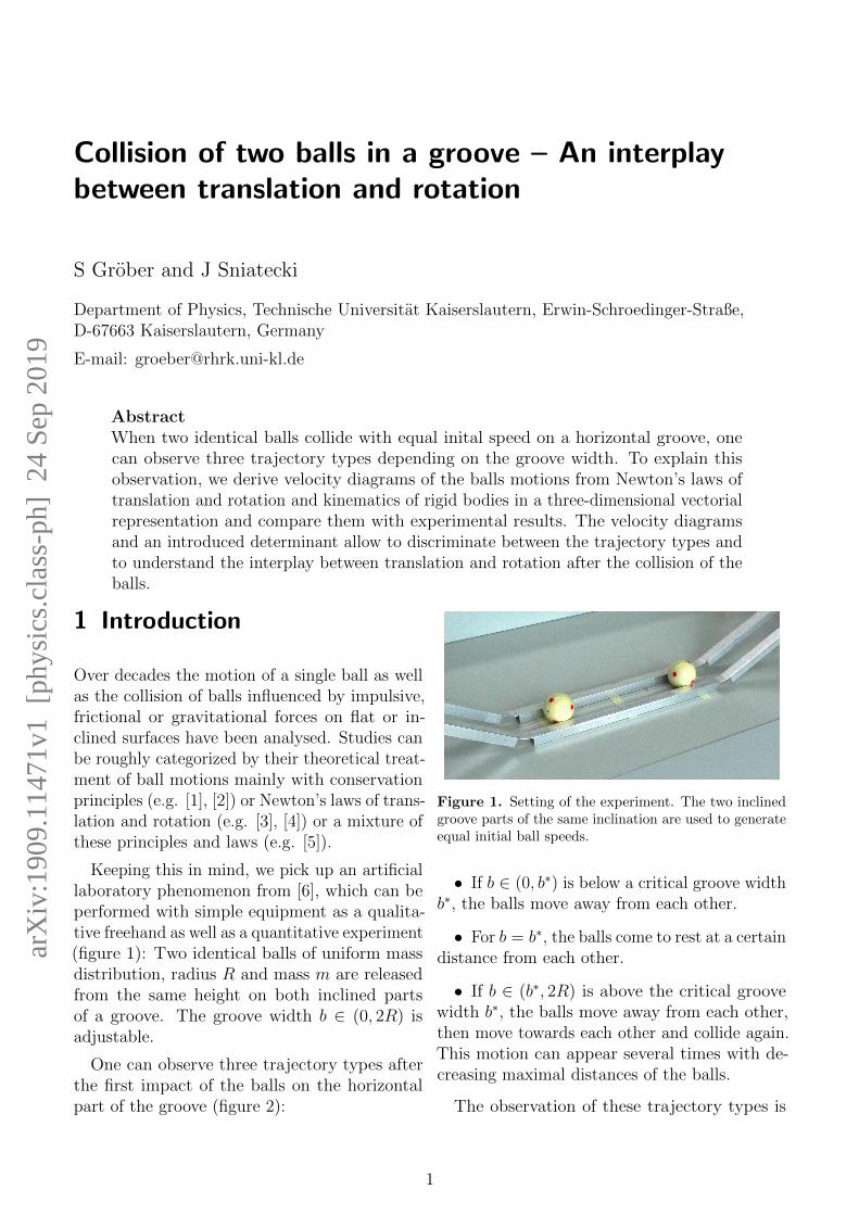
Keeping this in mind, we pick up an artificiallaboratory phenomenon from [6], which can beperformed with simple equipment as a qualita-tive freehand as well as a quantitative experiment(figure 1): Two identical balls of uniform massdistribution, radius R and mass m are releasedfrom the same height on both inclined partsof a groove. The groove width b ∈ (0, 2R) isadjustable.

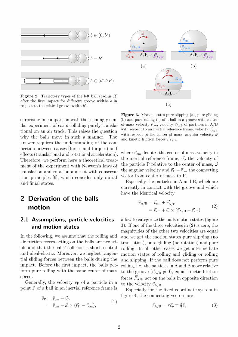
One can observe three trajectory types afterthe first impact of the balls on the horizontalpart of the groove (figure 2):

Figure 1. Setting of the experiment. The two inclinedgroove parts of the same inclination are used to generateequal initial ball speeds.

• If b ∈ (0, b∗) is below a critical groove widthb∗, the balls move away from each other.

• For b = b∗, the balls come to rest at a certaindistance from each other.

• If b ∈ (b∗, 2R) is above the critical groovewidth b∗, the balls move away from each other,then move towards each other and collide again.This motion can appear several times with de-creasing maximal distances of the balls.

The observation of these trajectory types is

1

arX

iv:1

909.

1147

1v1

[ph

ysic

s.cl

ass-

ph]

24

Sep

2019

b ∈ (0, b∗)

b = b∗

b ∈ (b∗, 2R)

Figure 2. Trajectory types of the left ball (radius R)after the first impact for different groove widths b inrespect to the critical groove width b∗.

surprising in comparison with the seemingly sim-ilar experiment of carts colliding purely transla-tional on an air track. This raises the questionwhy the balls move in such a manner. Theanswer requires the understanding of the con-nection between causes (forces and torques) andeffects (translational and rotational acceleration).Therefore, we perform here a theoretical treat-ment of the experiment with Newton’s laws oftranslation and rotation and not with conserva-tion principles [6], which consider only initialand finial states.

2 Derivation of the ballsmotion

2.1 Assumptions, particle velocitiesand motion states

In the following, we assume that the rolling andair friction forces acting on the balls are negligi-ble and that the balls’ collision is short, centraland ideal-elastic. Moreover, we neglect tangen-tial sliding forces between the balls during theimpact. Before the first impact, the balls per-form pure rolling with the same center-of-massspeed.

Generally, the velocity ~vP of a particle in apoint P of a ball in an inertial reference frame is

~vP = ~vcm + ~v′P= ~vcm + ~ω × (~rP − ~rcm),

(1)

~vA/B

~v′A/B~FA/B

A/B

~ω

(a)

~v′A/B

~vcm

A/B

~ω

(c)

~vA/B

~vcm

~FA/BA/B

(b)

Figure 3. Motion states pure slipping (a), pure gliding(b) and pure rolling (c) of a ball in a groove with center-of-mass velocity ~vcm, velocity ~vA/B of particles in A/Bwith respect to an inertial reference frame, velocity ~v′A/B

with respect to the center of mass, angular velocity ~ωand kinetic friction forces ~FA/B.

where ~vcm denotes the center-of-mass velocity inthe inertial reference frame, ~v′P the velocity ofthe particle P relative to the center of mass, ~ωthe angular velocity and ~rP−~rcm the connectingvector from center of mass to P.

Especially the particles in A and B, which arecurrently in contact with the groove and whichhave the identical velocity

~vA/B = ~vcm + ~v′A/B

= ~vcm + ~ω × (~rA/B − ~rcm)(2)

allow to categorize the balls motion states (figure3): If one of the three velocities in (2) is zero, themagnitudes of the other two velocities are equaland we get the motion states pure slipping (notranslation), pure gliding (no rotation) and purerolling. In all other cases we get intermediatemotion states of rolling and gliding or rollingand slipping. If the ball does not perform purerolling, i.e. the particles in A and B move relativeto the groove (~vA/B 6= ~0), equal kinetic friction

forces ~FA/B act on the balls in opposite directionto the velocity ~vA/B.

Especially for the fixed coordinate system infigure 4, the connecting vectors are

~rA/B = r~ey ∓ b2~ez (3)

2

r

R

b

x

y

z

contact points

circle of effectiveradius r

left ball

groove

cm

A

B

Figure 4. Fixed coordinate system and groove width b,radius R and effective radius r.

(minus for A and plus for B). Inserting (3) in(2) yields

~vA/B = vcm,x + (ωz~ez)× (r~ey ∓ b2~ez)

= (vcm,x − ωzr)~ex,(4)

In (4), the tangential velocity vt = ωzr of theparticles A and B on the circle of effective ra-dius r can be positive or negative, dependingon the sign of ωz and the direction of rotation,respectively.

In the following, due to symmetry, we consideronly the motion of the left ball. The originof the coordinate system is at the position ofthe center of mass of the left ball at the timet0 = 0, when the balls collide (figure 4). Beforethe first impact (t < t0) the ball performs purerolling with center-of-mass velocity vcm,x > 0and angular velocity ωz > 0, i.e. ~vA/B = 0 andfrom (4) follows the rolling condition

vcm,x = vt. (5)

Due to the assumptions, right after the impact,the center-of-mass velocity changed only in di-rection whereas the angular velocity and thetangential velocity vt keeps unchanged, i.e.

−vcm,x(t0) = vt(t0). (6)

The rolling condition is no longer fulfilled andkinetic friction forces act on the ball.

2.2 Center-of-mass and angularacceleration

To determine the center-of-mass acceleration ~acmand the angular acceleration ~α of the ball afterthe first impact, we apply Newton’s laws of trans-lation and rotation

~Fnet = m~acm (7)

and ~τnet = I~α. (8)

~Fnet denotes the net force on the ball, ~τnet thenet torque with respect to the center-of-massand I = 5

2mR2 the moment of inertia of the

ball with respect to an axis passing through thecenter of mass.

For both laws, we need to identify all forcesexerted on the ball. The groove exerts normalforces ~NA and ~NB on the ball in the contactpoints A and B, respectively. Because the ballmoves only in or against the x-direction, the y-and z-component of the net force is zero. There-fore, the normal forces and the weight force inthe y-z-plane compensate each other, i.e.

~NA + ~NB = −mg~ey. (9)

Due to symmetry, the y-components of thenormal forces are

NA/B,y = −1

2mg. (10)

According to figure 5 we get

|NA/B,y|| ~NA/B|

=r

R= k, (11)

with the ratio

k =r

R=

√1−

(b

2R

)2

, (12)

derived from figure 4. From (10) and (11) weget

| ~NA/B| =1

2kmg. (13)

The normal forces produce kinetic friction forces~FA and ~FB in the contact points A and B, respec-tively. These forces point in x-direction, becausethey are opposed to the velocity

vA/B,x(t0) = vcm,x(t0)− rωz(t0)= 2vcm,x(t0) < 0

(14)

3

(a)

z

y

x

~τA

~τB~NA

~NB

~τnet

~G~FA

~FB

cm

(b)

z

y

x

~τA

~τ B

~NA~NB

~τnet

~G~FA~FB

cm

Figure 5. Torques τA, τB and τnet due to the kineticfriction forces ~FA and ~FB, normal forces ~NA and ~NB andweight force ~G for a small (a) and greater groove widthb (b). In (b) the magnitude of the kinetic friction forcesis greater.

in x-direction. Application of the kinetic frictionlaw yields

~FA/B = µk| ~NA/B|~ex =1

2kµkmg~ex, (15)

where µk is the coefficient of kinetic friction.Overall, the net force on the ball is

~Fnet = ~FA + ~FB + ~NA + ~NB + ~G︸ ︷︷ ︸=~0

=1

kµkmg~ex.

(16)

According to (7) the center-of-mass’s accelera-tion

~acm =1

kµkg~ex. (17)

is constant, independent from the balls mass anddependent from the groove width.

For each force, we calculate the torque withrespect to the center of mass. The lines of actionof the normal forces ~NA/B and the weight force

~G pass through the center of mass, thus theirtorques are zero. The kinetic friction force ~FA

and ~FB causes the torque ~τA and ~τB, respectively.The torques are

~τA/B = (~rA/B − ~rcm)× ~FA/B. (18)

Inserting (3) and (15) in (18) yields

~τA/B = (r~ey ∓ b2~ez)× ( 1

2kµkmg~ex)

= − 12kµkmgr~ez ∓ b

4kµkmg~ey.

(19)

Hence, the y-component of the net torque ~τnet =~τA + ~τB is zero and we get

~τnet = −1

kµkmgr~ez = (r~ey)× (2~FA/B)

= −Rµkmg~ez.(20)

The net torque τnet is independent of the groovewidth b, because for increasing b the normalforces, the kinetic friction forces and thus theirtorques increase, but also the angle between thetorques (figure 5). According to (8) and (20) theangular acceleration

~α = −5µkg

2R~ez. (21)

is constant and independent from the balls massand the groove width.

2.3 Interplay between translationand rotation

Integrating (17) and (21) over the time intervall[t0, t] yields with (6) the linear functions

vcm,x(t) = vcm,x(t0) +µkg

kt, (22)

vt(t) = ωz(t)r = −vcm,x(t0)−5kµkg

2t. (23)

The signs in (22) and (23) indicate, that thegraphs of vcm,x(t) and vt(t) have for all k anintersection point at time t′0 (figure 6), when theball fulfills the rolling condition after the firstimpact, i.e.

vcm,x(t′0) = vt(t

′0). (24)

4

From (22)-(24) we obtain for t′0, vcm,x(t′0) and

the position x(t′0) =∫ t′00vcm,x(t) dt:

t′0 = − 4k

2 + 5k2vcm,x(t0)

µkg> 0 (25)

vcm,x(t′0) = −2− 5k2

2 + 5k2vcm,x(t0) = vt(t

′0) (26)

xcm(t′0) = − 20k3

2 + 5k2v2cm,x(t0)

µkg< 0. (27)

t

t0 tr0 t′0

vcm,x

vt (a)

t

t0 t′0 = tr0 = tt0

vcm,x

vt (b)

t

t0 tt0 t′0 t1 tt1 t′1

vcm,x

vt (c)

Figure 6. Theoretical graphs of the center-of-mass’velocity vcm,x(t) and the tangential velocity vt(t) forgroove widths b ∈ (0, b∗) (a), b = b∗ (b) and b ∈ (b∗, 2R)(c).

(26) allows to discriminate between the threetrajectory types:

• vcm,x(t′0) < 0 for b ∈ (0, b∗): The ball per-forms pure rolling for t > t′0 against the x-direction and the balls move apart from eachother. The center-of-mass velocity vcm,x remainsnegative after the impact, but the tangentialvelocity vt and the angular velocity ~ω changestheir direction according to (23) at the time

tr0 = − 2

5kµkgvcm,x(t0) ∈ [t0, t

′0]. (28)

At this time, the ball performs pure gliding (fig-ure 3(b)).

• vcm,x(t′0) = 0 for b = b∗, i.e. the balls cometo rest at time t′0. From (26) and (12) we get forthe critical groove width:

b∗

R=

√12

5. (29)

Neither the direction of translation nor the di-rection of rotation changes, because the rollingcondition is fulfilled at the moment the center-of-mass velocity is zero.

• vcm,x(t′0) > 0 for b ∈ (b∗, 2R): The ball isrolling in x-direction for t ≥ t′0 and the ballscollide again. The direction of rotation remainsthe same, whereas the direction of translationchanges according to (22) at the time

tt0 = − k

µkgvcm,x(t0) ∈ [t0, t

′0]. (30)

At this time the ball performs pure slipping(figure 3(a)).

Overall, the slopes of the vcm,x- and the vt-graph determine which of the three trajectorytypes occur. Therefore, the ratio

D =|at||acm,x|

=5

2k2 =

5

2

(1− b2

4R2

)(31)

is a determinant for the three trajectory types,where

at =dvtdt

= rαz (32)

denotes the tangential acceleration.

5

1

52

√52

√125

2

0 bR

|acm,x|µkg

|at|µkg

D = |at||acm,x|

Figure 7. Normalized center-of-mass accelera-tion |acm,x|/(µkg), normalized tangential acceleration|at|/(µkg) and ratio D against the ratio b/R.

For D ∈ (1, 52) and b ∈ (0, b∗), the tangential

acceleration at is greater than the center-of-massacceleration acm,x (figure 7). Translatory mo-tion decelerates faster than rotatory motion, andtherefore, the direction of translation changesbefore the direction of rotation could changeand the balls move apart. For D ∈ (0, 1) andb ∈ (b∗, 2R) the roles of translation and rotationare reversed, the balls move towards each otherand collide several times. For D = 1 and b = b∗

the center-of-mass and the tangential accelera-tion are equal in magnitude, i.e. the translatoryand rotatory motion synchronously deceleratetill the balls are at rest.

3 Comparison of theory andexperiment

For groove widths b of the three correspondingtrajectory types, the balls translatory and rota-tory motion was measured with video analysis[7] by tracking the center of mass coordinatesand the coordinates of a point on an circle ofeffective radius r with respect to a fixed coordi-nate system (frame rate of 100/s). Coordinatemeasurement errors were minimized by sufficienthigh ball radius and a selection of smallest possi-ble image section, which is adapted to the ball’smotion. We checked the equality of the initialball speeds and calculated the left ball’s center-of-mass velocity vcm,x and according to (4) the

0 0.2 0.4 0.6

−0.5

0

0.5

tr0 t′0

Vel

oci

ties

inm/s

vt(t)vcm,x(t)

−0.2 −0.1 0 0.1 0.2 0.3 0.4

−0.5

0

0.5

t′0

Vel

oci

ties

inm/s

0 0.2 0.4 0.6 0.8

−0.5

0

0.5

tt0 t′0

Time t in s

Vel

oci

ties

inm/s

Figure 8. Measured center-of-mass velocity vcm,x(t)and tangential velocity vt(t) for ball radius R = 2.75 cm,ball mass m = 0.167 kg and groove widths b = 3.5 cm (a),b = 4.4 cm (b) and b = 4.9 cm (c). Dashed lines indicatethe calculated times for pure gliding (a), for pure slipping(c) and the beginning of pure rolling (a)-(c).

6

b in cm |acm,x| inm/s2

µk,cm |~Fnet| inN

3.5 2.15 0.17 0.36

4.4 2.86 0.18 0.48

4.9 3.26 0.17 0.54

b in cm |at| inm/s2

µk,t |~τnet| inNm

3.5 2.92 0.15 0.008

4.4 2.61 0.17 0.009

4.9 2.00 0.16 0.008

Table 1. Experimentally determined quantities for theintermediate motion states after the first collision (fig-ure 1). The center-of-mass acceleration |acm,x| and thetangential acceleration |at| is determined from linear re-gression of vcm,x(t) and vt(t). Corresponding kineticfriction coefficient µk,cm and µk,t is calculated from the

slope in (22) and (23), respectively. The net force |~Fnet|and the net torque |~τnet| are calculated from (16) and(20) using µk = µk,cm.

tangential velocity vt (figure 6).

Equal magnitudes of vcm,x right before andafter the collision as well as the constant vcm,xin pure rolling time intervalls confirm the previ-ously made assumptions (see section 2.2). Theapproximately linear graphs of the intermediatemotion states confirm the use of the velocity-independent kinetic friction law (15).

The experimental results in table 1 indicatethat in accordance with the theory (figure 7,(16) and (20)) for increasing groove width b thecenter-of-mass acceleration acm,x and the net

force ~Fnet are increasing and the tangential ac-celeration at is decreasing, whereas the torque~τnet is approximately constant. The mean kineticfriction coefficient from table 1 is µk = 0.17.

4 Summary and educationalconclusions

In this article, we derived a cause-and-effectchain from particle kinematics and the applica-tion of Newton’s laws of translation and rotationfor rigid bodies to explain the three trajectorytypes when two identical balls collide with equal

speed in a groove of variable groove width (figure9). Overall, an increasing groove width causesan increasing center-of-mass and a decreasingtangential acceleration in magnitude, so thatwhen the rolling condition is fulfilled, the center-of-mass velocity either points away from thelocation of collision (the balls depart), is zero(the balls come to rest) or points towards thelocation of collision (the balls collide again).

Only when identical balls collide central andideal-elastic with equal initial speeds, the de-scription of the experiment can be restricted toone ball and the three trajectory types arise in-dependently of the initial speeds. Otherwise, themotions of the balls are asymmetric, depend onthe initial speeds and also on the inelasticity ofthe collision [1].

The theoretical level of the experiment pro-vides a challenging problem for introductory me-chanics courses. Explaining the occurence of thethree trajectory types in the experiment requiresto make appropriate assumptions, to apply andcombine several rigid body concepts and to per-form a quantitative analysis of the relations be-tween quantities. Therefore, students shouldhave sufficient previous knowledge about lawsand kinematics of rigid bodies from the lecture.We recommend to implement the experimentwith the here presented theoretical treatmentin homework problems or in the introductoryphysics laboratory [6], because there is sufficienttime for students to understand the experimen-tal results on their own. Additionally, teacherscan deal with the well known difficulties studentshave in understanding relevant rigid body con-cepts concerning the experiment, for example:

• Particle velocities of a rolling body withrespect to a fixed and a moved coordinate system[8].

• Independence of Newton’s law of translationfrom the working point of forces [9].

• A single force on a rigid body can causetranslation and rotation [9].

• Connection of kinetic friction forces andkinematics during the transition from rolling togliding [10].

7

b ↑(r ↓, k ↓)

~NA/B ↑ ~FA/B ↑

~Fnet ↑

~τnet = const.

(~α = const.)

|at| ↓

|acm,x| ↑

Rotation

Translation

b ∈ (0, b∗)|acm,x| < |at|

b = b∗|acm,x| = |at|

b ∈ (b∗, 2R)|acm,x| > |at|

Figure 9. Cause-and-effect chain to explain the occurence of the three trajectory types with groove width b,effective radius r, ratio k = r/R, normal forces ~NA/B, kinetic friction forces ~FA/B, net force ~Fnet, net torque ~τnet,angular acceleration ~α, center-of-mass acceleration acm,x and tangential acceleration at. ↑ and ↓ denotes increasingand decreasing in magnitude, respectively.

References

[1] Domenech A and Casasus E 1991 Frontalimpact of rolling spheres Phys. Educ. 26(3)186–189

[2] Redner S 2004 Billiard-theoretic approachto elementary one-dimensional elastic colli-sions Am. J. Phys. 72(12) 1492–1498

[3] Hierrezuello J 1993 Sliding and rolling: thephysics of a rolling ball Phys. Educ. 30(3)177–182

[4] Hopkins D C and Patterson J D 1977 Bowl-ing frames: paths of a bowling ball Am. J.Phys. 45(3) 263–266

[5] Wallace R E and Schroeder M C 1988 Anal-ysis of billiard ball collisions in two dimen-sions Am. J. Phys. 56(9) 815–819

[6] Hanisch C, Hofmann F and Ziese M 2018Linear momentum, angular momentum andenergy in the linear collision between twoballs Eur. J. Phys. 39(1) 015003

[7] Allain R 2016 Physics and video analysis(San Rafael: Morgan & Claypool Publish-ers)

[8] Rimoldini L G and Singh C 2005 Studentunderstanding of rotational and rolling mo-tion concepts Phys. Rev. Phys. Educ. Res.1(1) 010102

[9] Close H G, Gomez L S and Heron P R L2013 Student understanding of the appli-cation of newton’s second law to rotatingrigid bodies Eur. J. Phys. 81(6) 458–470

[10] Ambrosis A, Malgieri M, Mascheretti P andOnorato P 2015 Investigating the role ofsliding friction in rolling motion: a teachingsequence based on experiments and simula-tions Eur. J. Phys. 36(3) 035020

8