Munich Personal RePEc Archive

Collusion in Quality-Segmented Markets

Bos, Iwan and Marini, Marco A.

Department of Organisation, Strategy and Entrepreneurship,

Maastricht University, Department of Social and Economic Sciences,

University of Rome La Sapienza and CREI

1 October 2020

Online at https://mpra.ub.uni-muenchen.de/106338/

MPRA Paper No. 106338, posted 09 Mar 2021 20:51 UTC

Collusion in Quality-Segmented Markets∗

Iwan Bos† Marco A. Marini‡

October 2020

Abstract

This paper analyzes price collusion in a repeated game with two submarkets; a standard and apremium quality segment. Within this setting, we study four types of price-fixing agreement: (i)a segment-wide cartel in the premium submarket only, (ii) a segment-wide cartel in the standardsubmarket only, (iii) two segment-wide cartels, and (iv) an industry-wide cartel. We present acomplete characterization of the collusive pricing equilibrium and examine the corresponding effecton market shares and welfare. Partial cartels operating in a sufficiently large segment lose marketshare and the industry-wide cartel prefers to maintain market shares at pre-collusive levels. Theimpact on consumer and social welfare critically depends on the cost of producing quality. Moreover,given that there is a cartel, more collusion can be beneficial for society as a whole.

Keywords: Partial Cartels, Price Collusion, Market Segmentation, Vertical Differentiation.

JEL Classification: D4, L1 .

∗We appreciate the comments of and discussions with David Collie, Luis Corchón, Jean Gabszewicz, Andrey Minaev,Riccardo Saulle, Attila Tasnádi, Jacques-François Thisse and participants at the Oligo Workshop in Nottingham. Allopinions and errors are ours alone.

†Iwan Bos, Department of Organisation, Strategy and Entrepreneurship, Maastricht University. E-mail:i.bos@maastrichtuniversity.nl.

‡University of Rome La Sapienza and CREI. Mailing Address: Department of Social and Economic Sciences, PiazzaleAldo Moro, 5, 00185, Rome, Italy. Email: marco.marini@uniroma1.it.

1

1 Introduction

Virtually all markets can be segmented by product variety or customer group. In principle there are

many segmentation dimensions, but perhaps the most common one is (perceived) quality. Quality

submarkets emerge due to factors on both the demand and the supply side. On the demand side,

differences exist in the ability and willingness to pay for product quality. On the supply side, there are

typically larger costs associated with the production of higher quality goods and services. The presence

of such quality segments has a nontrivial effect on firms’ strategies and on pricing in particular.

The purpose of this paper is to examine price collusion in quality-segmented markets. We do so by

studying a price-setting supergame with two quality submarkets; a standard and a premium segment.

It is assumed that products within each segment are perfect substitutes and that they are differentiated

across segments. In the spirit of Mussa and Rosen (1978), Gabszewicz and Thisse (1979) and Shaked and

Sutton (1982), consumers have heterogeneous valuations for quality and buy from the firm with the best

value proposition. Within this setting, we consider four types of price-fixing agreement: (i) a segment-

wide cartel in the premium submarket only, (ii) a segment-wide cartel in the standard submarket only,

(iii) two segment-wide cartels, one in each submarket, and (iv) an industry-wide cartel.

It is worth noting that these scenarios have been observed in (antitrust) practice. For example,

a recent German coffee roaster cartel consisted exclusively of premium brands and faced competition

from lower quality private labels (e.g., store brands of Aldi and Lidl).1 During the interwar period, an

incomplete Swiss dyestuff export cartel competed with inferior quality rivals from other countries.2 By

contrast, a French yogurt cartel fixed prices of supermarket own-brand yogurt, but premium producers

like Danone did not participate in the collusive agreement.3 As yet another example, a German sausage

cartel spanned a large part of the market and included both private label and premium brands.4

With this in mind, we employ our model to address questions such as: what does optimal segment-

wide collusion look like? How does price-fixing affect the market share of the quality-segments? What

are the welfare implications of the different types of price conspiracies? Is a cartel in a premium segment

more or less detrimental to consumers and society at large than a cartel in a standard quality segment?

We begin our analysis by providing a complete characterization of the collusive price equilibrium for

all four scenarios. Each partial coalition is shown to be capable of sustaining the joint profit maximum,

whereas the industry-wide cartel charges monopoly prices only when its members are sufficiently patient.

1See Hasnas and Wey (2015).2See Schmitt and Weder (1998) for a detailed description of this cartel.3See Bonnet and Bouamra-Mechemache (2019).4See Hasnas and Wey (2015). The grocery examples are appealing because there typically is a clear difference between

the (perceived) quality of the private label products and the premium brands. However, our analysis is not limited tosuch situations and effectively applies to any industry with distinct quality segments. Moreover, it also applies to casesof tacit collusion. For instance, even though there was no explicit cartel case, there is evidence of price collusion betweentwo premium ice cream brands, Ben & Jerry’s and Häagen-Dazs, for the year 2013. See Sullivan (2017).

2

Cartel prices are increasing with the inclusiveness of the coalition. That is, prices are higher when

collusion spans the whole market and the industry-wide cartel sets (weakly) higher prices compared to

when there are two segment-wide partial cartels. The latter is driven by the fact that the all-inclusive

cartel internalizes the pricing externality across segments.

These collusive equilibria have an impact on the market share distribution. If there is a single

segment-wide cartel, then there is a net movement of customers to the non-collusive segment. With

two partial cartels, the change in segment size effectively depends on the competitive market share. If a

segment is sufficiently small absent collusion, then cartel prices are set such that its sales share increases

(and vice versa). The all-inclusive cartel prefers to maintain market shares at pre-collusive levels, which

requires prices to rise more in the premium segment. It is noteworthy that such a market division rule

has been frequently observed in antitrust practice.5 Also, we have assumed such an allocation scheme

in Bos and Marini (2019), whereas here it emerges endogenously.

As to welfare, we delineate two distinct effects: a market size effect and a market share effect. The

market size effect is the change in welfare that comes from buyers leaving the market. Part of the

consumers in the standard segment derive little value from quality and they may no longer buy the

product when its price increases. This market size effect is therefore absent when there is a partial

cartel in the premium segment only since in that case the price of the standard quality product remains

unaltered. In the other three scenarios, the price of the standard product rises so that the market

size effect is strictly negative. The market share effect describes the movement of customers from one

segment to the other. Since the value created is larger in the premium segment, this effect is positive

when more consumers buy the high quality product. By contrast, it is negative when customers switch

from the premium to the standard quality segment. These distinct effects, and in particular the fact

that they might work in opposite directions, make the welfare impact of the different types of price

conspiracy far from trivial.

We find that customer damages increase with the inclusiveness of the cartel, which is in line with

expectations. Yet, whether a single partial cartel in the premium or in the standard submarket is more

harmful effectively depends on the relation between quality and costs. Specifically, a single cartel in the

standard segment is more detrimental to buyers when unit costs rise sufficiently with quality. In that

case, sellers in the standard segment have a relatively strong market position and this enables them

to sustain a relatively high cartel price. This induces many buyers to leave the market, i.e., there is

a strong negative market size effect which significantly harms consumer welfare. In a similar vein, the

impact on societal welfare also depends on the degree to which costs increase with quality. Among

others, we find that the (positive) market share effect may outweigh the (negative) market size effect.

This has the implication that a single segment-wide cartel may be more detrimental to society than two

segment-wide partial cartels. Therefore, given that there is collusion in one segment, a social planner

5See, for example, Harrington (2006).

3

might well prefer collusion over competition in the adjacent segment.

Our research is naturally related to studies on collusion in markets with vertically differentiated

products.6 Häckner (1994) and Symeonides (1999), for instance, both analyze how the incentive to

chisel on a collusive agreement depends on quality and reach opposite conclusions. In Bos and Marini

(2019), we add to this by arguing that profit margins are a critical driver of deviating incentives. Ecchia

and Lambertini (1997) explore the impact of a minimum quality standard and establish that such a

standard can make it harder for firms to collude. Recently, Bos, Marini and Saulle (2020) show that

generally there is a strong incentive to coordinate prices when the products involved are differentiated

vertically. A key difference with all this and related work is that firms are supposed to take a unique

position along the quality spectrum, whereas here we consider quality segments in which two or more

sellers offer the same quality.7

Another related strand of research considers heterogeneity in cartel size. For instance, Donsimoni

(1985) examines a collusive price leadership model with differences in production costs. She shows the

existence of a stable, less than all-inclusive cartel comprising the most efficient firms. Consistent with

this result, Bos and Harrington (2010) find that the incentive to collude is positively related to firm

size and that sufficiently small sellers may prefer not to take part in the anti-competitive coalition.

More recently, de Roos and Smirnov (2020) study pricing strategies of a partial cartel assuming that

consumers are imperfectly attentive. Among other things, they characterize the optimal collusive price

path and show it may involve intertemporal price dispersion. Finally, Bos, Marini and Saulle (2020)

establish that many different cartel sizes may emerge when products are vertically differentiated. None

of these works considers partial collusion in quality-segmented markets, however.

This paper proceeds as follows. The next section introduces the model. In Section 3, we use

this setting to study partial and full price collusion. Section 4 builds on this by presenting a welfare

analysis. Section 5 concludes with a summary and suggestions for further work. All proofs are relegated

to Appendix A.

2 Model

Consider an industry with two quality segments; a low (standard) and a high (premium) quality segment.

Let the set of low and high quality sellers be respectively given by L = {1, . . . , l} and H = {1, . . . , h},with l, h ≥ 2. Each firm supplies a single quality variant of the product so that l+h is the total numberof firms.8 Within each segment, sellers are identical and their quality is indicated by vi, where i = l, h

6For a detailed overview of this literature, see Marini (2018).7Hasnas and Wey (2015) study partial and full collusion in a three-firm spatial setting. They effectively consider a

high quality segment in the sense that two horizontally differentiated premium producers are assumed to offer the samequality and face a lower quality private label firm. In our model, each quality variant is supplied by two or more sellersand firms within a particular segment solely compete on price.

8We elaborate on the possibility of multi-product firms in Appendix B.

4

and vh > vl > 0. Corresponding marginal costs of production are constant per unit of output and

given by ch ≥ cl ≥ 0. It is therefore weakly more expensive to manufacture the high quality product.Interaction takes place for an infinite number of discrete periods and in each period t ∈ N producerssimultaneously pick prices to maximize their profits. The discount factor is δ ∈ (0, 1) and all prices setup until t− 1 are assumed common knowledge.The demand side comprises consumers who are uniformly distributed over [0, 1] with a mass nor-

malized to unity. The parameter θ describes the degree to which buyers value quality and a higher θ

corresponds to a higher gross utility when consuming variant vi. Consumers either purchase one unit

of the product or choose an outside option for which the valuation is normalized to zero. Someone

‘located’ at θ therefore obtains the following utility:

U(θ) =

{θvi − pi when buying quality i

0 when not buying,(1)

where pi ∈ R+ is the price set by a firm offering quality vi, i = l, h. Observe that this specification

implicitly assumes firms within one segment to set the same price; a property that we verify below.

To further economize on notation, we write pl and ph to indicate the prices set in the standard and

premium segment, respectively. Finally, it is worth noting that some consumers prefer not to buy the

product when prices are strictly positive in which case the market is not covered.

Let us now describe the demand for each firm. To begin, a consumer ‘located’ at θ0 is indifferent

between buying from a firm i ∈ L and the outside option when:

θ0vl − pl = 0⇒ θ0 =plvl.

In a similar vein, a consumer at θ1 is indifferent between buying from a firm i ∈ L and a firm i ∈ Hwhen:

θ1vl − pl = θ1vh − ph ⇒ θ1 =ph − plvh − vl

.

Under the assumption that consumers spread evenly across equally-priced firms, firm demand is then

given by:

Dl (pl, ph) =θ1 − θ0l

=vlph − vhpll (vh − vl) vl

,

and

Dh (pl, ph) =1− θ1h

=vh − vl − ph + plh (vh − vl)

,

with concomitant profit functions:

πl (pl, ph) = (pl − cl) ·[vlph − vhpll (vh − vl) vl

], (2)

5

and

πh (pl, ph) = (ph − ch) ·[vh − vl − ph + plh (vh − vl)

]. (3)

In the ensuing analysis, we concentrate on situations in which each firm is active (i.e., has strictly

positive sales). The following two assumptions provide sufficient conditions for an interior solution:

Assumption 1. 1 >ch − clvh − vl

>clvl.

Assumption 2. Each firm chooses ‘to be productive’ over ‘not to be productive’ when both yield the

same profit.

The first assumption ensures that production costs are not ‘too high’ in relation to the quality of the

products and the valuation thereof. The second assumption states that firms have a weak preference

for positive sales. An implication of these assumptions is that there is a unique static Nash equilibrium

in which each seller sets price at marginal costs. Thus, none of them makes an economic profit absent

collusion. Below, we indicate this noncollusive outcome with a superscript ‘*’.

3 Collusion

We now proceed by considering the possibility of firms colluding on supra-competitive prices. In the

following, four scenarios are studied: (1) segment-wide collusion in the low-quality submarket only, (2)

segment-wide collusion in the high-quality submarket only, (3) segment-wide collusion in both submar-

kets separately and simultaneously, and (4) industry-wide collusion. For all these cases, we characterize

the optimal collusive contract under the assumption that conspirators’ aim is to maximize joint profits

and a deviation from the agreement by any of them results in infinite reversion to the static Nash

equilibrium.

3.1 Partial collusion

To begin, suppose that collusion is not industry-wide so that conspirators receive competition from

firms not taking part in the agreement. Since our focus is on segment-wide collusion, a partial cartel

faces one of the following two constrained maximization problems:

maxpl

1

1− δ · (pl − cl) ·[vlph − vhpl(vh − vl) vl

], subject to (4)

δ ≥ δ∗l ≡ 1−1

l· (pl − cl) (vlph − vhpl)(pdl − cl

) (vlph − vhpdl

) ,

or

6

maxph

1

1− δ · (ph − ch) ·[vh − vl − (ph − pl)

vh − vl

], subject to

δ ≥ δ∗h ≡ 1−1

h· (ph − ch) (vh − vl − (ph − pl))(pdh − ch

) (vh − vl − pdh + pl

) ,

where the superscript ‘d’ denotes the optimal deviating price.9

Let us now discuss the deviating strategy in more detail. Notice first that, given the profitability

of the cartel, it never pays to cheat by lifting the price since this would leave the deviant firm with no

demand. Next, shaving price slightly below the collusive segment price would yield one hundred percent

of the sales in this particular submarket. However, whether this is the optimal deviating strategy

depends on the best-reply toward the adjacent segment. If that price is lower than the collusive price,

then a deviating firm finds it in its interest to follow this best-response. Consequently, pdi = min {pci , p̃i},i = l, h, where pci indicates the collusive price and p̃i is the best-reply price toward the adjacent quality

segment.10

The next proposition specifies optimal prices in the event of a standard segment partial cartel, a

premium segment partial cartel and a partial cartel in both segments simultaneously. The superscript

indicates the type of price-fixing conspiracy under consideration.

Proposition 1. If there is a price cartel in the standard segment only, then

pll =vl2vh

ch +1

2cl,

plh = ch.

If there is a price cartel in the premium segment only, then

phl = cl,

phh =vh − vl + cl + ch

2.

If there is a price cartel in the standard segment and in the premium segment, then

plhl =(vh − vl) vl + 2vhcl + vlch

4vh − vl,

plhh =2 (vh − vl) vh + vhcl + 2vhch

4vh − vl.

9The critical discount factor δ∗lis obtained by rearranging the following incentive compatibility constraint:

1

1− δ · (pl − cl) ·vlph − vhpll (vh − vl) vl

≥(pdl− cl

)· vlph − vhp

d

l

(vh − vl) vl.

The critical discount factor δ∗hcan be derived in a similar fashion. Notice that this specification gives one hundred percent

market segment share to a deviant firm; something that will be verified in the ensuing analysis.10Note that when p̃i > p

c

i, pd

ishould, strictly speaking, be the maximum price below pc

i. Yet, this is problematic since

action sets are continuous in our model. We therefore follow the convention by simply writing pdi= pc

iin this case, which

effectively means that the deviant seller prices arbitrarily close to pciand obtains all demand in the respective market

segment(s). See, amongst many others, Tirole (1988), Bos and Harrington (2010), and de Roos and Smirnov (2020).

7

As a first observation, note that there is a single optimum in all three scenarios. Specifically, each partial

cartel is capable of sustaining the joint profit maximum. The reason is that the profit-maximizing price

is a best-response to the price set in the adjacent quality segment. This means that the optimal deviating

strategy is to undercut the cartel price by the smallest possible amount, i.e., pdi = pci , i = l, h. In turn,

this has the implication that the incentive compatibility constraints reduce to:

δ ≥ δ∗l = 1−1

l, and

δ ≥ δ∗h = 1−1

h.

Thus, the unconstrained solution is feasible whenever some collusion is sustainable. Given a high enough

discount factor, the latter requires the number of firms in the segment to be sufficiently small.

Next, it can be easily verified that cartel prices are higher when firms in the adjacent segment are also

colluding, which is due to the strategic complementarity of the choice variables. In terms of comparative

statics, cartel prices are rising with unit production costs in both segments. Moreover, in case of a single

segment-wide partial cartel, prices are increasing with the own quality level and decreasing with the

quality offered in the noncollusive segment.

Yet, the effect of changes in quality is more subtle when there are two partial cartels. Similar to the

case of a single segment-wide cartel, the collusive price of the premium product is increasing in vh and

decreasing in vl. This is less straightforward in the standard segment, however. To see this, note that:

dplhldvl

=∂plhl∂vl

+∂plhl∂plhh

· dplhh

dvl=(4vh − vl) · (vh − 2vl + ch) + (vh − vl) vl + 2vhcl + vlch

(4vh − vl)2,

dplhldvh

=∂plhl∂vh

+∂plhl∂plhh

· dplhh

dvh=(4vh − vl) · (vl + 2cl)− 4 (vh − vl) vl − 8vhcl − 4vlch

(4vh − vl)2.

Hence, dplhl /dvl < 0 and dplhl /dvh > 0 when unit costs are (approximately) zero and the quality differ-

ence, vh − vl, is small enough. In both cases, the sign of the direct effect is as expected (∂plhl /∂vl > 0and ∂plhl /∂vh < 0). However, the indirect (or strategic) effect may work in the opposite direction

(∂plhl /∂plhh ·dplhh /dvl < 0 and ∂plhl /∂plhh ·dplhh /dvh > 0) and dominates the direct effect when the situation

is sufficiently symmetric.

We conclude this subsection by considering the shifts in market shares resulting from partial collusion.

Let sl and sh indicate the sales share of the standard and premium segment, respectively. The next result

shows how the size of the respective segments changes under the different (partial) collusive scenarios.

Corollary 1. If there is a price cartel in the standard segment only, then

sll < s∗l ,

slh > s∗h.

8

If there is a price cartel in the premium segment only, then

sll > s∗l ,

slh < s∗h.

If there is a price cartel in the standard segment and in the premium segment, then

slhl < s∗l and slhh > s

∗

h when (vl − cl) s∗l > (vh − ch) s∗h,slhl > s∗l and s

lhh < s

∗

h when (vl − cl) s∗l < (vh − ch) s∗h.

The change in market shares in case of a single segment-wide cartel is in line with the existing literature.

Theoretical work on incomplete cartels robustly predict a decrease in demand for the colluding firms’

products and an increase in demand for non-cartel suppliers.11 The Corollary reveals that the standard

and premium segment partial cartels not only lose buyers in absolute terms, but also in relative terms,

i.e., their share of total sales decreases.

In case of two partial cartels, the change in market share depends on the segment sizes absent

collusion as well as the value created. If, say, the premium segment is relatively small and it is relatively

costly to provide additional quality (i.e., both s∗h and vh− ch are ‘small’ and s∗l and vl − cl are ‘large’),then the price increase in the premium segment is smaller than in the standard segment. The strong

market position of the sellers in the standard segment allows them to raise their price significantly. By

contrast, the weak market position of the premium suppliers limits the scope for a price increase. Since

in this case it holds that plhl − cl > plhh − ch, some buyers move from the standard to the premium

segment so that high quality suppliers gain back some market share.

3.2 Full collusion

We now direct our attention to the possibility of an all-inclusive cartel. In comparison to the partial

cartel cases that we have analyzed above, such a collusive contract is more sophisticated in the sense

that the anti-competitive combination has to simultaneously select a price for both segments. Formally,

the industry-wide cartel faces the following constrained optimization problem:

maxpl,ph

1

1− δ ·[(ph − ch) ·

vh − vl − ph + plvh − vl

+ (pl − cl) ·vlph − vhpl(vh − vl) vl

], subject to

11See, e.g., de Roos (2001), Bos and Harrington (2010), Inderst, Maier-Rigaud and Schwalbe (2014) as well as thereferences therein.

9

δ ≥ δ∗l ≡ 1−1

l· (pl − cl) (vlph − vhpl)(pdl − cl

) (vlph − vhpdl

) , and

δ ≥ δ∗h ≡ 1−1

h· (ph − ch) (vh − vl − (ph − pl))(pdh − ch

) (vh − vl − pdh + pl

) .

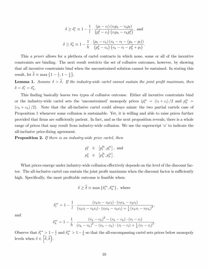
This a priori allows for a plethora of cartel contracts in which none, some or all of the incentive

constraints are binding. The next result restricts the set of collusive outcomes, however, by showing

that all incentive constraints bind when the unconstrained solution cannot be sustained. In stating this

result, let δ̃ ≡ max{1− 1

l, 1− 1

h

}.

Lemma 1. Assume δ > δ̃. If the industry-wide cartel cannot sustain the joint profit maximum, then

δ = δ∗l = δ∗

h.

This finding basically leaves two types of collusive outcome. Either all incentive constraints bind

or the industry-wide cartel sets the ‘unconstrained’ monopoly prices (pml = (vl + cl) /2 and pmh =

(vh + ch) /2). Note that the all-inclusive cartel could always mimic the two partial cartels case of

Proposition 1 whenever some collusion is sustainable. Yet, it is willing and able to raise prices further

provided that firms are sufficiently patient. In fact, and as the next proposition reveals, there is a whole

range of prices that may result from industry-wide collusion. We use the superscript ‘a’ to indicate the

all-inclusive price-fixing agreement.

Proposition 2. If there is an industry-wide price cartel, then

pal ∈[plhl , p

ml

], and

pah ∈[plhh , p

mh

].

What prices emerge under industry-wide collusion effectively depends on the level of the discount fac-

tor. The all-inclusive cartel can sustain the joint profit maximum when the discount factor is sufficiently

high. Specifically, the most profitable outcome is feasible when:

δ ≥ δ̂ ≡ max {δ∗∗l , δ∗∗h } , where

δ∗∗l = 1−1

l· (vhvl − vhcl) · (vlch − vhcl)(vhvl − vhcl) · (vlch − vhcl) + 1

4(vhvl − vlch)2

,

and

δ∗∗h = 1−1

h· (vh − ch)2 − (vh − ch) · (vl − cl)(vh − ch)2 − (vh − ch) · (vl − cl) + 1

4(vl − cl)2

.

Observe that δ∗∗l > 1− 1land δ∗∗h > 1− 1

hso that the all-encompassing cartel sets prices below monopoly

levels when δ ∈[δ̃, δ̂).

10

The previous result presents the profit-maximizing prices. Assuming the joint profit maximum, the

following proposition specifies the profit-maximizing production level for each cartel participant.

Proposition 3. Assume an industry-wide cartel and suppose that δ ≥ δ̂. Each participant produces

precisely half its Nash demand:

Dal =

1

2D∗

l ,

Dah =

1

2D∗

h.

The next result follows almost immediately.

Corollary 2. Assume an industry-wide cartel and suppose that δ ≥ δ̂. All market shares are maintainedat pre-collusive levels.

This is a remarkable result for at least two reasons. First, we have studied full collusion under

quality differentiation elsewhere assuming that the industry-wide cartel maintains market shares at

pre-collusive levels.12 This finding shows that the cartel may find it in its interest to select this market

division scheme when collusion spans several quality-segments simultaneously. Second, the literature on

collusion in vertically differentiated markets has repeatedly shown that it may well be optimal to price

lower-quality products out of the market.13 Such a strategy is suboptimal within our setting due to the

substantial difference in production costs (as specified by Assumption 1). Indeed, and in line with the

existing literature, it would be optimal to exclusively sell the premium product when the cost difference

is sufficiently small.

4 Welfare

The previous section provides a complete characterization of collusive pricing for the different types of

cartel agreement. Let us now turn to the welfare consequences. We start with analyzing the impact on

consumer welfare and then proceed by examining the effect on societal surplus.

4.1 Consumer Surplus

How are consumers affected by the different types of price-fixing agreement? To answer this question,

we begin by presenting the benchmark of no collusion. Recall that the static Nash equilibrium has all

firms price at marginal cost. In this case, therefore, a buyer who is indifferent between staying at home

and purchasing the low quality item is ‘located’ at θ∗0 = cl/vl. A consumer who is indifferent between the

12See Bos and Marini (2019).13See, for example, Bos, Marini and Saulle (2020). An overview of this literature is provided by Marini (2018). In fact,

as total market demand is inversely related to the price of the standard product, this market share allocation implies thatthe price increase is larger in the premium segment.

11

standard and the premium product is at θ∗1 = (ch − cl) / (vh − vl). Combining gives the (net) consumersurplus (henceforth CS):

CS∗ =

∫ 1

θ∗0

U(θ)dθ =

∫ (ch−cl)(vh−vl)

cl/vl

(θ · vl) dθ − cl · l ·Dl +

∫ 1

(ch−cl)(vh−vl)

(θ · vh) dθ − ch · h ·Dh

=(vh − 2ch) · (vh − vl) + (ch − cl)2 +

(vh−vlvl

)· c2l

2 (vh − vl),

which is decreasing in price (cl and ch) and increasing in quality (vl and vh).

Now consider the four collusive scenarios studied above. For any of these cases, consumer surplus is

generally given by:

CS =

∫ 1

θ0

U(θ)dθ =

∫ ph−plvh−vl

plvl

(θ · vl) dθ − pl · l ·Dl +

∫ 1

ph−plvh−vl

(θ · vh) dθ − ph · h ·Dh.

By Proposition 1 and Proposition 2, we know that prices differ for the different cartel regimes. The

next result shows how the various price-fixing agreements rank in terms of their impact on consumer

welfare. To facilitate comparison between the different scenarios, we assume without loss of generality

that cl = 0 and c = ch − cl.Proposition 4. There is a threshold k ∈ (0, 1) such that:(i) If c/ (vh − vl) < k, then

CS∗ > CSl > CSh > CSlh ≥ CSa, and

(ii) If c/ (vh − vl) > k, thenCS∗ > CSh > CSl > CSlh ≥ CSa.

Not surprisingly, collusion is bad for buyers. The industry-wide cartel is the most harmful and, also

in line with expectations, the scenario of two segment-wide partial cartels is second worst. The ranking

of single segment-wide cartels is sensitive to differences in costs and quality, however. Specifically, if a

substantial quality improvement can be obtained for little additional cost, then a partial cartel in the

premium segment is more detrimental to consumers. By contrast, a single partial cartel in the standard

segment is more harmful when unit costs rise sufficiently with quality.

To see the intuition behind this latter result consider two extreme scenarios. If c/ (vh − vl)→ 0, then

low quality firms are unable to effectively compete with their high quality rivals, either in competition or

under collusion. In this case, premium suppliers offer a superior value proposition even when pl = cl = 0.

A cost difference is thus necessary for a standard segment-wide cartel to be viable and raise price to

12

supra-competitive levels. More generally, the impact of such a cartel on consumer welfare remains

limited when low quality suppliers have a relatively weak market position as reflected by a low c or a

high vh − vl.By contrast, if c/ (vh − vl) → 1, then a partial cartel in the standard segment increases its price

substantially above costs. This not only induces some customers to switch from the standard to the

premium segment, but it also makes some buyers leave the market. Note that the latter effect is not

present when there is a single partial cartel in the premium segment. As part (ii) of Proposition 4

reveals, this reduction in market size may be sufficiently strong to make consumers worse off with a

cartel in the standard segment.

4.2 Social Welfare

What about the welfare of society as a whole? How do the various types of cartel agreement affect

societal surplus? To address this issue, we shall evaluate the following general social welfare function:

SW (pl, ph) =

∫ ph−plvh−vl

plvl

(θ · vl) dθ − cl ·(ph − plvh − vl

− plvl

)+

∫ 1

ph−plvh−vl

(θ · vh) dθ − ch ·(1− ph − pl

vh − vl

).

As established in Proposition 1 and Proposition 2, prices will differ for the different scenarios, and

consequently so will societal surplus.

We start the comparison with the next proposition, which reveals the preference of a social planner.

Proposition 5. A Social Planner would charge prices equal to marginal costs:

pl = cl and ph = ch.

Since prices are set at marginal costs in both segments absent collusion and each cartel raises price

above costs, the implication of this result is that social welfare is highest when there is no cartel. Not

surprisingly, therefore, a social planner prefers a competitive world.

Let us now turn to the other extreme; an industry-wide cartel. As before, we assume without loss

of generality that cl = 0 and c = ch − cl to facilitate comparison between the different scenarios.Proposition 6. Social welfare under all forms of partial collusion is (weakly) higher than with an

industry-wide cartel.

This result confirms the intuition of an all-inclusive price-fixing cartel being most detrimental to

society as a whole. As the proof in the Appendix reveals, this holds both when the incentive constraints

are binding and when the industry-wide cartel is capable of sustaining the monopoly solution. In fact,

societal surplus monotonically declines gradually when both segment prices continuously increase along

the intervals as specified in Proposition 2.

13

As the next proposition shows, the same does not hold for partial cartels.

Proposition 7. Define ρ ≡√2/2 + 3/4.

(i) If vh/vl = ρ, then there exists a unique threshold k ∈ (0, 1) such that:

if c/ (vh − vl) < k, then SW l > SW lh > SW h,

if c/ (vh − vl) > k, then SW h > SW lh > SW l.

(ii) If vh/vl > ρ, then there exist three thresholds k1, k2, k3 ∈ (0, 1), with k3 > k2 > k1, such that:

if c/ (vh − vl) ∈ (0, k1), then SWl > SW lh > SW h,

if c/ (vh − vl) ∈ (k1, k2), then SWl > SW h > SW lh,

if c/ (vh − vl) ∈ (k2, k3), then SWh > SW l > SW lh,

if c/ (vh − vl) ∈ (k3, 1), then SWh > SW lh > SW l.

(iii) If vh/vl < ρ, then there exist three thresholds k1, k2, k3 ∈ (0, 1), with k1 > k2 > k3, such that:

if c/ (vh − vl) ∈ (0, k3), then SWl > SW lh > SW h,

if c/ (vh − vl) ∈ (k3, k2), then SWlh > SW l > SW h,

if c/ (vh − vl) ∈ (k2, k1), then SWlh > SW h > SW l,

if c/ (vh − vl) ∈ (k1, 1), then SWh > SW lh > SW l.

This result reveals that the impact of partial cartels on societal surplus is everything but trivial. In

fact, each partial collusion scenario can be most or least detrimental to society and two cartels can be

better than one.

To explain the intuition underlying this finding it is useful to distinguish between two distinct effects:

a market size effect and a market share effect. The first captures the impact on social welfare that comes

from a reduction in market size due to a raise in the standard segment price. It can be easily verified

that the magnitude is increasing in the price of the low quality product. This implies that it is lowest for

a single premium segment-wide cartel (in fact, it is zero because in that case pl = cl like in competition)

and highest in case of two partial cartels. Note further that this effect is weakly negative so that absent

any other effect we would have SW h > SW l > SW lh.

Yet, there is a second effect that is driven by a shift in market shares. This market share effect cap-

tures the extent to which buyers are induced to switch to the segment generating most value. Following

Assumption 1, the value created is higher in the premium segment. Hence, collusion may positively affect

societal surplus by incentivizing consumers of standard products to switch to the premium segment.

14

With these two concepts in mind, let us now compare social welfare in case of a single partial

cartel: SW h and SW l. To start, note that the market size effect is zero in case of a single premium

cartel. Moreover, the price rise in the premium segment induces some buyers to move to the standard

segment so that the market share effect is negative. A single standard segment-wide cartel is worse in

terms of the market size effect since it is strictly negative. At the same time, however, it incentivizes

buyers to move to the premium segment so that the market share effect is positive. Proposition 7 shows

that this positive market share effect sufficiently mitigates the negative market size effect when the cost

difference is sufficiently low and the quality gap is sufficiently high. In other words, a single cartel in

the premium segment is more detrimental to society than a single cartel in the standard segment when

the value created in the premium segment, vh − ch, is significantly higher than the value created in thestandard segment, vl − cl.With regards to the two partial cartels scenario, note that compared to a single premium cartel the

negative market size effect is stronger since the standard segment price is higher (plhl > phl ). The market

share effect is less negative, however. The above result reveals that the market size effect dominates the

market share effect when the marginal production costs of quality are high. In that case, the difference

in value created between segments is limited and SW h > SW lh. By contrast, the market share effect

may dominate the market size effect when marginal production costs of quality are low in which case it

holds that SW lh > SW h.

Finally, comparing the two partial cartels scenario with a single segment-wide cartel in the standard

segment, the former has a stronger market size effect (since plhl > pll). As to the market share effect,

this effectively depends on the price difference between the standard and the premium quality segment.

Specifically, the difference is smaller in the two partial cartel case when the marginal production costs

of quality is sufficiently high:

plhh − plhl < plh − pll ⇔2vh

(2vh − vl)<

c

(vh − vl).

Proposition 7 shows that the market share effect may be sufficiently strong to make a single standard

segment cartel more detrimental than two segment-wide cartels.

In sum, what partial cartels are most harmful for society critically depends on the differences in cost

and quality. A partial cartel in the premium (standard) segment is more detrimental to society when

the difference in value created between both segments is sufficiently high (low), all else unchanged.

5 Concluding Remarks

In many industries, firms can be grouped into more homogeneous classes based on quality. We have

addressed the question of what collusion may look like in such quality-segmented markets through

studying an infinitely repeated price-setting game with two submarkets; a standard and a premium

15

quality segment. We used this framework to analyze four types of price-fixing agreement: a segment-

wide cartel in the premium submarket only, a segment-wide cartel in the standard submarket only,

two segment-wide cartels, one in each submarket, and an industry-wide cartel. For all these cases, we

provided a complete characterization of the collusive equilibrium and examined the impact on market

shares and welfare.

Let us summarize some of our main findings. Partial cartels are capable of sustaining the joint

profit maximum, whereas the all-inclusive cartel can sustain the unconstrained optimum only when its

members are sufficiently patient. Incomplete cartels loose market share when the segment in which they

operate is sufficiently large and the industry-wide cartel prefers to set its prices such to maintain market

shares at pre-collusive levels. In terms of welfare, we show that a partial cartel in the premium segment

is more detrimental to consumers than a partial cartel in the standard segment when the marginal costs

of quality are sufficiently small. The impact on societal welfare also critically depends on the relation

between quality and costs. Among other things, we find that a single segment-wide partial cartel may

be more harmful for society than two segment-wide partial cartels.

There are three natural avenues for future research. First, it may be interesting to also allow for

within-segment heterogeneity, i.e., include some degree of horizontal differentiation. Second, one might

explore the potential impact of additional quality segments. Both extensions will likely prove to be

computationally challenging, however. Finally, we have studied price collusion given qualities. Though

it seems natural to assume the available qualities to be exogenous in the short run, we can imagine

situations in which the quality offered is (partly) endogenous. It is worth exploring how our main

findings would be affected when allowing firms to reposition themselves along the quality spectrum. We

leave this issue for future research.

16

6 Appendix A: Proofs

Proof of Proposition 1. To start, consider a single segment-wide partial cartel in the standard

segment. Such a cartel faces the following constrained maximization problem:

maxpl

1

1− δ · (pl − cl) ·vlph − vhpl(vh − vl) vl

subject to

δ ≥ δ∗l = 1−1

l· (pl − cl) (vlph − vhpl)(pdl − cl

) (vlph − vhpdl

) .

Since there is more than one firm in the adjacent premium segment, it follows from Assumption 1

and Assumption 2 that ph = ch. This means that the joint profit-maximizing price is a best-reply to

ch, which implies pdl is (approximately) equal to this collusive solution. The incentive compatibility

constraint therefore reduces to:

δ ≥ δ∗l = 1−1

l.

Consequently, the joint profit-maximizing price can be sustained whenever some collusion is sustainable.

Taking the first-order condition and rearranging gives:

pll =vl2vh

ch +1

2cl.

Next, consider a single segment-wide partial cartel in the premium segment. Such a cartel faces the

following constrained maximization problem:

maxph

1

1− δ · (ph − ch) ·vh − vl − ph + pl

vh − vlsubject to

δ ≥ δ∗h = 1−1

h· (ph − ch) (vh − vl − ph + pl)(pdh − ch

) (vh − vl − pdh + pl

) .

Since there is more than one firm in the standard segment, it follows from Assumption 1 and Assumption

2 that pl = cl. Similar to the previous case, the joint profit-maximizing price is a best-reply to cl, which

implies pdh is (approximately) equal to this collusive solution. The incentive compatibility constraint

therefore reduces to:

δ ≥ 1− 1

h.

The joint profit-maximizing price can thus be sustained whenever some collusion is sustainable. Taking

the first-order condition and rearranging gives:

phh =vh − vl + cl + ch

2.

Finally, consider the possibility of a partial cartel in each segment. Also in this case, the joint

profit-maximizing price is a best-response to the price set by firms in the adjacent segment. Thus, pdi ,

17

i = l, h, is again (approximately) equal to this collusive solution and the incentive constraints reduce

to:

δ ≥ 1− 1l, and δ ≥ 1− 1

h.

Hence, the joint profit-maximizing prices can be sustained whenever some segment-wide collusion is

feasible. The collusive optimum is therefore given by the respective first-order conditions. Rearranging

gives:

plhl =(vh − vl) vl + 2vhcl + vlch

4vh − vl,

plhh =2 (vh − vl) vh + vhcl + 2vhch

4vh − vl.

Proof of Corrolary 1. To begin, note that the market shares of the two segments absent collusion

are given by:

s∗l =chvl − clvh

(vh − vl) (vl − cl),

s∗h =vl (vh − vl − ch + cl)(vh − vl) (vl − cl)

.

Using the collusive prices as specified in Proposition 1, when there is a partial cartel in the standard

segment only its sales share is:

sll =chvl − pllvh

(vh − vl)(vl − pll

) = vh (chvl − clvh)(vh − vl) (2vhvl − chvl − clvh)

,

which is smaller than the Nash equilibrium share when:

sll − s∗l =vh (chvl − clvh)

(vh − vl) (vl (vh − ch) + vh (vl − cl))− chvl − clvh(vh − vl) (vl − cl)

< 0.

Rearranging gives:

−vl (vh − ch) < 0,

which holds.

Using the collusive prices as specified in Proposition 1, when there is a partial cartel in the premium

segment only its sales share is:

shh =vl(vh − vl − phh + cl

)

(vh − vl) (vl − cl)=vl (vh − vl − ch + cl)2 (vh − vl) (vl − cl)

,

which is smaller than the Nash equilibrium share when:

18

shh − s∗h =vl (vh − vl − ch + cl)2 (vh − vl) (vl − cl)

− vl (vh − vl − ch + cl)(vh − vl) (vl − cl)

< 0,

which holds.

Finally, consider the case in which there is a partial cartel in both segments. We show that slhh > s∗

h

when (vl − cl) s∗l > (vh − ch) s∗h. By the prices as specified in Proposition 1, slhh is given by:

slhh =vl(vh − vl − plhh + plhl

)

(vh − vl)(vl − plhl

) =vl [2vh (vh − vl)− 2chvh + chvl + clvh](vh − vl) [vl (vh − ch) + 2vh (vl − cl)]

.

Comparing with the Nash equilibrium share:

slhh > s∗hvl [2vh (vh − vl)− 2chvh + chvl + clvh](vh − vl) [vl (vh − ch) + 2vh (vl − cl)]

>vl (vh − vl − ch + cl)(vh − vl) (vl − cl)

.

Rearranging and using the above specifications for s∗l and s∗

h gives:

(vl − cl) · s∗l > (vh − ch) · s∗h.

Hence, we conclude that if (vl − cl) s∗l > (vh − ch) s∗h, then slhl < s∗l and slhh > s∗h (and vice versa).Proof of Lemma 1. To begin, note that the all-inclusive cartel could mimic the situation with

two segment-wide partial cartels as specified in Proposition 1. Yet, since δ > δ̃ ≡ max{1− 1

l, 1− 1

h

},

the industry-wide cartel can improve upon this outcome. Next, recall that the joint profit-maximizing

prices in the two partial cartels case are in fact best-responses to the adjacent segment. This has the

implication that when the cartel increases prices further it holds that pdi = p̃i, i = l, h. That is, a deviant

firm finds it optimal to not just cut its price slightly below the collusive segment price, but to lower it

further to the best-reply level.

Given this deviating strategy, let us now proceed by writing down the Lagrangian of the constrained

maximization problem:

L (pl, ph) =1

1− δ ·[(ph − ch) ·

vh − vl − ph + plvh − vl

+ (pl − cl) ·vlph − vhpl(vh − vl) vl

]

+λ1 ·[(ph − ch) ·

vh − vl − ph + plvh − vl

− (1− δ) · h · (vh − vl + pl − ch)2

4 (vh − vl)

]

+λ2 ·[(pl − cl) ·

vlph − vhpl(vh − vl) vl

− (1− δ) · l · (vlph − vhcl)2

4vh (vh − vl) vl

].

The corresponding Karush-Kuhn-Tucker (KKT) conditions are:

19

∂L

∂ph=

1

1− δ · [vh − vl − 2ph + 2pl + ch − cl] + λ1 · [vh − vl − 2ph + pl + ch]

+λ2 ·[pl − cl − (1− δ) · l ·

(vlph − vhcl)2vh

]= 0

∂L

∂pl=

1

1− δ ·[2vlph − 2vhpl + vhcl − vlch

vl

]

+λ1 ·[ph − ch − (1− δ) · h ·

(vh − vl + pl − ch)2

]+ λ2 ·

[vlph − 2vhpl + vhcl

vl

]= 0

λ1, λ2 ≥ 0

λ1 ·[(ph − ch) · (vh − vl − ph + pl)− (1− δ) · h ·

(vh − vl + pl − ch)24

]= 0

λ2 ·[(pl − cl) · (vlph − vhpl)− (1− δ) · l ·

(vlph − vhcl)24vh

]= 0

To show that all incentive constraints must be binding when the joint profit maximum cannot be

sustained, we consider two cases: (i) the incentive constraints of all high-quality firms are binding,

whereas the incentive constraints of the low-quality firms are not and (ii) the incentive constraints of all

low-quality firms are binding, whereas the incentive constraints of the high-quality firms are not. For

both cases, we derive a contradiction.

Case (i): λ1 > 0 and λ2 = 0. In this case, the KKT conditions reduce to:

∂L

∂ph=

1

1− δ · [vh − vl − 2ph + 2pl + ch − cl] + λ1 · [vh − vl − 2ph + pl + ch] = 0

∂L

∂pl=

1

1− δ ·[2vlph − 2vhpl + vhcl − vlch

vl

]

+λ1 ·[ph − ch − (1− δ) · h ·

(vh − vl + pl − ch)2

]= 0

λ1 > 0, λ2 = 0

λ1 ·[(ph − ch) · (vh − vl − ph + pl)− (1− δ) · h ·

(vh − vl + pl − ch)24

]= 0.

As the price of the basic good is unconstrained, we know that:

2vlph − 2vhpl + vhcl − vlchvl

= 0.

20

Hence, by the second KKT condition it must hold that:

ph − ch − (1− δ) · h ·(vh − vl + pl − ch)

2= 0,

whereas by the last KKT condition, we know:

(ph − ch) · (vh − vl − ph + pl)− (1− δ) · h ·(vh − vl + pl − ch)2

4= 0

⇔ ph − ch = (1− δ) · h ·(vh − vl + pl − ch)24 (vh − vl − ph + pl)

.

Combining gives:

(1− δ) · h · (vh − vl + pl − ch)2

4 (vh − vl − ph + pl)− (1− δ) · h · (vh − vl + pl − ch)

2= 0,

or

vh − vl − 2ph + pl + ch = 0.

Combining with the first KKT condition, this implies:

vh − vl − 2ph + pl + ch + pl − cl = 0,

which cannot hold as pl > cl under collusion; a contradiction.

Case (ii): λ1 = 0 and λ2 > 0. In this case, the KKT conditions reduce to:

∂L

∂ph=

1

1− δ · [vh − vl − 2ph + 2pl + ch − cl] + λ2 ·[pl − cl − (1− δ) · l ·

(vlph − vhcl)2vh

]= 0

∂L

∂pl=

1

1− δ ·[2vlph − 2vhpl + vhcl − vlch

vl

]+ λ2 ·

[vlph − 2vhpl + vhcl

vl

]= 0

λ1 = 0, λ2 > 0

λ2 ·[(pl − cl) · (vlph − vhpl)− (1− δ) · l ·

(vlph − vhcl)24vh

]= 0.

As the price of the premium product is unconstrained, we know that:

vh − vl − 2ph + 2pl + ch − cl = 0.

Hence, by the first KKT condition it must hold that:

pl − cl − (1− δ) · l ·(vlph − vhcl)

2vh= 0,

21

whereas by the last KKT condition, we know that:

(pl − cl) · (vlph − vhpl)− (1− δ) · l ·(vlph − vhcl)2

4vh= 0⇔

pl − cl = (1− δ) · l ·(vlph − vhcl)24vh (vlph − vhpl)

.

Combining gives:

(1− δ) · l · (vlph − vhcl)24vh (vlph − vhpl)

− (1− δ) · l · (vlph − vhcl)2vh

= 0,

or

vlph − 2vhpl + vhcl = 0.

Combining with the second KKT condition, this implies:

vlph − 2vhpl + vhcl + vlph − vlch = 0,

which cannot hold as ph > ch under collusion, a contradiction. We thus conclude that when a profit-

maximizing industry-wide cartel sets prices below the joint profit maximum all incentive constraints

must be binding.

Proof of Proposition 2. Industry-wide collusion is sustainable when:

δ ≥ δ∗l = 1−1

l· (pl − cl) (vlph − vhpl)(pdl − cl

) (vlph − vhpdl

) , and

δ ≥ δ∗h = 1−1

h· (ph − ch) (vh − vl − ph + pl)(pdh − ch

) (vh − vl − pdh + pl

) .

To begin, the all-inclusive cartel can mimic the two partial cartels scenario as described in Proposition

1. In that case, pal = pdl and p

ah = p

dh so that the incentive constraints reduce to:

δ ≥ 1− 1l, and δ ≥ 1− 1

h.

Thus, the industry-wide cartel can sustain the following prices whenever some collusion is sustainable:

pil = plhl =(vh − vl) vl + 2vhcl + vlch

4vh − vl, and

pih = plhh =2 (vh − vl) vh + vhcl + 2vhch

4vh − vl.

This would be the outcome when δ = δ̃.

If δ > δ̃, then the industry-wide cartel is able and willing to raise prices further. In that case,

deviating prices are a best-response to the adjacent quality segment and strictly below the collusive

22

level. Using pdl = (vlpah + vhcl) /2vh and p

dh = (vh − vl + pal + ch) /2, the critical discount factors can be

written as:

δ∗l = 1− 1l· (pl − cl) (vlph − vhpl)(pdl − cl

) (vlph − vhpdl

) = 1− 1l·[2(pdl − cl

)(pl − cl)− (pl − cl)2(pdl − cl

)2

], and

δ∗h = 1− 1

h· (ph − ch) (vh − vl − ph + pl)(pdh − ch

) (vh − vl − pdh + pl

) = 1− 1

h·[2(pdh − ch

)(ph − ch)− (ph − ch)2(pdh − ch

)2

].

Note that, in both cases, the last term between brackets is strictly below 1 so that the incentive

constraints are tighter than in the scenario with two partial cartels. By Lemma 1, when collusion is

constrained, the industry-wide cartel sets its prices such that δ = δ∗l = δ∗

h.

Finally, if δ → 1, then none of the incentive constraints bind in which case collusive prices are given

by the first-order conditions. Rearranging gives:

pal = pml =

vl + cl2

, and pah = pmh =

vh + ch2

.

Proof of Proposition 3. Using the full collusive unconstrained prices as specified in Proposition 2,

the profit-maximizing production levels are given by:

Dal =

vlch − vhcl2lvl (vh − vl)

,

Dah =

(vh − vl)− ch + cl2h (vh − vl)

,

which is precisely half the Nash demand:

D∗

l =vlch − vhcll (vh − vl) vl

,

D∗

h =(vh − vl)− ch + cl

h (vh − vl).

Proof of Corollary 2. Absent collusion, total market demand is given by

D∗ =vl − clvl

.

Under full collusion at the joint profit maximum, it is:

Da =vl − cl2vl

.

Combining with the results from the previous proposition, it can be easily verified that

Dai

Da=D∗

i

D∗,∀i ∈ L,H.

23

Proof of Proposition 4. To begin, note that consumer surplus can be written as:

CS =

∫ ph−plvh−vl

plvl

(θ · vl) dθ − pl ·vlph − vhpl(vh − vl) vl

+

∫ 1

ph−plvh−vl

(θ · vh) dθ − ph ·vh − vl − ph + pl

vh − vl

=p2h +

vhvlp2l − 2ph (pl + vh − vl) + vh (vh − vl)

2 (vh − vl),

which is monotonically decreasing in both prices. Hence, all types of cartel are bad for buyers in the

sense that at least one consumer pays more for the same quality and no consumer pays less. It follows

that consumer surplus is highest absent collusion. Moreover, since consumer welfare is strictly decreasing

in segment prices, it holds that CSl, CSh > CSlh (by Proposition 1) and CSlh ≥ CSa (by Proposition2). We conclude that CS∗ > CSl, CSh > CSlh ≥ CSa.Finally, let us compare CSl and CSh. Combining the consumer surplus formula with the prices

given in Proposition 1, one obtains:

CSl =4 (vh − vl) (vh − c)2 + vlc2

8vh (vh − vl), and

CSh =(vh − vl) (vh + 3vl − 2c) + c2

8 (vh − vl).

Taking the difference yields:

CSl − CSh = 3vh (vh − vl − 2c) + 3c28vh

,

which for c→ 0 reduces to3vh (vh − vl)

8vh> 0.

Next, CSl − CSh is convex in c and negative at the upper bound, c = vh − vl (Assumption 1):

−3vh (vh − vl) + 3 (vh − vl)28vh

< 0.

Also note that:

CSl − CSh = 3vh (vh − vl − 2c) + 3c28vh

= 0⇒ c2 − 2cvh + vh (vh − vl) = 0,

which has c̃ = vh −√vhvl as the smaller root. Combining these findings then leads to the following

conclusion. For a given quality gap vh − vl: (i) if c ∈ [0, c̃), then CSl > CSh, and (ii) if c ∈ (c̃, vh − vl),then CSh > CSl.

24

Proof of Proposition 5. First, note that social welfare is generally given by:

SW (pl, ph) =

∫ ph−plvh−vl

plvl

(θ · vl) dθ − cl ·(ph − plvh − vl

− plvl

)+

∫ 1

ph−plvh−vl

(θ · vh) dθ − ch ·(1− ph − pl

vh − vl

),

yielding

SW (pl, ph) =vlvh (vh − vl) + 2cl (plvh − phvl)− vlph (ph − 2pl)− p2l vh − 2vlch (pl − ph + vh − vl)

2 (vh − vl) vl.

Next, note that the Hessian is negative definite:

d2SW (pl, ph)

dp2h= − 1

(vh − vl)< 0,

d2SW (pl, ph)

dp2l= − vh

vl (vh − vl)< 0,

d2SW (pl, ph)

dpldph= 0.

Hence,

det

[− 1(vh−vl)

0

0 − vh(vl−vh)vl

]> 0.

The social optimum is thus given by the first-order conditions.

dSW (pl, ph)

dph= 0⇒ ph = ch + pl − cl,

dSW (pl, ph)

dph= 0⇒ pl = cl +

phvl − chvlvh

.

Combining gives:

pl = cl and ph = ch.

Proof of Proposition 6. Let us first consider the case where δ ≥ δ̂ ≡ max {δ∗∗l , δ∗∗h } so that theindustry-wide cartel will set the unconstrained monopoly prices as specified in Proposition 2. Combining

the collusive prices as given in Proposition 1 and Proposition 2 with the general social welfare function

gives:

SW l =8cvhvl + 4v

2h (vh − vl)− 4cvh (2vh − c)− c2vl

8vh (vh − vl),

SW h =3c (c+ 2vl)− 6cvh − v2l + vh (3vh − 2vl)

8 (vh − vl),

SW lh =2vh (6v

3h + v

3l )− 2vhc (12v2h + 5v2l ) + 2c2v2l − vlv2h (13vh + vl) + vlvhc (34vh − 9c) + 12c2v2h

2 (vh − vl) (4vh − vl)2,

SW a =3 (vh − vl) (vh − 2c) + 3c2

8 (vh − vl).

25

Comparing the societal surplus under a single segment-wide cartel regime with the social welfare

with a industry-wide cartel yields:

SW l − SW a =(vh − c)28vh

> 0,

SW h − SW a =1

8vl > 0.

Next, let us compare social welfare under the two partial cartels scenario with social welfare under

unconstrained full collusion:

SW lh − SW a = vl ·(vh − vl) (vh (20vh − 11vl)− 2c (4vh − 3vl))− (12vh − 5vl) c2

8 (vh − vl) (4vh − vl)2.

Notice that SW lh − SW a > 0 for c→ 0 and that the difference SW lh − SW a decreases monotonically

in c. Substituting the upper bound c = vh − vl (Assumption 1) in SW lh − SW a gives:

v2l (20vh − 11vl)8 (4vh − vl)2

> 0.

We conclude that social welfare under partial collusion is strictly higher than under an industry-wide

cartel capable of sustaining the joint profit maximum.

Finally, let us consider the case where δ ∈[δ̃, δ̂)so that the industry-wide cartel sets prices

below the monopoly level. We show that social welfare declines when the incentive constraints are

binding and the prices set by the firms continuously increase along the interval ranging from the two

partial cartels to the industry-wide cartel prices as specified in Proposition 2.

Now suppose that both incentive constraints are binding (Lemma 1) and consider a marginal increase

in the discount factor. The binding incentive constraints are given by:

(ph − ch) · (vh − vl − ph + pl)− (1− δ) · h ·(vh − vl + pl − c)2

4= 0

pl · (vlph − vhpl)− (1− δ) · l ·(vlph)

2

4vh= 0

Since a marginal increase in the discount factor relaxes both incentive constraints this yields an

increase in collusive prices. Specifically, we can distinguish a direct effect and an indirect effect. The

latter comes from the fact that a price increase in one segment enables a price increase in the adjacent

segment. Using the binding incentive constraints and solving for ph and pl yields:

ph(pl) =1

2(c+ vh − vl + pl) +

1

2

√(h (δ − 1) + 1) (vh − vl − c+ pl)2 (5)

pl(ph) =1

4v2h

[2phvhvl + 2

√p2hv

2hv2l (l (δ − 1) + 1)

]. (6)

26

These expressions show that the two prices ph and pl are positively related. Starting with an increase

in ph, the impact on social welfare is

dSW

dph= −dpl(ph)

dphvl −

1− dpldph

vh − vl· (vh − vl − c) = −

dpl(ph)

dphvl −

(1− dpl(ph)

dph

)·D∗

h · h.

The first term captures the market size effect. Since an increase in ph has a positive indirect effect

on pl this effect is negative. The second term captures the market share effect. If ph increases, then

some customers move to the standard segment. This effect is, however, countered by the indirect

positive effect on pl. Nevertheless, a sufficient condition for the market share effect to be negative is

that dpl(ph)dph

< 1, which holds because 0 < (l (δ − 1) + 1) < 1 and:

dpldph

=vl2vh

((l (δ − 1) + 1) phvhvl√(l (δ − 1) + 1) p2hv2hv2l

+ 1

)< 1.

Let us now turn to the increase of pl. The impact on social welfare is given by:

dSW

dpl=1

vl· (−vl) +

dphdpl− 1

vh − vl· (vh − vl − c) = −1−

(1− dph

dpl

)·D∗

h · h < 0.

As before, the first term captures the market size effect and the second term captures the market

share effect. Since dphdpl

≥ 0 and D∗

h · h < 1, the combined effect is negative. Taken together, societal

surplus therefore gradually decreases when prices increase marginally along the interval as specified in

Proposition 2. We conclude that SW lh ≥ SW a.

Proof of Proposition 7. Social welfare under the different partial cartel scenarios is provided in the

proof of Proposition 6. Comparing them yields the following thresholds in reference to k = c/(vh − vl):

SW h T SW lh ⇔ c/ (vh − vl) T k1 ≡ (4vh + vl) / (12vh − 5vl) ∈ (0, 1) ,SW h T SW l ⇔ c/ (vh − vl) T k2 ≡ (vh −

√vhvl) / (vh − vl) ∈ (0, 1) ,

SW lh T SW l ⇔ c/ (vh − vl) T k3 ≡ [2 (4vh − 3vl) vh] /(8v2h − 2vhvl + v2l

)∈ (0, 1) .

It can be readily verified that there is a quality-ratio:

vh/vl = ρ ≡√2/2 + 3/4,

for which all thresholds are equal, i.e., k1 = k2 = k3. Moreover, if vh/vl > ρ, then k1 > k2 > k3 and if

vh/vl < ρ, then k3 > k2 > k1. The welfare ranking under the different partial cartel regimes as specified

in the proposition then follows accordingly.

27

7 Appendix B: Multi-product Firms

The analyses in this paper have been performed under the assumption that each producer offers a single

quality. Alternatively, sellers may simultaneously supply multiple quality variants. In this appendix, we

briefly discuss how allowing for such multi-product firms might affect our main findings. To be clear, a

multi-product firm within our framework is a firm with two divisions; one in each segment. All other

assumptions are as above.

To begin, it can be easily verified that the presence of multi-product firms does not alter the impact

of the all-inclusive cartel. The reason is that in our setting the industry-wide cartel de facto operates

as a multi-plant monopolist, which implies that all pricing externalities are internalized. Therefore,

and irrespective of the number of multi-product members, prices are as given by Proposition 2. In

light of the main analysis above, these prices are also sustainable since the incentive constraint of a

multi-product firm is effectively a combination of incentive constraints of two independently operating

quality divisions.

Next, consider the case of two segment-wide partial cartels. How would the presence of multi-

product firms affect the collusive outcome as specified in Proposition 1? To address this question, let

the number of multi-product firms be given by k ≥ 0. The collusive best-replies of the standard and

premium segment-wide cartels are then respectively given by:

plhl =vl(1 + k

h

)plhh + vhcl − k

hvlch

2vh,

and

plhh =(vh − vl) +

(1 + k

h

)plhl + ch − k

lcl

2.

Note that when there are no multi-product firms (k = 0), the collusive outcome is the same as in

Proposition 1. By contrast, if all firms would sell both quality variants (k = l = h), then the joint

profit maximum coincides with that of an industry-wide cartel (Proposition 2). In general, the more

multi-product firms in this case, the larger the extent to which pricing externalities are internalized and

the higher are the profit-maximizing prices.

This solution is feasible whenever some collusion is sustainable. The reason is as follows. Since the

collusive segment price is weakly below the best-response to the collusive price in the other segment,

the optimal deviating strategy is to undercut the collusive price(s) by the smallest possible amount.

This implies that incentive compatibility is effectively only determined by the discount factor and the

number of firms involved. In fact, the incentive constraint of a multi-product firm is less tight than that

of a single-product seller in this case since deviating in one submarket induces a lower cartel price in

the adjacent segment.

Finally, let us discuss the possibility of a single segment-wide partial cartel with one or more multi-

product members. In this situation, the collusive best-reply functions are the same as above. The key

28

difference with the two segment-wide partial cartels case is, however, that the price in the noncollusive

segment equals marginal costs when the number of outsiders exceeds two. Therefore, independent of

the number of multi-product firms, prices remain as in Proposition 1.

Yet, this situation changes when there are only two firms active in the adjacent segment. To see

this, suppose there is a single partial cartel in the premium submarket. Suppose further that k = 1 and

l = 2. The multi-product firm could now contemplate the following strategy. Rather than keeping price

at costs in the standard segment it may increase this price. This implies that the multi-product firm

sacrifices all its market share in the low quality submarket, because the best-reply by the outsider is

to price below it. Such a strategy is nevertheless profitable since profits remain zero in the low quality

submarket and increase in the premium segment. The latter is due to the strategic complementarity of

the choice variable.

To see that this strategy is also feasible, consider the incentive constraint of the multi-product firm

when it would indeed set price above costs in the standard segment:

1

1− δ · (pch − ch) ·

vh − vl − pch + pl(vh − vl)h

≥(pdh − ch

)· vh − vl − p

dh + pl

(vh − vl)+(pdl − cl

)· vlp

ch − vhpl

(vh − vl) vl.

First note that in this case the multi-product firm faces a tighter incentive constraint than single-

product firms because its deviating profits are (weakly) higher, whereas collusive profits are the same.

Second, since price exceeds costs in the standard segment, the optimal deviating strategy for the multi-

product firm is to cut price in both submarkets simultaneously. Finally, the outsider charges a price

weakly below the best-response to the collusive premium price and that collusive price itself is weakly

below the best-response to the price in the low quality segment. Optimal deviating prices are therefore

(approximately) equal to the segment prices, i.e., pdh = pch and pdl = pl. This reduces the incentive

constraint of the multi-product firm to:

[1− (1− δ)h] · (pch − ch) (vh − vl − pch + pl)− (1− δ)h · (pl − cl)vlp

ch − vhplvl

≥ 0.

Provided that some collusion is sustainable, the collusive price pch is the same as in Proposition 1

when pl = cl. However, the above strategy is also feasible for a high enough discount factor. In fact, if

δ → 1, then the multi-product firm could set and sustain the best-responses: pl = (vlpch + vhcl) /2vh and

pch = (vh − vl + pl + ch) /2. Notice that these are precisely the prices that would result in case of twosegment-wide partial cartels. In a similar vein, multi-product firms may lead to higher collusive prices

when there is a single segment-wide cartel in the standard segment and there are two firms active in

the adjacent premium segment.

In sum, in most cases the presence of multi-product firms does not affect the collusive outcome, but

when it does, cartel prices are higher. This can occur when there are two partial cartels or when there

is a single partial cartel and there are two firms active in the adjacent segment.

29

References

[1] Bonnet, C. and Z. Bouamra-Mechemache (2019), Yogurt Cartel: Yogurt Cartel of Private Label

Providers in France: Impact on Prices and Welfare, TSE Working Papers 19-1012, Toulouse School

of Economics.

[2] Bos, Iwan and Joseph E. Harrington Jr. (2010), “Endogenous Cartel Formation with Heterogeneous

Firms,” RAND Journal of Economics, 41(1), 92-117.

[3] Bos, Iwan, Marco A. Marini and Riccardo Saulle (2020), “Cartel Formation with Quality Differen-

tiation,” Mathematical Social Sciences, 106, 33-50.

[4] Bos, Iwan and Marco A. Marini (2019), “Cartel Stability under Quality Differentiation,” Economics

Letters, 174, 70-73.

[5] De Roos, Nicolas and Vladimir Smirnov (2020), “Collusion, Price Dispersion, and Fringe Compe-

tition,” Working Paper, Sydney University.

[6] De Roos, Nicolas (2001), “Collusion with a Competitive Fringe: An Application to Vitamin C,”

Working Paper, Yale University.

[7] Donsimoni, Marie-Paule (1985), “Stable Heterogeneous Cartels,” International Journal of Indus-

trial Organization, 3(4), 451-467.

[8] Ecchia, Giulio and Luca Lambertini (1997), “Minimum Quality Standards and Collusion,” Journal

of Industrial Economics, 45(1), 101-113.

[9] Gabszewicz, Jean J. and Jacques-François Thisse (1979), “Price Competition, Quality and Income

Disparities,” Journal of Economic Theory, 20(3), 340-359.

[10] Häckner, Jonas (1994), “Collusive Pricing in Markets for Vertically Differentiated Products,” In-

ternational Journal of Industrial Organization, 12(2), 155-177.

[11] Harrington, Joseph E. Jr. (2006), “How do Cartels Operate?,” Foundations and Trends in Micro-

economics, 2(1), 1-105.

[12] Hasnas, Irina and Christian Wey (2015), “Full versus Partial Collusion among Brands and Private

Label Producers,” DICE Discussion Paper, 190.

[13] Inderst, Roman, Frank P. Maier-Rigaud, and Ulrich Schwalbe (2014), “Umbrella Effects,” Journal

of Competition Law & Economics, 10(3), 739-763.

30

[14] Marini, Marco A. (2018), “Collusive Agreements in Vertically Differentiated Markets,” in Handbook

of Game Theory and Industrial Organization, Volume 2: Applications, Luis C. Corchón and Marco

A. Marini (eds.), Edward Elgar, Chelthenam, UK, Northampton, MA, USA.

[15] Mussa, Michael and Sherwin Rosen (1978), “Monopoly and Product Quality,” Journal of Economic

Theory, 18(2), 301-317.

[16] Schmitt, Nicolas and Rolf Weder (1998), “Sunk costs and cartel formation: Theory and application

to the dyestuff industry,” Journal of Economic Behavior & Organization, 36, 197-220;

[17] Shaked, Avner and John Sutton (1982), “Relaxing Price Competition Through Product Differen-

tiation,” Review of Economic Studies, 49 (1), 3-13.

[18] Sullivan, Christopher J. (2017), “Three Essays on Product Collusion,” Ph.D. Dissertation, Univer-

sity of Michigan.

[19] Symeonidis, George (1999), “Cartel stability in advertising-intensive and R&D-intensive indus-

tries,” Economics Letters, 62, 121-129.

[20] Tirole, Jean (1988), “The Theory of Industrial Organization,” MIT Press, Cambridge: MA.

31