combinatorial floer homology
TRANSCRIPT

Combinatorial Floer Homology
Vin de Silva
Pomona College
Joel W. Robbin
University of Wisconsin∗
Dietmar A. Salamon†
ETH-Zurich
6 February 2013
∗Part of this paper was written while JWR visited the FIM at ETH Zurich†Partially supported by the Swiss National Science Foundation Grant 200021-127136
1

Contents
1 Introduction 4
Part I. The Viterbo–Maslov Index 8
2 Chains and Traces 8
3 The Maslov Index 14
4 The Simply Connected Case 16
5 The Non Simply Connected Case 25
Part II. Combinatorial Lunes 39
6 Lunes and Traces 39
7 Arcs 46
8 Combinatorial Lunes 57
Part III. Floer Homology 69
9 Combinatorial Floer Homology 69
10 Hearts 74
11 Invariance under Isotopy 82
12 Lunes and Holomorphic Strips 89
13 Further Developments 102
Appendices 106
A The Space of Paths 106
2

B Diffeomorphisms of the Half Disc 108
C Homological Algebra 111
D Asymptotic behavior of holomorphic strips 116
References 120
Index 124
3

1 Introduction
The Floer homology of a transverse pair of Lagrangian submanifolds in asymplectic manifold is, under favorable hypotheses, the homology of a chaincomplex generated by the intersection points. The boundary operator countsindex one holomorphic strips with boundary on the Lagrangian submanifolds.This theory was introduced by Floer in [10, 11]; see also the three papers [21]of Oh. In this memoir we consider the following special case:
(H) Σ is a connected oriented 2-manifold without boundary andα, β ⊂ Σ are connected smooth one dimensional oriented sub-manifolds without boundary which are closed as subsets of Σ andintersect transversally. We do not assume that Σ is compact, butwhen it is, α and β are embedded circles.
In this special case there is a purely combinatorial approach to LagrangianFloer homology which was first developed by de Silva [6]. We give a full anddetailed definition of this combinatorial Floer homology (see Theorem 9.1)under the hypothesis that α and β are noncontractible embedded circles andare not isotopic to each other. Under this hypothesis, combinatorial Floerhomology is invariant under isotopy, not just Hamiltonian isotopy, as inFloer’s original work (see Theorem 9.2). Combinatorial Floer homology isisomorphic to analytic Floer homology as defined by Floer (see Theorem 9.3).
Floer homology is the homology of a chain complex CF(α, β) with basisconsisting of the points of the intersection α ∩ β (and coefficients in Z/2Z).The boundary operator ∂ : CF(α, β) → CF(α, β) has the form
∂x =∑
y
n(x, y)y.
In the case of analytic Floer homology as defined by Floer n(x, y) denotesthe number (mod two) of equivalence classes of holomorphic strips v : S → Σsatisfying the boundary conditions
v(R) ⊂ α, v(R+ i) ⊂ β, v(−∞) = x, v(+∞) = y
and having Maslov index one. The boundary operator in combinatorial Floerhomology has the same form but now n(x, y) denotes the number (mod two)of equivalence classes of smooth immersions u : D → Σ satisfying
u(D ∩ R) ⊂ α, u(D ∩ S1) ⊂ β, u(−1) = x, u(+1) = y.
4
We call such an immersion a smooth lune. Here
S := R+ i[0, 1], D := z ∈ C | Im z ≥ 0, |z| ≤ 1
denote the standard strip and the standard half disc respectively. We developthe combinatorial theory without appeal to the difficult analysis required forthe analytic theory. The invariance under isotopy rather than just Hamilto-nian isotopy (Theorem 9.3) is a benefit of this approach. A corollary is theformula
dimHF(α, β) = geo (α, β)
for the dimension of the Floer Homology HF(α, β) (see Corollary 9.5). Heregeo (α, β) denotes the geometric intersection number of the curves α and β.In Remark 9.11 we indicate how to define combinatorial Floer homology withinteger coefficients, but we do not discuss integer coefficients in analytic Floerhomology.
Let D denote the space of all smooth maps u : D → Σ satisfying theboundary conditions u(D ∩ R) ⊂ α and u(D ∩ S1) ⊂ β. For x, y ∈ α ∩ βlet D(x, y) denote the subset of all u ∈ D satisfying the endpoint conditionsu(−1) = x and u(1) = y. Each u ∈ D determines a locally constant function
w : Σ \ (α ∪ β) → Z
defined as the degree
w(z) := deg(u, z), z ∈ Σ \ (α ∪ β).
When z is a regular value of u this is the algebraic number of points inthe preimage u−1(z). The function w depends only on the homotopy classof u. In Theorem 2.4 we prove that the homotopy class of u ∈ D is uniquelydetermined by its endpoints x, y and its degree function w. Theorem 3.4says that the Viterbo–Maslov index of every smooth map u ∈ D(x, y) isdetermined by the values of w near the endpoints x and y of u, namely, it isgiven by the following trace formula
µ(u) =mx(Λu) +my(Λu)
2, Λu := (x, y,w).
Here mx denotes the sum of the four values of w encountered when walkingalong a small circle surrounding x, and similarly for y. Part I of this memoiris devoted to proving this formula.
5

Part II gives a combinatorial characterization of smooth lunes. Specifi-cally, the equivalent conditions (ii) and (iii) of Theorem 6.7 are necessary forthe existence of a smooth lune. This implies the fact (not obvious to us) thata lune cannot contain either of its endpoints in the interior of its image. Inthe simply connected case we prove in the same theorem that the necessaryconditions are also sufficient. We conjecture that they characterize smoothlunes in general. Theorem 6.8 shows that any two smooth lunes with thesame counting function w are isotopic and thus the equivalence class of asmooth lune is uniquely determined by its combinatorial data. The proofs ofthese theorems are carried out in Sections 7 and 8. Together they provide asolution to the Picard–Loewner problem in a special case; see for example [12]and the references cited therein, e.g. [38, 4, 28]. Our result is a special casebecause no critical points are allowed (lunes are immersions), the source isa disc and not a Riemann surface with positive genus, and the prescribedboundary circle decomposes into two embedded arcs.
Part III introduces combinatorial Floer homology. Here we restrict ourdiscussion to the case where α and β are noncontractible embedded circleswhich are not isotopic to each other (with either orientation). The basicdefinitions are given in Section 9. That the square of the boundary operatoris indeed zero in the combinatorial setting will be proved in Section 10 byanalyzing broken hearts. Propositions 10.2 and 10.5 say that there are twoways to break a heart and this is why the square of the boundary opera-tor is zero. In Section 11 we prove the isotopy invariance of combinatorialFloer homology by examining generic deformations of loops that change thenumber of intersection points. This is very much in the spirit of Floer’soriginal proof of deformation invariance (under Hamiltonian isotopy of theLagrangian manifolds) of analytic Floer homology. The main theorem inSection 12 asserts, in the general setting, that smooth lunes (up to isotopy)are in one-to-one correspondence with index one holomorphic strips (up totranslation). The proof is self-contained and does not use any of the otherresults in this memoir. It is based on an equation (the index formula (69) inTheorem 12.2) which expresses the Viterbo–Maslov index of a holomorphicstrip in terms of its critical points and its angles at infinity. A linear versionof this equation (the linear index formula (76) in Lemma 12.3) also showsthat every holomorphic strip is regular in the sense that the linearized oper-ator is surjective. It follows from these observations that the combinatorialand analytic definitions of Floer homology agree as asserted in Theorem 9.3.In fact, our results show that the two chain complexes agree.
6

There are many directions in which the theory developed in the presentmemoir can be extended. Some of these are discussed in Section 13. Forexample, it has been understood for some time that the Donaldson triangleproduct and the Fukaya category have combinatorial analogues in dimensiontwo, and that these analogues are isomorphic to the original analytic theories.The combinatorial approach to the Donaldson triangle product has beenoutlined in the PhD thesis of the first author [6], and the combinatorialapproach to the derived Fukaya category has been used by Abouzaid [1] tocompute it. Our formula for the Viterbo–Maslov index in Theorem 3.4 andour combinatorial characterization of smooth lunes in Theorem 6.7 are notneeded for their applications. In our memoir these two results are limitedto the elements of D. (To our knowledge, they have not been extended totriangles or more general polygons in the existing literature.)
When Σ = T2, the Heegaard–Floer theory of Ozsvath–Szabo [26, 27] canbe interpreted as a refinement of the combinatorial Floer theory, in that thewinding number of a lune at a prescribed point in T2 \ (α ∪ β) is taken intoaccount in the definition of their boundary operator. However, for highergenus surfaces Heegaard–Floer theory does not include the combinatorialFloer theory discussed in the present memoir as a special case.
Appendix A contains a proof that, under suitable hypotheses, the spaceof paths connecting α to β is simply connected. Appendix B contains a proofthat the group of orientation preserving diffeomorphisms of the half disc fix-ing the corners is connected. Appendix C contains an account of Floer’salgebraic deformation argument. Appendix D summarizes the relevant re-sults in [32] about the asymptotic behavior of holomorphic strips.
Acknowledgement. We would like to thank the referee for his/hercareful work.
7

I. The Viterbo–Maslov IndexThroughout this memoir we assume (H). We often write “assume (H)” toremind the reader of our standing hypothesis.
2 Chains and Traces
Define a cell complex structure on Σ by taking the set of zero-cells to bethe set α ∩ β, the set of one-cells to be the set of connected components of(α \ β) ∪ (β \ α) with compact closure, and the set of two-cells to be the setof connected components of Σ \ (α ∪ β) with compact closure. (There is anabuse of language here as the “two-cells” need not be homeomorphs of theopen unit disc if the genus of Σ is positive and the “one-cells” need not bearcs if α∩β = ∅.) Define a boundary operator ∂ as follows. For each two-cellF let
∂F =∑
±E,
where the sum is over the one-cells E which abut F and the plus sign ischosen iff the orientation of E (determined from the given orientations of αand β) agrees with the boundary orientation of F as a connected open subsetof the oriented manifold Σ. For each one-cell E let
∂E = y − x
where x and y are the endpoints of the arc E and the orientation of E goesfrom x to y. (The one-cell E is either a subarc of α or a subarc of β and bothα and β are oriented one-manifolds.) For k = 0, 1, 2 a k-chain is defined tobe a formal linear combination (with integer coefficients) of k-cells, i.e. a two-chain is a locally constant map Σ\ (α∪β) → Z (whose support has compactclosure in Σ) and a one-chain is a locally constant map (α \β)∪ (β \α) → Z
(whose support has compact closure in α ∪ β). It follows directly from thedefinitions that ∂2F = 0 for each two-cell F .
Each u ∈ D determines a two-chain w via
w(z) := deg(u, z), z ∈ Σ \ (α ∪ β). (1)
and a one-chain ν via
ν(z) :=
deg(u
∣∣∂D∩R
: ∂D ∩ R → α, z), for z ∈ α \ β,− deg(u
∣∣∂D∩S1 : ∂D ∩ S1 → β, z), for z ∈ β \ α.
(2)
8

Here we orient the one-manifolds D∩R and D∩ S1 from −1 to +1. For anyone-chain ν : (α \ β) ∪ (β \ α) → Z denote
να := ν|α\β : α \ β → Z, νβ := ν|β\α : β \ α → Z.
Conversely, given locally constant functions να : α \ β → Z (whose supporthas compact closure in α) and νβ : β \ α → Z (whose support has compactclosure in β), denote by ν = να − νβ the one-chain that agrees with να onα \ β and agrees with −νβ on β \ α.
Definition 2.1 (Traces). Fix two (not necessarily distinct) intersectionpoints x, y ∈ α ∩ β.
(i) Let w : Σ \ (α ∪ β) → Z be a two-chain. The triple Λ = (x, y,w) iscalled an (α, β)-trace if there exists an element u ∈ D(x, y) such that w isgiven by (1). In this case Λ =: Λu is also called the (α, β)-trace of u andwe sometimes write wu := w.
(ii) Let Λ = (x, y,w) be an (α, β)-trace. The triple ∂Λ := (x, y, ∂w) is calledthe boundary of Λ.
(iii) A one-chain ν : (α\β)∪(β\α) → Z is called an (x, y)-trace if there existsmooth curves γα : [0, 1] → α and γβ : [0, 1] → β such that γα(0) = γβ(0) = x,γα(1) = γβ(1) = y, γα and γβ are homotopic in Σ with fixed endpoints, and
ν(z) =
deg(γα, z), for z ∈ α \ β,
− deg(γβ, z), for z ∈ β \ α.(3)
Remark 2.2. Assume Σ is simply connected. Then the condition on γα andγβ to be homotopic with fixed endpoints is redundant. Moreover, if x = ythen a one-chain ν is an (x, y)-trace if and only if the restrictions
να := ν|α\β , νβ := −ν|β\α
are constant. If x 6= y and α, β are embedded circles and A,B denote thepositively oriented arcs from x to y in α, β, then a one-chain ν is an (x, y)-trace if and only if
να|α\(A∪β) = να|A\β − 1
andνβ|β\(B∪α) = νβ|B\α − 1.
In particular, when walking along α or β, the function ν only changes itsvalue at x and y.
9

Lemma 2.3. Let x, y ∈ α ∩ β and u ∈ D(x, y). Then the boundary of the(α, β)-trace Λu of u is the triple ∂Λu = (x, y, ν), where ν is given by (2). Inother words, if w is given by (1) and ν is given by (2) then ν = ∂w.
Proof. Choose an embedding γ : [−1, 1] → Σ such that u is transverse to γ,γ(t) ∈ Σ \ (α∪ β) for t 6= 0, γ(−1), γ(1) are regular values of u, γ(0) ∈ α \ βis a regular value of u|D∩R, and γ intersects α transversally at t = 0 such thatorientations match in
Tγ(0)Σ = Tγ(0)α⊕ Rγ(0).
Denote Γ := γ([−1, 1]). Then u−1(Γ) ⊂ D is a 1-dimensional submanifoldwith boundary
∂u−1(Γ) = u−1(γ(−1)) ∪ u−1(γ(1)) ∪(u−1(γ(0)) ∩ R)
).
If z ∈ u−1(Γ) then
im du(z) + Tu(z)Γ = Tu(z)Σ, Tzu−1(Γ) = du(z)−1Tu(z)Γ.
We orient u−1(Γ) such that the orientations match in
Tu(z)Σ = Tu(z)Γ⊕ du(z)iTzu−1(Γ).
In other words, if z ∈ u−1(Γ) and u(z) = γ(t), then a nonzero tangent vectorζ ∈ Tzu
−1(Γ) is positive if and only if the pair (γ(t), du(z)iζ) is a positivebasis of Tγ(t)Σ. Then the boundary orientation of u−1(Γ) at the elements ofu−1(γ(1)) agrees with the algebraic count in the definition of w(γ(1)), at theelements of u−1(γ(−1)) is opposite to the algebraic count in the definition ofw(γ(−1)), and at the elements of u−1(γ(0)) ∩ R is opposite to the algebraiccount in the definition of ν(γ(0)). Hence
w(γ(1)) = w(γ(−1)) + ν(γ(0)).
In other words the value of ν at a point in α \ β is equal to the value of wslightly to the left of α minus the value of w slightly to the right of α.Likewise, the value of ν at a point in β \α is equal to the value of w slightlyto the right of β minus the value of w slightly to the left of β. This provesLemma 2.3.
10

Theorem 2.4. (i) Two elements of D belong to the same connected compo-nent of D if and only if they have the same (α, β)-trace.
(ii) Assume Σ is diffeomorphic to the two-sphere. Let x, y ∈ α ∩ β and letw : Σ \ (α ∪ β) → Z be a locally constant function. Then Λ = (x, y,w) is an(α, β)-trace if and only if ∂w is an (x, y)-trace.
(iii) Assume Σ is not diffeomorphic to the two-sphere and let x, y ∈ α∩β. If νis an (x, y)-trace, then there is a unique two-chain w such that Λ := (x, y,w)is an (α, β)-trace and ∂w = ν.
Proof. We prove (i). “Only if” follows from the standard arguments in degreetheory as in Milnor [19]. To prove “if”, fix two intersection points
x, y ∈ α ∩ β
and, for X = Σ, α, β, denote by P(x, y;X) the space of all smooth curvesγ : [0, 1] → X satisfying γ(0) = x and γ(1) = y. Every u ∈ D(x, y) deter-mines smooth paths γu,α ∈ P(x, y;α) and γu,β ∈ P(x, y; β) via
γu,α(s) := u(− cos(πs), 0), γu,β(s) = u(− cos(πs), sin(πs)). (4)
These paths are homotopic in Σ with fixed endpoints. An explicit homotopyis the map
Fu := u ϕ : [0, 1]2 → Σ
where ϕ : [0, 1]2 → D is the map
ϕ(s, t) := (− cos(πs), t sin(πs)).
By Lemma 2.3, the homotopy class of γu,α in P(x, y;α) is uniquely deter-mined by
να := ∂wu|α\β : α \ β → Z
and that of γu,β in P(x, y; β) is uniquely determined by
νβ := −∂wu|β\α : β \ α → Z.
Hence they are both uniquely determined by the (α, β)-trace of u. If Σ isnot diffeomorphic to the 2-sphere the assertion follows from the fact thateach component of P(x, y; Σ) is contractible (because the universal cover ofΣ is diffeomorphic to the complex plane). Now assume Σ is diffeomorphic
11

to the 2-sphere. Then π1(P(x, y; Σ)) = Z acts on π0(D) because the corre-spondence u 7→ Fu identifies π0(D) with a space of homotopy classes of pathsin P(x, y; Σ) connecting P(x, y;α) to P(x, y; β). The induced action on thespace of two-chains w : Σ \ (α ∪ β) is given by adding a global constant.Hence the map u 7→ w induces an injective map
π0(D(x, y)) → 2-chains.
This proves (i).We prove (ii) and (iii). Let w be a two-chain, suppose that ν := ∂w is an
(x, y)-trace, and denote Λ := (x, y,w). Let γα : [0, 1] → α and γβ : [0, 1] → βbe as in Definition 2.1. Then there is a u′ ∈ D(x, y) such that the maps 7→ u′(− cos(πs), 0) is homotopic to γα and s 7→ u′(− cos(πs), sin(πs)) ishomotopic to γβ. By definition the (α, β)-trace of u′ is Λ′ = (x, y,w′) forsome two-chain w′. By Lemma 2.3, we have
∂w′ = ν = ∂w
and hence w−w′ =: d is constant. If Σ is not diffeomorphic to the two-sphereand Λ is the (α, β)-trace of some element u ∈ D, then u is homotopic to u′
(as P(x, y; Σ) is simply connected) and hence d = 0 and Λ = Λ′. If Σ isdiffeomorphic to the 2-sphere choose a smooth map v : S2 → Σ of degree dand replace u′ by the connected sum u := u′#v. Then Λ is the (α, β)-traceof u. This proves Theorem 2.4.
Remark 2.5. Let Λ = (x, y,w) be an (α, β)-trace and define
να := ∂w|α\β , νβ := −∂w|β\α.
(i) The two-chain w is uniquely determined by the condition ∂w = να − νβand its value at one point. To see this, think of the embedded circles α andβ as traintracks. Crossing α at a point z ∈ α \ β increases w by να(z) ifthe train comes from the left, and decreases it by να(z) if the train comesfrom the right. Crossing β at a point z ∈ β \ α decreases w by νβ(z) if thetrain comes from the left and increases it by νβ(z) if the train comes fromthe right. Moreover, να extends continuously to α \ x, y and νβ extendscontinuously to β \ x, y. At each intersection point z ∈ (α ∩ β) \ x, ywith intersection index +1 (respectively −1) the function w takes the values
k, k + να(z), k + να(z)− νβ(z), k − νβ(z)
as we march counterclockwise (respectively clockwise) along a small circlesurrounding the intersection point.
12

(ii) If Σ is not diffeomorphic to the 2-sphere then, by Theorem 2.4 (iii), the(α, β)-trace Λ is uniquely determined by its boundary ∂Λ = (x, y, να − νβ).
(iii) Assume Σ is not diffeomorphic to the 2-sphere and choose a universal
covering π : C → Σ. Choose a point x ∈ π−1(x) and lifts α and β of α and β
such that x ∈ α ∩ β. Then Λ lifts to an (α, β)-trace
Λ = (x, y, w).
More precisely, the one chain ν := να − νβ = ∂w is an (x, y)-trace, byLemma 2.3. The paths γα : [0, 1] → α and γβ : [0, 1] → β in Definition 2.1
lift to unique paths γeα : [0, 1] → α and γeβ : [0, 1] → β connecting x to y. For
z ∈ C \ (A∪ B) the number w(z) is the winding number of the loop γeα − γeβ
about z (by Rouche’s theorem). The two-chain w is then given by
w(z) =∑
ez∈π−1(z)
w(z), z ∈ Σ \ (α ∪ β).
To see this, lift an element u ∈ D(x, y) with (α, β)-trace Λ to the universal
cover to obtain an element u ∈ D(x, y) with Λeu = Λ and consider the degree.
Definition 2.6 (Catenation). Let x, y, z ∈ α∩β. The catenation of two(α, β)-traces Λ = (x, y,w) and Λ′ = (y, z,w′) is defined by
Λ#Λ′ := (x, z,w + w′).
Let u ∈ D(x, y) and u′ ∈ D(y, z) and suppose that u and u′ are constant nearthe ends ±1 ∈ D. For 0 < λ < 1 sufficiently close to one the λ-catenationof u and u′ is the map u#λu
′ ∈ D(x, z) defined by
(u#λu′)(ζ) :=
u(
ζ+λ1+λζ
), for Re ζ ≤ 0,
u′(
ζ−λ1−λζ
), for Re ζ ≥ 0.
Lemma 2.7. If u ∈ D(x, y) and u′ ∈ D(y, z) are as in Definition 2.6 then
Λu#λu′ = Λu#Λu′.
Thus the catenation of two (α, β)-traces is again an (α, β)-trace.
Proof. This follows directly from the definitions.
13

3 The Maslov Index
Definition 3.1. Let x, y ∈ α ∩ β and u ∈ D(x, y). Choose an orientationpreserving trivialization
D× R2 → u∗TΣ : (z, ζ) 7→ Φ(z)ζ
and consider the Lagrangian paths
λ0, λ1 : [0, 1] → RP1
given by
λ0(s) := Φ(− cos(πs), 0)−1Tu(− cos(πs),0)α,
λ1(s) := Φ(− cos(πs), sin(πs))−1Tu(− cos(πs),sin(πs))β.
The Viterbo–Maslov index of u is defined as the relative Maslov indexof the pair of Lagrangian paths (λ0, λ1) and will be denoted by
µ(u) := µ(Λu) := µ(λ0, λ1).
By the naturality and homotopy axioms for the relative Maslov index (seefor example [30]), the number µ(u) is independent of the choice of the triv-ialization and depends only on the homotopy class of u; hence it dependsonly on the (α, β)-trace of u, by Theorem 2.4. The relative Maslov indexµ(λ0, λ1) is the degree of the loop in RP1 obtained by traversing λ0, followedby a counterclockwise turn from λ0(1) to λ1(1), followed by traversing λ1 inreverse time, followed by a clockwise turn from λ1(0) to λ0(0). This indexwas first defined by Viterbo [39] (in all dimensions). Another exposition iscontained in [30].
Remark 3.2. The Viterbo–Maslov index is additive under catenation, i.e. if
Λ = (x, y,w), Λ′ = (y, z,w′)
are (α, β)-traces then
µ(Λ#Λ′) = µ(Λ) + µ(Λ′).
For a proof of this formula see [39, 30].
14

Definition 3.3. Let Λ = (x, y,w) be an (α, β)-trace and denote να := ∂w|α\βand νβ := −∂w|β\α. Λ is said to satisfy the arc condition if
x 6= y, min |να| = min |νβ| = 0. (5)
When Λ satisfies the arc condition there are arcs A ⊂ α and B ⊂ β from xto y such that
να(z) =
±1, if z ∈ A,0, if z ∈ α \ A,
νβ(z) =
±1, if z ∈ B,0, if z ∈ β \B.
(6)
Here the plus sign is chosen iff the orientation of A from x to y agrees withthat of α, respectively the orientation of B from x to y agrees with that of β.In this situation the quadruple (x, y, A,B) and the triple (x, y, ∂w) determineone another and we also write
∂Λ = (x, y, A,B)
for the boundary of Λ. When u ∈ D and Λu = (x, y,w) satisfies the arccondition and ∂Λu = (x, y, A,B) then
s 7→ u(− cos(πs), 0)
is homotopic in α to a path traversing A and the path
s 7→ u(− cos(πs), sin(πs))
is homotopic in β to a path traversing B.
Theorem 3.4. Let Λ = (x, y,w) be an (α, β)-trace. For z ∈ α ∩ β denoteby mz(Λ) the sum of the four values of w encountered when walking along asmall circle surrounding z. Then the Viterbo–Maslov index of Λ is given by
µ(Λ) =mx(Λ) +my(Λ)
2. (7)
We call this the trace formula.
We first prove the trace formula for the 2-plane C and the 2-sphere S2
(Section 4 on page 24). When Σ is not simply connected we reduce the resultto the case of the 2-plane (Section 5 page 38). The key is the identity
mgex(Λ) +mg−1ey(Λ) = 0 (8)
for every lift Λ to the universal cover and every deck transformation g 6= id.We call this the cancellation formula.
15

4 The Simply Connected Case
A connected oriented 2-manifold Σ is called planar if it admits an (orienta-tion preserving) embedding into the complex plane.
Proposition 4.1. The trace formula (7) holds when Σ is planar.
Proof. Assume first that Σ = C and Λ = (x, y,w) satisfies the arc condition.Thus the boundary of Λ has the form
∂Λ = (x, y, A,B),
where A ⊂ α and B ⊂ β are arcs from x to y and w(z) is the winding numberof the loop A−B about the point z ∈ Σ \ (A∪B) (see Remark 2.5). Hencethe trace formula (7) can be written in the form
µ(Λ) = 2kx + 2ky +εx − εy
2. (9)
Here εz = εz(Λ) ∈ +1,−1 denotes the intersection index of A and B at apoint z ∈ A ∩ B, kx = kx(Λ) denotes the value of the winding number w ata point in α \A close to x, and ky = ky(Λ) denotes the value of w at a pointin α \ A close to y. We now prove (9) under the hypothesis that Λ satisfiesthe arc condition. The proof is by induction on the number of intersectionpoints of B and α and has seven steps.
Step 1. We may assume without loss of generality that
Σ = C, α = R, A = [x, y], x < y, (10)
and B ⊂ C is an embedded arc from x to y that is transverse to R.
Choose a diffeomorphism from Σ to C that maps A to a bounded closedinterval and maps x to the left endpoint of A. If α is not compact thediffeomorphism can be chosen such that it also maps α to R. If α is anembedded circle the diffeomorphism can be chosen such that its restrictionto B is transverse to R; now replace the image of α by R. This proves Step 1.
Step 2. Assume (10) and let Λ := (x, y, z 7→ −w(z)) be the (α, β)-traceobtained from Λ by complex conjugation. Then Λ satisfies (9) if and only ifΛ satisfies (9).
Step 2 follows from the fact that the numbers µ, kx, ky, εx, εy change signunder complex conjugation.
16

Step 3. Assume (10). If B ∩ R = x, y then Λ satisfies (9).
In this case B is contained in the upper or lower closed half plane and theloop A∪B bounds a disc contained in the same half plane. By Step 1 we mayassume that B is contained in the upper half space. Then εx = 1, εy = −1,and µ(Λ) = 1. Moreover, the winding number w is one in the disc encircledby A and B and is zero in the complement of its closure. Since the intervals(−∞, 0) and (0,∞) are contained in this complement, we have kx = ky = 0.This proves Step 3.
Step 4. Assume (10) and #(B ∩ R) > 2, follow the arc of B, starting atx, and let x′ be the next intersection point with R. Assume x′ < x, denoteby B′ the arc in B from x′ to y, and let A′ := [x′, y] (see Figure 1). If the(α, β)-trace Λ′ with boundary ∂Λ′ = (x′, y, A′, B′) satisfies (9) so does Λ.
1
2
−2
x’ x y
−1
Figure 1: Maslov index and catenation: x′ < x < y.
By Step 2 we may assume εx(Λ) = 1. Orient B from x to y. The Viterbo–Maslov index of Λ is minus the Maslov index of the pathB → RP1 : z 7→ TzB,relative to the Lagrangian subspace R ⊂ C. Since the Maslov index of thearc in B from x to x′ is +1 we have
µ(Λ) = µ(Λ′)− 1. (11)
Since the orientations of A′ and B′ agree with those of A and B we have
εx′(Λ′) = εx′(Λ) = −1, εy(Λ′) = εy(Λ). (12)
Now let x1 < x2 < · · · < xm < x be the intersection points of R and B inthe interval (−∞, x) and let εi ∈ −1,+1 be the intersection index of Rand B at xi. Then there is an integer ℓ ∈ 1, . . . , m such that xℓ = x′ andεℓ = −1. Moreover, the winding number w slightly to the left of x is
kx(Λ) =
m∑
i=1
εi.
17

It agrees with the value of w slightly to the right of x′ = xℓ. Hence
kx(Λ) =ℓ∑
i=1
εi =ℓ−1∑
i=1
εi − 1 = kx′(Λ′)− 1, ky(Λ′) = ky(Λ). (13)
It follows from equation (9) for Λ′ and equations (11), (12), and (13) that
µ(Λ) = µ(Λ′)− 1
= 2kx′(Λ′) + 2ky(Λ′) +
εx′(Λ′)− εy(Λ′)
2− 1
= 2kx′(Λ′) + 2ky(Λ′) +
−1− εy(Λ)
2− 1
= 2kx′(Λ′) + 2ky(Λ′) +
1− εy(Λ)
2− 2
= 2kx(Λ) + 2ky(Λ) +εx(Λ)− εy(Λ)
2.
This proves Step 4.
Step 5. Assume (10) and #(B ∩R) > 2, follow the arc of B, starting at x,and let x′ be the next intersection point with R. Assume x < x′ < y, denoteby B′ the arc in B from x′ to y, and let A′ := [x′, y] (see Figure 2). If the(α, β)-trace Λ′ with boundary ∂Λ′ = (x′, y, A′, B′) satisfies (9) so does Λ.
−2
y
−1
x x’2
1
Figure 2: Maslov index and catenation: x < x′ < y.
By Step 2 we may assume εx(Λ) = 1. Since the Maslov index of the arc inB from x to x′ is −1, we have
µ(Λ) = µ(Λ′) + 1. (14)
Since the orientations of A′ and B′ agree with those of A and B we have
εx′(Λ′) = εx′(Λ) = −1, εy(Λ′) = εy(Λ). (15)
18

Now let x < x1 < x2 < · · · < xm < x′ be the intersection points of R andB in the interval (x, x′) and let εi ∈ −1,+1 be the intersection index ofR and B at xi. Since the interval [x, x′] in A and the arc in B from x to x′
bound an open half disc, every subarc of B in this half disc must enter andexit through the open interval (x, x′). Hence the intersections indices of Rand B at the points x1, . . . , xm cancel in pairs and thus
m∑
i=1
εi = 0.
Since kx′(Λ′) is the sum of the intersection indices of R and B′ at all pointsto the left of x′ we obtain
kx′(Λ′) = kx(Λ) +
m∑
i=1
εi = kx(Λ), ky(Λ′) = ky(Λ). (16)
It follows from equation (9) for Λ′ and equations (14), (15), and (16) that
µ(Λ) = µ(Λ′) + 1
= 2kx′(Λ′) + 2ky(Λ′) +
εx′(Λ′)− εy(Λ′)
2+ 1
= 2kx(Λ) + 2ky(Λ) +−1− εy(Λ)
2+ 1
= 2kx(Λ) + 2ky(Λ) +εx(Λ)− εy(Λ)
2.
This proves Step 5.
Step 6. Assume (10) and #(B ∩ R) > 2, follow the arc of B, starting atx, and let y′ be the next intersection point with R. Assume y′ > y. Denoteby B′ the arc in B from y to y′, and let A′ := [y, y′] (see Figure 3). If the(α, β)-trace Λ′ with boundary ∂Λ′ = (y, y′, A′, B′) satisfies (9) so does Λ.
By Step 2 we may assume εx(Λ) = 1. Since the orientation of B′ from y toy′ is opposite to the orientation of B and the Maslov index of the arc in Bfrom x to y′ is −1, we have
µ(Λ) = 1− µ(Λ′). (17)
Using again the fact that the orientation of B′ is opposite to the orientationof B we have
εy(Λ′) = −εy(Λ), εy′(Λ
′) = −εy′(Λ) = 1. (18)
19

2
−2
x y
−1
y’
1
Figure 3: Maslov index and catenation: x < y < y′.
Now let x1 < x2 < · · · < xm be all intersection points of R and B and letεi ∈ −1,+1 be the intersection index of R and B at xi. Choose
j < k < ℓ
such thatxj = x, xk = y, xℓ = y′.
Thenεj = εx(Λ) = 1, εk = εy(Λ), εℓ = εy′(Λ) = −1,
andkx(Λ) =
∑
i<j
εi, ky(Λ) = −∑
i>k
εi.
For i 6= j the intersection index of R and B′ at xi is −εi. Moreover, ky(Λ′)
is the sum of the intersection indices of R and B′ at all points to the left ofy and ky′(Λ
′) is minus the sum of the intersection indices of R and B′ at allpoints to the right of y′. Hence
ky(Λ′) = −
∑
i<j
εi −∑
j<i<k
εi, ky′(Λ′) =
∑
i>ℓ
εi.
We claim that
ky′(Λ′) + kx(Λ) = 0, ky(Λ
′) + ky(Λ) =1 + εy(Λ)
2. (19)
To see this, note that the value of the winding number w slightly to the leftof x agrees with the value of w slightly to the right of y′, and hence
0 =∑
i<j
εi +∑
i>ℓ
εi = kx(Λ) + ky′(Λ′).
20

This proves the first equation in (19). To prove the second equation in (19)we observe that
m∑
i=1
εi =εx(Λ) + εy(Λ)
2
and hence
ky(Λ′) + ky(Λ) = −
∑
i<j
εi −∑
j<i<k
εi −∑
i>k
εi
= εj + εk −m∑
i=1
εi
= εx(Λ) + εy(Λ)−m∑
i=1
εi
=εx(Λ) + εy(Λ)
2
=1 + εy(Λ)
2.
This proves the second equation in (19).It follows from equation (9) for Λ′ and equations (17), (18), and (19) that
µ(Λ) = 1− µ(Λ′)
= 1− 2ky(Λ′)− 2ky′(Λ
′)−εy(Λ
′)− εy′(Λ′)
2
= 1− 2ky(Λ′)− 2ky′(Λ
′)−−εy(Λ)− 1
2
= 2ky(Λ)− εy(Λ) + 2kx(Λ) +1 + εy(Λ)
2
= 2kx(Λ) + 2ky(Λ) +1− εy(Λ)
2.
Here the first equality follows from (17), the second equality follows from (9)for Λ′, the third equality follows from (18), and the fourth equality followsfrom (19). This proves Step 6.
Step 7. The trace formula (7) holds when Σ = C and Λ satisfies the arccondition.
It follows from Steps 3-6 by induction that equation (9) holds for every (α, β)-trace Λ = (x, y,w) whose boundary ∂Λ = (x, y, A,B) satisfies (10). HenceStep 7 follows from Step 1.
21

Next we drop the hypothesis that Λ satisfies the arc condition and extendthe result to planar surfaces. This requires a further three steps.
Step 8. The trace formula (7) holds when Σ = C and x = y.
Under these hypotheses να := ∂w|α\β and νβ := −∂w|β\α are constant. Thereare four cases.
Case 1. α is an embedded circle and β is not an embedded circle. In thiscase we have νβ ≡ 0 and B = x. Moroeover, α is the boundary of a uniquedisc ∆α and we assume that α is oriented as the boundary of ∆α. Thenthe path γα : [0, 1] → Σ in Definition 2.1 satisfies γα(0) = γα(1) = x and ishomotopic to ναα. Hence
mx(Λ) = my(Λ) = 2να = µ(Λ).
Here the last equation follows from the fact that Λ can be obtained as thecatenation of να copies of the disc ∆α.
Case 2. α is not an embedded circle and β is an embedded circle. Thisfollows from Case 1 by interchanging α and β.
Case 3. α and β are embedded circles. In this case there is a unique pair ofembedded discs ∆α and ∆β with boundaries α and β, respectively. Orientα and β as the boundaries of these discs. Then, for every z ∈ Σ \ α ∪ β, wehave
w(z) =
να − νβ, for z ∈ ∆α ∩∆β ,να, for z ∈ ∆α \∆β,
−νβ , for z ∈ ∆β \∆α,0, for z ∈ Σ \∆α ∪∆β.
Hencemx(Λ) = my(Λ) = 2να − 2νβ = µ(Λ).
Here the last equation follows from the fact Λ can be obtained as the catena-tion of να copies of the disc ∆α (with the orientation inherited from Σ) andνβ copies of −∆β (with the opposite orientation).
Case 4. Neither α nor β is an embedded circle. Under this hypothesis wehave να = νβ = 0. Hence it follows from Theorem 2.4 that w = 0 and Λ = Λu
for the constant map u ≡ x ∈ D(x, x). Thus
mx(Λ) = my(Λ) = µ(Λ) = 0.
This proves Step 8.
22

Step 9. The trace formula (7) holds when Σ = C.
By Step 8, it suffices to assume x 6= y. It follows from Theorem 2.4 that everyu ∈ D(x, y) is homotopic to a catentation u = u0#v, where u0 ∈ D(x, y)satisfies the arc condition and v ∈ D(y, y). Hence it follows from Steps 7and 8 that
µ(Λu) = µ(Λu0) + µ(Λv)
=mx(Λu0) +my(Λu0)
2+my(Λv)
=mx(Λu) +my(Λu)
2.
Here the last equation follows from the fact that wu = wu0 + wv and hencemz(Λu) = mz(Λu0) +mz(Λv) for every z ∈ α ∩ β. This proves Step 9.
Step 10. The trace formula (7) holds when Σ is planar.
Choose an element u ∈ D(x, y) such that Λu = Λ. Modifying α and βon the complement of u(D), if necessary, we may assume without loss ofgenerality that α and β are embedded circles. Let ι : Σ → C be an orientationpreserving embedding. Then ι∗Λ := Λιu is an (ι(α), ι(β))-trace in C andhence satisfies the trace formula (7) by Step 9. Since mι(x)(ι∗Λ) = mx(Λ),mι(y)(ι∗Λ) = my(Λ), and µ(ι∗Λ) = µ(Λ) it follows that Λ also satisfies thetrace formula. This proves Step 10 and Proposition 4.1
Remark 4.2. Let Λ = (x, y, A,B) be an (α, β)-trace in C as in Step 1 in theproof of Theorem 3.4. Thus x < y are real numbers, A is the interval [x, y],and B is an embedded arc with endpoints x, y which is oriented from x to yand is transverse to R. Thus Z := B ∩ R is a finite set. Define a map
f : Z \ y → Z \ x
as follows. Given z ∈ Z \ y walk along B towards y and let f(z) be thenext intersection point with R. This map is bijective. Now let I be any ofthe three open intervals (−∞, x), (x, y), (y,∞). Any arc in B from z to f(z)with both endpoints in the same interval I can be removed by an isotopyof B which does not pass through x, y. Call Λ a reduced (α, β)-trace ifz ∈ I implies f(z) /∈ I for each of the three intervals. Then every (α, β)-trace is isotopic to a reduced (α, β ′)-trace and the isotopy does not affect thenumbers µ, kx, ky, εx, εy.
23

Case 2
Case 4Case 3
Case 1
x y yx
yxyx
Figure 4: Reduced (α, β)-traces in C.
Let Z+ (respectively Z−) denote the set of all points z ∈ Z = B∩R wherethe positive tangent vectors in TzB point up (respectively down). One canprove that every reduced (α, β)-trace satisfies one of the following conditions.
Case 1: If z ∈ Z+ \ y then f(z) > z. Case 2: Z− ⊂ [x, y].Case 3: If z ∈ Z− \ y then f(z) > z. Case 4: Z+ ⊂ [x, y].
(Examples with εx = 1 and εy = −1 are depicted in Figure 4.) One can thenshow directly that the reduced (α, β)-traces satisfy equation (9). This givesrise to an alternative proof of Proposition 4.1 via case distinction.
Proof of Theorem 3.4 in the Simply Connected Case. If Σ is diffeomorphicto the 2-plane the result has been established in Proposition 4.1. Henceassume
Σ = S2.
Let u ∈ D(x, y). If u is not surjective the assertion follows from the caseof the complex plane (Proposition 4.1) via stereographic projection. Henceassume u is surjective and choose a regular value z ∈ S2\(α∪β) of u. Denote
u−1(z) = z1, . . . , zk.
For i = 1, . . . , k let εi = ±1 according to whether or not the differentialdu(zi) : C → TzΣ is orientation preserving. Choose an open disc ∆ ⊂ S2
centered at z such that∆ ∩ (α ∪ β) = ∅
24

and u−1(∆) is a union of open neighborhoods Ui ⊂ D of zi with disjointclosures such that
u|Ui: Ui → ∆
is a diffeomorphism for each i which extends to a neighborhood of Ui. Nowchoose a continuous map u′ : D → S2 which agrees with u on D \
⋃i Ui and
restricts to a diffeomorphism from Ui to S2 \∆ for each i. Then z does not
belong to the image of u′ and hence the trace formula (7) holds for u′ (aftersmoothing along the boundaries ∂Ui). Moreover, the diffeomorphism
u′|Ui: Ui → S2 \∆
is orientation preserving if and only if εi = −1. Hence
µ(Λu) = µ(Λu′) + 4
k∑
i=1
εi,
mx(Λu) = mx(Λu′) + 4
k∑
i=1
εi,
my(Λu) = my(Λu′) + 4
k∑
i=1
εi.
By Proposition 4.1 the trace formula (7) holds for Λu′ and hence it also holdsfor Λu. This proves Theorem 3.4 when Σ is simply connected.
5 The Non Simply Connected Case
The key step for extending Proposition 4.1 to non-simply connected two-manifolds is the next result about lifts to the universal cover.
Proposition 5.1. Suppose Σ is not diffeomorphic to the 2-sphere. LetΛ = (x, y,w) be an (α, β)-trace and π : C → Σ be a universal covering. De-note by Γ ⊂ Diff(C) the group of deck transformations. Choose an element
x ∈ π−1(x) and let α and β be the lifts of α and β through x. Let Λ = (x, y, w)
be the lift of Λ with left endpoint x. Then Λ satisfies the cancellation for-mula
mgex(Λ) +mg−1ey(Λ) = 0 (20)
for every g ∈ Γ \ id. (Proof on page 32.)
25

Lemma 5.2 (Annulus Reduction). Suppose Σ is not diffeomorphic to the
2-sphere. Let Λ, π, Γ, Λ be as in Proposition 5.1. If
mgex(Λ) +mg−1ey(Λ) = mg−1ex(Λ) +mgey(Λ) (21)
for all g ∈ Γ\id then the cancellation formula (20) holds for all g ∈ Γ\id.
Proof. If (20) does not hold then there is a deck transformation h ∈ Γ \ id
such that mhex(Λ)+mh−1ey(Λ) 6= 0. Since there can only be finitely many such
h ∈ Γ \ id, there is an integer k ≥ 1 such that mhkex(Λ) + mh−key(Λ) 6= 0
and mhℓex(Λ) +mh−ℓey(Λ) = 0 for every integer ℓ > k. Define g := hk. Then
mgex(Λ) +mg−1ey(Λ) 6= 0 (22)
and mgkex(Λ) +mg−key(Λ) = 0 for every integer k ∈ Z \ −1, 0, 1. Define
Σ0 := C/Γ0, Γ0 :=gk | k ∈ Z
.
Then Σ0 is diffeomorphic to the annulus. Let π0 : C → Σ0 be the obviousprojection, define α0 := π0(α), β0 := π0(β), and let Λ0 := (x0, y0,w0) be the(α0, β0)-trace in Σ0 with x0 := π0(x), y0 := π0(y), and
w0(z0) :=∑
ez∈π−10 (z0)
w(z), z0 ∈ Σ0 \ (α0 ∪ β0).
Then
mx0(Λ0) = mex(Λ) +∑
k∈Z\0
mgkex(Λ),
my0(Λ0) = mey(Λ) +∑
k∈Z\0
mg−key(Λ).
By Proposition 4.1 both Λ and Λ0 satisfy the trace formula (7) and they havethe same Viterbo–Maslov index. Hence
0 = µ(Λ0)− µ(Λ)
=mx0(Λ0) +my0(Λ0)
2−mex(Λ) +mey(Λ)
2
=1
2
∑
k 6=0
(mgkex(Λ) +mg−key(Λ)
)
= mgex(Λ) +mg−1ey(Λ).
Here the last equation follows from (21). This contradicts (22) and provesLemma 5.2.
26

Lemma 5.3. Suppose Σ is not diffeomorphic to the 2-sphere. Let Λ, π, Γ,Λ be as in Proposition 5.1 and denote νeα := ∂w|
eα\eβ and νeβ := −∂w|eβ\eα.Choose smooth paths
γeα : [0, 1] → α, γeβ : [0, 1] → β
from γeα(0) = γeβ(0) = x to γeα(1) = γeβ(1) = y such that γeα is an immersionwhen νeα 6≡ 0 and constant when νeα ≡ 0, the same holds for γeβ, and
νeα(z) = deg(γeα, z) for z ∈ α \ x, y,
νeβ(z) = deg(γeβ, z) for z ∈ β \ x, y.
DefineA := γeα([0, 1]), B := γeβ([0, 1]).
Then, for every g ∈ Γ, we have
gx ∈ A ⇐⇒ g−1y ∈ A, (23)
gx /∈ A and gy /∈ A ⇐⇒ A ∩ gA = ∅, (24)
gx ∈ A and gy ∈ A ⇐⇒ g = id. (25)
The same holds with A replaced by B.
Proof. If α is a contractible embedded circle or not an embedded circle at allwe have A ∩ gA = ∅ whenever g 6= id and this implies (23), (24) and (25).Hence assume α is a noncontractible embedded circle. Then we may alsoassume, without loss of generality, that π(R) = α, the map z 7→ z + 1is a deck transformation, π maps the interval [0, 1) bijectively onto α, and
x, y ∈ R = α with x < y. Thus A = [x, y] and, for every k ∈ Z,
x+ k ∈ [x, y] ⇐⇒ 0 ≤ k ≤ y − x ⇐⇒ y − k ∈ [x, y].
Similarly, we have
x+ k, y + k /∈ [x, y] ⇐⇒ [x+ k, y + k] ∩ [x, y] = ∅
and
x+ k, y + k ∈ [x, y] ⇐⇒ [x+ k, y + k] ⊂ [x, y] ⇐⇒ k = 0.
This proves (23), (24), and (25) for the deck transformation z 7→ z + k. If gis any other deck transformation, then we have α∩ gα = ∅ and so (23), (24),and (25) are trivially satisfied. This proves Lemma 5.3.
27

Lemma 5.4 (Winding Number Comparison). Suppose Σ is not diffeo-
morphic to the 2-sphere. Let Λ, π, Γ, Λ be as in Proposition 5.1, and letA, B ⊂ C be as in Lemma 5.3. Then the following holds.
(i) Equation (21) holds for every g ∈ Γ that satisfies gx, gy /∈ A ∪ B.
(ii) If Λ satisfies the arc condition then it also satisfies the cancellation for-mula (20) for every g ∈ Γ \ id.
Proof. We prove (i). Let g ∈ Γ such that gx, gy /∈ A∪ B and let γeα, γeβ be asin Lemma 5.3. Then w(z) is the winding number of the loop γeα − γeβ about
the point z ∈ C \ (A∪ B). Moreover, the paths gγeα, gγeβ : [0, 1] → C connect
the points gx, gy ∈ C \ (A ∪ B). Hence
w(gy)− w(gx) = (γeα − γeβ) · gγeα = (γeα − γeβ) · gγeβ.
Similarly with g replaced by g−1. Moreover, it follows from Lemma 5.3, that
A ∩ gA = ∅, B ∩ g−1B = ∅.
Hence
w(gy)− w(gx) =(γeα − γeβ
)· gγeα
= gγeα · γeβ
= γeα · g−1γeβ
=(γeα − γeβ
)· g−1γeβ
= w(g−1y)− w(g−1x)
Here we have used the fact that every g ∈ Γ is an orientation preservingdiffeomorphism of C. Thus we have proved that
w(gx) + w(g−1y) = w(gy) + w(g−1x).
Since gx, gy /∈ A ∪ B, we have
mgex(Λ) = 4w(gx), mg−1ey(Λ) = 4w(g−1y),
and the same identities hold with g replaced by g−1. This proves (i).
We prove (ii). If Λ satisfies the arc condition then gA ∩ A = ∅ and
gB ∩ B = ∅ for every g ∈ Γ \ id. In particular, for every g ∈ Γ \ id,
we have gx, gy /∈ A ∪ B and hence (21) holds by (i). Hence it follows fromLemma 5.2 that the cancellation formula (20) holds for every g ∈ Γ \ id.This proves Lemma 5.4.
28
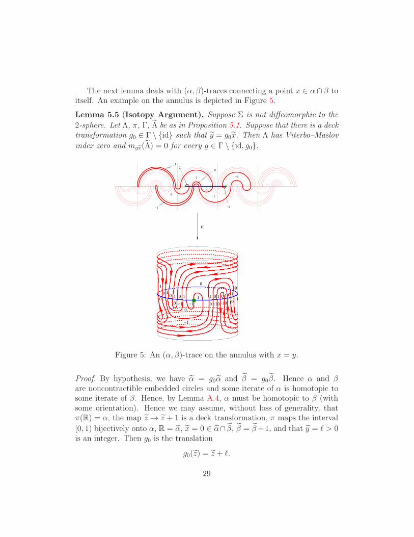
The next lemma deals with (α, β)-traces connecting a point x ∈ α ∩ β toitself. An example on the annulus is depicted in Figure 5.
Lemma 5.5 (Isotopy Argument). Suppose Σ is not diffeomorphic to the
2-sphere. Let Λ, π, Γ, Λ be as in Proposition 5.1. Suppose that there is a decktransformation g0 ∈ Γ \ id such that y = g0x. Then Λ has Viterbo–Maslov
index zero and mgex(Λ) = 0 for every g ∈ Γ \ id, g0.
−2
−10−1
0
0
1−1
1
0
−1
0
2
−1
1
0
0
−1
0
0
−1
π
0
1
0
111
−10
1
0
−1
10
1
0 1 0 0 0
−1
Figure 5: An (α, β)-trace on the annulus with x = y.
Proof. By hypothesis, we have α = g0α and β = g0β. Hence α and βare noncontractible embedded circles and some iterate of α is homotopic tosome iterate of β. Hence, by Lemma A.4, α must be homotopic to β (withsome orientation). Hence we may assume, without loss of generality, thatπ(R) = α, the map z 7→ z + 1 is a deck transformation, π maps the interval
[0, 1) bijectively onto α, R = α, x = 0 ∈ α∩ β, β = β+1, and that y = ℓ > 0is an integer. Then g0 is the translation
g0(z) = z + ℓ.
29

Let A := [0, ℓ] ⊂ α and let B ⊂ β be the arc connecting 0 to ℓ. Then, for
z ∈ C \ (A ∪ B), the integer w(z) is the winding number of A− B about z.Define the projection π0 : C → C by
π0(z) := e2πiez/ℓ,
denote α0 := π0(α) = S1 and β0 := π(β), and let Λ0 = (1, 1,w0) be theinduced (α0, β0)-trace in C with w0(z) :=
∑ez∈π−1(z) w(z). Then Λ0 satisfies
the conditions of Step 8, Case 3 in the proof of Proposition 4.1 and itsboundary is given by να0 = ∂w0|α0\β0 ≡ 1 and νβ0 = ∂w0|β0\α0 ≡ 1. Hence
Λ0 and Λ have Viterbo–Maslov index zero.It remains to prove that mgex(Λ) = 0 for every g ∈ Γ \ id, g0. To see
this we use the fact that the embedded loops α and β are homotopic withfixed endpoint x. Hence, by a Theorem of Epstein, they are isotopic withfixed basepoint x (see [8, Theorem 4.1]). Thus there exists a smooth mapf : R/Z× [0, 1] → Σ such that
f(s, 0) ∈ α, f(s, 1) ∈ β, f(0, t) = x,
for all s ∈ R/Z and t ∈ [0, 1], and the map R/Z → Σ : s 7→ f(s, t) is anembedding for every t ∈ [0, 1]. Lift this homotopy to the universal cover to
obtain a map f : R× [0, 1] → C such that π f = f and
f(s, 0) ∈ [0, 1], f(s, 1) ∈ B1, f(0, t) = x, f(s+ k, t) = f(s, t) + k
for all s, t ∈ [0, 1] and k ∈ Z. Here B1 ⊂ B denotes the arc in B from 0 to 1.Since the map R/Z → Σ : s 7→ f(s, t) is injective for every t, we have
gx /∈ x, x+ 1, . . . , x+ ℓ =⇒ gx /∈ f([0, ℓ]× [0, 1])
for every every g ∈ Γ. Now choose a smooth map u : D → C withΛeu = Λ (see Theorem 2.4). Define the homotopy Feu : [0, ℓ] × [0, 1] → C
by Feu(s, t) := u(− cos(πs/ℓ), t sin(πs/ℓ)). Then, by Theorem 2.4, Feu is ho-
motopic to f |[0,ℓ]×[0,1] subject to the boundary conditions f(s, 0) ∈ α = R,
f(s, 1) ∈ β, f(0, t) = x, f(ℓ, t) = y. Hence, for every z ∈ C\ (α∪ β), we have
w(z) = deg(u, z) = deg(Feu, z) = deg(f , z).
In particular, choosing z near gx, we find mgex(Λ) = 4 deg(f , gx) = 0 forevery g ∈ Γ that is not one of the translations z 7→ z + k for k = 0, 1, . . . , ℓ.This proves the assertion in the case ℓ = 1.
30

If ℓ > 1 it remains to prove mk(Λ) = 0 for k = 1, . . . , ℓ− 1. To see this,
let A1 := [0, 1], B1 ⊂ B be the arc from 0 to 1, w1(z) be the winding number
of A1 − B1 about z ∈ C \ (A1 ∪ B1), and define Λ1 := (0, 1, w1). Then, by
what we have already proved, the (α, β)-trace Λ1 satisfies mgex(Λ1) = 0 forevery g ∈ Γ other than the translations by 0 or 1. In particular, we havemj(Λ1) = 0 for every j ∈ Z \ 0, 1 and also m0(Λ1)+m1(Λ1) = 2µ(Λ1) = 0.
Since w(z) =∑ℓ−1
j=0 w1(z − j) for z ∈ C \ (A ∪ B), we obtain
mk(Λ) =
ℓ−1∑
j=0
mk−j(Λ1) = 0
for every k ∈ Z \ 0, ℓ. This proves Lemma 5.5.
The next example shows that Lemma 5.4 cannot be strengthened to assertthe identity mgex(Λ) = 0 for every g ∈ Γ with gx, gy /∈ A ∪ B.
Example 5.6. Figure 6 depicts an (α, β)-trace Λ = (x, y,w) on the annulusΣ = C/Z that has Viterbo–Maslov index one and satisfies the arc condition.
The lift satisfies mex(Λ) = −3, mex+1(Λ) = 4, mey(Λ) = 5, and mey−1(Λ) = −4.Thus mx(Λ) = my(Λ) = 1.
π
~
x
~~x
~x+1~ ~x~ x+1~2
y1
−1
y
−1
1
1
1
y−1
−1
y
2
y−1
0
Figure 6: An (α, β)-trace on the annulus satisfying the arc condition.
31

Proof of Proposition 5.1. The proof has five steps.
Step 1. Let A, B ⊂ C be as in Lemma 5.3 and let g ∈ Γ such that
gx ∈ A \ B, gy /∈ A ∪ B.
(An example is depicted in Figure 7.) Then (21) holds.
−1
π
131
01
0
−1
−1
−2−1
~gx~g y~x~
−1
1
1
y
Figure 7: An (α, β)-trace on the torus not satisfying the arc condition.
The proof is a refinement of the winding number comparison argument inLemma 5.4. Since gx /∈ B we have g 6= id and, since x, gx ∈ A ⊂ α, itfollows that α is a noncontractible embedded circle. Hence we may choosethe universal covering π : C → Σ and the lifts α, β, Λ such that π(R) = α,the map z 7→ z + 1 is a deck transformation, the projection π maps theinterval [0, 1) bijectively onto α, and
α = R, x = 0 ∈ α ∩ β, y > 0.
By hypothesis and Lemma 5.3 there is an integer k such that
0 < k < y, gx = k, g−1y = y − k.
Thus g is the deck transformation z 7→ z + k.
32

Since gx /∈ B and gy /∈ B it follows from Lemma 5.3 that g−1y /∈ B andg−1x /∈ B and hence, again by Lemma 5.3, we have
B ∩ gB = B ∩ g−1B = ∅.
With γeα and γeβ chosen as in Lemma 5.3, this implies
γeβ · (γeβ − k) = (γeβ + k) · γeβ = 0. (26)
Since k,−k, y + k, y − k /∈ B, there exists a constant ε > 0 such that
−ε ≤ t ≤ ε =⇒ k + it, −k + it, y − k + it, y + k + it /∈ B.
The paths gγeα ± iε and gγeβ ± iε both connect the point gx± iε to gy ± iε.
Likewise, the paths g−1γeα±iε and g−1γeβ±iε both connect the point g−1x±iε
to g−1y ± iε. Hence
w(gy ± iε)− w(gx± iε) = (γeα − γeβ) · (gγeα ± iε)
= (γeα − γeβ) · (γeα + k ± iε)
= (γeα + k ± iε) · γeβ
= γeα · (γeβ − k ∓ iε)
= (γeα − γeβ) · (γeβ − k ∓ iε)
= (γeα − γeβ) · (g−1γeβ ∓ iε)
= w(g−1y ∓ iε)− w(g−1x∓ iε).
Here the last but one equation follows from (26). Thus we have proved
w(gx+ iε) + w(g−1y − iε) = w(g−1x− iε) + w(gy + iε),
w(gx− iε) + w(g−1y + iε) = w(g−1x+ iε) + w(gy − iε).(27)
Since
mgex(Λ) = 2w(gx+ iε) + 2w(gx− iε),
mgey(Λ) = 2w(gy + iε) + 2w(gy − iε),
mg−1ex(Λ) = 2w(g−1x+ iε) + 2w(g−1x− iε),
mg−1ey(Λ) = 2w(g−1y + iε) + 2w(g−1y − iε),
Step 1 follows by taking the sum of the two equations in (27).
33

Step 2. Let A, B ⊂ C be as in Lemma 5.3 and let g ∈ Γ. Suppose thateither gx, gy /∈ A or gx, gy /∈ B. Then (21) holds.
If gx, gy /∈ A ∪ B the assertion follows from Lemma 5.4. If gx ∈ A \ B and
gy /∈ A∪B the assertion follows from Step 1. If gx /∈ A∪B and gy ∈ A\B theassertion follows from Step 1 by interchanging x and y. Namely, (21) holds
for Λ if and only if it holds for the (α, β)-trace −Λ := (y, x,−w). This covers
the case gx, gy /∈ B. If gx, gy /∈ A the assertion follows by interchanging Aand B. Namely, (21) holds for Λ if and only if it holds for the (β, α)-trace
Λ∗ := (x, y,−w). This proves Step 2.
Step 3. Let A, B ⊂ C be as in Lemma 5.3 and let g ∈ Γ such that
gx ∈ A \ B, gy ∈ B \ A.
(An example is depicted in Figure 8.) Then the cancellation formula (20)holds for g and g−1.
3
−1−2
1
0
1
−1
−1
−1−2
010
1
2
010
−1
π
101
0−1 1
−1
Figure 8: An (α, β)-trace on the annulus with gx ∈ A and gy ∈ B.
Since gx /∈ B (and gy /∈ A) we have g 6= id and, since x, gx ∈ A ⊂ α
and y, gy ∈ B ⊂ β, it follows that gα = α and gβ = β. Hence α and β arenoncontractible embedded circles and some iterate of α is homotopic to someiterate of β. So α is homotopic to β (with some orientation), by Lemma A.4.
34

Choose the universal covering π : C → Σ and the lifts α, β, Λ such thatπ(R) = α, the map z 7→ z + 1 is a deck transformation, π maps the interval[0, 1) bijectively onto α, and
α = R, x = 0 ∈ α ∩ β, y > 0.
Thus A = [0, y] is the arc in α from 0 to y and B is the arc in β from 0 to y.Moreover, since α is homotopic to β, we have
β = β + 1
and the arc in β from 0 to 1 is a fundamental domain for β. Since gα = α,the deck transformation g is given by z 7→ z + ℓ for some integer ℓ. Sincegx ∈ A \ B and gy ∈ B, we have g−1y /∈ B and g−1x ∈ B by Lemma 5.3.Hence
0 < ℓ < y, ℓ /∈ B, y + ℓ ∈ B, y − ℓ /∈ B, −ℓ ∈ B.
This shows that, walking along β from 0 to y (traversing B) one encounterssome negative integer and therefore no positive integers. Hence
A ∩ Z =0, 1, 2, · · · , k eA
, B ∩ Z =
0,−1,−2, · · · ,−k eB
,
where k eA is the number of fundamental domains of α contained in A and k eB
is the number of fundamental domains of β contained in B (see Figure 8).
For 0 ≤ k ≤ k eA let Ak ⊂ α and Bk ⊂ β be the arcs from 0 to y− k. Thus Ak
is obtained from A by removing k fundamental domains at the end, while Bk
is obtained from B by attaching k fundamental domains at the end. Considerthe (α, β)-trace
Λk := (0, y − k, wk), ∂Λk := (0, y − k, Ak, Bk),
where wk : C \ (Ak ∪ Bk) → Z is the winding number of Ak − Bk. Then
Bk ∩ Z =0,−1,−2, · · · ,−k eB − k
and Λ0 = Λ. We prove that, for each k, the (α, β)-trace Λk satisfies
mj(Λk) +mey−k−j(Λk) = 0 ∀ j ∈ Z \ 0. (28)
If y is an integer, then (28) follows from Lemma 5.5. Hence we may assumethat y is not an integer.
35
We prove equation (28) by reverse induction on k. First let k = k eA. Then
we have j, y − k + j /∈ Ak for every j ∈ N. Hence it follows from Step 2 that
mj(Λk) +mey−k−j(Λk) = m−j(Λk) +mey−k+j(Λ) ∀ j ∈ N. (29)
Thus we can apply Lemma 5.2 to the projection of Λk to the quotient C/Z.
Hence Λk satisfies (28).Now fix an integer k ∈ 0, 1, . . . , k eA − 1 and suppose, by induction, that
Λk+1 satisfies (28). Denote by A′ ⊂ α and B′ ⊂ β the arcs from y − k − 1
to 1, and by A′′ ⊂ α and B′′ ⊂ β the arcs from 1 to y − k. Then Λk is thecatenation of the (α, β)-traces
Λk+1 := (0, y − k − 1, wk+1), ∂Λk+1 = (0, y − k − 1, Ak+1, Bk+1),
Λ′ := (y − k − 1, 1, w′), ∂Λ′ = (y − k − 1, 1, A′, B′),
Λ′′ := (1, y − k, w′′), ∂Λ′′ = (1, y − k, A′′, B′′).
Here w′(z) is the winding number of the loop A′− B′ about z ∈ C \ (A′∪ B′)
and simiarly for w′′. Note that Λ′′ is the shift of Λk+1 by 1. The catenationof Λk+1 and Λ′ is the (α, β)-trace from 0 to 1. Hence it has Viterbo–Maslovindex zero, by Lemma 5.5, and satisfies
mj(Λk+1) +mj(Λ′) = 0 ∀j ∈ Z \ 0, 1. (30)
Since the catenation of Λ′ and Λ′′ is the (α, β)-trace from y− k− 1 to y− k,it also has Viterbo–Maslov index zero and satisfies
mey−k−j(Λ′) +mey−k−j(Λ
′′) = 0 ∀j ∈ Z \ 0, 1. (31)
Moreover, by the induction hypothesis, we have
mj(Λk+1) +mey−k−1−j(Λk+1) = 0 ∀j ∈ Z \ 0. (32)
Combining the equations (30), (31), (32) we find that, for j ∈ Z \ 0, 1,
mj(Λk) +mey−k−j(Λk) = mj(Λk+1) +mj(Λ′) +mj(Λ
′′)
+mey−k−j(Λk+1) +mey−k−j(Λ′) +mey−k−j(Λ
′′)
= mj(Λk+1) +mj(Λ′)
+mey−k−j(Λ′) +mey−k−j(Λ
′′)
+mj−1(Λk+1) +mey−k−j(Λk+1)
= 0.
36

For j = 1 we obtain
m1(Λk) +mey−k−1(Λk) = m1(Λk+1) +m1(Λ′) +m1(Λ
′′)
+mey−k−1(Λk+1) +mey−k−1(Λ′) +mey−k−1(Λ
′′)
= m1(Λk+1) +mey−k−2(Λk+1)
+m0(Λk+1) +mey−k−1(Λk+1)
+mey−k−1(Λ′) +m1(Λ
′)
= 2µ(Λk+1) + 2µ(Λ′)
= 0.
Here the last but one equation follows from equation (32) and Proposition 4.1,
and the last equation follows from Lemma 5.5. Hence Λk satisfies (28). Thiscompletes the induction argument for the proof of Step 3.
Step 4. Let A, B ⊂ C be as in Lemma 5.3 and let g ∈ Γ such that
gx ∈ A ∩ B, gy /∈ A ∪ B.
Then the cancellation formula (20) holds for g and g−1.
The proof is by induction and catenation based on Step 2 and Lemma 5.5.Since gy /∈ A ∪ B we have g 6= id. Since gx ∈ A ∩ B we have α = gαand β = gβ. Hence α and β are noncontractible embedded circles, and theyare homotopic (with some orientation) by Lemma A.4. Thus we may choose
π : C → Σ, α, β, Λ as in Step 3. By hypothesis there is an integer k ∈ A∩ B.Hence A and B do not contain any negative integers. Choose k eA, k eB ∈ N
such that
A ∩ Z =0, 1, . . . , k eA
, B ∩ Z =
0, 1, . . . , k eB
.
Assume without loss of generality that
k eA ≤ k eB.
For 0 ≤ k ≤ k eA denote by Ak ⊂ A and Bk ⊂ B the arcs from 0 to y − k and
consider the (α, β)-trace
Λk := (0, y − k, wk), ∂Λk := (0, y − k, Ak, Bk).
37

In this caseBk ∩ Z = 0, 1, . . . , k eB − k.
As in Step 3, it follows by reverse induction on k that Λk satisfies (28) forevery k. We assume again that y is not an integer. (Otherwise (28) follows
from Lemma 5.5). If k = k eA then j, y − k + j /∈ Ak for every j ∈ N, hence it
follows from Step 2 that Λk satisfies (29), and hence it follows from Lemma 5.2
for the projection of Λk to the annulus C/Z that Λk also satisfies (28). Theinduction step is verbatim the same as in Step 3 and will be omitted. Thisproves Step 4.
Step 5. We prove Proposition 5.1.
If both points gx, gy are contained in A (or in B) then g = id by Lemma 5.3,and in this case equation (21) is a tautology. If both points gx, gy are not
contained in A∪ B, equation (21) has been established in Lemma 5.4. More-
over, we can interchange x and y or A and B as in the proof of Step 2. ThusSteps 1 and 4 cover the case where precisely one of the points gx, gy is con-tained in A ∪ B while Step 3 covers the case where g 6= id and both pointsgx, gy are contained in A∪ B. This shows that equation (21) holds for everyg ∈ Γ \ id. Hence, by Lemma 5.2, the cancellation formula (20) holds forevery g ∈ Γ \ id. This proves Proposition 5.1.
Proof of Theorem 3.4 in the Non Simply Connected Case. Choose a univer-sal covering π : C → Σ and let Γ, α, β, and Λ = (x, y, w) be as in Proposi-tion 5.1. Then
mx(Λ) +my(Λ)−mex(Λ)−mey(Λ) =∑
g 6=id
(mgex(Λ) +mg−1ey(Λ)
)= 0.
Here the last equation follows from the cancellation formula in Proposi-tion 5.1. Hence, by Proposition 4.1, we have
µ(Λ) = µ(Λ) =mex(Λ) +mey(Λ)
2=mx(Λ) +my(Λ)
2.
This proves the trace formula in the case where Σ is not simply connected.
38

II. Combinatorial Lunes
6 Lunes and Traces
We denote the universal covering of Σ by
π : Σ → Σ
and, when Σ is not diffeomorphic to the 2-sphere, we assume Σ = C.
Definition 6.1 (Smooth Lunes). Assume (H). A smooth (α, β)-lune isan orientation preserving immersion u : D → Σ such that
u(D ∩ R) ⊂ α, u(D ∩ S1) ⊂ β,
Three examples of smooth lunes are depicted in Figure 9. Two lunes aresaid to be equivalent iff there is an orientation preserving diffeomorphismϕ : D → D such that
ϕ(−1) = −1, ϕ(1) = 1, u′ = u ϕ.
The equivalence class of u is denoted by [u]. That u is an immersion meansthat u is smooth and du is injective in all of D, even at the corners ±1.The set u(D ∩ R) is called the bottom boundary of the lune, and the setu(D ∩ S1) is called the top boundary. The points
x = u(−1), y = u(1)
are called respectively the left and right endpoints of the lune. The locallyconstant function
Σ \ u(∂D) → N : z 7→ #u−1(z)
is called the counting function of the lune. (This function is locallyconstant because a proper local homeomorphism is a covering projection.)A smooth lune is said to be embedded iff the map u is injective. Thesenotions depend only on the equivalence class [u] of the smooth lune u.
Our objective is to characterize smooth lunes in terms of their boundarybehavior, i.e. to say when a pair of immersions uα : (D ∩ R,−1, 1) → (α, x, y)and uβ : (D ∩ S1,−1, 1) → (β, x, y) extends to a smooth (α, β)-lune u. Recallthe following definitions and theorems from Part I.
39

1
2
1
2
1
1
1 21 2
3
0
0
1
2
12
00
1212
3
0
1
0
45
4
4
3
211
4
3
1
1
2
2
1
1 0
3 232
Figure 9: Three lunes.
40

Definition 6.2 (Traces). Assume (H). An (α, β)-trace is a triple
Λ = (x, y,w)
such that x, y ∈ α ∩ β and w : Σ \ (α ∪ β) → Z is a locally constant functionsuch that there exists a smooth map u : D → Σ satisfying
u(D ∩ R) ⊂ α, u(D ∩ S1) ⊂ β, (33)
u(−1) = x, u(1) = y, (34)
w(z) = deg(u, z), z ∈ Σ \ (α ∪ β). (35)
The (α, β)-trace associated to a smooth map u : D → Σ satisfying (33) isdenoted by Λu.
The boundary of an (α, β)-trace Λ = (x, y,w) is the triple
∂Λ := (x, y, ∂w).
Here∂w : (α \ β) ∪ (β \ α) → Z
is the locally constant function that assigns to z ∈ α\β the value of w slightlyto the left of α minus the value of w slightly to the right of α near z, andto z ∈ β \ α the value of w slightly to the right of β minus the value of wslightly to the left of β near z.
In Lemma 2.3 above it was shown that, if Λ = (x, y,w) is the (α, β)-traceof a smooth map u : D → Σ that satisfies (33), then ∂Λu = (x, y, ν), wherethe function ν := ∂w : (α \ β) ∪ (β \ α) → Z is given by
ν(z) =
deg(u
∣∣∂D∩R
: ∂D ∩ R → α, z), for z ∈ α \ β,− deg(u
∣∣∂D∩S1 : ∂D ∩ S1 → β, z), for z ∈ β \ α.
(36)
Here we orient the one-manifolds D∩R and D∩S1 from −1 to +1. Moreover,in Theorem 2.4 above it was shown that the homotopy class of a smooth mapu : D → Σ satisfying the boundary condition (33) is uniquely determined byits trace Λu = (x, y,w). If Σ is not diffeomorphic to the 2-sphere then itsuniversal cover is diffeomorphic to the 2-plane. In this situation it was alsoshown in Theorem 2.4 that the homotopy class of u and the degree functionw are uniquely determined by the triple ∂Λu = (x, y, ν).
41

Remark 6.3 (The Viterbo–Maslov index). Let Λ = (x, y,w) be an(α, β)-trace and denote by µ(Λ) its Viterbo–Maslov index as defined in 3.1above (see also [39]). For z ∈ α∩β let mz(Λ) be the sum of the four values ofthe function w encountered when walking along a small circle surrounding z.In Theorem 3.4 it was shown that the Viterbo–Maslov index of Λ is given bythe trace formula
µ(Λ) =mx(Λ) +my(Λ)
2. (37)
Let Λ′ = (y, z,w′) be another (α, β)-trace. The catenation of Λ and Λ′ isdefined by
Λ#Λ′ := (x, z,w + w′).
It is again an (α, β)-trace and has Viterbo–Maslov index
µ(Λ#Λ′) = µ(Λ) + µ(Λ′). (38)
For a proof see [39, 30].
Definition 6.4 (Arc Condition). Let Λ = (x, y,w) be an (α, β)-trace and
να := ∂w|α\β , νβ := −∂w|β\α.
Λ is said to satisfy the arc condition if
x 6= y, min |να| = min |νβ| = 0. (39)
When Λ satisfies the arc condition there are arcs A ⊂ α and B ⊂ β from xto y such that
να(z) =
±1, if z ∈ A,0, if z ∈ α \ A,
νβ(z) =
±1, if z ∈ B,0, if z ∈ β \B.
(40)
Here the plus sign is chosen iff the orientation of A from x to y agrees withthat of α, respectively the orientation of B from x to y agrees with that of β.In this situation the quadruple (x, y, A,B) and the triple (x, y, ∂w) determineone another and we also write
∂Λ = (x, y, A,B)
for the boundary of Λ. When u : D → Σ is a smooth map satisfying (33)and Λu = (x, y,w) satisfies the arc condition and ∂Λu = (x, y, A,B) then thepath s 7→ u(− cos(πs), 0) is homotopic in α to a path traversing A and thepath s 7→ u(− cos(πs), sin(πs)) is homotopic in β to a path traversing B.
42

Theorem 6.5. Assume (H). If u : D → Σ is a smooth (α, β)-lune then its(α, β)-trace Λu satisfies the arc condition.
Proof. See Section 7 page 55.
Definition 6.6 (Combinatorial Lunes). Assume (H). A combinatorial(α, β)-lune is an (α, β)-trace Λ = (x, y,w) with boundary ∂Λ =: (x, y, A,B)that satisfies the arc condition and the following.
(I) w(z) ≥ 0 for every z ∈ Σ \ (α ∪ β).
(II) The intersection index of A and B at x is +1 and at y is −1.
(III) w(z) ∈ 0, 1 for z sufficiently close to x or y.
Condition (II) says that the angle from A to B at x is between zero and πand the angle from B to A at y is also between zero and π.
1
1
2−1
2
−1
1 1 1
1
Figure 10: (α, β)-traces which satisfy the arc condition but are not lunes.
Theorem 6.7 (Existence). Assume (H) and let Λ = (x, y,w) be an (α, β)-trace. Consider the following three conditions.
(i) There exists a smooth (α, β)-lune u such that Λu = Λ.
(ii) w ≥ 0 and µ(Λ) = 1.
(iii) Λ is a combinatorial (α, β)-lune.
Then (i) =⇒ (ii) ⇐⇒ (iii). If Σ is simply connected then all three conditionsare equivalent.
Proof. See Section 8 page 63.
43

Theorem 6.8 (Uniqueness). Assume (H). If two smooth (α, β)-lunes havethe same trace then they are equivalent.
Proof. See Section 8 page 63.
Corollary 6.9. Assume (H) and let
Λ = (x, y,w)
be an (α, β)-trace. Choose a universal covering π : Σ → Σ, a point
x ∈ π−1(x),
and lifts α and β of α and β such that
x ∈ α ∩ β.
LetΛ = (x, y, w)
be the lift of Λ to the universal cover.
(i) If Λ is a combinatorial (α, β)-lune then Λ is a combinatorial (α, β)-lune.
(ii) Λ is a combinatorial (α, β)-lune if and only if there exists a smooth(α, β)-lune u such that Λu = Λ.
Proof. Lifting defines a one-to-one correspondence between smooth (α, β)-
lunes with trace Λ and smooth (α, β)-lunes with trace Λ. Hence the assertionsfollow from Theorem 6.7.
Remark 6.10. Assume (H) and let Λ be an (α, β)-trace. We conjecturethat the three conditions in Theorem 6.7 are equivalent, even when Σ is notsimply connected, i.e.
If Λ is a combinatorial (α, β)-lunethen there exists a smooth (α, β)-lune u such that Λ = Λu.
Theorem 6.7 shows that this conjecture is equivalent to the following.
If Λ is a combinatorial (α, β)-lune
then Λ is a combinatorial (α, β)-lune.
The hard part is to prove that Λ satisfies (I), i.e. that the winding numbersare nonnegative.
44

Remark 6.11. Assume (H). Corollary 6.9 and Theorem 6.8 suggest thefollowing algorithm for finding a smooth (α, β)-lune.
1. Fix two points x, y ∈ α ∩ β with opposite intersection indices, and twooriented embedded arcs A ⊂ α and B ⊂ β from x to y so that (II) holds.
2. If A is not homotopic to B with fixed endpoints discard this pair.1 Oth-erwise (x, y, A,B) is the boundary of an (α, β)-trace Λ = (x, y,w) satisfyingthe arc condition and (II) (for a suitable function w to be chosen below).
3a. If Σ is diffeomorphic to the 2-sphere let w : Σ \ (A ∪ B) → Z be thewinding number of the loop A − B in Σ \ z0, where z0 ∈ α \ A is chosenclose to x. Check if w satisfies (I) and (III). If yes, then Λ = (x, y,w) is acombinatorial (α, β)-lune and hence, by Theorems 6.7 and 6.8, gives rise toa smooth (α, β)-lune u, unique up to isotopy.
3b. If Σ is not diffeomorphic to the 2-sphere choose lifts A of A and B of Bto a universal covering π : C → Σ connecting x and y and let
w : C \ (A ∪ B) → Z
be the winding number of A − B. Check if w satisfies (I) and (III). If yes,
then Λ := (x, y, w) is a combinatorial (α, β)-lune and hence, by Theorem 6.7,gives rise to a smooth (α, β)-lune u such that
Λu = Λ := (x, y,w), w(z) :=∑
ez∈π−1(z)
w(z).
By Theorem 6.8, the (α, β)-lune u is uniquely determined by Λ up to isotopy.
Proposition 6.12. Assume (H) and let Λ = (x, y,w) be an (α, β)-trace thatsatisfies the arc condition and let ∂Λ =: (x, y, A,B). Let S be a connectedcomponent of Σ \ (A∪B) such that w|S 6≡ 0. Then S is diffeomorphic to theopen unit disc in C.
Proof. By Definition 6.2, there is a smooth map u : D → Σ satisfying (33)such that Λu = Λ. By a homotopy argument we may assume, without lossof generality, that u(D ∩ R) = A and u(D ∩ S1) = B. Let S be a connectedcomponent of Σ \ (A ∪ B) such that w does not vanish on S. We prove intwo steps that S is diffeomorphic to the open unit disc in C.
1 This problem is solvable via Dehn’s algorithm. See the wikipedia article
Small Cancellation Theory and the references cited therein.
45

Step 1. If S is not diffeomorphic to the open unit disc in C then there isan embedded loop γ : R/Z → S and a loop γ′ : R/Z → Σ with intersectionnumber γ · γ′ = 1.
If S has positive genus there are in fact two embedded loops in S withintersection number one. If S has genus zero but is not diffeomorphic to thedisc it is diffeomorphic to a multiply connected subset of C, i.e. a disc withat least one hole cut out. Let γ : R/Z → S be an embedded loop encirclingone of the holes and choose an arc in S which connects two boundary pointsand has intersection number one with γ. (For an elegant construction ofsuch a loop in the case of an open subset of C see Ahlfors [3].) Since Σ \S isconnected the arc can be completed to a loop in Σ which still has intersectionnumber one with γ. This proves Step 1.
Step 2. S is diffeomorphic to the open unit disc in C.
Assume, by contradiction, that this is false and choose γ and γ′ as in Step 1.By transversality theory we may assume that u is transverse to γ. SinceC := γ(R/Z) is disjoint from u(∂D) = A ∪ B it follows that Γ := u−1(C)is a disjoint union of embedded circles in ∆ := u−1(S) ⊂ D. Orient Γ suchthat the degree of u|Γ : Γ → C agrees with the degree of u|∆ : ∆ → S.More precisely, let z ∈ Γ and t ∈ R/Z such that u(z) = γ(t). Call a nonzerotangent vector z ∈ TzΓ positive if the vectors γ(t), du(z)iz form a positivelyoriented basis of Tu(z)Σ. Then, if z ∈ Γ is a regular point of both u|∆ : ∆ → Sand u|Γ : Γ → C, the linear map du(z) : C → Tu(z)Σ has the same sign asits restriction du(z) : TzΓ → Tu(z)C. Thus u|Γ : Γ → C has nonzero degree.Choose a connected component Γ0 of Γ such that u|Γ0 : Γ0 → C has degreed 6= 0. Since Γ0 is a loop in D it follows that the d-fold iterate of γ iscontractible. Hence γ is contractible by A.3 in Appendix A. This provesStep 2 and Proposition 6.12.
7 Arcs
In this section we prove Theorem 6.5. The first step is to prove the arccondition under the hypothesis that α and β are not contractible (Propo-sition 7.1). The second step is to characterize embedded lunes in terms oftheir traces (Proposition 7.4). The third step is to prove the arc conditionfor lunes in the two-sphere (Proposition 7.7).
46

Proposition 7.1. Assume (H), suppose Σ is not simply connected, andchoose a universal covering π : C → Σ. Let Λ = (x, y,w) be an (α, β)-traceand denote
να := ∂w|α\β , νβ := −∂w|β\α.
Choose lifts α, β, and Λ = (x, y, w) of α, β, and Λ such that Λ is an (α, β)-
trace. Thus x, y ∈ α ∩ β and the path from x to y in α (respecively β)determined by ∂w is the lift of the path from x to y in α (respectively β)determined by ∂w. Assume
w ≥ 0, w 6≡ 0.
Then the following holds
(i) If α is a noncontractible embedded circle then there exists an oriented arcA ⊂ α from x to y (equal to x in the case x = y) such that
να(z) =
±1, for z ∈ A \ β,0, for z ∈ α \ (A ∪ β).
(41)
Here the plus sign is chosen if and only if the orientations of A and α agree.If β is a noncontractible embedded circle the same holds for νβ.
(ii) If α and β are both noncontractible embedded circles then Λ satisfies thearc condition.
Proof. We prove (i). The universal covering π : C → Σ and the lifts α, β,
and Λ = (x, y, w) can be chosen such that
α = R, x = 0, y = a ≥ 0, π(z + 1) = π(z),
and π maps the interval [0, 1) bijectively onto α. Denote by
B ⊂ β
the closure of the support of
νeβ := −∂w|eβ\eα.
If β is noncontractible then B is the unique arc in β from 0 to a. If β iscontractible then β ⊂ C is an embedded circle and B is either an arc in β
47

ca
1 2
13
0b
Figure 11: The lift of an (α, β)-trace with w ≥ 0.
from 0 to a or is equal to β. We must prove that A := π([0, a]) is an arc or,equivalently, that a < 1.
Let Γ be the set of connected components γ of B ∩ (R× [0,∞)) such thatthe function w is zero on one side of γ and positive on the other. If γ ∈ Γ,neither end point of γ can lie in the open interval (0, a) since the functionw is at least one above this interval. We claim that there exists a connectedcomponent γ ∈ Γ whose endpoints b and c satisfy
b ≤ 0 ≤ a ≤ c, ∂γ = b, c. (42)
(See Figure 11.) To see this walk slightly above the real axis towards zero,
starting at −∞. Just before the first crossing b1 with B turn left and followthe arc in B until it intersects the real axis again at c1. The two intersectionsb1 and c1 are the endpoints of an element γ1 of Γ. Obviously b1 ≤ 0 and,as noted above, c1 cannot lie in the interval (0, a). For the same reason c1cannot be equal to zero. Hence either c1 < 0 or c1 ≥ a. In the latter case γ1is the required arc γ. In the former case we continue walking towards zeroalong the real axis until the next intersection with B and repeat the aboveprocedure. Because the set of intersection points of B with α = R is finitethe process must terminate after finitely many steps. Thus we have provedthe existence of an arc γ ∈ Γ satisfying (42).
Assume thatc ≥ b+ 1.
If c = b + 1 then c ∈ β ∩ (β + 1) and hence β = β + 1. It follows that the
intersection numbers of R and β at b and c agree. But this contradicts the
48

fact that b and c are the endpoints of an arc in β contained in the closedupper halfplane. Thus we have c > b + 1. When this holds the arc γ andits translate γ + 1 must intersect and their intersection does not contain theendpoints b and c. We denote by ζ ∈ γ \ b, c the first point in γ + 1 weencounter when walking along γ from b to c. Let
U0 ⊂ β, U1 ⊂ β + 1
be sufficiently small connected open neighborhoods of ζ , so that π : U0 → βand π : U1 → β are embeddings and their images agree. Thus
π(U0) = π(U1) ⊂ β
is an open neighborhood of z := π(ζ) in β. Hence it follows from a liftingargument that U0 = U1 ⊂ γ + 1 and this contradicts our choice of ζ . Thiscontradiction shows that our hypothesis c ≥ b + 1 must have been wrong.Thus we have proved that
b ≤ 0 ≤ a ≤ c < b+ 1 ≤ 1.
Hence 0 ≤ a < 1 and so A = π([0, a]) is an arc, as claimed. In the case a = 0we obtain the trivial arc from x = y to itself. This proves (i).
We prove (ii). Assume that α and β are noncontractible embedded circles.Then it follows from (i) that there exist oriented arcs A ⊂ α and B ⊂ β fromx to y such that να and νβ are given by (40). If x = y it follows also from (i)that A = B = x, hence
νeα ≡ 0, νeβ ≡ 0,
and hence w ≡ 0, in contradiction to our hypothesis. Thus x 6= y and so Λsatisfies the arc condition. This proves (ii) and Proposition 7.1.
Example 7.2. Let α ⊂ Σ be a noncontractible embedded circle and β ⊂ Σbe a contractible embedded circle intersecting α transversally. Suppose β isoriented as the boundary of an embedded disc ∆ ⊂ Σ. Let
x = y ∈ α ∩ β, να ≡ 0, νβ ≡ 1,
and define
w(z) :=
1, for z ∈ ∆ \ (α ∪ β),0, for z ∈ Σ \ (∆ ∪ α ∪ β).
Then Λ = (x, y, να, νβ,w) is an (α, β)-trace that satisfies the hypotheses ofProposition 7.1 (i) with x = y and A = x.
49

Definition 7.3. An (α, β)-trace Λ = (x, y,w) is called primitive if it satis-fies the arc condition with boundary ∂Λ =: (x, y, A,B) and
A ∩ β = α ∩ B = x, y.
A smooth (α, β)-lune u is called primitive if its (α, β)-trace Λu is primitive.It is called embedded if u : D → Σ is injective.
The next proposition is the special case of Theorems 6.7 and 6.8 for em-bedded lunes. It shows that isotopy classes of primitive smooth (α, β)-lunesare in one-to-one correspondence with the simply connected components ofΣ\(α∪β) with two corners. We will also call such a component a primitive(α, β)-lune.
Proposition 7.4 (Embedded lunes). Assume (H) and let Λ = (x, y,w)be an (α, β)-trace. The following are equivalent.
(i) Λ is a combinatorial lune and its boundary ∂Λ = (x, y, A,B) satisfies
A ∩ B = x, y.
(ii) There exists an embedded (α, β)-lune u such that Λu = Λ.
If Λ satisfies (i) then any two smooth (α, β)-lunes u and v with Λu = Λv = Λare equivalent.
Proof. We prove that (ii) implies (i). Let u : D → Σ be an embedded (α, β)-lune with Λu = Λ. Then u|D∩R : D ∩ R → α and u|D∩S1 : D ∩ S1 → β areembeddings. Hence Λ satisfies the arc condition and ∂Λ = (x, y, A,B) withA = u(D ∩ R) and B = u(D ∩ S1). Since w is the counting function of u ittakes only the values zero and one. If z ∈ A∩B then u−1(z) contains a singlepoint which must lie in D ∩ R and D ∩ S1, hence is either −1 or +1, and soz = x or z = y. The assertion about the intersection indices follows from thefact that u is an immersion. Thus we have proved that (ii) implies (i).
We prove that (i) implies (ii). This relies on the following.
Claim. Let Λ = (x, y,w) be an (α, β)-trace that satisfies the arc conditionand ∂Λ =: (x, y, A,B) with A ∩ B = x, y. Then Σ \ (A ∪ B) has twocomponents and one of these is homeomorphic to the disc.
To prove the claim, let Γ ⊂ Σ be an embedded circle obtained from A ∪ Bby smoothing the corners. Then Γ is contractible and hence, by a theoremof Epstein [8], bounds a disc. This proves the claim.
50

Now suppose that Λ = (x, y,w) is an (α, β)-trace that satisfies (i) and let∂Λ =: (x, y, A,B). By the claim, the complement Σ \ (A ∪B) has two com-ponents, one of which is homeomorphic to the disc. Denote the componentsby Σ0 and Σ1. Since Λ is a combinatorial lune, it follows that w only takesthe values zero and one. Hence we may choose the indexing such that
w(z) =
0, for z ∈ Σ0 \ (α ∪ β),1, for z ∈ Σ1 \ (α ∪ β).
We prove that Σ1 is homeomorphic to the disc. Suppose, by contradiction,that Σ1 is not homeomorphic to the disc. Then Σ is not diffeomorphic tothe 2-sphere and, by the claim, Σ0 is homeomorphic to the disc. By Def-inition 6.4, there is a smooth map u : D → Σ that satisfies the boundarycondition (33) such that Λu = Λ. Since Σ is not diffeomorphic to the 2-sphere, the homotopy class of u is uniquely determined by the quadruple(x, y, A,B) (see Theorem 2.4 above). Since Σ0 is homeomorphic to the discwe may choose u such that u(D) = Σ0 and hence w(z) = deg(u, z) = 0 forz ∈ Σ1 \ (α ∪ β), in contradiction to our choice of indexing. This shows thatΣ1 must be homeomorphic to the disc. Let N denote the closure of Σ1:
N := Σ1 = Σ1 ∪ A ∪ B.
Then the orientation of ∂N = A ∪B agrees with the orientation of A and isopposite to the orientation of B, i.e. N lies to the left of A and to the rightof B. Since the intersection index of A and B at x is +1 and at y is −1, itfollows that the angles of N at x and y are between zero and π and hence Nis a 2-manifold with two corners. Since N is simply connected there exists adiffeomorphism u : D → N such that
u(−1) = x, u(1) = y, u(D ∩ R) = A, u(D ∩ S1) = B.
This diffeomorphism is the required embedded (α, β)-lune.We prove that the embedded (α, β)-lune in (ii) is unique up to equivalence.
Let v : D → Σ be another smooth (α, β)-lune such that Λv = Λ. Then vmaps the boundary of D bijectively onto A ∪ B, because A ∩ B = x, y.Moreover, w is the counting function of v and #v−1(z) is constant on eachcomponent of Σ \ (A ∪ B). Hence #v−1(z) = 0 for z ∈ Σ0 and #v−1(z) = 1for z ∈ Σ1. This shows that v is injective and v(D) = N = u(D). Since uand v are embeddings the composition ϕ := u−1v : D → D is an orientationpreserving diffeomorphism such that ϕ(±1) = ±1. Hence v = u ϕ isequivalent to u. This proves Proposition 7.4.
51

Lemma 7.5. Assume (H) and let u : D → Σ be a smooth (α, β)-lune.
(i) Let S be a connected component of Σ \ (α ∪ β). If S ∩ u(D) 6= ∅ thenS ⊂ u(D) and S is diffeomorphic to the open unit disc in C.
(ii) Let ∆ be a connected component of D\u−1(α∪β). Then ∆ is diffeomor-phic to the open unit disc and the restriction of u to ∆ is a diffeomorphismonto the open set S := u(∆) ⊂ Σ.
Proof. That S ∩ u(D) 6= ∅ implies S ⊂ u(D) follows from the fact thatu is an immersion. That this implies that S is diffeomorphic to the openunit disc in C follows as in Proposition 6.12. This proves (i). By (i) theopen set S := u(∆) in (ii) is diffeomorphic to the disc and hence is simplyconnected. Since u : ∆ → S is a proper covering it follows that u : ∆ → S isa diffeomorphism. This proves Lemma 7.5.
Let u : D → Σ be a smooth (α, β)-lune. The image under u of theconnected component of D \ u−1(α ∪ β) whose closure contains −1 is calledthe left end of u. The image under u of the connected component ofD \ u−1(α ∪ β) whose closure contains +1 is called the right end of u.
Lemma 7.6. Assume (H) and let u be a smooth (α, β)-lune. If there is aprimitive (α, β)-lune with the same left or right end as u it is equivalent to u.
Proof. If u is not a primitive lune its ends have at least three corners. To seethis, walk along D∩R (respectively D∩S1) from −1 to 1 and let z0 (respec-tively z1) be the first intersection point with u−1(β) (respectively u−1(α)).Then u(−1), u(z0), u(z1) are corners of the left end of u. Hence the hypothe-ses of Lemma 7.6 imply that u is a primitive lune. Two primitive lunes withthe same ends are equivalent by Proposition 7.4. This proves Lemma 7.6.
Proposition 7.7. Assume (H) and suppose that Σ is diffeomorphic to the2-sphere. If u is a smooth (α, β)-lune then Λu satisfies the arc condition.
Proof. The proof is by induction on the number of intersection points of αand β. It has three steps.
Step 1. Let u be a smooth (α, β)-lune whose (α, β)-trace
Λ = Λu = (x, y,w)
does not satisfy the arc condition. Suppose there is a primitive (α, β)-lunewith endpoints in Σ\x, y. Then there is an embedded loop β ′, isotopic to βand transverse to α, and a smooth (α, β ′)-lune u′ with endpoints x, y suchthat Λu′ does not satisfy the arc condition and #(α ∩ β ′) < #(α ∩ β).
52

By Proposition 7.4, there exists a primitive smooth (α, β)-lune u0 : D → Σwhose endpoints x0 := u0(−1) and y0 := u0(+1) are contained in Σ \ x, y.Use this lune to remove the intersection points x0 and y0 by an isotopyof β, supported in a small neighborhood of the image of u0. More precisely,extend u0 to an embedding (still denoted by u0) of the open set
Dε := z ∈ C | Im z > −ε, |z| < 1 + ε
for ε > 0 sufficiently small such that
u0(Dε) ∩ β = u0(Dε ∩ S1), u0(Dε) ∩ α = u0(Dε ∩ R).
Choose a smooth cutoff function ρ : Dε → [0, 1] which vanishes near theboundary and is equal to one on D. Consider the vector field ξ on Σ thatvanishes outside u0(Dε) and satisfies
u∗0ξ(z) = −ρ(z)i.
Let ψt : Σ → Σ be the isotopy generated by ξ and, for T > 0 sufficientlylarge, define
β ′ := ψT (β), Λ′ := (x, y, να, νβ′ ,w′).
Here νβ′ : β ′ \ α → Z is the unique one-chain equal to νβ on β \ u0(Dε) andw′ : Σ \ (α ∪ β ′) → Z is the unique two-chain equal to w on Σ \ u0(Dε).Since Λ does not satisfy the arc condition, neither does Λ′. Let U ⊂ D bethe union of the components of u−1(u0(Dε)) that contain an arc in D ∩ S1
and define the map u′ : D → Σ by
u′(z) :=
ψT (u(z)), if z ∈ U,
u(z), if z ∈ D \ U.
We prove that U ∩ R = ∅. To see this, note that the restriction of u toeach connected component of U is a diffeomorphism onto its image which iseither equal to u0(z ∈ Dε | |z| ≥ 1) or equal to u0(z ∈ Dε | |z| ≤ 1) (seeFigure 16 below). Thus
u(U) ∩ (α \ x0, y0) ⊂ int(u(U))
and hence U ∩R = ∅ as claimed. This implies that u′ is a smooth (α, β ′)-lunesuch that Λu′ = Λ′. Hence Λu′ does not satisfy the arc condition. This provesStep 1.
53

Figure 12: α encircles at least two primitive lunes.
Step 2. Let u be a smooth (α, β)-lune with endpoints x, y and suppose thatevery primitive (α, β)-lune has x or y as one of its endpoints. Then Λu
satisfies the arc condition.
Both connected components of Σ\α are discs, and each of these discs containsat least two primitive (α, β)-lunes. If it contains more than two there is onewith endpoints in Σ \ x, y. Hence, under the assumptions of Step 2, eachconnected component of Σ \ α contains precisely two primitive (α, β)-lunes.(See Figure 12.) Thus each connected component of Σ \ (α ∪ β) is either aquadrangle or a primitive (α, β)-lune and there are precisely four primitive(α, β)-lunes, two in each connected component of Σ\α. At least two primitive(α, β)-lunes contain x and at least two contain y. (See Figure 13.)
Figure 13: Four primitive lunes in the 2-sphere.
As Σ is diffeomorphic to S2, the number of intersection points of α and βis even. Write α∩β = x0, . . . , x2n−1, where the ordering is chosen along α,starting at x0 = x. Then x0 is contained in two primitive (α, β)-lunes, onewith endpoints x0, x2n−1 and one with endpoints x0, x1. Each connectedcomponent of Σ \ α determines an equivalence relation on α ∩ β: distinctpoints are equivalent iff they are connected by a β-arc in this component.Let A be the connected component containing the β-arc from x0 to x2n−1
and B be the connected component containing the β-arc from x0 to x1.Then xj−1 ∼A x2n−j and xj+1 ∼B x2n−j for j = 1, . . . , n. Thus the onlyother intersection point contained in two primitive (α, β)-lunes is y = xn.Moreover, α and β have opposite intersection indices at xi and xi+1 for each i,
54

because the arcs in α from xi−1 to xi and from xi to xi+1 are containedin different connected components of Σ \ β. Since α and β have oppositeintersection indices at x and y it follows that n is odd. Now the image of aneighborhood of R ∩ D under u is contained in either A or B. Hence, whenn = 2k+1 ≥ 3, Figure 14 shows that one of the ends of u is a quadrangle andthe other end is a primitive (α, β)-lune, in contradiction to Lemma 7.6. Hencethe number of intersection points is 2n = 2, each component of Σ \ (α ∪ β)is a primitive (α, β)-lune, and all four primitive (α, β)-lunes contain x and y.By Lemma 7.6, one of them is equivalent to u. This proves Step 2.
+1
4k+2
4k
+1
+1
−1
Figure 14: α intersects β in 4k or 4k + 2 points.
Step 3. We prove the proposition.
Assume, by contradiction, that there is a smooth (α, β)-lune u such that Λu
does not satisfy the arc condition. By Step 1 we can reduce the number ofintersection points of α and β until there are no primitive (α, β)-lunes withendpoints in Σ \ x, y. Once this algorithm terminates the resulting lunestill does not satisfy the arc condition, in contradiction to Step 2. This provesStep 3 and Proposition 7.7.
Proof of Theorem 6.5. Let u : D → Σ be a smooth (α, β)-lune with (α, β)-trace Λu =: (x, y,w) and denote A := u(D ∩ R) and B := u(D ∩ S1). Sinceu is an immersion, α and β have opposite intersection indices at x and y,and hence x 6= y. We must prove that A and B are arcs. It is obvious thatA is an arc whenever α is not compact, and B is an arc whenever β is notcompact. It remains to show that A and B are arcs in the remaining cases.We prove this in four steps.
Step 1. If α is not a contractible embedded circle then A is an arc.
This follows immediately from Proposition 7.1.
55

Step 2. If α and β are contractible embedded circles then A and B are arcs.
If Σ is diffeomorphic to S2 this follows from Proposition 7.7. Hence assumethat Σ is not diffeomorphic to S2. Then the universal cover of Σ is diffeo-morphic to the complex plane. Choose a universal covering π : C → Σ anda point x ∈ π−1(x). Choose lifts α, β ⊂ C of α, β such that x ∈ α ∩ β.
Then α and β are embedded loops in C and u lifts to a smooth (α, β)-luneu : D → C such that u(−1) = x. Compactify C to get the 2-sphere. Then,
by Proposition 7.7, the subsets A := u(D ∩ R) ⊂ α and B := u(D ∩ S1) ⊂ βare arcs. Since the restriction of π to α is a diffeomorphism from α to α itfollows that A ⊂ α is an arc. Similarly for B. This proves Step 2.
Step 3. If α is not a contractible embedded circle and β is a contractibleembedded circle then A and B are arcs.
That A is an arc follows from Step 1. To prove that B is an arc choose auniversal covering π : C → Σ with π(0) = x and lifts α, β, u with 0 ∈ α ∩ β
and u(−1) = 0 as in the proof of Step 2. Then β ⊂ C is an embedded loop
and we may assume without loss of generality that α = R and A = [0, a]with 0 < a < 1. (If α is a noncontractible embedded circle we choose the liftsuch that z 7→ z + 1 is a covering transformation and π maps the interval[0, 1) bijectively onto α; if α is not compact we choose the universal covering
such that π maps the interval [0, a] bijectively onto A and β is transverseto R, and then replace α by R.) In the Riemann sphere S2 ∼= C = C ∪ ∞the real axis α = R compactifies to a great circle. Hence it follows fromProposition 7.7 that B is an arc. Since π : β → β is a diffeomorphism itfollows that B is an arc. This proves Step 3.
Step 4. If β is not a contractible embedded circle then A and B are arcs.
That B is an arc follows from Step 1 by interchanging α and β and replacingu with the smooth (β, α)-lune
v(z) := u
(i− z
1− iz
).
If α is not a contractible embedded circle then A is an arc by Step 1. If αis a contractible embedded circle then A is an arc by Step 3 with α and βinterchanged. This proves Step 4. The assertion of Theorem 6.5 follows fromSteps 2, 3, and 4.
56

8 Combinatorial Lunes
In this section we prove Theorems 6.7 and 6.8. Proposition 7.4 establishes theequivalence of (i) and (iii) in Theorem 6.7 under the additional hypothesisthat Λ = (x, y, A,B,w) satisfies the arc condition and A ∩ B = x, y. Inthis case the hypothesis that Σ is simply connected can be dropped. Theinduction argument for the proof of Theorems 6.7 and 6.8 is the content ofthe next three lemmas.
Lemma 8.1. Assume (H) and suppose that Σ is simply connected. Let Λ =(x, y,w) be a combinatorial (α, β)-lune with boundary ∂Λ = (x, y, A,B) suchthat
A ∩ B 6= x, y.
Then there exists a combinatorial (α, β)-lune Λ0 = (x0, y0,w0) with boundary∂Λ0 = (x0, y0, A0, B0) such that w ≥ w0 and
A0 ⊂ A \ x, y, B0 ⊂ B \ x, y, A0 ∩B = A ∩ B0 = x0, y0. (43)
Proof. Let ≺ denote the order relation on A determined by the orientationfrom x to y. Denote the intersection points of A and B by
x = x0 ≺ x1 ≺ · · · ≺ xn−1 ≺ xn = y.
Define a function σ : 0, . . . , n − 1 → 1, . . . , n as follows. Walk along Btowards y, starting at xi and denote the next intersection point encounteredby xσ(i). This function σ is bijective. Let εi ∈ ±1 be the intersection indexof A and B at xi. Thus
ε0 = 1, εn = −1,
n∑
i=0
εi = 0.
Consider the set
I := i ∈ N | 0 ≤ i ≤ n− 1, εi = 1, εσ(i) = −1.
We prove that this set has the following properties.
(a) I 6= ∅.
(b) If i ∈ I, i < j < σ(i), and εj = 1, then j ∈ I and i < σ(j) < σ(i).
(c) If i ∈ I, σ(i) < j < i, and εj = 1, then j ∈ I and σ(i) < σ(j) < i.
(d) 0 ∈ I if and only if n ∈ σ(I) if and only if n = 1 = σ(0).
57

To see this, denote by mi the value of w in the right upper quadrant near xi.Thus
mj = m0 +
j∑
i=1
εi
for j = 1, . . . , n andmσ(i) = mi + εσ(i) (44)
for i = 0, . . . , n− 1. (See Figure 15.)
m m-1
m m+1
m
m
m
m
m-1 m-1
m m+1
m-1
m-1
Figure 15: Simple arcs.
We prove that I satisfies (a). Consider the sequence
i0 := 0, i1 := σ(i0), i2 := σ(i1), . . . .
Thus the points xi are encountered in the order
x = x0 = xi0 , xi1 , . . . , xin−1 , xin = xn = y
when walking along B from x to y. By (44), we have
εi0 = 1, εin = −1, mik = mik−1+ εik .
Let k ∈ 0, . . . , n−1 be the largest integer such that εik = 1. Then we haveεσ(ik) = εik+1
= −1 and hence ik ∈ I. Thus I is nonempty.
58
We prove that I satisfies (b) and (c). Let i ∈ I such that σ(i) > i. Thenεi = 1 and εσ(i) = −1. Hence
mσ(i) = mi + εσ(i) = mi − 1,
and hence, in the interval i < j < σ(i), the numbers of intersection pointswith positive and with negative intersection indices agree. Consider the arcsAi ⊂ A and Bi ⊂ B that connect xi to xσ(i). Then A ∩ Bi = xi, xσ(i).Since Σ is simply connected the piecewise smooth embedded loop Ai − Bi
is contractible. This implies that the complement Σ \ (Ai ∪ Bi) has twoconnected components. Let Σi be the connected component of Σ \ (Ai ∪Bi)that contains the points slightly to the left of Ai. Then any arc on B thatstarts at xj ∈ Ai with εj = 1 is trapped in Σi and hence must exit itthrough Ai. Hence
xj ∈ Ai, εj = 1 =⇒ xσ(j) ∈ Ai, εσ(j) = −1.
Thus we have proved that I satisfies (b). That it satisfies (c) follows by asimilar argument.
We prove that I satisfies (d). Here we use the fact that Λ satisfies (III)or, equivalently, m0 = 1 and mn = 0. If 0 ∈ I then mσ(0) = m0 + εσ(0) = 0.Since mi > 0 for i < n this implies σ(0) = n = 1. Conversely, suppose thatn ∈ σ(I) and let i := σ−1(n) ∈ I. Then mi = mn − εσ(i) = 1. Since mi > 1for i ∈ I \ 0 this implies i = 0. Thus I satisfies (d).
It follows from (a), (b), and (c) by induction that there exists a pointi ∈ I such that σ(i) ∈ i− 1, i+ 1. Assume first that σ(i) = i+ 1, denoteby Ai the arc in A from xi to xi+1, and denote by Bi the arc in B from xito xi+1. If i = 0 it follows from (d) that xi = x0 = x and xi+1 = xn = y, incontradiction to A ∩ B 6= x, y. Hence i 6= 0 and it follows from (d) that0 < i < i+ 1 < n. The arcs Ai and Bi satisfy
Ai ∩ B = A ∩Bi = xi, xi+1.
Let Di be the connected component of Σ \ (A ∪B) that contains the pointsslightly to the left of Ai. This component is bounded by Ai and Bi. Moreover,the function w is positive on Di. Hence it follows from Propostion 6.12 thatDi is diffeomorphic to the open unit disc in C. Let wi(z) := 1 for z ∈ Di andwi(z) := 0 for z ∈ Σ \Di. Then the combinatorial lune
Λi := (xi, xi+1, Ai, Bi,wi)
satisfies (43) and wi ≤ w.
59

Now assume σ(i) = i− 1, denote by Ai the arc in A from xi−1 to xi, anddenote by Bi the arc in B from xi−1 to xi. Thus the orientation of Ai (fromxi−1 to xi) agrees with the orientation of A while the orientation of Bi isopposite to the orientation of B. Moreover, we have 0 < i− 1 < i < n. Thearcs Ai and Bi satisfy
Ai ∩ B = A ∩Bi = xi−1, xi.
Let Di be the connected component of Σ \ (A ∪B) that contains the pointsslightly to the left of Ai. This component is again bounded by Ai and Bi,the function w is positive on Di, and so Di is diffeomorphic to the open unitdisc in C by Propostion 6.12. Let wi(z) := 1 for z ∈ Di and wi(z) := 0 forz ∈ Σ \Di. Then the combinatorial lune
Λi := (xi−1, xi, Ai, Bi,wi)
satisfies (43) and wi ≤ w. This proves Lemma 8.1.
Lemma 8.2. Assume (H). Let u be a smooth (α, β)-lune whose (α, β)-traceΛu = (x, y,w) is a combinatorial (α, β)-lune. Let γ : [0, 1] → D be a smoothpath such that
γ(0) ∈ (D ∩ R) \ ±1, γ(1) ∈ (D ∩ S1) \ ±1, u(γ(t)) /∈ A
for 0 < t < 1. Then w(u(γ(t))) = 1 for t near 1.
Proof. Denote A := u(D∩R). Since Λ is a combinatorial (α, β)-lune we havex, y /∈ u(int(D)). Hence u−1(A) is a union of embedded arcs, each connectingtwo points in D ∩ S1. If w(u(γ(t)) ≥ 2 for t close to 1, then γ(1) ∈ D ∩ S1 isseparated from D∩R by one these arcs in D\R. This proves Lemma 8.2.
For each combinatorial (α, β)-lune Λ the integer ν(Λ) denotes the numberof equivalence classes of smooth (α, β)-lunes u with Λu = Λ.
Lemma 8.3. Assume (H) and suppose that Σ is simply connected. Let Λ =(x, y,w) be a combinatorial (α, β)-lune with boundary ∂Λ = (x, y, A,B) suchthat A ∩ B 6= x, y. Then there exists an embedded loop β ′, isotopic toβ and transverse to α, and a combinatorial (α, β ′)-lune Λ′ = (x, y,w′) withboundary ∂Λ′ = (x, y, A,B′) such that
#(A′ ∩ B′) < #(A ∩B), ν(Λ) = ν(Λ′).
60

β’β
m+2
m+1 m
m+1
m
m+2 m+1
m+1 m+1
m+2 m+1 m+1
mm
m+2
m+1
m+2
m+1m m
m+1
m+1m+1
m m+1 m+1
m+2 m+2
Figure 16: Deformation of a lune.
Proof. By Lemma 8.1 there exists a combinatorial (α, β)-lune
Λ0 = (x0, y0,w0), ∂Λ0 = (x0, y0, A0, B0),
that satisfies w ≥ w0 and (43). In particular, we have
A0 ∩B0 = x0, y0
and so, by Proposition 7.4, there is an embedded smooth lune u0 : D → Σwith bottom boundary A0 and top boundary B0. As in the proof of Step 1 inProposition 7.7 we use this lune to remove the intersection points x0 and y0by an isotopy of B, supported in a small neighborhood of the image of u0.This isotopy leaves the number ν(Λ) unchanged. More precisely, extend u0to an embedding (still denoted by u0) of the open set
Dε := z ∈ C | Im z > −ε, |z| < 1 + ε
for ε > 0 sufficiently small such that
u0(Dε) ∩ B = u0(Dε ∩ S1), u0(Dε) ∩A = u0(Dε ∩ R),
u(z ∈ Dε | |z| > 1) ∩ β = ∅, u(z ∈ Dε |Re z < 0) ∩ α = ∅.
61
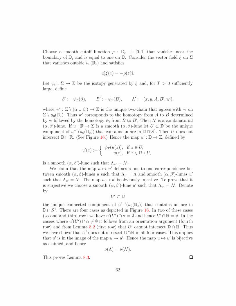
Choose a smooth cutoff function ρ : Dε → [0, 1] that vanishes near theboundary of Dε and is equal to one on D. Consider the vector field ξ on Σthat vanishes outside u0(Dε) and satisfies
u∗0ξ(z) = −ρ(z)i.
Let ψt : Σ → Σ be the isotopy generated by ξ and, for T > 0 sufficientlylarge, define
β ′ := ψT (β), B′ := ψT (B), Λ′ := (x, y, A,B′,w′),
where w′ : Σ \ (α ∪ β ′) → Z is the unique two-chain that agrees with w onΣ \ u0(Dε). Thus w′ corresponds to the homotopy from A to B determinedby w followed by the homotopy ψt from B to B′. Then Λ′ is a combinatorial(α, β ′)-lune. If u : D → Σ is a smooth (α, β)-lune let U ⊂ D be the uniquecomponent of u−1(u0(Dε)) that contains an arc in D ∩ S1. Then U does notintersect D ∩ R. (See Figure 16.) Hence the map u′ : D → Σ, defined by
u′(z) :=
ψT (u(z)), if z ∈ U,
u(z), if z ∈ D \ U,
is a smooth (α, β ′)-lune such that Λu′ = Λ′.We claim that the map u 7→ u′ defines a one-to-one correspondence be-
tween smooth (α, β)-lunes u such that Λu = Λ and smooth (α, β ′)-lunes u′
such that Λu′ = Λ′. The map u 7→ u′ is obviously injective. To prove that itis surjective we choose a smooth (α, β ′)-lune u′ such that Λu′ = Λ′. Denoteby
U ′ ⊂ D
the unique connected component of u′−1(u0(Dε)) that contains an arc inD ∩ S1. There are four cases as depicted in Figure 16. In two of these cases(second and third row) we have u′(U ′)∩α = ∅ and hence U ′ ∩R = ∅. In thecasees where u′(U ′) ∩ α 6= ∅ it follows from an orientation argument (fourthrow) and from Lemma 8.2 (first row) that U ′ cannot intersect D ∩ R. Thuswe have shown that U ′ does not intersect D∩R in all four cases. This impliesthat u′ is in the image of the map u 7→ u′. Hence the map u 7→ u′ is bijectiveas claimed, and hence
ν(Λ) = ν(Λ′).
This proves Lemma 8.3.
62

Proof of Theorems 6.7 and 6.8. Assume first that Σ is simply connected. Weprove that (iii) implies (i) in Theorem 6.7. Let Λ be a combinatorial (α, β)-lune. By Lemma 8.3, reduce the number of intersection points of Λ, whileleaving the number ν(Λ) unchanged. Continue by induction until reaching anembedded combinatorial lune in Σ. By Proposition 7.4, such a lune satisfiesν = 1. Hence ν(Λ) = 1. In other words, there is a smooth (α, β)-luneu : D → Σ, unique up to equivalence, such that Λu = Λ. Thus we haveproved that (iii) implies (i). We have also proved, in the simply connectedcase, that u is uniquely determined by Λu up to equivalence. From now onwe drop the hypothesis that Σ is simply connected.
We prove Theorem 6.8. Let u : D → Σ and u′ : D → Σ be smooth(α, β)-lunes such that
Λu = Λu′.
Let u : D → Σ and u′ : D → Σ be lifts to the universal cover such that
u(−1) = u′(−1).
Then Λeu = Λeu′. Hence, by what we have already proved, u is equivalent tou′ and hence u is equivalent to u′. This proves Theorem 6.8.
We prove that (i) implies (ii) in Theorem 6.7. Let u : D → Σ be a smooth(α, β)-lune and denote by Λu =: (x, y, A,B,w) be its (α, β)-trace. Thenw(z) = #u−1(z) is the counting function of u and hence is nonnegative. For0 < t ≤ 1 define the curve λt : [0, 1] → RP1 by
du(− cos(πs), t sin(πs))λt(s) := R∂
∂su(− cos(πs), t sin(πs)), 0 ≤ s ≤ 1.
For t = 0 use the same definition for 0 < s < 1 and extend the curvecontinuously to the closed interval 0 ≤ s ≤ 1. Then
λ0(s) = du(− cos(πs), 0)−1Tu(− cos(πs),0)α,
λ1(s) = du(− cos(πs), sin(πs))−1Tu(− cos(πs),sin(πs))β,0 ≤ s ≤ 1.
The Viterbo–Maslov index µ(Λu) is, by definition, the relative Maslov indexof the pair of Lagrangian paths (λ0, λ1), denoted by µ(λ0, λ1) (see Defini-tion 3.1 above or [39, 30]). Hence it follows from the homotopy axiom forthe relative Maslov index that
µ(Λu) = µ(λ0, λ1) = µ(λ0, λt)
for every t > 0. Choosing t sufficiently close to zero we find that µ(Λu) = 1.
63

We prove that (iii) implies (ii) in Theorem 6.7. If Λ = (x, y,w) is acombinatorial (α, β)-lune, then w ≥ 0 by (I) in Definition 6.6. Moreover, bythe trace formula (37), we have
µ(Λ) =mx(Λ) +my(Λ)
2.
It follows from (II) and (III) in Definition 6.6 that mx(Λ) = my(Λ) = 1 andhence µ(Λ) = 1. Thus we have proved that (iii) implies (ii).
We prove that (ii) implies (iii) in Theorem 6.7. Let Λ = (x, y,w) bean (α, β)-trace such that w ≥ 0 and µ(Λ) = 1. Denote να := ∂w|α\β andνβ := −∂w|β\α. Reversing the orientation of α or β, if necessary, we mayassume that να ≥ 0 and νβ ≥ 0. Let εx, εy ∈ ±1 be the intersection indicesof α and β at x, y with these orientations, and let
nα := min να ≥ 0, nβ := min νβ ≥ 0.
As before, denote by mx (respectively my) the sum of the four values of wencountered when walking along a small circle surrounding x (respectvely y).Since the Viterbo–Maslov index of Λ is odd, we have εx 6= εy and thus x 6= y.This shows that Λ satisfies the arc condition if and only if nα = nβ = 0.
We prove that Λ satisfies (II). Suppose, by contradiction, that Λ does notsatisfy (II). Then εx = −1 and εy = 1. This implies that the values of wnear x are given by k, k + nα + 1, k + nα + nβ + 1, k + nβ + 1 for someinteger k. Since w ≥ 0 these numbers are all nonnegative. Hence k ≥ 0 andhence mx ≥ 3. The same argument shows that my ≥ 3 and, by the traceformula (37), we have µ(Λ) = (mx(Λ) +my(Λ))/2 ≥ 3, in contradiction toour hypothesis. This shows that Λ satisfies (II).
We prove that Λ satisfies the arc condition and (III). By (II) we haveεx = 1. Hence the values of w near x in counterclockwise order are given bykx, kx + nα + 1, kx + nα − nβ, kx − nβ for some integer kx ≥ nβ ≥ 0. Thisimplies
mx(Λ) = 4kx − 2nβ + 2nα + 1
and, similarly, my(Λ) = 4ky − 2nβ + 2nα + 1 for some integer ky ≥ nβ ≥ 0.Hence, by the trace formula (37), we have
1 = µ(Λ) =mx(Λ) +my(Λ)
2= kx + (kx − nβ) + ky + (ky − nβ) + 2nα + 1.
Hence kx = ky = nα = nβ = 0 and so Λ satisfies the arc condition and (III).Thus we have shown that (ii) implies (i). This proves Theorem 6.7.
64

Example 8.4. The arguments in the proof of Theorem 6.7 can be used toshow that, if Λ is an (α, β)-trace with µ(Λ) = 1, then (I) =⇒ (III) =⇒ (II).Figure 17 shows three (α, β)-traces that satisfy the arc condition and haveViterbo–Maslov index one but do not satisfy (I); one that still satisfies (II)and (III), one that satisfies (II) but not (III), and one that satisfies neither (II)nor (III). Figure 18 shows an (α, β)-trace of Viterbo–Maslov index two thatsatisfies (I) and (III) but not (II). Figure 19 shows an (α, β)-trace of Viterbo–Maslov index three that satisfies (I) and (II) but not (III).
−1−1
11
1
−1
12
Figure 17: Three (α, β)-traces with Viterbo–Maslov index one.
1
Figure 18: An (α, β)-trace with Viterbo–Maslov index two.
1
2
Figure 19: An (α, β)-trace with Viterbo–Maslov index three.
We close this section with two results about lunes that will be usefulbelow.
65

Proposition 8.5. Assume (H) and suppose that α and β are noncontractiblenonisotopic transverse embedded circles and let x, y ∈ α ∩ β. Then there isat most one (α, β)-trace from x to y that satisfies the arc condition. Hence,by Theorems 6.5 and 6.8, there is at most one equivalence class of smooth(α, β)-lunes from x to y.
Proof. Letα = α1 ∪ α2, β = β1 ∪ β2,
where α1 and α2 are the two arcs of α with endpoints x and y, and similarlyfor β. Assume that the quadruple (x, y, α1, β1) is an (α, β)-trace. Then α1 ishomotopic to β1 with fixed endpoints. Since α is not contractible, α2 is nothomotopic to β1 with fixed endpoints. Since β is not contractible, β2 is nothomotopic to α1 with fixed endpoints. Since α is not isotopic to β, α2 is nothomotopic to β2 with fixed endpoints. Hence the quadruple (x, y, αi, βj) isnot an (α, β)-trace unless i = j = 1. This proves Proposition 8.5.
The hypotheses that the loops α and β are not contractible and notisotopic to each other cannot be removed in Proposition 8.5. A pair of isotopiccircles with precisely two intersection points is an example. Another exampleis a pair consisting of a contractible and a non-contractible loop, again withprecisely two intersection points.
Proposition 8.6. Assume (H). If there is a smooth (α, β)-lune then thereis a primitive (α, β)-lune.
Proof. The proof has three steps.
Step 1. If α or β is a contractible embedded circle and α∩ β 6= ∅ then thereexists a primitive (α, β)-lune.
Assume α is a contractible embedded circle. Then, by a theorem of Ep-stein [9], there exists an embedded closed disc D ⊂ Σ with boundary ∂D = α.Since α and β intersect transversally, the set D ∩ β is a finite union of arcs.Let A be the set of all arcs A ⊂ α which connect the endpoints of an arcB ⊂ D ∩ β. Then A is a nonempty finite set, partially ordered by inclusion.Let A0 ⊂ α be a minimal element of A and B0 ⊂ D ∩ β be the arc withthe same endpoints as A0. Then A0 and B0 bound a primitive (α, β)-lune.This proves Step 1 when α is a contractible embedded circle. When β is acontractible embedded circle the proof is analogous.
66

Step 2. Assume α and β are not contractible embedded circles. If thereexists a smooth (α, β)-lune then there exists an embedded (α, β)-lune u suchthat u−1(α) = D ∩ R.
Let v : D → Σ be a smooth (α, β)-lune. Then the set
X := v−1(α) ⊂ D
is a smooth 1-manifold with boundary ∂X = v−1(α)∩S1. The interval D∩R
is one component of X and no component of X is a circle. (If X0 ⊂ X isa circle, then v|X0 : X0 → Σ is a contractible loop covering α finitely manytimes. Hence, by Lemma A.3 in the appendix, it would follow that α is acontractible embedded circle, in contradiction to the hypothesis of Step 2.)Write
∂X = eiθ1, . . . , eiθn, π = θ1 > θ2 > · · · > θn−1 > θn = 0.
Then there is a permutation σ ∈ Sn such that the arc of v−1(α) that startsat eiθj ends at eiθσ(j). This permutation satisfies σ σ = id, σ(1) = n, and
j < k < σ(j) =⇒ j < σ(k) < σ(j).
Hence, by induction, there exists a j ∈ 1, . . . , n−1 such that σ(j) = j+1.Let X0 ⊂ X be the submanifold with boundary points eiθj and eiθj+1 anddenote
Y0 :=eiθ | θj+1 ≤ θ ≤ θj
.
Then the closure of the domain ∆ ⊂ D bounded byX0 and Y0 is diffeomorphicto the half disc and ∆ ∩ v−1(α) = X0. Hence there exists an orientationpreserving embedding ϕ : D → D that maps D∩R onto X0 and maps D∩S1
onto Y0. It follows thatu := v ϕ : D → Σ
is a smooth (α, β)-lune such that
u−1(α) = ϕ−1(∆ ∩ v−1(α)) = ϕ−1(X0) = D ∩ R.
Moreover, Λu = (x, y, A,B,w) with
x := v(eiθj), y := v(eiθj+1), A := v(X0), B := v(Y0).
Since A ∩ B = α ∩ B = x, y, it follows from Proposition 7.4 that u is anembedding. This proves Step 2.
67

Step 3. Assume α and β are not contractible embedded circles. If thereexists an embedded (α, β)-lune u such that u−1(α) = D ∩ R then there existsa primitive (α, β)-lune.
Repeat the argument in the proof of Step 2 with v replaced by u and the setv−1(α) replaced by the 1-manifold
Y := u−1(β) ⊂ D
with boundary∂Y = u−1(β) ∩ R.
The argument produces an arc Y0 ⊂ Y with boundary points a < b such thatthe closed interval X0 := [a, b] intersects Y only in the endpoints. Hence thearcs A0 := u(X0) and B0 := u(Y0) bound a primitive (α, β)-lune. This provesStep 3 and Proposition 8.6.
68

III. Floer Homology
9 Combinatorial Floer Homology
We assume throughout this section that Σ is an oriented 2-manifold withoutboundary and that α, β ⊂ Σ are noncontractible nonisotopic transverse em-bedded circles. We orient α and β. There are three ways we can count thenumber of points in their intersection:
• The numerical intersection number num (α, β) is the actual num-ber of intersection points.
• The geometric intersection number geo (α, β) is defined as the min-imum of the numbers num (α, β ′) over all embedded loops β ′ that aretransverse to α and isotopic to β.
• The algebraic intersection number alg (α, β) is the sum
α · β =∑
x∈α∩β
±1
where the plus sign is chosen iff the orientations match in the directsum TxΣ = Txα⊕ Txβ.
Note that |alg (α, β)| ≤ geo (α, β) ≤ num (α, β).
Theorem 9.1. Define a chain complex ∂ : CF(α, β) → CF(α, β) by
CF(α, β) =⊕
x∈α∩β
Z2x, ∂x =∑
y
n(x, y)y, (45)
where n(x, y) denotes the number modulo two of equivalence classes of smooth(α, β)-lunes from x to y. Then
∂ ∂ = 0.
The homology group of this chain complex is denoted by
HF(α, β) := ker ∂/im∂
and is called the Combinatorial Floer Homology of the pair (α, β).
Proof. See Section 10 page 81.
69

Theorem 9.2. Combinatorial Floer homology is invariant under isotopy:If α′, β ′ ⊂ Σ are noncontractible transverse embedded circles such that α isisotopic to α′ and β is isotopic to β ′ then
HF(α, β) ∼= HF(α′, β ′).
Proof. See Section 11 page 84.
Theorem 9.3. Combinatorial Floer homology is isomorphic to the originalanalytic Floer homology. In fact, the two chain complexes agree.
Proof. See Section 12 page 100.
Corollary 9.4. If geo (α, β) = num (α, β) there is no smooth (α, β)-lune.
Proof. If there exists a smooth (α, β)-lune then, by Proposition 8.6, thereexists a primitive (α, β)-lune and hence there exists an embedded curve β ′
that is isotopic to β and satisfies num (α, β ′) < num (α, β). This contradictsour hypothesis.
Corollary 9.5. dimHF(α, β) = geo (α, β).
Proof. By Theorem 9.2 we may assume that num (α, β) = geo (α, β). Inthis case there is no (α, β)-lune by Corollary 9.4. Hence the Floer boundaryoperator is zero, and hence the dimension of
HF(α, β) ∼= CF(α, β)
is the geometric intersection number geo (α, β).
Corollary 9.6. If geo (α, β) < num (α, β) there is a primitive (α, β)-lune.
Proof. By Corollary 9.5, the Floer homology group has dimension
dim HF(α, β) = geo (α, β).
Since the Floer chain complex has dimension
dim CF(α, β) = num (α, β)
it follows that the Floer boundary operator is nonzero. Hence there existsa smooth (α, β)-lune and hence, by Proposition 8.6, there exists a primitive(α, β)-lune.
70

Remark 9.7 (Action Filtration). Consider the space
Ωα,β := x ∈ C∞([0, 1],Σ) | x(0) ∈ α, x(1) ∈ β
of paths connecting α to β. Every intersection point x ∈ α ∩ β determinesa constant path in Ωα,β and hence a component of Ωα,β . In general, Ωα,β isnot connected and different intersection points may determine different com-ponents (see [29] for the case Σ = T2). By Proposition A.1 in Appendix A,each component of Ωα,β is simply connected. Now fix a positive area form ωon Σ and define a 1-form Θ on Ωα,β by
Θ(x; ξ) :=
∫ 1
0
ω(x(t), ξ(t)) dt
for x ∈ Ωα,β and ξ ∈ TxΩα,β . This form is closed and hence exact. Let
A : Ωα,β → R
be a function whose differential is Θ. Then the critical points of A are thezeros of Θ. These are the constant paths and hence the intersection pointsof α and β. If x, y ∈ α ∩ β belong to the same connected component of Ωα,β
then
A(x)−A(y) =
∫u∗ω
where u : [0, 1]× [0, 1] → Σ is any smooth function that satisfies
u(0, t) = x(t), u(0, 1) = y(t), u(s, 0) ∈ α, u(s, 1) ∈ β
for all s and t (i.e. the map s 7→ u(s, ·) is a path in Ωα,β connecting x to y).In particular, if x and y are the endpoints of a smooth lune then A(x)−A(y)is the area of that lune. Figure 20 shows that there is no upper bound(independent of α and β in fixed isotopy classes) on the area of a lune.
Proposition 9.8. Define a relation ≺ on α∩β by x ≺ y if and only if thereis a sequence x = x0, x1, . . . , xn = y in α ∩ β such that, for each i, there is alune from xi to xi−1 (see Figure 21). Then ≺ is a strict partial order.
Proof. Since there is an (α, β)-lune from xi to xi−1 we have A(xi−1) < A(xi)for every i and hence, by induction, A(x0) < A(xk).
71

Figure 20: A lune of large area.
x x x x x5 3 2 1 0
x4
Figure 21: Lunes from xi to xi−1.
72

Remark 9.9 (Mod Two Grading). The endpoints of a lune have oppositeintersection indices. Thus we may choose a Z/2Z-grading of CF(α, β) by firstchoosing orientations of α and β and then defining CF0(α, β) to be generatedby the intersection points with intersection index +1 and CF1(α, β) to begenerated by the intersection points with intersection index −1. Then theboundary operator interchanges these two subspaces and we have
alg (α, β) = dimHF0(α, β)− dimHF1(α, β).
Remark 9.10 (Integer Grading). Since each component of the path spaceΩα,β is simply connected the Z/2Z-grading in Remark 9.9 can be refined toan integer grading. The grading is only well defined up to a global shift andthe relative grading is given by the Viterbo–Maslov index. Then we obtain
alg (α, β) = χ(HF(α, β)) =∑
i∈Z
(−1)i dimHFi(α, β).
Figure 21 shows that there is no upper or lower bound on the relative indexin the combinatorial Floer chain complex. Figure 22 shows that there is noupper bound on the dimension of CFi(α, β).
In the case of the 2-torus Σ = T2 = R2/Z2 the shift in the integer gradingcan be fixed using Seidel’s notion of a graded Lagrangian submanifold [33].Namely, the tangent bundle of T2 is trivial so that each tangent space isequipped with a canonical isomorphism to R2. Hence every embedded circleα ⊂ T2 determines a map α → RP1 : z 7→ Tzα. A grading of α is a lift ofthis map to the universal cover of RP1. A choice of gradings for α and β canbe used to fix an integer grading of the combinatorial Floer homology.
x y1
y y y y5432
Figure 22: Lunes from x to yi.
73

Remark 9.11 (Integer Coefficients). One can define combinatorial Floerhomology with integer coefficients as follows. Fix an orientation of α. Theneach (α, β)-lune u : D → Σ comes with a sign
ν(u) :=
+1, if the arc u|D∩R : D ∩ R → α is orientation preserving,−1, if the arc u|D∩R : D ∩ R → α is orientation reversing.
Now define the chain complex by
CF(α, β;Z) =⊕
x∈α∩β
Zx,
and∂x :=
∑
y∈α∩β
n(x, y;Z)y, n(x, y;Z) :=∑
[u]
ν(u),
where the sum runs over all equivalence classes [u] of smooth (α, β)-lunesfrom x to y. The results of Section 10 show that Theorem 9.1 remains validwith this refinement, and the results of Section 11 show that Theorem 9.2 alsoremains valid. We will not discuss here any orientation issue for the analyticFloer theory and leave it to others to investigate the validity of Theorem 9.3with integer coefficients.
10 Hearts
Definition 10.1. Let x, z ∈ α ∩ β. A broken (α, β)-heart from x to z isa triple
h = (u, y, v)
such that y ∈ α∩β, u is a smooth (α, β)-lune from x to y, and v is a smooth(α, β)-lune from y to z. The point y is called the midpoint of the heart.By Theorem 6.8 the broken (α, β)-heart h is uniquely determined by the
septuple
Λh := (x, y, z, u(D ∩ R), v(D ∩ R), u(D ∩ S1), v(D ∩ S1)).
Two broken (α, β)-hearts h = (u, y, z) and h′ = (u′, y′, z′) from x to z arecalled equivalent if y′ = y, u′ is equivalent to u, and v′ is equivalentto v. The equivalence class of h is denoted by [h] = ([u], y, [v]). The set ofequivalence classes of broken (α, β)-hearts from x to z will be denoted byH(x, z).
74

Proposition 10.2. Let h = (u, y, v) be a broken (α, β)-heart from x to z andwrite Λh =: (x, y, z, Axy, Ayz, Bxy, Byz). Then exactly one of the following fouralternatives (see Figure 23) holds:
(a) Axy ∩Ayz = y, Byz ( Bxy. (b) Axy ∩Ayz = y, Bxy ( Byz.
(c) Bxy ∩Byz = y, Ayz ( Axy. (d) Bxy ∩Byz = y, Axy ( Ayz.
(a)
(c)
(b)
(d)
x x
yy
zz
x x
z
y
z
y
Figure 23: Four broken hearts.
Proof. The combinatorial (α, β)-lunes Λxy := Λu and Λyz := Λv have bound-aries
∂Λxy = (x, y, Axy, Bxy), ∂Λyz = (y, z, Ayz, Byz)
and their catenation Λxz := Λxy#Λyz = (x, z,wxy+wyz) has Viterbo–Maslovindex two, by (38). Hence mx(Λxy) +mx(Λyz) +mz(Λxy) +mz(Λyz) = 4, bythe trace formula (37). Since mx(Λxy) = mz(Λyz) = 1 this implies
mx(Λyz) +mz(Λxy) = 2. (46)
By Proposition 9.8 we have x 6= z. Hence x cannot be an endpoint of Λyz.Thus mx(Λyz) ≥ 2 whenever x ∈ Ayz ∪ Byz and mx(Λyz) ≥ 4 wheneverx ∈ Ayz ∩Byz. The same holds for mz(Λxy). Hence it follows from (46) thatΛxy and Λyz satisfy precisely one of the following conditions.
(a) x /∈ Ayz ∪Byz, z ∈ Bxy \ Axy. (b) x ∈ Byz \ Ayz, z /∈ Axy ∪Bxy.
(c) x /∈ Ayz ∪Byz, z ∈ Axy \Bxy. (d) x ∈ Ayz \Byz, z /∈ Axy ∪Bxy.
This proves Proposition 10.2.
75

Let N ⊂ C be an embedded convex half disc such that
[0, 1] ∪ i[0, ε) ∪ (1 + i[0, ε)) ⊂ ∂N, N ⊂ [0, 1] + i[0, 1]
for some ε > 0 and define
H := ([0, 1] + i[0, 1]) ∪ (i+N) ∪ (1 + i− iN).
(See Figure 24.) The boundary of H decomposes as
∂H = ∂0H ∪ ∂1H
where ∂0H denotes the boundary arc from 0 to 1 + i that contains the hor-izontal interval [0, 1] and ∂1H denotes the arc from 0 to 1 + i that containsthe vertical interval i[0, 1].
H
δ Η0
δ Η11+i
0
N
Figure 24: The domains N and H .
Definition 10.3. Let x, z ∈ α ∩ β. A smooth (α, β)-heart of type (ac)from x to z is an orientation preserving immersion w : H → Σ that satisfies
w(0) = x, w(1 + i) = z, w(∂0H) ( α, w(∂1H) ( β. (ac)
Two smooth (α, β)-hearts w,w′ : H → Σ are called equivalent iff thereexists an orientation preserving diffeomorphism χ : H → H such that
χ(0) = 0, χ(1 + i) = 1 + i, w′ = w χ.
A smooth (α, β)-heart of type (bd) from x to z is a smooth (β, α)-heartof type (ac) from z to x. Let w be a smooth (α, β)-heart of type (ac) from xto y and h = (u, y, v) be a broken (α, β)-heart from x to y of type (a) or (c).
76

The broken heart h is called compatible with the smooth heart w if thereexist orientation preserving embeddings ϕ : D → H and ψ : D → H suchthat
ϕ(−1) = 0, ψ(1) = 1 + i, (47)
H = ϕ(D) ∪ ψ(D), ϕ(D) ∩ ψ(D) = ϕ(∂D) ∩ ψ(∂D), (48)
u = w ϕ, v = w ψ. (49)
Lemma 10.4. Let h = (u, y, v) be a broken (α, β)-heart of type (a), write
Λh =: (x, y, z, Axy, Ayz, Bxy, Byz),
and define Axz and Bxz by
Axz := Axy ∪ Ayz, Bxy =: Bxz ∪ Byz, Bxz ∩ Byz = z.
Let w be a smooth (α, β)-heart of type (ac) from x to z that is compatiblewith h and let ϕ, ψ : D → H be embeddings that satisfy (47), (48), and (49).Then
ϕ(eiθ1) = 1 + i, (50)
where θ1 ∈ [0, π] is defined by u(eiθ1) = z, and
ϕ(D) ∩ ψ(D) = ψ(D ∩ S1), (51)
w(∂0H) = Axz, w(∂1H) = Bxz. (52)
Proof. By definition of a smooth heart of type (ac), w(∂0H) is arc in αconnecting x to z and w(∂1H) is an arc in β connecting x to z. Moreover,by (49),
ϕ(D ∩ R) ∪ ψ(D ∩ R) ⊂ w−1(α), ϕ(D ∩ S1) ∪ ψ(D ∩ S1) ⊂ w−1(β).
Now w−1(α) is a union of disjoint embedded arcs, and so is w−1(β). One ofthe arcs in w−1(α) contains ∂0H and one of the arcs in w−1(β) contains ∂1H .Since ϕ(−1) = 0 ∈ ∂0H and the arc
w ϕ(D ∩ R) = u(D ∩ R) = Axy
does not contain z we have
ϕ(D ∩ R) ⊂ ∂0H, Axy ⊂ w(∂0H).
77

This implies the first equation in (52). Since wϕ(D∩S1) = u(D∩S1) = Bxy
is an arc containing z we have
∂1H ⊂ ϕ(D ∩ S1), w(∂1H) ⊂ Bxy.
This implies the second equation in (52).We prove (51). Choose θ1 ∈ [0, π] so that u(eiθ1) = z and denote
S0 :=eiθ | 0 ≤ θ ≤ θ1
, S1 :=
eiθ | θ1 ≤ θ ≤ π
,
So that
D ∩ S1 = S0 ∪ S1, u(S0) = Byz, u(S1) = Bxz.
Hence w ϕ(S1) = u(S1) = Bxz = w(∂1H) and 0 ∈ ϕ(S1) ∩ ∂1H . Since w isan immersion it follows that
ϕ(S1) = ∂1H, ϕ(eiθ1) = 1 + i = ψ(1).
This proves (50). Moreover, by (49),
w ϕ(S0) = u(S0) = Byz = v(D ∩ S1) = w ψ(D ∩ S1)
and 1 + i is an endpoint of both arcs ϕ(S0) and ψ(D ∩ S1). Since w is animmersion it follows that
ψ(D ∩ S1) = ϕ(S0) ⊂ ϕ(D) ∩ ψ(D).
To prove the converse inclusion, let ζ ∈ ϕ(D) ∩ ψ(D). Then, by definitionof a smooth heart, ζ ∈ ϕ(∂D) ∩ ψ(∂D). If ζ ∈ ϕ(D ∩ R) ∩ ψ(D ∩ R) thenw(ζ) ∈ Axy ∩ Ayz = y and hence ζ = ψ(−1) ∈ ψ(D ∩ S1). Now supposeζ = ϕ(eiθ) ∈ ψ(D∩R) for some θ ∈ [0, π]. Then we claim that θ ≤ θ1. To seethis, consider the curve ψ(D∩R). By (49), this curve is mapped to Ayz underw and it contains the point ψ(1) = 1+ i. Hence ψ(D∩R) ⊂ ∂0H \ 0. Butif θ > θ1 then ϕ(e
iθ) ∈ ∂1H \1+ i and this set does not intersect ∂0H \0.Thus we have proved that θ ≤ θ1 and hence ϕ(eiθ) ∈ ϕ(S0) = ψ(D ∩ S1), asclaimed. This proves Lemma 10.4.
Proposition 10.5. (i) Let h = (u, y, v) be a broken (α, β)-heart of type (a)or (c) from x to z. Then there exists a smooth (α, β)-heart w of type (ac)from x to z, unique up to equivalence, that is compatible with h.
(ii) Let w be a smooth (α, β)-heart of type (ac) from x to z. Then there existsprecisely one equivalence class of broken (α, β)-hearts of type (a) from x to zthat are compatible with w, and precisely one equivalence class of broken(α, β)-hearts of type (c) from x to z that are compatible with w.
78

Proof. We prove (i). Write
Λh =: (x, y, z, Axy, Ayz, Bxy, Byz)
and assume first that Λh satisfies (a). We prove the existence of [w]. Choosea Riemannian metric on Σ such that the direct sum decompositions
TyΣ = Tyα⊕ Tyβ, TzΣ = Tzα⊕ Tzβ
are orthogonal and α intersects small neighborhoods of y and z in geodesicarcs. Choose a diffeomorphism γ : [0, 1] → Byz such that γ(0) = y andγ(1) = z and let ζ(t) ∈ Tγ(t)Σ be a unit normal vector field pointing to theright. Then there are orientation preserving embeddings ϕ, ψ : D → H suchthat
ϕ(D) = ([0, 1] + i[0, 1]) ∪ (i+N), ϕ(D ∩ R) = [0, 1],
ψ(D) = 1 + i− iN, ψ(D ∩ S1) = 1 + i[0, 1],
andu ϕ−1(1 + s+ it) = expγ(t)(sζ(t))
for 0 ≤ t ≤ 1 and small s ≤ 0, and
v ψ−1(1 + s+ it) = expγ(t)(sζ(t))
for 0 ≤ t ≤ 1 and small s ≥ 0. The function w : H → Σ, defined by
w(z) :=
u ϕ−1(z), if z ∈ ϕ(D),v ψ−1(z), if z ∈ ψ(D),
is a smooth (α, β)-heart of type (ac) from x to z that is compatible with h.We prove the uniqueness of [w]. Suppose that w′ : H → Σ is another
smooth (α, β)-heart of type (ac) that is compatible with h. Let ϕ′ : D → Hand ψ′ : D → H be embeddings that satisfy (47) and (48) and suppose thatw′ is given by (49) with ϕ and ψ replaced by ϕ′ and ψ′. Then
w′ ϕ′ ϕ−1(1 + it) = u ϕ−1(1 + it)
= v ψ−1(1 + it)
= w′ ψ′ ψ−1(1 + it)
for 0 ≤ t ≤ 1 and, by (47) and (50),
ϕ′ ϕ−1(1 + i) = 1 + i = ψ′ ψ−1(1 + i).
79

Since w′ is an immersion it follows that
ϕ′ ϕ−1(1 + it) = ψ′ ψ−1(1 + it) (53)
for 0 ≤ t ≤ 1. Consider the map χ : H → H given by
χ(ζ) :=
ϕ′ ϕ−1(ζ), for ζ ∈ ϕ(D),ψ′ ψ−1(ζ), for ζ ∈ ψ(D).
By (53), this map is well defined. Since H = ϕ′(D) ∪ ψ′(D), the map χ issurjective. We prove that χ is injective. Let ζ, ζ ′ ∈ H such that χ(ζ) = χ(ζ ′).If ζ, ζ ′ ∈ ϕ(D) or ζ, ζ ′ ∈ ψ(D) then it is obvious that ζ = ζ ′. Hence assumeζ ∈ ϕ(D) and ζ ′ ∈ ψ(D). Then ϕ′ ϕ−1(ζ) = ψ′ ψ−1(ζ ′) and hence, by (51),
ψ′ ψ−1(ζ ′) ∈ ψ′(D ∩ S1).
Hence ζ ′ ∈ ψ(D ∩ S1) ⊂ ϕ(D), so ζ and ζ ′ are both contained in ϕ(D),and it follows that ζ = ζ ′. Thus we have proved that χ : H → H is ahomeomorphism. Since w′ = wχ it follows that χ is a diffeomorphism. Thisproves (i) in the case (a). The case (c) follows by reversing the orientationof Σ and replacing u, v, w by
u′ = u ρ, v′ = v ρ, w′(ζ) = w(iζ), ρ(ζ) =i+ ζ
1 + iζ.
Thus ρ : D → D is an orientation reversing diffeomorphism with fixed points±1 that interchanges D ∩ R and D ∩ S1. The map H → H : ζ 7→ iζ isan orientation reversing diffeomorphism with fixed points 0 and 1 + i thatinterchanges ∂0H and ∂1H . This proves (i).
We prove (ii). Let w : H → Σ be a smooth (α, β)-heart of type (ac) anddenote
Axz := w(∂0H), Bxz := w(∂1H).
Let γ ⊂ w−1(β) be the arc that starts at 1+i and points into the interior ofH .Let η ∈ ∂H denote the second endpoint of γ. Since β has no self-intersectionswe have y := w(η) ∈ Axz. The arc γ divides H into two components, eachof which is diffeomorphic to D. (See Figure 25.) The component whichcontains 0 gives rise to a smooth (α, β)-lune u from x to y and the othercomponent gives rise to a smooth (α, β)-lune v from y to z. Let
∂Λu =: (x, y, Axy, Bxy), ∂Λv =: (y, z, Ayz, Byz).
80

−1
−1 −1
H
γ
w (z)
w (x) w (y)
Figure 25: Breaking a heart.
ThenBxy = Bxz ∪Byz, Byz = w(γ).
By Theorem 6.5, Bxy is an arc. Hence Byz ( Bxy, and hence, by Proposi-tion 10.2, the broken (α, β)-heart h = (u, y, v) from x to z satisfies (a). It isobviously compatible with w. A similar argument, using the arc γ′ ⊂ w−1(α)that starts at 1+ i and points into the interior of H , proves the existence of abroken (α, β)-heart h′ ∈ H(x, z) that satisfies (c) and is compatible with w.
If h = (u, y, v) is any other broken (α, β)-heart of type (a) that is compatiblewith w, then it follows from uniqueness in part (i) that w−1(y) = η is the
endpoint of γ, hence y = y, and hence, by Proposition 8.5, h is equivalentto h. This proves (ii) and Proposition 10.5.
Proof of Theorem 9.1. The square of the boundary operator is given by
∂∂x =∑
z∈α∩β
nH(x, z)z,
wherenH(x, z) :=
∑
y∈α∩β
n(x, y)n(y, z) = #H(x, z).
By Proposition 10.5, and the analogous result for smooth (α, β)-hearts oftype (bd), there is an involution τ : H(x, z) → H(x, z) without fixed points.Hence nH(x, z) is even for all x and z and hence ∂ ∂ = 0. This provesTheorem 9.1.
81

11 Invariance under Isotopy
Proposition 11.1. Let x, y, x′, y′ ∈ α∩β be distinct intersection points suchthat
n(x, y) = n(x′, y) = n(x, y′) = 1.
Let u : D → Σ be a smooth (α, β)-lune from x to y and assume that theboundary ∂Λu =: (x, y, A,B) of its (α, β)-trace satisfies
A ∩ β = α ∩ B = x, y.
Then there is no smooth (α, β)-lune from x′ to y′, i.e.
n(x′, y′) = 0.
Moreover, extending the arc from x to y (in either α or β) beyond y, weencounter x′ before y′ (see Figures 26 and 27) and the two arcs A′ ⊂ α andB′ ⊂ β from x′ to y′ that pass through x and y form an (α, β)-trace thatsatisfies the arc condition.
x y x’y’
Figure 26: No lune from x′ to y′.
x x’ yy’
Figure 27: Lunes from x or x′ to y or y′.
Proof. The proof has three steps.
Step 1. There exist (α, β)-traces Λx′y = (x′, y,wx′y), Λyx = (y, x,wyx), andΛxy′ = (x, y′,wxy′) with Viterbo–Maslov indices
µ(Λx′y) = 1, µ(Λyx) = −1, µ(Λxy′) = 1
such thatwx′y ≥ 0, wyx ≤ 0, wx,y′ ≥ 0.
82

By hypothesis, there exist smooth (α, β)-lunes from x′ to y, from x to y, andfrom x to y′. By Theorem 6.7 this implies the existence of combinatorial(α, β)-lunes Λx′y = (x′, y,wx′y), Λxy = (x, y,wxy), and Λxy′ = (x, y′,wxy′). Toprove Step 1, reverse the direction of Λxy to obtain the required (α, β)-traceΛyx = (y, x,wyx) with wyx := −wxy.
Step 2. Let Λx′y, Λyx, Λxy′ be as in Step 1. Then
mx′(Λyx) = my′(Λyx) = 0,
mx(Λx′y) = my(Λxy′) = 0,
my′(Λx′y) = mx′(Λxy′) = 0.
(54)
By hypothesis, the combinatorial (α, β)-lune Λxy = Λu has the boundary∂Λxy = (x, y, A,B) with A ∩ β = α ∩ B = x, y. Hence wyx = −wxy
vanishes near every intersection point of α and β other than x and y. Thisproves the first equation in (54). By (38), the (α, β)-trace Λx′x := Λx′y#Λyx
has Viterbo–Maslov index index zero. Hence, by the trace formula (37),
0 = mx′(Λx′x) +mx(Λx′x)
= mx′(Λx′y) +mx′(Λyx) +mx(Λx′y) +mx(Λyx)
= mx(Λx′y).
Here the last equation follows from the fact thatmx′(Λyx) = 0,mx′(Λx′y) = 1,and mx(Λyx) = −1. The equation my(Λxy′) = 0 is proved by an analogousargument, using the fact that Λyy′ := Λyx#Λxy′ has Viterbo–Maslov indexzero. This proves the second equation in (54). To prove the last equationin (54) we observe that the catenation
Λx′y′ := Λx′y#Λyx#Λxy′ = (x′, y′,wx′y + wyx + wxy′) (55)
has Viterbo–Maslov index one. Hence, by the trace formula (37),
2 = mx′(Λx′y′) +my′(Λx′y′)
= mx′(Λx′y) +mx′(Λyx) +mx′(Λxy′)
+my′(Λx′y) +my′(Λyx) +my′(Λxy′)
= 2 +mx′(Λxy′) +my′(Λx′y).
Here the last equation follows from the first equation in (54) and the factthat mx′(Λx′y) = my′(Λxy′) = 1. Since the numbers mx′(Λxy′) and my′(Λx′y)are nonnegative, this proves the last equation in (54). This proves Step 2.
83

Step 3. We prove the Proposition.
Let Λx′y, Λyx, Λxy′ be as in Step 1 and denote
∂Λx′y =: (x′, y, Ax′y, Bx′y),
∂Λyx =: (y, x, Ayx, Byx),
∂Λxy′ =: (x, y′, Axy′ , Bxy′).
By Step 2 we have
x, y′ /∈ Ax′y ∪ Bx′y, x′, y′ /∈ Ayx ∪ Byx, x′, y /∈ Axy′ ∪Bxy′ . (56)
In particular, the arc in α or β from y to x′ contains neither x nor y′. Henceit is the extension of the arc from x to y and we encounter x′ before y′ asclaimed. It follows also from (56) that the catenation Λx′y′ in (55) satisfiesthe arc condition and has boundary arcs
Ax′y′ := Ax′y ∪Ayx ∪Axy′ , Bx′y′ := Bx′y ∪Byx ∪Bxy′ .
Thus x ∈ Ax′y′ and it follows from Step 2 that
mx(Λx′y′) = mx(Λx′y) +mx(Λyx) +mx(Λxy′) = 0.
This shows that the function wx′y′ is not everywhere nonnegative, and henceΛx′y′ is not a combinatorial (α, β)-lune. By Proposition 8.5 there is no other(α, β)-trace with endpoints x′, y′ that satisfies the arc condition. Hencen(x′, y′) = 0. This proves Proposition 11.1
Proof of Theorem 9.2. By composing with a suitable ambient isotopy assumewithout loss of generality that α = α′. Furthermore assume the isotopyβt0≤t≤1 with β0 = β and β1 = β ′ is generic in the following sense. Thereexists a finite sequence of pairs (ti, zi) ∈ [0, 1]× Σ such that
0 < t1 < t2 < · · · < tm < 1,
α ⋔z βt unless (t, z) = (ti, zi) for some i, and for each i there exists acoordinate chart Ui → R2 : z 7→ (ξ, η) at zi such that
α ∩ Ui = η = 0 , βt ∩ Ui =η = −ξ2 ± (t− ti)
(57)
for t near ti. It is enough to consider two cases.
84

Case 1 is m = 0. In this case there exists an ambient isotopy ϕt such thatϕt(α) = α and ϕt(β) = βt. It follows that the map CF(α, β) → CF(α, β ′)induced by ϕ1 : α ∩ β → α ∩ β ′ is a chain isomorphism that identifies theboundary maps.
In Case 2 we have m = 1, the isotopy is supported near U1, and (57) holdswith the minus sign. Thus there are two intersection points in U1 for t < t1,no intersection points in U1 for t > t1, and all other intersection points of αand βt are independent of t. Denote by x, y ∈ α ∩ β the intersection pointsthat cancel at time t = t1 and choose the ordering such that
n(x, y) = 1. (58)
Then α ∩ β ′ = (α ∩ β) \ x, y. We prove in seven steps that
n′(x′, y′) = n(x′, y′) + n(x′, y)n(x, y′) (59)
for x′, y′ ∈ α ∩ β ′, where n(x′, y′) denotes the number of (α, β)-lunes from x′
to y′ and n′(x′, y′) denotes the number of (α, β ′)-lunes from x′ to y′.
Step 1. If there is no (α, β)-trace from x′ to y′ that satisfies the arc conditionthen (59) holds.
In this case there is no (α, βt)-trace from x′ to y′ that satisfies the arc condi-tion for any t. Hence it follows from Theorem 6.5 that n(x′, y′) = n′(x′, y′) = 0and it follows from Proposition 11.1 that n(x′, y)n(x, y′) = 0. Hence (59)holds in this case.
Standing Assumptions, Part 1. From now on we assume that there isan (α, β)-trace from x′ to y′ that satisfies the arc condition. Then there isan (α, βt)-trace from x′ to y′ that satisfies the arc condition for every t. ByProposition 8.5, this (α, βt)-trace is uniquely determined by x′ and y′. Wedenote it by Λx′y′(t) and its boundary by
∂Λx′y′(t) =: (x′, y′, Ax′y′ , Bx′y′(t)).
Choose a universal covering π : C → Σ so that α = R is a lift of α, themap z 7→ z + 1 is a covering transformation, and π maps the interval [0, 1)bijectively onto α. Let
Λx′y′(t) = (x′, y′,weΛx′y′(t))
be a continuous family of lifts of the (α, βt)-traces to the universal cover
π : C → Σ with boundaries ∂Λx′y′(t) = (x′, y′, Ax′y′, Bx′y′(t)).
85

Step 2. The lift Λx′y′(t) satisfies condition (II) (that the intersection index
of Ax′y′ and Bx′y′(t) at x′ is +1 and at y′ is −1) and condition (III) (that
the winding numbers of Ax′y′ − Bx′y′(t) are zero or one near x′ and y′) eitherfor all values of t or for no value of t.
The intersection indices of Ax′y′ and Bx′y′(t) at x′ and y′, and the winding
numbers of Ax′y′ − Bx′y′(t) near x′ and y′, are obviously independent of t.
Step 3. If one of the arcs Ax′y′(t) and Bx′y′(t) does not pass through U1
then (59) holds.
In this case the winding numbers do not change sign as t varies and hence,by Step 2, ν(Λx′y′(t)) is independent of t. Hence
n(x′, y′) = n′(x′, y′).
To prove equation (59) in this case, we must show that one of the numbersn(x′, y) or n(x, y′) vanishes. Suppose otherwise that
n(x′, y) = n(x, y′) = 1.
Since n(x, y) = 1, by equation (58), it follows from Proposition 11.1 that thetwo arcs from x′ to y′ that pass through U1 form an (α, β)-trace that satisfiesthe arc condition. Hence there are two (α, β)-traces from x′ to y′ that satisfythe arc condition, which is impossible by Proposition 8.5. This contradictionproves Step 3.
k
k+1
kk-1
Case 1
k+2
k+1
kk+1
Case 2
k k
k-1 k-1
k-1 k+1
k
Case 3 Case 4
k-2
k-1 k+1
k+1k-1
Figure 28: The winding numbers of Λx′y′ in U1 for t = 0.
86

Standing Assumptions, Part 2. From now on we assume that Ax′y′ andBx′y′(t) both pass through U1. Denote by x and y the unique lifts of x and y,
respectively, in Ax′y′ ∩ Bx′y′(0).
Under this assumption the winding number of Λx′y′(t) only changes in the
area enclosed by the two arcs in the lift U1 of U1 which contains x and y.There are four cases, depending on the orientations of the two arcs from x′
to y′. (See Figure 28.) The next step deals with three of these cases.
Step 4. Assume that the orientation of α from x′ to y′ does not agree withone of the orientations from x′ to y or from x to y′, or else that this holdsfor β (i.e. that one of the Cases 1,2,3 holds in Figure 28). Then (59) holds.
In Cases 1,2,3 the pattern of winding numbers shows (for any value of k) thatweΛx′y′(t)
is either nonnegative for all values of t or is somewhere negative for
all values of t. Hence, by Step 2, ν(Λx′y′(t)) is independent of t, and hencen(x′, y′) = n′(x′, y′). Moreover, by Proposition 11.1, we have that in thesecases n(x, y′)n(x′, y) = 0. Hence (59) holds in the Cases 1,2,3.
Standing Assumptions, Part 3. From now on we assume that Case 4holds in Figure 28, i.e. that the orientations of α and β from x′ to y′ agreewith the orientations from x′ to y and with the orientations from x to y′.
Step 5. Assume Case 4 and n(x′, y) = n(x, y′) = 1. Then (59) holds.
By Proposition 11.1, we have n(x′, y′) = 0. We must prove that n′(x′, y′) = 1.Let Λx′y and Λxy′ be the (α, β)-traces from x′ to y, respectively from x to y′,
that satisfy the arc condition and denote their lifts by Λx′y and Λxy′. By (55),
weΛx′y′(0)(z) = weΛx′y
(z) + weΛxy′(z) for z ∈ C \ U1. (60)
Thus weΛx′y′(0)≥ 0 in C \ U1. Moreover, by Theorem 6.7, the lifts Λx′y, Λxy′
have winding numbers zero in the regions labelled by k and k−1 in Figure 28,Case 4. Hence, by (60), we have k = 0 and hence
weΛx′y′(t)≥ 0 for t > t1.
Thus we have proved that Λx′y′(t) satisfies (I) for t > t1. Moreover, theViterbo–Maslov index is given by
µ(Λx′y′(t)) = µ(Λx′y) + µ(Λxy′)− µ(Λxy) = 1.
Hence, by Theorem 6.7, Λx′y′(t) is a combinatorial lune for t > t1 and wehave n′(x′, y′) = 1.
87

Step 6. Assume Case 4 and n′(x′, y′) = 1. Then (59) holds.
The winding numbers of Λx′y′(1) are nonnegative and hence we must have
k ≥ 0 in Figure 28, Case 4. If k > 0 then the winding numbers of Λx′y′(0)are also nonnegative and hence, by Step 2, n(x′, y′) = 1. Hence, by (58) andProposition 11.1, one of the numbers n(x′, y) and n(x, y′) must vanish, andhence (59) holds when k > 0.
γγ-
t=1t=0
+γ
Figure 29: A lune splits.
Now assume k = 0. Then n(x′, y′) = 0 and we must prove that
n(x′, y) = n(x, y′) = 1.
To see this, we choose a smooth (α, β ′)-lune
u′ : D → C
from x′ to y′. Since k = 0 this lune has precisely one preimage in the regionin U1 where there winding number is k + 1 = 1 6= 0 for t = 1. Choose anembedded arc
γ : [0, 1] → C
in U1 for t = 1 connecting the two branches of α and β ′ such that γ intersectsα and β ′ only at the endpoints (see Figure 29). Then
γ := u′−1(γ)
88

divides D into two components. Deform the curve β ′ along γ to a curveβ ′′ that intersects α in two points x′′, y′′ ∈ U1. The preimage of β ′′ underu′ contains two arcs γ− and γ+, parallel to γ, in the two components ofD. This results in two half-discs contained in D, and the restriction of u tothese two half discs gives rise to two (α, β ′′)-lunes, one from x′ to y′′ and
one from x′′ to y′ (see Figure 29). Moreover β ′′ descends to an embeddedloop in Σ that is isotopic to β through loops that are transverse to α. Hencen(x′, y) = n(x, y′) = 1, as claimed.
Step 7. Assume Case 4 and n′(x′, y′) = n(x′, y)n(x, y′) = 0. Then (59)holds.
We must prove that n(x′, y′) = 0. By Step 2, conditions (II) and (III) on
Λx′y′(t) are independent of t and so we have that n(x′, y′) = 0 whenever these
conditions are not satisfied. Hence assume that Λx′y′(t) satisfies (II) and (III)for every t. If k > 0 in Figure 28 then condition (I) also holds for every t andhence n(x′, y′) = n′(x′, y′) = 1, a contradiction. If k ≤ 0 in Figure 28 then
Λx′y′(0) does not satisfy (I) and hence n(x′, y′) = 0, as claimed.
Thus we have established (59). Hence, by Lemma C.1, HF(α, β) is isomorphicto HF(α, β ′). This proves Theorem 9.2.
12 Lunes and Holomorphic Strips
We assume throughout that Σ and α, β ⊂ Σ satisfy hypothesis (H). Wealso fix a complex structure J on Σ. A holomorphic (α, β)-strip is aholomorphic map v : S → Σ of finite energy such that
v(R) ⊂ α, v(R+ i) ⊂ β. (61)
It follows [32, Theorem A] that the limits
x = lims→−∞
v(s+ it), y = lims→+∞
v(s+ it) (62)
exist; the convergence is exponential and uniform in t; moreover ∂sv andall its derivatives converge exponentially to zero as s tends to ±∞. Calltwo holomorphic strips equivalent if they differ by a time shift. Everyholomorphic strip v has a Viterbo–Maslov index µ(v), defined as follows.Trivialize the complex line bundle v∗TΣ → S such that the trivialization
89
converges to a frame of TxΣ as s tends to −∞ and to a frame of TyΣ ass tends to +∞ (with convergence uniform in t). Then s 7→ Tv(s,0)α ands 7→ Tv(s,1)β are Lagrangian paths and their relative Maslov index is µ(v)(see [39] and [30]).
At this point it is convenient to introduce the notation
MFloer(x, y; J) :=
v : S → Σ
∣∣∣∣v is a holomorphic (α, β)-stripfrom x to y with µ(v) = 1
time shift
for the moduli space of index one holomorphic strips from x to y up to timeshift. This moduli space depends on the choice of a complex structure J onΣ. We also introduce the notation
Mcomb(x, y) :=
u : D → Σ
∣∣∣∣u is a smooth (α, β)-lunefrom x to y
isotopy
for the moduli space of (equivalence classes of) smooth (α, β)-lunes. Thisspace is independent of the choice of J . We show that there is a bijectionbetween these moduli spaces for every pair x, y ∈ α ∩ β.
Given a smooth (α, β)-lune u : D → Σ, the Riemann mapping theoremgives a unique homeomorphism ϕu : D → D such that the restriction of ϕu
to D \ ±1 is a diffeomorphism and
ϕu(−1) = −1, ϕu(0) = 0, ϕu(1) = 1, ϕ∗uu
∗J = i. (63)
Let g : S → D \ ±1 be the holomorphic diffeomorphism given by
g(s+ it) :=e(s+it)π/2 − 1
e(s+it)π/2 + 1. (64)
Then, for every (α, β)-lune u, the composition v := uϕug is a holomorphic(α, β)-strip.
Theorem 12.1. Assume (H), let x, y ∈ α∩β, and choose a complex structureJ on Σ. Then the map u 7→ u ϕu g induces a bijection
Mcomb(x, y) → MFloer(x, y; J) : [u] 7→ [u ϕu g] (65)
between the corresponding moduli spaces.
Proof. See page 97 below.
90

The proof of Theorem 12.1 relies on the asymptotic analysis of holomor-phic strips in [32] (see Appendx D for a summary) and on an explicit formulafor the Viterbo–Maslov index. For each intersection point x ∈ α ∩ β we de-note by θx ∈ (0, π) the angle from Txα to Txβ with respect to our complexstructure J . Thus
Txβ = (cos(θx) + sin(θx)J) Txα, 0 < θx < π. (66)
Fix a nonconstant holomorphic (α, β)-strip v : S → Σ from x to y. Choose aholomorphic coordinate chart ψy : Uy → C on an open neighborhood Uy ⊂ Σof y such that ψy(y) = 0. By [32, Theorem C] (see also Corollary D.2) thereis a complex number cy and a integer νy(v) ≥ 1 such that
ψy(v(s+ it)) = cye−(νy(v)π−θy)(s+it) +O(e−(νy(v)π−θy+δ)s) (67)
for some δ > 0 and all s > 0 sufficiently close to +∞. The complex num-ber cy belongs to the tangent space T0(ψy(α ∩ Uy)) and the integer νy(v) isindependent of the choice of the coordinate chart.
Now let us interchange α and β as well as x and y, and replace v by the(β, α)-holomorphic strip
s+ it 7→ v(−s+ i(1− t))
from y to x. Choose a holomorphic coordinate chart ψx : Ux → C on anopen neighborhood Ux ⊂ Σ of x such that ψx(x) = 0. Using [32, Theorem C]again we find that there is a complex number cx and an integer νx(v) ≥ 0such that
ψx(v(s+ it)) = cxe(νx(v)π+θx)(s+it) + O(e(νx(v)π+θx+δ)s) (68)
for some δ > 0 and all s < 0 sufficiently close to −∞. As before, the complexnumber cx belongs to the tangent space T0(ψx(α∩Ux)) and the integer νx(v)is independent of the choice of the coordinate chart.
Denote the set of critical points of v by
Cv := z ∈ S | dv(z) = 0 .
It follows from Corollary D.2 (i) that this is a finite set. For z ∈ Cv denoteby νz(v) ∈ N the order to which dv vanishes at z. Thus the first nonzeroterm in the Taylor expansion of v at z (in a local holomorphic coordinatechart on Σ centered at v(z)) has order νz(v) + 1.
91

Theorem 12.2. Assume (H) and choose a complex structure J on Σ. Letx, y ∈ α ∩ β and v : S → Σ be a nonconstant holomorphic (α, β)-strip fromx to y. Then the linearized operator Dv associated to this strip in Floertheory is surjective. Moreover, the Viterbo–Maslov index of v is equal to theFredholm index of Dv and is given by the index formula
µ(v) = νx(v) + νy(v) +∑
z∈Cv∩∂S
νz(v) + 2∑
z∈Cv∩int(S)
νz(v). (69)
The right hand side in equation (69) is positive because all summands arenonnegative and νy(v) ≥ 1.
Proof. See page 97 below.
The surjectivity statement in Theorem 12.2 has been observed by manyauthors. A proof for holomorphic polygons is contained in Seidel’s book [34].
We will need a more general index formula (equation (76) below) whichwe explain next. Choose a Riemannian metric on Σ that is compatible withthe complex structure J . This metric induces a Hermitian structure on thepullback tangent bundle v∗TΣ → S and the Hilbert spacesW 1,2(S, v∗TΣ) andL2(S, v∗TΣ) are understood with respect to this induced structure. TheseHilbert spaces are independent of the choice of the metric on Σ, only theirinner products depend on this choice. The linearized operator
Dv : W1,2BC(S, v
∗TΣ) → L2(S, v∗TΣ)
with
W 1,2BC(S, v
∗TΣ) :=
v ∈ W 1,2(S, v∗TΣ)
∣∣∣∣v(s, 0) ∈ Tv(s,0)α ∀s ∈ R
v(s, 1) ∈ Tv(s,1)β ∀s ∈ R
is given byDvv = ∇sv + J∇tv
for v ∈ W 1,2BC(S, v
∗TΣ), where ∇ denotes the Levi-Civita connection. Herewe use the fact that ∇J = 0 because J is integrable. We remark that, first,this is a Fredholm operator for every smooth map v : S → Σ satisfying (61)and (62) (where the convergence is exponential and uniformly in t, and ∂sv,∇s∂sv, ∇s∂tv converge exponentially to zero as s tends to ±∞). Second, thedefinition of the Viterbo–Maslov index µ(v) extends to this setting and itis equal to the Fredholm index of Dv (see [31]) Third, the operator Dv isindependent of the choice of the Riemannian metric whenever v is an (α, β)-holomorphic strip.
92

Next we choose a unitary trivialization
Φ(s, t) : C → Tv(s,t)Σ
of the pullback tangent bundle such that
Φ(s, 0)R = Tv(s,0)α, Φ(s, 1)R = Tv(s,1)β,
and Φ(s, t) = Ψt(v(s, t)) for |s| sufficiently large. Here Ψt, 0 ≤ t ≤ 1,is a smooth family of unitary trivializations of the tangent bundle over aneighborhood Ux ⊂ Σ of x, respectively Uy ⊂ Σ of y, such that Ψ0(z)R = Tzαfor z ∈ (Ux ∪ Uy) ∩ α and Ψ1(z)R = Tzβ for z ∈ (Ux ∪ Uy) ∩ β. Then
W := Φ−1W 1,2BC(S, v
∗TΣ) =ξ ∈ W 1,2(S,C) | ξ(s, 0), ξ(s, 1) ∈ R ∀s ∈ R
,
H := Φ−1L2(S, v∗TΣ) = L2(S,C).
The operator DS := Φ−1 Dv Φ : W → H has the form
DSξ = ∂sξ + i∂tξ + Sξ (70)
where the function S : S → EndR(C) is given by
S(s, t) := Φ(s, t)−1(∇sΦ(s, t) + J(v(s, t))∇tΦ(s, t)
).
The matrix Φ−1∇sΦ is skew-symmetric and the matrix Φ−1J(v)∇tΦ is sym-metric. Moreover, it follows from our hypotheses on v and the trivializationthat S converges exponentially and Φ−1∇sΦ as well as ∂sS converge expo-nentially to zero as as s tends to ±∞. The limits of S are the symmetricmatrix functions
Sx(t) := lims→−∞
S(s, t) = Ψt(x)−1J(x)∂tΨt(x),
Sy(t) := lims→+∞
S(s, t) = Ψt(y)−1J(y)∂tΨt(y).
(71)
Thus there exist positive constants c and ε such that
|S(s, t)− Sx(t)|+ |∂sS(s, t)| ≤ ceεs,
|S(s, t)− Sy(t)|+ |∂sS(s, t)| ≤ ce−εs (72)
for every s ∈ R. This shows that the operator (70) satisfies the hypothesesof [32, Lemma 3.6]. This lemma asserts the following. Let ξ ∈ W be anonzero function in the kernel of DS:
ξ ∈ W, DSξ = ∂sξ + i∂tξ + Sξ = 0, ξ 6= 0.
93

Then there exist nonzero functions ξx, ξy : [0, 1] → C and positive real num-bers λx, λy, C, δ such that
iξx(t) + Sx(t)ξx(t) = −λxξx(t), ξx(0), ξx(1) ∈ R
iξy(t) + Sy(t)ξy(t) = λyξy(t), ξy(0), ξy(1) ∈ R(73)
and∣∣ξ(s, t)− eλxsξx(t)
∣∣ ≤ Ce(λx+δ)s, s ≤ 0∣∣ξ(s, t)− e−λysξy(t)
∣∣ ≤ Ce−(λy+δ)s, s ≥ 0.(74)
We prove that there exist integers ι(x, ξ) ≥ 0 and ι(y, ξ) ≥ 1 such that
λx = ι(x, ξ)π + θx, λy = ι(y, ξ)π − θy. (75)
Here θx is chosen as above such that
Txβ = exp(θxJ(x))Txα, 0 < θx < π,
and the same for θy. To prove (75), we observe that the function
vx(t) := Ψt(x)ξx(t)
satisfies
J(x)vx(t) = −λxvx(t), vx(0) ∈ Txα, vx(1) ∈ Txβ.
Hence vx(t) = exp(tλxJ(x))vx(0) and this proves the first equation in (75).Likewise, the function vy(t) := Ψt(y)ξy(t) satisfies J(y)vy(t) = λyvy(t) andvy(0) ∈ Tyα and vy(1) ∈ Tyβ. Hence vy(t) = exp(−tλyJ(y))vy(0), and thisproves the second equation in (75).
Lemma 12.3. Suppose S satisfies the asymptotic condition (72) and letξ ∈ W be a smooth function with isolated zeros that satisfies (73), (74),and (75). Then the Fredholm index of DS is given by the linear indexformula
index(DS) = ι(x, ξ) + ι(y, ξ) +∑
z∈∂Sξ(z)=0
ι(z, ξ) + 2∑
z∈int(S)ξ(z)=0
ι(z, ξ). (76)
In the second sum ι(z, ξ) denotes the index of z as a zero of ξ. In the firstsum ι(z, ξ) denotes the degree of the loop [0, π] → RP1 : θ 7→ ξ(z + εeiθ)Rwhen z ∈ R and of the loop [0, π] → RP1 : θ 7→ ξ(z − εeiθ)R when z ∈ R+ i;in both cases ε > 0 is chosen so small that the closed ε-neighborhood of zcontains no other zeros of ξ.
94

Proof. Since ξx and ξy have no zeros, by (73), it follows from equation (74)that the zeros of ξ are confined to a compact subset of S. Moreover the zerosof ξ are isolated and so the right hand side of (76) is a finite sum. Now letξ0 : S → C be the unique solution of the equation
i∂tξ0(s, t) + S(s, t)ξ0(s, t) = 0, ξ0(s, 0) = 1. (77)
Then
ξ0,x(t) := lims→−∞
ξ0(s, t) = Ψt(x)−1Ψ0(x)1,
ξ0,y(t) := lims→+∞
ξ0(s, t) = Ψt(y)−1Ψ0(y)1.
(78)
Thus the Lagrangian path
R → RP1 : s 7→ ΛS(s) := Rξ(s, 1)
is asymptotic to the subspace Ψ1(x)−1Txα as s tends to −∞ and to the
subspace Ψ1(y)−1Tyα as s tends to +∞. These subspaces are both transverse
to R. By the spectral-flow-equals-Maslov-index theorem in [31] the Fredholmindex of DS is equal to the relative Maslov index of the pair (ΛS,R):
index(DS) = µ(ΛS,R). (79)
It follows from (73) and (78) that
ξ0,x(t)
ξx(t)=e−iλxt
ξx(0),
ξ0,y(t)
ξy(t)=
eiλyt
ξy(0). (80)
Now let U =⋃
ξ(z)=0 Uz ⊂ S be a union of open discs or half discs Uz of radiusless than one half, centered at the zeros z of ξ, whose closures are disjoint.Consider the smooth map Λ : S \ U → RP1 defined by
Λ(s, t) := ξ0(s, t)ξ(s, t)R.
By (80) this map converges, uniformly in t, as s tends to ±∞ with limits
Λx(t) := lims→−∞
Λ(s, t) = e−iλxtR, Λy(t) := lims→+∞
Λ(s, t) = eiλytR. (81)
Moreover, we have
Λ(s, 1) = ξ0(s, 1)R = ΛS(s), (s, 1) /∈ U,
Λ(s, 0) = ξ0(s, 0)R = R, (s, 0) /∈ U.
95

If z ∈ int(S) with ξ(z) = 0 then the map Λz := Λ|∂Uzis homotopic to the
map ∂Uz → RP1 : s + it 7→ ξ(s, t)R. Hence it follows from the definition ofthe index ι(z, ξ) that its degree is
deg(Λz : ∂Uz → RP1) = −2ι(z, ξ), z ∈ int(S), ξ(z) = 0. (82)
If z ∈ ∂S with ξ(z) = 0, define the map Λz : ∂Uz → RP 1 by
Λz(s, t) :=
ξ0(s, t)ξ(s, t)R, if (s, t) ∈ ∂Uz \ ∂S,ξ0(s, t)R, if (s, t) ∈ ∂Uz ∩ ∂S.
This map is homotopic to the map (s, t) 7→ ξ(s, t)R for (s, t) ∈ ∂Uz \ ∂S and(s, t) 7→ R for (s, t) ∈ ∂Uz ∩ ∂S. Hence it follows from the definition of theindex ι(z, ξ) that its degree is
deg(Λz : ∂Uz → RP1) = −ι(z, ξ), z ∈ ∂S, ξ(z) = 0. (83)
Abbreviate ST := [−T, T ] + i[0, 1] for T > 0 sufficiently large. Since the mapΛ : ∂(ST \U) → RP1 extends to ST \U its degree is zero and it is equal to therelative Maslov index of the pair of Lagrangian loops (Λ|∂(ST∩U),R). Hence
0 = limT→∞
µ(Λ|∂(ST \U),R)
= µ(Λy,R)− µ(Λx,R)− µ(ΛS,R)−∑
z∈S
ξ(z)=0
µ(Λz,R)
= ι(y, ξ) + ι(x, ξ)− µ(ΛS,R) +∑
z∈∂Sξ(z)=0
ι(z, ξ) + 2∑
z∈int(S)ξ(z)=0
ι(z, ξ).
Here the second equality follows from the additivity of the relative Maslovindex for paths [30]. It also uses the fact that, for z ∈ R+ i with ξ(z) = 0, therelative Maslov index of the pair (Λz|∂Uz∩(R+i),R) = (ΛS|∂Uz∩(R+i),R) appearswith a plus sign when using the orientation of R+ i and thus compensates forthe intervals in the relative Maslov index −µ(ΛS,R) that are not containedin the boundary of S \ U . Moreover, for z ∈ R with ξ(z) = 0, the relativeMaslov index of the pair (Λz|∂Uz∩R,R) is zero. The last equation follows fromthe formulas (75) and (81) for the first two terms and from (83) and (82)for the last two terms. With this understood, the linear index formula (76)follows from equation (79). This proves Lemma 12.3.
96

Lemma 12.4. The operator DS is injective whenever index(DS) ≤ 0 and issurjective whenever index(DS) ≥ 0.
Proof. If ξ ∈ W is a nonzero element in the kernel of DS then ξ satisfies thehypotheses of Lemma 12.3. Moreover, every zero of ξ has positive index bythe argument in the proof of Theorem C.1.10 in [20, pages 561/562]. Hencethe index of DS is positive by the linear index formula in Lemma 12.3. Thisshows that DS is injective whenever index(DS) ≤ 0. If DS has nonnegativeindex then the formal adjoint operator η 7→ −∂sη+i∂tη+S
Tη has nonpositiveindex and is therefore injective by what we just proved. Since its kernel is theL2-orthogonal complement of the image ofDS it follows thatDS is surjective.This proves Lemma 12.4.
Proof of Theorem 12.2. The index formula (69) follows from the linear indexformula (76) in Lemma 12.3 with ξ := Φ−1∂sv. The index formula showsthat Dv has positive index for every nonconstant (α, β)-holomorphic stripv : S → Σ. Hence Dv is onto by Lemma 12.4. This proves Theorem 12.2.
Proof of Theorem 12.1. The proof has four steps.
Step 1. The map (65) is well defined.
Let u, u′ : D → Σ be equivalent smooth (α, β)-lunes from x to y. Then thereis an orientation preserving diffeomorphism ϕ : D → D such that ϕ(±1) = ±1and u′ := u ϕ. Consider the holomorphic strips v := u ϕu g : S → Σ and
v′ := u′ ϕu′ g
= u ϕ ϕuϕ g
= v g−1 ϕ−1u ϕ ϕuϕ g.
By the definition of ϕu we have (u ϕu)∗J = i and (u ϕ ϕuϕ)
∗J = i. (Seeequation (63).) Hence the composition ϕ−1
u ϕ ϕuϕ : D \ ±1 → D \ ±1is holomorphic and so is the composition g−1 ϕ−1
u ϕ ϕuϕ g : S → S.Hence this composition is given by a time shift and this proves Step 1.
Step 2. The map (65) is injective.
Let u, u′ : D → Σ be smooth (α, β)-lunes from x to y and define v := uϕugand v′ := u′ ϕu′ g. (See equations (63) and (64).) Assume that v′ = v τfor a translation τ : S → S. Then u′ = u ϕ, where ϕ : D → D is givenby ϕ|D\±1 = ϕu g τ g−1 ϕ−1
u′ and ϕ(±1) = ±1. Since u and u′ areimmersions, it follows that ϕ is a diffeomorphism of D. This proves Step 2.
97

Step 3. Every holomorphic (α, β)-strip v : S → Σ from x to y with Viterbo–Maslov index one is an immersion and satisfies νx(v) = 0 and νy(v) = 1.
This follows immediately from the index formula (69) in Theorem 12.2.
Step 4. The map (65) is surjective.
Let v : S → Σ be a holomorphic (α, β)-strip from x to y with Viterbo–Maslovindex one. By Step 3, v is an immersion and satisfies νx(v) = 0 and νy(v) = 1.Hence it follows from (67) and (68) that
ψy(v(s+ it)) = cye−(π−θy)(s+it) +O(e−(π−θy+δ)s), s > T,
ψx(v(s+ it)) = cxeθx(s+it) +O(e(θx+δ)s), s < −T,
(84)
for T sufficiently large. This implies that the composition
u′ := v g−1 : D \ ±1 → Σ
(g as in equation (64)) is an immersion and extends continuously to D byu′(−1) := x and u′(1) := y. Moreover, locally near z = −1, the image of u′
covers only one of the four quadrants into which Σ is divided by α and β andthe same holds near z = 1.
We must prove that there exists a homeomorphism ϕ : D → D such that
(a) ϕ(±1) = ±1 and ϕ(0) = 0,
(b) ϕ restricts to an orientation preserving diffeomorphism of D \ ±1,
(c) the map u := u′ ϕ−1 : D → Σ is a smooth lune.
Once ϕ has been found it follows from (c) that uϕ = vg−1 : D\±1 → Σis holomorphic and hence ϕ∗u∗J = i. Hence it follows from (a) and (b)that ϕ = ϕu (see equation (63)) and this implies that the equivalence class[v] ∈ MFloer(x, y; J) belongs to the image of our map (65) as claimed.
To construct ϕ, choose a smooth function λ : R → (1/2,∞) such that
λ(s) =
π/2θx, for s ≤ −2,1, for s ≥ −1,
, λ(s) + λ′(s)s > 0. (85)
(For example define λ(s) := π/θx − 1 + (π/θx − 2) /s for −2 ≤ s ≤ −1 toobtain a piecewise smooth function and approximate by a smooth function.)Then the map s 7→ λ(s)s is a diffeomorphism of R. Consider the sets
Kλ :=
es+it
∣∣∣∣ 0 ≤ t ≤π
2λ(s)
, K :=
es+it
∣∣∣∣ 0 ≤ t ≤π
2
.
98

Denote their closures by Kλ := Kλ ∪ 0 and K := K ∪ 0 and define thehomeomorphism ρλ : Kλ → K by ρλ(0) := 0 and
ρλ(es+it) := e(s+it)λ(s), es+it ∈ Kλ.
It restricts to a diffeomorphism from Kλ to K and it satisfies ρλ(ζ) = ζπ/2θx
for |ζ | ≤ e−2 and ρλ(ζ) = ζ for |ζ | ≥ e−1. Consider the map
wλ : Kλ → Σ, wλ(ζ) := u′(ρλ(ζ)− 1
ρλ(ζ) + 1
). (86)
We claim that wλ : Kλ → Σ is a C1 immersion. If ζ := es+it ∈ Kλ with|ζ | = es ≤ e−2 then by (64)
ρλ(es+it)− 1
ρλ(es+it) + 1=e(s+it)π/2θx − 1
e(s+it)π/2θx + 1= g
(θ−1x (s+ it)
).
Insert this as an argument in u′ and use the formula u′ g = v to obtain
wλ(es+it) = u′
(ρλ(e
s+it)− 1
ρλ(es+it) + 1
)= v
(θ−1x (s+ it)
), s ≤ −2. (87)
Thus
ψx (wλ(ζ)) = ψx
(v(θ−1x (s+ it)
))
= cxes+it +O
(e1+δ/θx)s
)
= cxζ +O(|ζ |1+δ/θx
)
for ζ = es+it ∈ Kλ sufficiently small. (Here the second equation followsfrom (84).) Hence the map wλ : Kλ → Σ in (86) is complex differentiableat the origin and d(ψx wλ)(0) = cx. Next we prove that the derivative ofwλ is continuous. To see this, recall that ψx wλ and ψx v are holomorphicwherever defined and denote their complex derivatives by d(ψx wλ) andd(ψx v). Differentiating equation (87) gives
es+itd(ψx wλ)(es+it) = θ−1
x d(ψx v)(θ−1x (s+ it)
).
By Corollary D.2 (i), e−θx(s+it)d(ψx v)(s + it) converges uniformly to θxcxas s tends to −∞. Hence d(ψx wλ)(ζ) = θ−1
x e−(s+it)d(ψx v)(θ−1x (s + it))
converges to cx = d(ψx wλ)(0) as ζ = es+it ∈ Kλ tends to zero. Hence wλ iscontinuously differentiable near the origin and is a C1 immersion as claimed.
99

Now let σλ : Kλ → D \ 1 be any diffeomorphism that satisfies
σλ(ζ) =ζ − 1
ζ + 1for |ζ | ≥ 1.
Define ϕ′′ : D → D and u′′ : D → Σ by ϕ′′(1) := 1, u′′(1) := y, and
ϕ′′(z) :=ρλ(σ
−1λ (z))− 1
ρλ(σ−1λ (z)) + 1
, u′′(z) := u′ ϕ′′(z) = wλ σ−1λ (z)
for z ∈ D \ 1. Then ϕ′′ = id on z ∈ D |Re z ≥ 0, the map ϕ′′ : D → D
satisfies (a) and (b), and u′′|D\1 is an orientation preserving C1 immersion.A similar construction near y yields an orientation preserving C1 immersionu′′′ = u′ ϕ′′′ : D → Σ where ϕ′′′ : D → D satisfies (a) and (b). Nowapproximate u′′′ in the C1-topology by a smooth lune u = u′ ϕ : D → Σ toobtain the required map ϕ. This proves Step 4 and Theorem 12.1.
Proof of Theorem 9.3. By Theorem 12.2, the linearized operator Dv in Floertheory is surjective for every (α, β)-holomorphic strip v. Hence there is aboundary operator on the Z2 vector space CF(α, β) as defined by Floer [10,11] in terms of the mod two count of (α, β)-holomorphic strips. By Theo-rem 12.1 this boundary operator agrees with the combinatorial one definedin terms of the mod two count of (α, β)-lunes. Hence the combinatorial Floerhomology of the pair (α, β) agrees with the analytic Floer homology definedby Floer. This proves Theorem 9.3.
Remark 12.5 (Hearts and Diamonds). We have seen that the combinato-rial boundary operator ∂ on CF(α, β) agrees with Floer’s boundary operatorby Theorem 12.1. Thus we have two proofs that ∂2 = 0: the combinatorialproof using broken hearts and Floer’s proof using his gluing construction.He showed (in much greater generality) that two (α, β)-holomorphic strips ofindex one (one from x to y and one from y to z) can be glued together to giverise to a 1-parameter family of (α, β)-holomorphic strips (modulo time shift)of index two from x to z. This one parameter family can be continued untilit ends at another pair of (α, β)-holomorphic strips of index one (one fromx to some intersection point y′ and one from y′ to z). These one parameterfamilies are in one-to-one correspondence to (α, β)-hearts from x to z. Thiscan be seen geometrically as follows. Each glued (α, β)-holomorphic stripfrom x to z has a critical point on the β-boundary near y for a broken heartof type (a). The 1-manifold is parametrized by the position of the critical
100

value. There is precisely one (α, β)-holomorphic strip in this moduli spacewithout critical point and an angle between π and 2π at z. The critical valuethen moves onto the α-boundary and tends towards y′ at the other end ofthe moduli space giving a broken heart of type (c) (See Figure 23).
Here is an explicit formula for the gluing construction in the two dimen-sional setting. Let h = (u, y, v) be a broken (α, β)-heart of type (a) or (b)from x to z. (Types (c) and (d) are analogous with α and β interchanged.)Denote the left and right upper quadrants by QL := (−∞, 0) + i(0,∞) andQR := (0,∞) + i(0,∞). Define diffeomorphisms ψL : QL → D \ ∂D andψR : QR → D \ ∂D by
ψL(ζ) :=1 + ζ
1− ζ, ψR(ζ) :=
ζ − 1
ζ + 1.
The extensions of these maps to Mobius transformations of the Riemannsphere are inverses of each other. Define the map w : QL ∪QR → Σ by
w(ζ) :=
u(ψL(ζ)), for ζ ∈ QL,v(ψR(ζ)), for ζ ∈ QR.
The maps u ψL and v ψR send suitable intervals on the imaginary axisstarting at the origin to the same arc on β. Modify u and v so that w extendsto a smooth map on the slit upper half plane H \ i[1,∞), still denoted by w.Here H ⊂ C is the closed upper half plane. Define ϕε : D → H by
ϕε(z) :=2εz
1− z2, z ∈ D, 0 < ε < 1.
This map sends the open set int(D) ∩ QL diffeomorphically onto QL and itsends int(D)∩QR diffeomorphically onto QR. It also sends the interval i[0, 1]diffeomorphically onto i[0, ε]. The composition w ϕε : int(D) → Σ extendsto a smooth map on D denoted by wε : D → Σ. An explicit formula for wε is
wε(z) =
u(
1−z2+2εz1−z2−2εz
), if z ∈ D and Re z ≤ 0,
v(
−1+z2+2εz1+z2+2εz
), if z ∈ D and Re z ≥ 0.
The derivative of this map at every point z 6= i is an orientation preservingisomorphism. Its only critical value is the point
cε := u
(1 + iε
1− iε
)= v
(iε− 1
iε+ 1
)∈ β.
101

Note that cε tends to y = u(1) = v(−1) as ε tends to zero. The compositionof wε with a suitable ε-dependent diffeomorphism S → D \ ±1 gives therequired one-parameter family of glued holomorphic strips.
13 Further Developments
There are many directions in which the theory developed in the presentmemoir can be extended. Some of these directions and related work in theliterature are discussed below.
Floer Homology
If one drops the hypothesis that the loops α and β are not contractible andnot isotopic to each other there are three possibilities. In some cases the Floerhomology groups are still well defined and invariant under (Hamiltonian)isotopy, in other cases invariance under isotopy breaks down, and there areexamples with ∂ ∂ 6= 0, so Floer homology is not even defined. All thesephenomena have their counterparts in combinatorial Floer homology.
A case in point is that of two transverse embedded circles α, β ⊂ C inthe complex plane. In this case the boundary operator
∂ : CF(α, β) → CF(α, β)
of Section 9 still satisfies ∂ ∂ = 0. However, ker ∂ = im ∂ and so the(combinatorial) Floer homology groups vanish. This must be true because(combinatorial) Floer homology is still invariant under isotopy and the loopscan be disjoined by a translation.
A second case is that of two transverse embedded loops in the sphereΣ = S2. Here the Floer homology groups are nonzero when the loops inter-sect and vanish otherwise. An interesting special case is that of two equators.(Following Khanevsky we call an embedded circle α ⊂ S2 an equator whenthe two halves of S2 \ α have the same area.) In this case the combinatorialFloer homology groups do not vanish, but are only invariant under Hamilto-nian isotopy. This is an example of the monotone case for Lagrangian Floertheory (see Oh [21]), and the theory developed by Biran–Cornea applies [5].For an interesting study of diameters (analogues of equators for discs) seeKhanevsky [17].
102

A similar case is that of two noncontractible transverse embedded loops
α, β ⊂ Σ
that are isotopic to each other. Fix an area form on Σ. If β is Hamiltonianisotopic to α then the combinatorial Floer homology groups do not vanish andare invariant under Hamiltonian isotopy, as in the case of two equators on S2.If β is non-Hamiltonian isotopic to α (for example a distinct parallel copy),then the Floer homology groups are no longer invariant under Hamiltonianisotopy, as in the case of two embedded circles in S2 that are not equators.However, if we take account of the areas of the lunes by introducing combi-natorial Floer homology with coefficients in an appropriate Novikov ring, theFloer homology groups will be invariant under Hamiltonian isotopy. Whenthe Floer homology groups vanish it is interesting to give a combinatorialdescription of the relevant torsion invariants (see Hutchings–Lee [15, 16]).This involves an interaction between lunes and annuli.
A different situation occurs when α is not contractible and β is con-tractible. In this case
∂ ∂ = id
and one can prove this directly in the combinatorial setting. For example,if α and β intersect in precisely two points x and y then there is precisely onelune from x to y and precisely one lune from y to x. They are embedded andtheir union is the disc encircled by β rather than a heart as in Section 10. Inthe analytical setting this disc bubbles off in the moduli space of index twoholomorphic strips from x to itself. This is a simple example of the obstruc-tion theory developed in great generality by Fukaya–Oh–Ohta–Ono [13].
Moduli Spaces
Another direction is to give a combinatorial description of all holomorphicstrips, not just those of index one. The expected result is that they areuniquely determined, up to translation, by their (α, β)-trace
Λ = (x, y,w)
with w ≥ 0, the positions of the critical values, suitable monodromy data,and the angles at infinity. (See Remark 12.5 for a discussion of the Viterbo–Maslov index two case.) This can be viewed as a natural generalization ofRiemann–Hurwitz theory. For inspiration see the work of Okounkov andPandharipande on the Gromov–Witten theory of surfaces [22, 23, 24, 25].
103
The Donaldson Triangle Product
Another step in the program, already discussed in [6], is the combinatorialdescription of the product structures
HF(α, β)⊗ HF(β, γ) → HF(α, γ)
for triples of noncontractible, pairwise nonisotopic, and pairwise transverseembedded loops in a closed oriented 2-manifold Σ. The combinatorial setupinvolves the study of immersed triangles in Σ. When the triangle count is infi-nite, for example on the 2-torus, the definition of the product requires Floerhomology with coefficients in Novikov rings. The proof that the resultingmap
CF(α, β)⊗ CF(β, γ) → CF(α, γ)
on the chain level is a chain homomorphism is based on similar argumentsas in Section 10. The proof that the product on homology is invariant underisotopy is based on similar arguments as in Section 11. A new ingredient isthe phenomenon that γ can pass over an intersection point of α and β in anisotopy. In this case the number of intersection points does not change but itis necessary to understand how the product map changes on the chain level.The proof of associativity requires the study of immersed rectangles and usessimilar arguments as in Section 10.
In the case of the 2-torus the study of triangles gives rise to Theta-functions as noted by Kontsevich [18]. This is an interesting, and com-paratively easy, special case of homological mirror symmetry.
The Fukaya Category
A natural extension of the previous discussion is to give a combinatorialdescription of the Fukaya category [13]. A directed version of this categorywas described by Seidel [34]. In dimension two the directed Fukaya categoryis associated to a finite ordered collection
α1, α2, . . . , αn ⊂ Σ
of noncontractible, pairwise nonisotopic, and pairwise transverse embeddedloops in Σ. Interesting examples of such tuples arise from vanishing cyclesof Lefschetz fibrations over the disc with regular fiber Σ (see [34]).
104

The Fukaya category, on the combinatorial level, involves the study ofimmersed polygons. Some of the results in the present memoir (such as thecombinatorial techniques in Sections 10 and 11, the surjectivity of the Fred-holm operator, and the formula for the Viterbo–Maslov index in Section 12)extend naturally to this setting. On the other hand the algebraic structuresare considerably more intricate for A∞ categories. The combinatorial ap-proach has been used to compute the derived Fukaya category of a surfaceby Abouzaid [1], and to establish homological mirror symmetry for punc-tured spheres by Abouzaid–Auroux–Efimov–Katzarkov–Orlov [2] and for agenus two surface by Seidel [35].
105

Appendices
A The Space of Paths
We assume throughout that Σ is a connected oriented smooth 2-manifoldwithout boundary and α, β ⊂ Σ are two embedded loops. Let
Ωα,β := x ∈ C∞([0, 1],Σ) | x(0) ∈ α, x(1) ∈ β
denote the space of paths connecting α to β.
Proposition A.1. Assume that α and β are not contractible and that α isnot isotopic to β. Then each component of Ωα,β is simply connected andhence H1(Ωα,β;R) = 0.
The proof was explained to us by David Epstein [9]. It is based on thefollowing three lemmas. We identify S1 ∼= R/Z.
Lemma A.2. Let γ : S1 → Σ be a noncontractible loop and denote by
π : Σ → Σ
the covering generated by γ. Then Σ is diffeomorphic to the cylinder.
Proof. By hypothesis, Σ is oriented and has a nontrivial fundamental group.By the uniformization theorem, choose a metric of constant curvature. Thenthe universal cover of Σ is isometric to either R2 with the flat metric or tothe upper half space H2 with the hyperbolic metric. The 2-manifold Σ is aquotient of the universal cover of Σ by the subgroup of the group of coveringtransformations generated by a single element (a translation in the case ofR2 and a hyperbolic element of PSL(2,R) in the case of H2). Since γ is not
contractible, this element is not the identity. Hence Σ is diffeomorphic to thecylinder.
Lemma A.3. Let γ : S1 → Σ be a noncontractible loop and, for k ∈ Z,define γk : S1 → Σ by
γk(s) := γ(ks).
Then γk is contractible if and only if k = 0.
106
Proof. Let π : Σ → Σ be as in Lemma A.2. Then, for k 6= 0, the loopγk : S1 → Σ lifts to a noncontractible loop in Σ.
Lemma A.4. Let γ0, γ1 : S1 → Σ be noncontractible embedded loops andsuppose that k0, k1 are nonzero integers such that γk00 is homotopic to γk11 .Then either γ1 is homotopic to γ0 and k1 = k0 or γ1 is homotopic to γ0
−1
and k1 = −k0.
Proof. Let π : Σ → Σ be the covering generated by γ0. Then γ0k0 lifts to
a closed curve in Σ and is homotopic to γ1k1 . Hence γ1
k1 lifts to a closedimmersed curve in Σ. Hence there exists a nonzero integer j1 such thatγ1
j1 lifts to an embedding S1 → Σ. Any embedded curve in the cylinderis either contractible or is homotopic to a generator. If the lift of γ1
j1 werecontractible it would follow that γ0
k0 is contractible, hence, by Lemma A.3,k0 = 0 in contradiction to our hypothesis. Hence the lift of γ1
j1 to Σ is notcontractible. With an appropriate sign of j1 it follows that the lift of γ1
j1 ishomotopic to the lift of γ0. Interchanging the roles of γ0 and γ1, we find thatthere exist nonzero integers j0, j1 such that
γ0 ∼ γ1j1, γ1 ∼ γ0
j0
in Σ. Hence γ0 is homotopic to γ0j0j1 in the free loop space of Σ. Since the
homotopy lifts to the cylinder Σ and the fundamental group of Σ is abelian,it follows that
j0j1 = 1.
If j0 = j1 = 1 then γ1 is homotopic to γ0, hence γk10 is homotopic to γ0
k0 ,hence γ0
k0−k1 is contractible, and hence k0 − k1 = 0, by Lemma A.3. Ifj0 = j1 = −1 then γ1 is homotopic to γ0
−1, hence γ−k10 is homotopic to γ0
k0 ,hence γ0
k0+k1 is contractible, and hence k0 + k1 = 0, by Lemma A.3. Thisproves Lemma A.4.
Proof of Proposition A.1. Orient α and β and and choose orientation pre-serving diffeomorphisms
γ0 : S1 → α, γ1 : S
1 → β.
A closed loop in Ωα,β gives rise to a map u : S1 × [0, 1] → Σ such that
u(S1 × 0) ⊂ α, u(S1 × 1) ⊂ β.
107

Let k0 denote the degree of u(·, 0) : S1 → α and k1 denote the degree ofu(·, 1) : S1 → β. Since the homotopy class of a map S1 → α or a map S1 → βis determined by the degree we may assume, without loss of generality, that
u(s, 0) = γ0(k0s), u(s, 1) = γ1(k1s).
If one of the integers k0, k1 vanishes, so does the other, by Lemma A.3. If theyare both nonzero then γ1 is homotopic to either γ0 or γ−1
0 , by Lemma A.4.Hence γ1 is isotopic to either γ0 or γ−1
0 , by [8, Theorem 4.1]. Hence α isisotopic to β, in contradiction to our hypothesis. This shows that
k0 = k1 = 0.
With this established it follows that the map u : S1 × [0, 1] → Σ factorsthrough a map v : S2 → Σ that maps the south pole to α and the north poleto β. Since π2(Σ) = 0 it follows that v is homotopic, via maps with fixed northand south pole, to one of its meridians. This proves Proposition A.1.
B Diffeomorphisms of the Half Disc
Proposition B.1. The group of orientation preserving diffeomorphisms ϕ :D → D that satisfy ϕ(1) = 1 and ϕ(−1) = −1 is connected.
Proof. Choose ϕ as in the proposition. We prove in five steps that ϕ isisotopic to the identity.
Step 1. We may assume that dϕ(−1) = dϕ(1) = 1l.
The differential of ϕ at −1 has the form
dϕ(−1) =
(a 00 b
).
Let X : D → R2 be a vector field on D that is tangent to the boundary, issupported in an ε-neighborhood of −1, and satisfies
dX(−1) =
(log a 00 log b
).
Denote by ψt : D → D the flow of X . Then dψ1(−1) = dϕ(−1). Replace ϕby ϕ ψ1
−1.
108

Step 2. We may assume that ϕ is equal to the identity map near ±1.
Choose local coordinates near −1 that identify a neighborhood of −1 witha neighborhood of zero in the right upper quadrant Q. This gives rise to alocal diffeomorphism ψ : Q→ Q such that ψ(0) = 0. Choose a smooth cutofffunction ρ : [0,∞) → [0, 1] such that
ρ(r) =
1, for r ≤ 1/2,0, for r ≥ 1,
For 0 ≤ t ≤ 1 define ψt : Q→ Q by
ψt(z) := ψ(z) + tρ(|z|2/ε2))(z − ψ(z)).
Since dψ(0) = 1l this map is a diffeomorphism for every t ∈ [0, 1] providedthat ε > 0 is sufficiently small. Moreover, ψt(z) = ψ(z) for |z| ≥ ε, ψ0 = ψ,and ψ1(z) = z for |z| ≤ ε/2.
Step 3. We may assume that ϕ is equal to the identity map near ±1 andon ∂D.
Define τ : [0, π] → [0, π] by
ϕ(eiθ) = eiτ(θ).
Let Xt : D → R2 be a vector field that is equal to zero near ±1 and satisfies
Xt(z + t(ϕ(z)− z)) = ϕ(z)− z
for z ∈ D ∩ R and
Xt(z) = i(τ(θ)− θ)z, z = ei(θ+t(τ(θ)−θ)).
Let ψt : D → D be the isotopy generated by Xt via ∂tψt = Xt ψt andψ0 = id. Then ψ1 agrees with ψ on ∂D and is equal to the identity near ±1.Replace ϕ by ϕ ψ1
−1.
Step 4. We may assume that ϕ is equal to the identity map near ∂D.
Writeϕ(x+ iy) = u(x, y) + iv(x, y).
Thenu(x, 0) = x, ∂yv(x, 0) = a(x).
109

Choose a cutoff function ρ equal to one near zero and equal to zero near one.Define
ϕt(x, y) := ut(x, y) + vt(x, y)
whereut(x, y) := u(x, y) + tρ(y/ε)(x− u(x, y))
andvt(x, y) := v(x, y) + tρ(y/ε)(a(x)y − v(x, y)).
If ε > 0 is sufficiently small then ϕt is a diffeomorphism for every t ∈ [0, 1].Moreover, ϕ0 = ϕ and ϕ1 satisfies
ϕ1(x+ iy) = x+ ia(x)y
for y ≥ 0 sufficiently small. Now choose a smooth family of vector fieldsXt : D → D that vanish on the boundary and near ±1 and satisfy
Xt(x+ i(y + t(a(x)y − y))) = i(a(x)y − y)
near the real axis. Then the isotopy ψt generated by Xt satisfies ψt(x+ iy) =x+ iy + it(a(x)y − y) for y sufficiently small. Hence ψ1 agrees with ϕ1 nearthe real axis. Hence ϕ ψ1
−1 has the required form near D ∩ R. A similarisotopy near D ∩ S1 proves Step 4.
Step 5. We prove the proposition.
Choose a continuous map f : D → S2 = C∪∞ such that f(∂D) = 0 andf restricts to a diffeomorphism from D \ ∂D to S2 \ 0. Define ψ : S2 → S2
byf ψ = ϕ f.
Then ψ is a diffeomorphism, equal to the identity near the origin. By awell known Theorem of Smale [37] (see also [7] and [14]) ψ is isotopic tothe identity. Compose with a path in SO(3) which starts and ends at theidentity to obtain an isotopy ψt : S
2 → S2 such that ψt(0) = 0. Let
Ψt := dψt(0), Ut := Ψt(ΨtTΨt)
−1/2.
Then Ut ∈ SO(2) and U0 = U1 = 1l. Replacing ψt by Ut−1ψt we may assume
that Ut = 1l and hence Ψt is positive definite for every t. Hence there existsa smooth path [0, 1] → R2×2 : t 7→ At such that
eAt = Ψt, A0 = A1 = 0.
110
Choose a smooth family of compactly supported vector fields Xt : C → C
such thatdXt(0) = At, X0 = X1 = 0.
For every fixed t let χt : S2 → S2 be the time-1 map of the flow of Xt. Then
χt(0) = 0, dχt(0) = Ψt, χ0 = χ1 = id.
Hence the diffeomorphisms
ψ′t := ψt χt
−1
form an isotopy from ψ′0 = id to ψ′
1 = ψ such that ψ′t(0) = 0 and dψ′
t(0) = 1lfor every t. Now let ρ : R → [0, 1] be a smooth cutoff function that is equalto one near zero and equal to zero near one. Define
ψ′′t (z) := ψ′
t(z) + ρ(|z|/ε)(z − ψ′t(z)).
For ε > 0 sufficiently small this is an isotopy from ψ′′0 = id to ψ′′
1 = ψ suchthat ψt = id near zero for every t. The required isotopy ϕt : D → D is nowgiven by f ψt = ϕt f. This proves Proposition B.1.
C Homological Algebra
Let P be a finite set and ν : P × P → Z be a function that satisfies∑
q∈P
ν(r, q)ν(q, p) = 0 (88)
for all p, r ∈ P . Any such function determines a chain complex ∂ : C → C,where C = C(P ) and ∂ = ∂ν are defined by
C :=⊕
p∈P
Zp, ∂q :=∑
p∈P
ν(q, p)p
for q ∈ P . Throughout we fix two elements p, q ∈ P such that ν(q, p) = 1.Consider the set
P ′ := P \ p, q (89)
and the function ν ′ : P ′ × P ′ → Z defined by
ν ′(q, p) := ν(q, p)− ν(q, p)ν(q, p) (90)
for p, q ∈ P and denote C ′ := C(P ′) and ∂′ := ∂ν′
. The following lemma isdue to Floer [11].
111

Lemma C.1 (Floer). The endomorphism ∂′ : C ′ → C ′ is a chain complexand its homology H(C ′, ∂′) is isomorphic to H(C, ∂).
Proof. The proof consists of four steps.
Step 1. ∂′ ∂′ = 0.
Let r ∈ P ′. Then ∂′ ∂′r =∑
p∈P ′ µ′(r, p)p where µ′(r, p) ∈ Z is given by
µ′(r, p) =∑
q∈P ′
ν ′(r, q)ν ′(q, p)
=∑
q∈P
(ν(r, q)− ν(r, p)ν(q, q)) (ν(q, p)− ν(q, p)ν(q, p))
= 0
for p ∈ P ′. Here the first equation follows from the fact that ν(q, p) = 1 andthe last equation follows from the fact that ∂ ∂ = 0.
Step 2. The operator Φ : C ′ → C defined by
Φq := q − ν(q, p)q (91)
for q ∈ P ′ is a chain map, i.e.
Φ ∂′ = ∂ Φ.
For q ∈ P ′ we have
Φ∂′q =∑
p∈P ′
ν ′(q, p)Φp
=∑
p∈P ′
(ν(q, p)− ν(q, p)ν(q, p)) (p− ν(p, p)q)
=∑
p∈P
(ν(q, p)− ν(q, p)ν(q, p)) (p− ν(p, p)q)
=∑
p∈P
(ν(q, p)− ν(q, p)ν(q, p)) p
= ∂q − ν(q, p)∂q
= ∂Φq.
112

Step 3. The operator Ψ : C → C ′ defined by Ψq = q for q ∈ P ′ and
Ψq := 0, Ψp := −∑
p∈P ′
ν(q, p)p (92)
is a chain map, i.e.∂′ Ψ = Ψ ∂.
For q ∈ P ′ we have
Ψ∂q =∑
p∈P
ν(q, p)Ψp
=∑
p∈P ′
ν(q, p)p+ ν(q, p)Ψp
=∑
p∈P ′
(ν(q, p)− ν(q, p)ν(q, p)) p
= ∂′q.
Moreover,
Ψ∂q =∑
p∈P
ν(q, p)Ψp =∑
p∈P ′
ν(q, p)p+Ψp = 0 = ∂′Ψq,
and
∂′Ψp = −∑
q∈P ′
ν(q, q)∂′q
= −∑
q∈P ′
∑
p∈P ′
ν(q, q) (ν(q, p)− ν(q, p)ν(q, p)) p
=∑
p∈P ′
(ν(p, p)− ν(p, p)ν(q, p)) p
=∑
p∈P ′
ν(p, p)p+ ν(p, p)Ψp
=∑
p∈P
ν(p, p)Ψp
= Ψ∂p.
113

Step 4. The operator Ψ Φ : C ′ → C ′ is equal to the identity and
id− Φ Ψ = ∂ T + T ∂,
where T : C → C is defined by T p = q and Tq = 0 for q ∈ P \ p.
For q ∈ P ′ we haveΦΨq = Φq = q − ν(q, p)q
and hence
q − ΦΨq = ν(q, p)q = ν(q, p)T p = T∂q = T∂q + ∂Tq.
Moreover,q − ΦΨq = q = ν(q, p)T p = T∂q = T∂q + ∂T q
and
p− ΦΨp = p +∑
p∈P ′
ν(q, p)Φp
= p +∑
p∈P ′
ν(q, p)p−∑
p∈P ′
ν(q, p)ν(p, p)q
= p +∑
p∈P ′
ν(q, p)p+ ν(q, q)q + ν(p, p)q
= ∂q + ν(p, p)q
= ∂T p + T∂p.
This proves Lemma C.1.
Now let (P,) be a finite poset. An ordered pair (p, q) ∈ P ×P is calledadjacent if p q, p 6= q, and
p r q =⇒ r ∈ p, q.
Fix an adjacent pair (p, q) ∈ P × P and consider the relation ′ on
P ′ := P \ p, q
defined by
p ′ q ⇐⇒
either p q,or p q and p q.
(93)
114

Lemma C.2. (P ′,′) is a poset.
Proof. We prove that the relation ′ is transitive. Let p, q, r ∈ P ′ such that
p ′ q, q ′ r.
There are four cases.
Case 1: p q and q r. Then p r and hence p ′ r.
Case 2: p 6 q and q r. Then
p q r, p q,
and hence p ′ r.
Case 3: p q and q 6 r. The argument is as in the Case 2.
Case 4: p 6 q and q 6 r. Then
p q, p r,
and hence p ′ r.Next we prove that the relation ′ is anti-symmetric. Hence assume that
p, q ∈ P ′ such that p ′ q and q ′ p. We claim that p q and q p.Assume otherwise that p 6 q. Then p q and p q. Since q ′ p, it followsthat p p q and p q q, and hence p, q ⊂ p, q, a contradiction.Thus we have shown that p q. Similarly, q p and hence p = q. Thisproves Lemma C.2
A function µ : P → Z is called an index function for (P,) if
p q =⇒ µ(p) < µ(q). (94)
Let µ be an index function for P . A function
ν : P × P → Z
is called a connection matrix for (P,, µ) if it satisfies (88) and
ν(q, p) 6= 0 =⇒ µ(q)− µ(p) = 1, p q (95)
for p, q ∈ P .
115

Lemma C.3. If µ : P → Z is an index function for (P,) then µ′ := µ|P ′
is an index function for (P ′,′). Moreover, if ν is a connection matrix for(P,, µ) and ν(q, p) = 1 then ν ′ is a connection matrix for (P ′,′, µ′).
Proof. We prove that µ′ is an index function for (P ′,′). Let p′, q′ ∈ P ′ suchthat p ′ q. If p q then µ(p) < µ(q), since µ is an index function for (P,).If p 6 q then p q and p q, and hence
µ(p) < µ(q) = µ(p) + 1 ≤ µ(q).
Hence µ′ satisfies (94), as claimed. Next we prove that ν ′ is a connectionmatrix for (P ′,′, µ′). By Lemma C.1, ν ′ satisfies (88). We prove that itsatisfies (95). Let p, q ∈ P ′ such that ν ′(q, p) 6= 0. If ν(q, p) 6= 0 then, sinceν is a connection matrix for (P,, µ), we have µ(q) − µ(p) = 1 and p ′ q.If ν(q, p) = 0 then in follows from the definition of ν ′ that ν(q, p) 6= 0 andν(q, p) 6= 0. Hence
µ(q)− µ(p) = 1, µ(q)− µ(p) = 1, µ(q)− µ(p) = 1,
and hencep q, p q.
It follows again that µ(q) − µ(p) = 1 and p ′ q. Hence ν ′ satisfies (95), asclaimed. This proves Lemma C.3.
D Asymptotic behavior of holomorphic strips
This appendix deals with the asymptotic behaviour of pseudoholomorphicstrips in symplectic manifolds that satisfy Lagrangian boundary conditions.More precisely, let (M,ω) be a symplectic manifold and
L0, L1 ⊂M
be closed (not necessarily compact) Lagrangian submanifolds that intersecttransversally. Fix a t-dependent family of ω-tame almost complex structuresJt on M . We consider smooth maps v : S → M that satisfy the boundaryvalue problem
∂sv + Jt(v)∂tv = 0, v(R) ⊂ L0, v(R+ i) ⊂ L1. (96)
116

Theorem D.1. Let v : S → M be a solution of (96). Assume v has finiteenergy
E(v) :=
∫
S
v∗ω <∞
and that the image of v has compact closure. Then the following hold.
(i) There exist intersection points x, y ∈ L0 ∩ L1 such that
x = lims→−∞
v(s, t), y = lims→+∞
v(s, t), (97)
where the convergence is uniform in t. Moreover, ∂sv decays exponentiallyin the C∞ topology, i.e. there are positive constants δ and c1, c2, c3, . . . suchthat ‖∂su‖Ck([s−1,s+1]×[0,1]) ≤ cke
−δ|s| for all s and k.
(ii) Assume v is nonconstant. Then there exist positive real numbers λx, λyand smooth paths ηx : [0, 1] → TxM and ηy : [0, 1] → TyM satisfying
Jt(x)∂tηx(t) + λxηx(t) = 0, ηx(0) ∈ TxL0, ηx(1) ∈ TxL1,
Jt(y)∂tηy(t)− λyηy(t) = 0, ηy(0) ∈ TyL0, ηy(1) ∈ TyL1,(98)
andηx(t) = lim
s→−∞e−λxs∂sv(s, t), ηy(t) = lim
s→+∞eλys∂sv(s, t), (99)
where the convergence is uniform in t.
(iii) Assume v is nonconstant and let λx, λy > 0 and ηx(t) ∈ TxM andηy(t) ∈ TyM be as in (ii). Then there exists a constant δ > 0 such that
v(s, t) = expx
(1
λxeλxsηx(t) +Rx(s, t)
),
lims→−∞
e−(λx+δ)s supt|Rx(s, t)| = 0,
(100)
and
v(s, t) = expy
(−
1
λye−λysηy(t) +Ry(s, t)
),
lims→+∞
e(λy+δ)s supt|Ry(s, t)| = 0.
(101)
As a warmup the reader is encouraged to verify the signs in (ii) and (iii) inthe linear setting whereM is a symplectic vector space, L0, L1 are transverseLagrangian subspaces, Jt = J is a constant ω-tame complex structure, andv(s, t) = λ−1
x eλxsηx(t), respectively v(s, t) = −λ−1y e−λysηy(t).
117

Proof of Theorem D.1. Assertion (i) is standard (see e.g. [32, Theorem A]).Assertions (ii) and (iii) are proved in [32, Theorem B] for ω-compatible almostcomplex structures Jt. The ω-tame case is treated in [36].
The next corollary summarizes the consequences of Theorem D.1 in thespecial case of dimension two. Assume Σ and α, β ⊂ Σ satisfy (H) and fixa complex structure J on Σ. For x ∈ α ∩ β denote by θx ∈ (0, π) the anglefrom Txα to Txβ with respect to our complex structure J so that
Txβ = (cos(θx) + sin(θx)J) Txα, 0 < θx < π.
(See equation (66).) Fix two intersection points x, y ∈ α ∩ β and two holo-morphic coordinate charts ψx : Ux → C and ψy : Uy → C defined on neigh-borhoods Ux ⊂ Σ of x and Uy ⊂ Σ of y such that ψx(x) = 0 and ψy(y) = 0.
Corollary D.2. Let v : S → Σ be a nonconstant holomorphic (α, β)-stripfrom x to y. Thus v is has finite energy and satisfies the boundary conditionsv(R) ⊂ α and v(R+ i) ⊂ β and the endpoint conditions
lims→−∞
v(s+ it) = x, lims→+∞
v(s+ it) = y.
(See equation (62).) Then there exist nonzero complex numbers
cx ∈ T0ψx(Ux ∩ α), cy ∈ T0ψy(Uy ∩ α)
and integers νx ≥ 0 and νy ≥ 1 such that the following holds.
(i) Defineλx := νxπ + θx, λy := νyπ − θy. (102)
Then
λxcx = lims→−∞
e−λx(s+it)d(ψx v)(s+ it),
−λycy = lims→+∞
eλy(s+it)d(ψy v)(s+ it),(103)
where the convergence is uniform in t.
(ii) Let λx, λy > 0 be given by (102). There exists a constant δ > 0 such that
ψx(v(s+ it)) = cxeλx(s+it) +O(e(λx+δ)s) (104)
for s < 0 close to −∞ and
ψy(v(s+ it)) = cye−λy(s+it) +O(e−(λy+δ)s) (105)
for s > 0 close to +∞.
118

Proof. Define ηx : [0, 1] → TxΣ and ηy : [0, 1] → TyΣ by
dψx(x)ηx(t) := λxcxeiλxt, dψy(y)ηy(t) := −λycye
−iλyt.
These functions satisfy the conditions in (98) if and only if cx ∈ T0ψx(Ux∩α),cy ∈ T0ψy(Uy ∩ α), and λx, λy are given by (102) with integers νx ≥ 0 andνy ≥ 1. Moreover, the limit condition (103) is equivalent to (99). Henceassertion (i) in Corollary D.2 follows from (ii) in Theorem D.1. With thisunderstood, assertion (ii) in Corollary D.2 follows immediately from (iii) inTheorem D.1. This proves the corollary. (For assertion (ii) see also [32,Theorem C].)
119
References
[1] Mohammed Abouzaid, On the Fukaya Categories of HigherGenus Surfaces. Advances in Mathematics 217 (2008), 1192–1235.http://arxiv.org/pdf/math/0606598.pdf (Cited on pages 7, 105.)
[2] Mohammed Abouzaid, Denis Auroux, Alexander I. Efi-mov, Ludmil Katzarkov, Dmitri Orlov, Homological mir-ror symmetry for punctured spheres. Preprint, March 2011.http://arxiv.org/pdf/1103.4322.pdf (Cited on page 105.)
[3] Lars V. Ahlfors, Complex Analysis, 3rd edition, McGraw-Hill, 1979.(Cited on page 46.)
[4] Samuel J. Blank, Extending immersions of the circle, Dissertation, Bran-dise University, Waltham, Mass., 1967. (Cited on page 6.)
[5] Paul Biran, Octav Cornea, A Lagrangian quantum homology. New Per-spectives and Challenges in Symplectic Field Theory, edited by MiguelAbreu, Francois Lalonde, Leonid Polterovich. CRM-AMS, Proceedingsand Lecture Notes, Vol. 49, 2009, pp. 1–44. (Cited on page 102.)
[6] Vin De Silva, Products in the symplectic Floer homology of Lagrangianintersections, PhD thesis, Oxford, 1999. (Cited on pages 7, 4, 104.)
[7] Clifford Earle, James Eells, A fibre bundle approach to Teichmuller the-ory, J. Differential Geometry, 3 (1969) 19–43. (Cited on page 110.)
[8] David Epstein, Curves on 2-manifolds and isotopies, Acta Math. 115(1966), 83–107. (Cited on pages 30, 50, 108.)
[9] David Epstein, private communication, 6 April 2000. (Cited on pages 66,106.)
[10] Andreas Floer, The unregularized gradient flow of the symplectic action,Comm. Pure Appl. Math. 41 (1988), 775–813. (Cited on pages 4, 100.)
[11] Andreas Floer, Morse theory for Lagrangian intersections, J. Diff.Geom. 28 (1988), 513–547. (Cited on page 4, 100, 111.)
[12] George K. Francis, Spherical curves that bound immersed discs, Pro-ceedings of the A.M.S. 41 (1973), 87–93. (Cited on page 6.)
120

[13] Kenji Fukaya, Yong-Geun Oh, Hiroshi Ohta, Kaoru Ono, LagrangianIntersection Floer Theory: Anomaly and Obstruction. AMS/IP Studiesin Advanced Mathematics, vol. 46, American Mathematical Society,Providence, RI, 2009. MR2310372 (2008d:53033) (Cited on page 103,104.)
[14] Ralf Gautschi, Joel Robbin, Dietmar Salamon, Heegaard splittings andMorse-Smale flows. International Journal of Mathematics and Mathe-matical Sciences 2003, 3539–3572. (Cited on page 110.)
[15] Michael Hutchings, Y. Lee, Circle valued Morse theory and Reide-meister torsion. Geometry and Topology 38 (1999), 369–396. (Cited onpage 103.)
[16] Michael Hutchings, Y. Lee, Circle valued Morse theory, Reidemeis-ter torsion, and Seiberg–Witten invariants of 3-manifolds. Topology 38(1999), 861–888. (Cited on page 103.)
[17] Mikhael Khanevsky, Hofer’s metric on the space of diameters, Journalof Topology and Analysis 1 (2009), 407–416. (Cited on page 102.)
[18] Maxim Kontsevich, Homological algebra of mirror symmetry. ICM Lec-ture, Zurich 1994. (Cited on page 104.)
[19] John W. Milnor, Topology from the Differentiable Viewpoint. The Uni-versity Press of Virginia, 1969. (Cited on page 11.)
[20] Dusa McDuff, Dietmar Salamon, J-holomorphic Curves and SymplecticTopology, AMS Colloquium Publications, Volume 52, 2004. (Cited onpage 97.)
[21] Yong-Geun Oh, Floer cohomology of Lagrangian intersections and pseu-doholomorphic discs I, II. Comm Pure Appl. Math., 46 (1993), 949–94, 995–1012. III. Arnold–Givental conjecture. In The Floer MemorialVolume, edited by Hofer, Taubes, Weinstein, and Zehnder, Birkhauser,Basel, 1995, pp. 555–574. (Cited on pages 4, 102.)
[22] Andrei Okounkov, Rahul Pandharipande, Gromov–Witten theory, Hur-witz numbers, and matrix models. Proceedings of Algebraic geometry -Seattle 2005, Proc. Sympos. Pure Math. 80, (2005), 324-414. (Cited onpage 103.)
121
[23] Andrei Okounkov, Rahul Pandharipande, Gromov–Witten theory, Hur-witz numbers, and completed cycles. Annals of Mathematics 163 (2006),517–560. (Cited on page 103.)
[24] Andrei Okounkov, Rahul Pandharipande, The equivariant Gromov–Witten theory of P1. Annals of Mathematics 163 (2006), 561–605. (Citedon page 103.)
[25] Andrei Okounkov, Rahul Pandharipande, Virasoro constraints forlink curves. Inventiones Mathematicae 163 (2006), 47–108. (Cited onpage 103.)
[26] Peter Ozsvath, Zoltan Szabo, Holomorphic disks and topological in-variants for closed three-manifolds. Annals of Mathematics 159 (2004),1027–1158.
[27] Peter Ozsvath, Zoltan Szabo, Holomorphic disks and three-manifoldinvariants: properties and applications. Annals of Mathematics 159(2004), 1059–1245.
[28] Valentin Poenaru, Extensions des immersions en codimension 1 (d’apresSamuel Blank), Sem. Bourbaki, 1967/68, Expose 342. (Cited on page 6.)
[29] Marcin Pozniak, Floer homology, Novikov rings, and clean intersections,PhD thesis, University of Warwick, 1994. (Cited on page 71.)
[30] Joel Robbin, Dietmar Salamon, The Maslov index for paths, Topology32 (1993), 827–844. (Cited on pages 14, 14, 14, 42, 63, 90, 96.)
[31] Joel Robbin, Dietmar Salamon, The spectral flow and the Maslov indexBulletin of the L.M.S. 27 (1995), 1–33. (Cited on pages 92, 95.)
[32] Joel Robbin, Dietmar Salamon, Asymptotic behaviour of holomorphicstrips, Annales de l’Institute Poincare - Analyse Nonlineaire 18 (2001),573–612. (Cited on pages 89, 91, 91, 91, 93, 118, 119.)
[33] Paul Seidel, Graded Lagrangian submanifolds, Bull. Soc. math. France128 (2000), 103–149. (Cited on page 73.)
[34] Paul Seidel, Fukaya categories and Picard-Lefschetz theory. ZurichLectures in Advanced Mathematics, European Mathematical Society(EMS), Zurich, 2008. MR2441780 (Cited on page 92, 104, 104.)
122

[35] Paul Seidel, Homological mirror symmetry for a genustwo curve. Preprint 2008, last revised August 2011.http://arxiv.org/pdf/0812.1171.pdf (Cited on page 105.)
[36] Tatjana Simcevic, A Hardy space approach to Floer gluing. PhD thesis,ETH Zurich, in preparation. (Cited on page 118.)
[37] Steve Smale, Diffeomorphisms of the 2-sphere, Proc. Amer. Math. Soci-ety, 10 (1959) 621–626. (Cited on page 110.)
[38] C.J. Titus, The combinatorial topology of analytic functions on theboundary of a disc, Acta Math. 106 (1961), 45–64. (Cited on page 6.)
[39] Claude Viterbo, Intersections de sous-varietes Lagrangiennes, fonc-tionelles d’action et indice des systemes Hamiltoniens, Bull. Soc. Math.France 115 (1987), 361–390. (Cited on pages 14, 14, 42, 42, 63, 90.)
123

Index
action filtration, 71adjacent elements of a poset, 114algebraic intersection number, 69annulus reduction, 26arc condition, 15, 42
bottom boundary, 39boundary, 9broken heart, 74
cancellation formula, 15, 25catenation, 13, 42chain, 8combinatorial
Floer homology, 69lune, 43
compatible hearts, 77connection matrix, 115counting function of a lune, 39
diamonds, 100
embedded lune, 39, 50end of a lune, 52endpoints of a lune, 39equator, 102equivalent
broken hearts, 74holomorphic strips, 89lunes, 39smooth hearts, 76
existence of a lune, 43
Floer chain complex, 69, 112Floer homology, 69, 100
analytic, 100
combinatorial, 69dimension, 70triangle product, 104
geometric intersection number, 69grading
integer, 73mod two, 73
heartbroken, 74midpoint of, 74smooth, 76
heartsand diamonds, 100compatible, 77equivalent, 74, 76of type (ac) and (bd), 76
index formula, 92index function on a poset, 115integer
coefficients, 74grading, 73
intersection number, 69algebraic, 69geometric, 69numerical, 69
isotopy argument, 29
left end of a lune, 52linear index formula, 94lune
combinatorial, 43counting function of, 39embedded, 39
124

endpoints of, 39existence, 43left end of, 52right end of, 52smooth, 39uniqueness, 44
lunesequivalent, 39
Maslov index, 14, 42midpoint of a heart, 74mod two grading, 73
numerical intersection number, 69
planar 2-manifold, 16primitive trace, 50
reduced (α, β)-trace, 23right end of a lune, 52
smoothheart, 76lune, 39
top boundary, 39trace, 41
(α, β), 9formula, 5, 15, 42of u, denoted Λu, 9reduced, 23(x, y), 9
traintracks, 12
uniqueness of lunes, 44
Viterbo–Maslov index, 14, 42cancellation formula, 15, 25index formula, 92linear index formula, 94
of a holomorphic strip, 89of a pair of Lagrangian paths, 14of an (α, β)-trace, 14, 42trace formula, 5, 15, 42
winding number comparison, 28
125