eaman eftekhary- longitude floer homology and the whitehead double

8/3/2019 Eaman Eftekhary- Longitude Floer homology and the Whitehead double

http://slidepdf.com/reader/full/eaman-eftekhary-longitude-floer-homology-and-the-whitehead-double 1/30

ISSN 1472-2739 (on-line) 1472-2747 (printed) 1389

Algebraic & Geometric T opology

ATGVolume 5 (2005) 1389–1418

Published: 15 October 2005

Longitude Floer homology and the

Whitehead double

Eaman Eftekhary

Abstract We define the longitude Floer homology of a knot K ⊂ S

3

andshow that it is a topological invariant of K . Some basic properties of thesehomology groups are derived. In particular, we show that they distinguishthe genus of K . We also make explicit computations for the (2, 2n+1) torusknots. Finally a correspondence between the longitude Floer homology of K and the Ozsvath-Szabo Floer homology of its Whitehead double K L isobtained.

AMS Classification 57R58; 57M25, 57M27

Keywords Floer homology, knot, longitude, Whitehead double

1 Introduction and main results

Associated with a knot K ⊂ S 3 , Ozsvath and Szabo have defined ([2]) a seriesof of homology groups

HFK (K ), HFK ∞(K ), and HFK ±(K ),

which are graded by Spinc -structures

s ∈ Spinc(S 30(K ))

of the three-manifold S 30(K ), obtained by a zero surgery on K .

In this paper, first we introduce a parallel construction called the longitude

Floer homology .The construction of Ozsvath and Szabo relies on, first finding a Heegaard dia-gram

(Σ, α1, . . . , αg; β 2, . . . , β g) = (Σ, α, β0)

for the knot complement in S 3 . Then the meridian µ is added as a specialcurve to obtain a Heegaard diagram (Σ, α, {µ} ∪ β0) for S 3 . A point v onµ − ∪iαi is specified as well. One will then put two points z, w on the two

c Geometry & T opology P ublications



1390 Eaman Eftekhary

sides of the curve µ close to v . The homology groups are constructed as theFloer homology associated with the totally real tori Tα = α1 × . . . × αg andTβ = µ × β 2 × . . . × β g in the symplectic manifold Symg(Σ).

The marked points z, w will filter the boundary maps and this leads to theFloer homology groups HFK (K ), HFK ∞(K ) and HFK ±(K ).

In this paper, instead of completing (Σ; α1, . . . , αg; β 2, . . . , β g) to a Heegaarddiagram for S 3 by adding the meridian of the knot K , we choose the specialcurve β 1 to be the longitude of K sitting on the surface Σ and not cutting anyof the β curves. This choice is made so that it leads to a Heegaard diagram

(Σ; α1, . . . , αg; β 1, β 2, . . . , β g) of the three-manifold S 30(K ), obtained by a zerosurgery on the knot K . Similar to the construction of Ozsvath and Szabo wealso fix a marked point v on the curve β 1 − ∪iαi and choose the base pointsz, w next to it, on the two sides of β 1 .

We call the resulting Floer homology groups the longitude Floer homologies of the knot K , and denote them by HFL(K ), HFL∞(K ) and HFL±(K ). Theseare graded by a Spinc grading s ∈ 1

2 + Z and a (relative) Maslov grading m.Generally, the Spinc classes in Spinc(S 30(K )) will be denoted by s, s1 , etc, whileif an identification Z ≃ Spinc(S 30(K )) is fixed these classes are denoted by s, s1 ,etc. Similarly, in general classes in 1

2PD[µ]+Spinc(S 30(K )) are denoted by s, s1 ,etc, while under a fixed identification with 1

2 + Z they are denoted by s, s1 , etc.

We show that the following holds for this theory (cf. [8]):

Theorem 1.1 Suppose that g is the genus of the nontrivial knot K ⊂ S 3 .Then

HFL(K, g − 12 ) ≃ HFL(K, −g + 1

2) = 0,

and for any t > g − 12 in 1

2 + Z the groups HFL(K, t) and HFL(K, −t) are both trivial. Furthermore, for any t in 1

2 + Z there is an isomorphism of the relatively graded groups (graded by the Maslov index)

HFL(K, t) ≃ HFL(K, −t).

Using some other results of Ozsvath and Szabo we also show that:

Corollary 1.2 If K is a fibered knot of genus g then HFL(K, ±(g − 12)) will

be equal to Z ⊕ Z.

In the second part of this paper we will construct a Heegaard diagram of theWhitehead double of a knot K and will show a correspondence between the

Algebraic & Geometric T opology , Volume 5 (2005)



Longitude Floer homology and the Whitehead double 1391

longitude Floer homology of the given knot K and the Ozsvath-Szabo Floerhomology of the Whitehead double of K in the non-trivial Spinc structure.

The Whitehead double of K is a special case of a construction called the satellite

construction . Suppose that

e : D2 × S 1 → S 3

is an embedding such that e({0} × S 1) represents the knot K , and such thate({1} × S 1) has zero linking number with e({0} × S 1). Let L be a knot inD2 × S 1 , and denote e(L) by K L . K L is called a satellite of the knot K .

The Alexander polynomial of K L may be easily expressed in terms of the

Alexander p olynomial of K and L. In fact, if L represents n times the gener-ator of the first homology of D2 × S 1 , and ∆K (t) and ∆L(t) are the Alexanderpolynomials of K and L, then the Alexander polynomial of K L is given by(see [1] for a proof)

∆K L(t) = ∆K (tn).∆L(t). (1)

In particular, if L is an embedding of the un-knot in D2 × S 1 which is shown

.

L

Figure 1: The knot L is used in the satellite construction to obtain the Whiteheaddouble of a knot K

in Figure 1, K L is called the Whitehead double of K .

The Alexander polynomial of the Whitehead double of a knot K is alwaystrivial for this choice of the framing for a knot K , given by e({1} × S 1). Itis known that the Whitehead double of a nontrivial knot, is nontrivial (see [ 1],

for a proof). So the genus of K L is at least 1. There is a surface of genus 1 inD2 × S 1 which bounds the knot L. The image of this surface under the mape will be a Seifert surface of genus 1 for K L . This shows that g(K L) = 1. By

the result of [8], HFK (K L, ±1) is nontrivial and HFK (K L, s) = 0 for |s| > 1.

We will show that the Ozsvath-Szabo Floer homology (the hat theory) in theSpinc structures ±1 is in fact closely related to the longitude Floer homologyintroduced in the first part.





More precisely we show:

Theorem 1.3 Let K L denote the Whitehead double of a knot K in S 3 . The Ozsvath-Szabo Floer homology group HFK (K L, 1) is isomorphic to

HFL(K ) =

i∈Z+ 1

2

HFL(K, i)

as (relatively) Z-graded abelian groups with the (relative) grading on both sides coming from the Maslov grading.

Acknowledgment This paper is part of my PhD thesis in Princeton, and Iwould like to use this opportunity to thank my advisor Zolt an Szabo for allhis help and support. I would also like to thank Peter Ozsvath for helpfuldiscussions, Jake Rasmussen for pointing out a mistake in an earlier version of this paper, and the referee for useful comments.

2 Construction of longitude homology

Suppose that an oriented knot K is given in S 3 . We may consider a Heegaarddiagram (Σg; α1, . . . , αg ; β 1, β 2, . . . , β g; v) such that Σg is a Riemann surface of

genus g and α = (α1, . . . , αg) and β = (β 1, β 2, . . . . , β g) = {β 1} ∪ β0 are twog -tuples of disjoint simple closed loops on Σg such that the elements of each g -tuple are linearly independent in the first homology of Σg . Here v is a marked

point on β 1 − α . We assume furthermore that (Σg; α1, . . . , αg ; β 2, . . . , β g) is

a Heegaard diagram for the complement of the knot K in S 3 , and that β 1represents the oriented longitude of the knot K . We assume that β 1 is chosenso that the whole Heegaard diagram

(Σg ; α1, . . . , αg; β 1, β 2 . . . , β g) = (Σg; α; β)

is a Heegaard diagram for the three-manifold S 30(K ) obtained by a zero surgeryon the knot K .

Choose two base points z, w in the complement

Σg − α − β ,

very close to the marked point v on l = β 1 , such that z is on the right handside and w is on the left hand side of l with respect to the orientation of l andthat of Σ coming from the handlebody determined by (µ, β 2, . . . , β g). Here µrepresents the meridian of K . The usual construction of Ozsvath and Szabo





works to give us a well defined Floer homology theory associated with thissetup.

Namely we may consider the two tori

Tα = α1 × . . . . × αg, Tβ = β 1 × . . . × β g ⊂ Symg(Σg)

as two totally real subspaces of the symplectic manifold Symg(Σg), which is theg -th symmetric product of the surface Σg . If the curves are transverse on Σg

then these two g dimensional submanifolds will intersect each other transverselyin finitely many points. The complexes CFL∞, CFL± and

CFL are generated

by the generators [x, i , j], i , j ∈ Z, in the infinity theory, by [x, i , j], i , j ∈ Z

≤0

in CFL− case and by the elements [x, 0, 0] in the hat theory, where x is anintersection point of Tα and Tβ . i.e. x ∈ Tα ∩ Tβ . The groups CFL+ willappear as the quotient of the embedding

0 −→ CFL−(K ) −→ CFL∞(K ).

For any two intersection points x, y ∈ Tα ∩ Tβ there is a well-defined elementǫ(x, y) ∈ H 1(S 30(K )) defined as follows:

Choose a path γ α from x to y in Tα and a path γ β from y to x in Tβ .γ α + γ β will represent an element of H 1(Symg(Σg), Z) which is well-definedmodulo H 1(Tα, Z) ⊕ H 1(Tβ , Z). Thus, we will get our desired element

ǫ(x, y) = [γ α + γ β ] ∈H 1(Symg(Σg), Z)

H 1(Tα, Z) ⊕ H 1(Tβ , Z)∼= H 1(S 30(K ), Z).

This first homology group is H 1(S 30(K ), Z) ∼= Z, so we will get a relative Z-grading on the set of generators. There will be maps

sz, sw : Tα ∩ Tβ → Spinc(S 30(K ))

as in [2, 4], which may be defined using each of the points z or w . Note thatour maps sz, sw were called sz, sw in [2, 4]. Unlike the standard Heegaard Floerhomology of Ozsvath and Szabo, sz(x) does not agree with the Spinc structure sw(x). However, we will have

sz(x) = sw(x) + PD[µ],

where µ is the meridian of the knot K , thought of as a closed loop in S 30(K ),generating its first homology (cf. [2], lemma 2.19). We may either decide toassign the Spinc structure sz(x) to x, or more invariantly define

s(x) =sz(x) + sw(x)

2∈ 1

2PD[µ] + Spinc(S 30(K )) ≃ 12 + Z.





We will frequently switch between these two choices, distinguishing them bythe name of the maps, i.e. sz versus s. Also, the elements of Spinc(S 30(K )) willbe denoted by s, s1 , etc, while the elements of 12PD[µ] + Spinc(S 30(K )) will bedenoted by s, s1 , etc (and if an identification with Z (resp. 1

2 + Z) is fixed, bys, s1 , etc. (resp. s, s1 , etc)).

If ǫ(x, y) = 0, which is the same as sz(x) = sz(y), then there is a family of homotopy classes of disks with boundary in Tα and Tβ , connecting x and y .Note that to each map

u : [0, 1] × R → Symg(Σg)

u({0} × R) ⊂ Tα, u({1} × R) ⊂ Tβ

u(s, t) → x as t → ∞, u(s, t) → y as t → −∞,

we may assign a domain D(u) on Σg as follows: Choose a point zi in Di , whereDi ’s are the connected components of the complement of the curves:

Σg − α − β = Σg − α1 − . . . − αg − β 1 − . . . − β g =i

Di.

Let Li be the codimension 2 subspace {zi} × Symg−1(Σg) of Symg(Σg). Wedenote the intersection number of u and Li by nzi(u). This number onlydepends on the homotopy type of the disk u, which we denote by φ. We will

get a formal sum of domains

D(φ) = D(u) =ni=1

nzi(u).Di.

For any two points x, y ∈ Tα∩ Tβ with ǫ(x, y) = 0, there is a unique homotopytype φ of the disks connecting them with nz(φ) = i and nw(φ) = j . Theseare described as follows. If φ, ψ denote two different homotopy types of disksbetween x and y, then D(φ) − D(ψ) will be a domain whose boundary is asum of the curves α1, . . . , αg, β 1, β 2, . . . , β g . These are called periodic domains.Note that Ozsvath and Szabo require that a periodic domain should have zeromultiplicity at one of the prescribed marked points (cf. [4]), while we allow any

arbitrary multiplicities at the marked points z and w .

The set of periodic domains is isomorphic to the torsion free part of H 1(Y, Z)plus Z (where Y is the three manifold determined by the Heegaard diagram).This is H 1(S 30(K ), Z) ⊕ Z in the above case. As a result, the set of periodicdomains is isomorphic to Z ⊕ Z for this problem. This way, we may assignan element in H 1(S 30(K ), Z) ⊕ Z ∼= Z ⊕ Z to any pair φ, ψ of homotopy disksbetween x, y which will be denoted by h(φ, ψ).





Denote the generators of the set of periodic domains by D, D0 . Here D0 isthe disk whose domain is the whole surface Σ and D is characterized with theproperty that nz(D) = 0 and nw(D) = 1.

Associated with each homotopy class φ of disks connecting x and y , which isdenoted by φ ∈ π2(x, y), we define

M(φ) =

u : [0, 1] × R → Symg(Σg) u ∈ φ, ∂ J tu(s, t) = 0

,

where J = {J t}t∈[0,1] is a generic one parameter family of almost complexstructures arising from complex structures on the surface Σg (cf. [4]). This

moduli space will have an expected dimension which we will denote by µ(φ)(µ(φ) should not be confused with the meridian µ of the knot K ).

There is a R-action, as usual, and we may divide the moduli space by thisaction. Denote the quotient M(φ)/R of this moduli space by M(φ). Theboundary maps for the infinity theory CFL∞(K ) are described as follows. LetCFL∞(K, s) be the part of the complex CFL∞(K ) generated by the intersection

points x such that s(x) = s ∈ PD[µ]2 +Spinc(S 30(K )). Define the boundary map

∂ ∞ for a generator [x, i , j], x ∈ Tα ∩ Tβ with s(x) = s, to be the sum

∂ ∞[x, i , j] =

y∈Tα∩Tβ

φ∈π2

(x,y

)µ(φ)=1

#

M(φ)

[y, i − nw(φ), j − nz(φ)].

If the diagram is strongly admissible (cf. [4, 5]), then the above sum is alwaysfinite.

Let ∂ − be the restriction to the complex CFL−(K, s) and ∂ + to be the induced

map on the quotient complex CFL+(K, s) . On CFL(K, s) we consider thesimpler map:

∂ [x] =

y∈Tα∩Tβ

φ∈π2(x,y)µ(φ)=1

nz(φ)=nw(z)=0

# M(φ)

[y].

Here there is no need for an admissible Heegaard diagram, since there will befinitely many terms involved in the above sum.

These maps are all differentials which compose with themselves to give zero(the proof is identical with those used by Ozsvath and Szabo). As a result wewill get the homology groups

HFL∞(K, s) , HFL±(K, s) , and HFL(K, s).





Here s is taken to be in

12PD[µ] + Spinc(S 30(K )) ≃ 1

2 + Z.

We should prove that these homology groups are independent of the choiceof the Heegaard diagram and the almost complex structure and that theyonly depend on the knot K and the Spinc -structure s chosen from 1

2PD[µ] +Spinc(S 30(K )). The independence from the almost complex structure is provedexactly in the same way that the knot Heegaard Floer homology is proved tobe independent of this choice.

Theorem 2.1 Let K be an oriented knot in S 3 and fix the Spinc -structure s ∈12PD[µ]+Spinc(S 30(K )). Then the homology groups HFL∞(K, s), HFL±(K, s),

and HFL(K, s) will be topological invariants of the oriented knot K and the Spinc -structure s; i.e. They are independent of the choice of the marked Hee-gaard diagram

(Σg; α1, . . . , αg; β 1, β 2, . . . , β g; v)

used in the definition.

Proof The proof is almost identical with the proof in the case of HeegaardFloer homology. We will just sketch the steps of this proof. We remind the

reader of the following proposition (prop. 3.5.) of [2]:

Proposition 2.2 If two Heegaard diagrams

(Σ; α1, . . . , αg; β 1, β 2, . . . , β g), (Σ; α′1, . . . , α′g; β ′1, β ′2, . . . , β ′g),

represent the same manifold obtained by zero surgery on the knot K in S 3 ,then we can pass from one to the other by a sequence of the following moves and their inverses:

(1) Handle slide and isotopies among α1, . . . , αg, β 2, . . . , β g .

(2) Isotopies of β 1 .

(3) Handle slides of β 1 across some of the β 2, . . . , β g .

(4) Stabilization (introducing cancelling pairs αg+1, β g+1 and increasing the genus of Σ by one).

As in [2] assume that

D1 = (Σ; α1, . . . , αg; β 1, . . . , β g ; z, w), D2 = (Σ; β 1, . . . , β g ; γ 1, . . . , γ g; z, w)





are a pair of doubly pointed Heegaard diagrams. There will be a map:

F : CFL∞(D1) ⊗ CFL∞(D2) −→ CFL∞(Σ; α1, . . . , αg ; γ 1, . . . , γ g; z, w)

defined by

F (∂ [x, i , j] ⊗ [y, l , k]) =z∈Tα∩Tγ

φ∈π2(x,y,z)

µ(φ)=0

# M(φ)

[z, i + l − nz(φ), j + k − nw(φ)]. (2)

Here we use the notation π2(x, y, z) for the space of homotopy classes of the

disks u : ∆ → Symg(Σg) from the unit triangle ∆ with edges e1, e2, e3 , to thesymmetric space, such that

u(e1) ⊂ Tα, u(e2) ⊂ Tβ , u(e3) ⊂ Tγ ,

and the vertices of ∆ are mapped to the three points x, y, z.

Back to the proof of the theorem, the independence from the isotopies of β 2, . . . , β g , the isotopies of α1, . . . , αg and even for the isotopies of the spe-

cial curve β 1 are easy and identical to the standard case. The same is truefor handle slides among β 2, . . . , β g . In fact if β ′2, . . . , β ′g are obtained from

β 2, . . . , β g by a handle slide and if β ′1 is a small perturbation of β 1 then in theHeegaard diagram

(Σg; β 1, β 2, . . . , β g; β ′1, β ′2, . . . , β ′g; z, w),

z, w lie in the same connected component of complement of the curves

Σ − β 1 − . . . − β g − β ′1 − . . . − β ′g.

We may assume that this is a strongly admissible Heegaard diagram for #g(S 2×S 1) for the Spinc -structure s0 on #g(S 2 × S 1) with trivial first Chern class.Denote by CFL∞δ (Σ, β , β ′) the complex generated by the generators [x, i , i],where β represents (β 1, β 2, . . . , β g) and β ′ represents (β ′1, β ′2, . . . , β ′g). Then

HFL≤0δ (Σ; β ; β ′; z, w) ≃ Z[U ] ⊗Z Λ∗H 1(T g),

where U is the map sending [x, i , j] to [x, i − 1, j − 1]. There will be a topgenerator Θ ∈ Λ∗H 1(T g) in the Spinc class with trivial associated first Chernclass. We may use

[x, i , j] → F ([x, i , j] ⊗ Θ)

to define the map associated with a handle slide determined by the pair (β , β ′).This induces a map in the level of homology which we may argue – as is typicalin the previous work of Ozsvath and Szabo (see [4]) – that in fact induces an





isomorphism. The induced map on the subcomplex CFL−(K ), and also on the

complexes CFL+

(K ) and CFL(K ) will be isomorphisms as well, since the mapF respects the filtration of CFL∞(K ). See [2] for more details. Other handleslides are quite similar. The proof of independence from the handle addition isidentical to the standard case.

Remark 2.3 This theory is in fact an extension of the usual Heegaard Floerhomology for the meridian of the knot K ⊂ S 3 , considered as an image of S 1 inS 30(K ). The meridian µ is not null-homologous in S 30(K ) which makes it notsatisfy the requirements of the construction of [2]. However, the only differencethat is forced to us, is that the maps sz and sw will not assign the same Spinc

structure to the generators of the complex. As we have seen this is not a seriousproblem at all. The independence of the homology groups from the choice of aHeegaard diagram may be proved yet, as noted above.

3 Basic properties

In this section we start developing some properties of these longitude Floerhomology groups. Let K be a knot in S 3 and

(Σ, α1,...,αg, β 1, β 2,...,β g ; z, w)

be a Heegaard diagram for K ; where z and w are on the two sides of thelongitude β 1 . We may assume that the meridian m of the knot is a curve on Σwhich cuts l = β 1 and one of the α curves, say α1 , exactly once, and is disjointfrom all other curves αi and β i, i ≥ 2. Denote the unique intersection pointbetween m and α1 by x.

lm

z

w

α1

xx1x2x3 y2 y3y1

Figure 2: Let the curve β 1 wind around the meridian curve m sufficiently many timesand put z and w near l in the inner most regions, and on the two sides of l .





Choose a large number N and change the curve l by winding it N times aroundm (cf. [4], section 5). This will also be a Heegaard diagram for the same knotK and we may assume that the base points z and w are in the inner-mostregions, as is shown in Figure 2.

There will be 2N new intersection points x1,...,xN , y1,...,yN created betweenthe two curves α1, l .

There is a periodic domain for the Heegaard diagram (Σ, α, β , z) which hasmultiplicity 1 on the region containing w and multiplicity zero at z . Themultiplicities of the domains outside the cylinder shown in the figure will be

negative numbers less than some fixed number −N + k . By choosing N largeenough, we may assume that this number is sufficiently negative.

Remember that the generators of the complex CFK (K ), when computed usingthe standard Heegaard diagram associated with K (which comes from a knotprojection), are in one-to-one correspondence with combinatorial objects calledthe Kauffman states (see [2, 3] for more details). We will abuse the languageand some times use the word Kauffman state to refer to the generators of thechain complexes.

The Kauffman states of the above Heegaard diagram are of two types:

(1) Those of the form {xi, •} or {y

i, •}, which are in correspondence with the

Kauffman state {x, •} of the Heegaard diagram

(Σ, α1,...,αg ; m, β 2,...,β g ; z)

for the sphere S 3 .

(2) Those which are not of this form; We will call them bad Kauffman states.

There is a Spinc structure of S 30(K ) assigned to each Kauffman state using thebase point z . Any two Kauffman states of the form x = {xi, •} and y = {yi, •}are in the same Spinc -class s(x) = s(y). There is a difference of ℓ.[∆] between s({xi, •}) and s({xi+ℓ, •}), where [∆] is the generator of the second homologygroup of S 3

0

(K ).

We may choose the fixed number k so that the Spinc difference between a badKauffman state and a Kauffman state of the form {xi, •} is at least (N − i −k)[∆].

Let D be the periodic domain considered above, and let D0 denote the periodicdomain represented by the surface Σ. The space of all periodic domains isgenerated by D and D0 .





11

11

2

2

3x3y3

Figure 3: There is a domain connecting {xi, •} and {yi, •} with Maslov index 1 andcoefficients i−1, i at z, w respectively. The domain for {x3, •} and {y3, •} is illustrated.

There is a disk between {xi, •} and {yi, •} with Maslov index 1 and coefficientsi − 1 and i at w and z respectively. This domain is illustrated for {x3, •} and{y3, •} in Figure 3. Let us denote this domain by Di . Then

Di = Di − D − (i − 1)D0

will be the unique connecting domain between {xi, •} and {yi, •} with zerocoefficients on z and w . Note that the Maslov index of the domain D0 is equalto 2. As a result,

µ(Di) = 1 − 2(i − 1) − µ(D). (3)

D represents the generator of the second homology of Y = S 30(K ). Namely, wemay think of the Heegaard diagram for Y as given by a Morse function h, andassume that

∂ D =

gi=1

niαi +

gi=1

miβ i.

The points that flow to αi form a disk P i that caps αi . Similarly, the pointsthat lie on the flow coming out of β i form another disk Qi that caps the curveβ i . Then with an appropriate orientation on P i and Qi , so that ∂P i = −αi

and ∂Qi = −β i , the domain

D +

gi=1

ni.P i +

gi=1

mi.Qi

will represent a homology class [F ] in the three-manifold Y = S 30(K ) which infact generates its second homology (and so is equal to ∆).

The Maslov index of this homology class is equal to

χ(D) = c1(si), [F ], (4)





where χ(D) is the Euler measure of D , and si is the Spinc structure,

si = sz({xi, •}) = sz({yi, •}) ∈ Z = Spinc(S 30(K )).

Again, this last identification is done so that the Spinc class with trivial firstChern class is identified with 0 ∈ Z.

As a result, µ(Di) = 1 − 2(i − 1) − c1(si), [F ]. This domain has very positivecoefficients in the domains of the surface Σ, which are not on the cylinder shownin the figure, if the index i is not very big. The Maslov index is 1 exactly when

−2(i − 1) = c1(si), [F ].

Note that c1(si) = −2(i − 1)PD[F ] + c1(s1), which implies that

µ(Di) = 1 − c1( sz({x1, •})), [F ].

In fact sz({x1} ∪ x) = s({x} ∪ x), (5)

where the right hand side is the Spinc structure over S 30(K ) assigned to theKauffman state {x} ∪ x in the Ozsvath-Szabo Floer theory.

Suppose that the Ozsvath-Szabo Floer homology HFK (K ) is non-zero in theSpinc structure s, and that s is the highest Spinc structure with this property.By the result of Ozsvath and Szabo in [8], this is the same as assuming that s isthe genus of the knot K . Let {x} ∪ x1,..., {x} ∪ xk be the Kauffman states of K in the Spinc class s ; and that {x}∪y1,..., {x}∪yl are the Kauffman states in thehigher Spinc classes, say s({x} ∪ y j) = s + i j − 1. Here the integer s representsa Spinc structure in Spinc(S 30(K )) via the isomorphism Spinc(S 30(K )) ≃ Z.

The disk between {x} ∪ y j and {x} ∪ yi , if they are in the same Spinc class, isthe same as the disk between {xr} ∪ y j and {xr} ∪ yi .

Look at the Spinc structure t assigned by the map sz to {x1} ∪ xi and lett = t− 1

2 . The Kauffman states in this Spinc structure are exactly the following:

{x1} ∪ xi, {y1} ∪ xi, i = 1,...,k,

{xij} ∪ y j , {yij} ∪ y j , j = 1,...,l.

First consider the disks supported on the part of the surface outside the cylin-der. The Kauffman states of the second type cancel each other since the disksbetween them are in fact identical to the disks in the higher Spinc structuresof HFK (K ), which give trivial groups. This may be thought of as punctur-ing the domains on the cylinder and doing the cancellations via computing thehomology of the resulting Heegaard diagram.





Among the Kauffman states of the form {x1} ∪ xi the cancellations are alsoidentical to the cancellations of the Ozsvath-Szabo hat theory. In fact, themain possible problem is the possibility of a set of boundary maps of the form:

{xij} ∪ y j {x1} ∪ xi

↓π

ց ↓{x1} ∪ xi′ {xim} ∪ ym,

where π is coming from a disk supported away from the cylinder as above,imposing a cancellation of {xij} ∪ y j against {xim} ∪ ym . This cannot happen,since the map to {x1}∪xi or the map from {x1}∪xi has very negative coefficients

in some domains in the cylinder.Similarly, the cancellations among {y1} ∪ xi ’s are identical to those in the hattheory.

To understand HFL(K, t), we should study the boundary maps between {x1}∪xi and {y1} ∪ x j . Note that the domain of any disk from {x1} ∪ xi to {y1} ∪ x j

has negative coefficients in the cylinder. Thus there is no boundary map in thisdirection.

Potentially there can be a boundary map from {y1} ∪ x j to {x1} ∪ xi . Let D′

denote the domain of the disk from {x} ∪ x j to {x} ∪ xi which is supportedoutside the cylinder. Then the domain of the disk from {y1} ∪ x j to {x1} ∪ xi

will be equal to D′

+ D1 , and the Maslov index isµ(D′) + µ(D1) = µ(x j) − µ(xi) + µ(D1)

= µ(x j) − µ(xi) + 1 − c1(s), [F ].(6)

Since s is the highest nontrivial Spinc structure for which HFK (K, s) is nonzero,c1(s), [F ] is at least 2 (unless K is the trivial knot). To have a disk from{y1} ∪ x j to {x1} ∪ xi we need to have µ(x j) − µ(xi) ≥ 2. If x1 is the Kauffmanstate with highest Maslov grading among x j s which survives the cancellationsin the standard hat theory, then this condition may not be satisfied. Thus{y1} ∪ x1 will not be cancelled at the level of homology. The result is thefollowing theorem:

Theorem 3.1 Suppose that K is a nontrivial knot in S 3 . Then the longitude Floer homology HFL(K ) is nontrivial.

The Spinc structure determined by sz({x1} ∪ x j) may be described as s = s({x} ∪ x j). For the Spinc structures t > s the above argument shows that infact the longitude Floer homology is trivial. Thus the element of

12PD[µ] + Spinc(S 30(K )) ≃ 1

2 + Z





associated with {x1} ∪ x j via the map s is s({x} ∪ x j) − 12 .

We may do the winding in the other direction. This time a similar argumentshows that there is a minimum Spinc structure described as s′ = s({x} ∪x′ j) + 1

2such that for t < s′ the longitude Floer homology is trivial and it is nontrivialfor s′ . Here x′ j s are the Kauffman states in the usual Heegaard diagram of K

which produce the lowest nontrivial group HFK (K, s′ − 12).

Possibility of winding in the two different directions and the symmetry of HFK (K ) implies the existence of a symmetry in the longitude Floer homol-ogy. In fact we may prove the following theorem:

Theorem 3.2 Suppose that g is the genus of a nontrivial knot K is S 3 . Then

HFL(K, g − 12 ) ≃ HFL(K, −g + 1

2) = 0,

and for any t > g in 12 + Z the groups HFL(K, t) and HFL(K, −t) are both

trivial. Furthermore, for any t in 12 +Z there is an isomorphism of the relatively

graded groups (graded by the Maslov grading),

HFL(K, t) ≃ HFL(K, −t).

By a result of Ozsvath and Szabo ([6]), we know that for a fibered knot K of

genus g > 0, there exists a Heegaard diagram with a single generator in highestSpinc structure which is s = g . Furthermore for the Spinc structures s > g ,there is no other generator of this Heegaard diagram. Using this Heegaarddiagram in the above argument we obtain a Heegaard diagram for the longitudeFloer homology with two generators in the Spinc structure s = g − 1

2 and nogenerators in the Spinc structures s > g . Furthermore, the above argumentshows that the two generators in this Spinc -structure can not cancel each otherbecause of the difference in their Maslov gradings. As a result we obtain thefollowing:

Proposition 3.3 If K is a fibered knot of genus g then HFL(K, ±(g − 12 )) is

equal to Z ⊕ Z.

4 Example: T (2, 2n + 1)

We continue by an explicit computation of the longitude Floer homology forthe (2, 2n + 1) torus knots.





.

DL DR

ith intersection

point

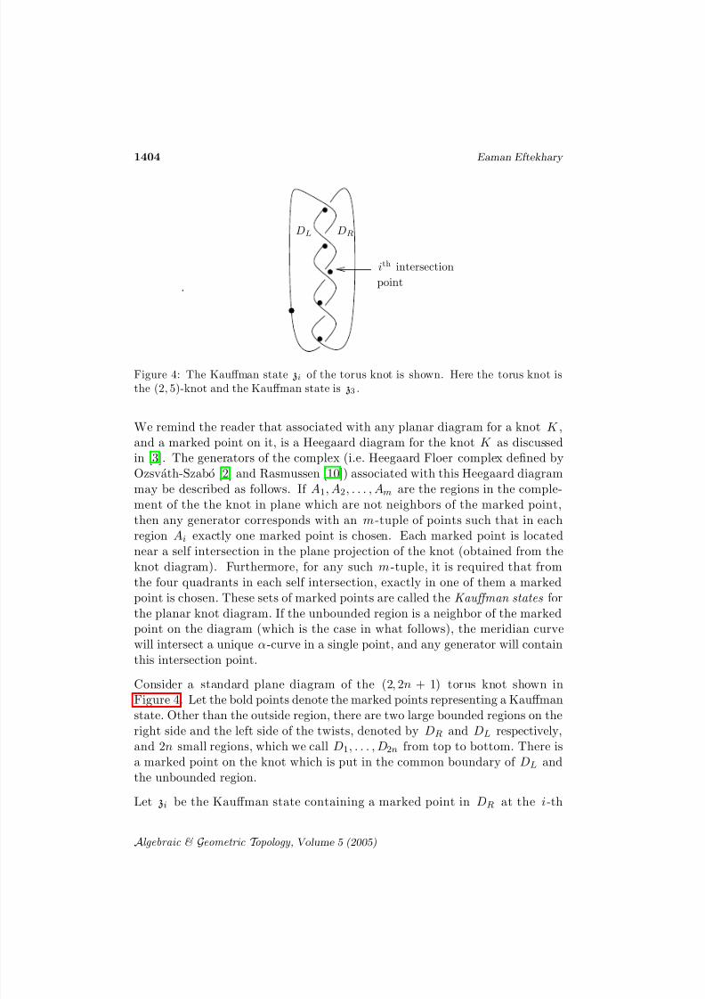
Figure 4: The Kauffman state zi of the torus knot is shown. Here the torus knot isthe (2, 5)-knot and the Kauffman state is z3 .

We remind the reader that associated with any planar diagram for a knot K ,and a marked point on it, is a Heegaard diagram for the knot K as discussedin [3]. The generators of the complex (i.e. Heegaard Floer complex defined byOzsvath-Szabo [2] and Rasmussen [10]) associated with this Heegaard diagrammay be described as follows. If A1, A2, . . . , Am are the regions in the comple-ment of the the knot in plane which are not neighbors of the marked point,

then any generator corresponds with an m-tuple of points such that in eachregion Ai exactly one marked point is chosen. Each marked point is locatednear a self intersection in the plane projection of the knot (obtained from theknot diagram). Furthermore, for any such m-tuple, it is required that fromthe four quadrants in each self intersection, exactly in one of them a markedpoint is chosen. These sets of marked points are called the Kauffman states forthe planar knot diagram. If the unbounded region is a neighbor of the markedpoint on the diagram (which is the case in what follows), the meridian curvewill intersect a unique α-curve in a single point, and any generator will containthis intersection point.

Consider a standard plane diagram of the (2, 2n + 1) torus knot shown in

Figure 4. Let the bold points denote the marked points representing a Kauffmanstate. Other than the outside region, there are two large bounded regions on theright side and the left side of the twists, denoted by DR and DL respectively,and 2n small regions, which we call D1, . . . , D2n from top to bottom. There isa marked point on the knot which is put in the common boundary of DL andthe unbounded region.

Let zi be the Kauffman state containing a marked point in DR at the i-th





add twists tomake a zeroframed

longitudewinding

l α1

x1

y1

x2

y2

Figure 5: The Heegaard diagram associated with the trefoil is presented. On thehandle appearing on the right-hand-side we may do enough twists so that the diagram

represents a three-manifold with b1 = 1 . The winding is done on the left-hand-sidehandle. The bold curves are the α curves and the rest of them are the β curves.

intersection. There is a unique Kauffman state described by this property.Moreover, the states z1, . . . , z2n+1 will be all of the Kauffman states of (gen-erators of the Heegaard Floer complex for) the (2, 2n + 1) torus knot. As itwas noted earlier the Kauffman states are in one-to-one correspondence withthe generators. So each zi may be thought of as a set of 2n + 1 intersectionpoints in the Heegaard diagram which, together with the unique intersectionpoint on the meridian, give a generator for the Heegaard Floer complex. Thesetwo alternative ways of thinking about the Kauffman states zi are used in the

following.

The Spinc grading of the Kauffman states is described via s( zi) = i − n − 1,and the (relative) Maslov grading by µ( zi) = i − 1, all in the sense of [2]. Notethat s( zi) ∈ Z = Spinc(S 30(K )) is the well-defined Spinc structure used in theHeegaard Floer homology of Ozsvath-Szabo ([2]) and Rasmussen ([10]).

After winding l along m sufficiently many times, the proof of theorem 3.2 (cf.





section 5 of [4]) may be copied to prove the following:

Lemma 4.1 For any Spinc class

s ∈ 12 + Z = 1

2PD[µ] + Spinc(S 30(K )),

with the property |s| < n = genus (T (2, 2n +1)), all the generators in the class s are of the form:

xij = {xi} ∪ z j, yij = {yi} ∪ z j,

where z j s are considered as sets of 2n + 1 intersection points in the Heegaarddiagram, and x1, x2, . . . , y1, y2, . . . are the intersection points on l which resultfrom winding it around the meridian µ.

These generators will be called Kauffman states for longitude Floer homology or just Kauffman states if it is clear from the context that longitude Floer complexis considered.

It is easy to check that the following assignments, satisfy all the relative Maslovgrading computations and the equations for Spinc differences:

−µ(yij) = µ(xij) = j − n − 32 ,

s(xij) = s(yij) = j − i − n − 12 .

(7)

Here we are assigning rational values as the Maslov grading, which is an abuseof notation. However, note that here we are only interested in relative grading,and the relative Maslov gradings are still by integers.

The Kauffman states which lie in the Spinc structure s = s − 12 ∈ 1

2 + Z arethose xij and yij for which j − i = n + s.

Remember that there cannot b e any boundary map going from xij to yij .Furthermore, if there exists a map from xij to xi+k,j−k regardless of what N is,then there is a map from xl,j to xl+k,j−k regardless of what N is, for all otherl . Conversely, if there is no map from xij to xi+k,j−k regardless of what N is,then there is no map from xl,j to xl+k,j−k . This is because of the isomorphismbetween the domains of the disks between the corresponding generators.

Since we already know that CFL(K ) is symmetric with respect to the Spinc

structures ∈ 1

2 + Z ≃ 12PD[µ] + Spinc(S 30(K )),

and since the genus of K = T (2, 2n+1) is n, it is enough to compute CFL(K, s)for the Spinc structures 0 < s < n . Here µ represents the meridian of the knotK .





If 0 < s < n, then because of the above Maslov grading of the generators, therecannot be any boundary maps from any of yij ’s to any of xkl ’s in Spinc class s.Thus, the only boundary maps that should be studied are the boundary mapswithin xij ’s, as well as the boundary maps within ykl ’s.

(a) (b)

Figure 6: The domain between xij and x(i−1)(j−1) (b) is a modification of the domainconnecting the two generators zj and zj−1 (a) in the Heegaard diagram obtained fromthe alternating projection of K . If there are k small circles in the domain on the left,we will denote it by Dk . Note that the bold curves are in α while the regular curvesare in β .

If xkl appears in the boundary of xij , then they are in the same Spinc class andthe Maslov grading of the first generator is one less than the Maslov grading of the second generator. This implies that k = i − 1 and j = l − 1. The domainbetween xij and x(i−1)( j−1) is a modification of the domain connecting the twogenerators z j and z j−1 in the Heegaard diagram obtained from the alternatingprojection of K shown in Figure 4. If j = 2l + 1 for some l , then the domainbetween z j and z j−1 is illustrated in Figure 6(a), while the modified domainconnecting xij and x(i−1)( j−1) will be of the type shown in Figure 6(b). Letus denote this last domain by Dk , where k is the number of circles inside therectangle.

The moduli spaces M(Dk) and M(Dk−1) are in fact cobordant, since Dk isobtained from Dk−1 via the operation of adding a handle. This can be provedusing the usual argument of Ozsvath and Szabo for the invariance of the Floerhomology when we add a one handle to the surface, and a pair of cancellingcurves to α and β (see [4]).

To show that the total contribution of the domain Dk to the boundary map is±1, we only have to show this for D = D0 .





Lemma 4.2 Let D be as above. Then the algebraic sum of the points in the moduli space

M(D) =M(D)

R

is ±1.

Proof Consider the embedding of the domain D in a genus three Heegaarddiagram which is shown in Figure 7. Let the bold and the regular curves denotethe α and the β curves respectively. Choose αi ’s and β j ’s so that the α curve

which spins around the center is α1 and the β curve cutting it several times isβ 1 .

Consider the small dotted circle θ1 in Figure 7 and complete it into a set of three disjoint linearly independent simple closed curves by adding Hamiltonianisotopes of the curves β 2 and β 3 , which we will call θ2 and θ3 respectively. Wechoose them so that θi intersects β i in a pair of transverse cancelling intersectionpoints, for i = 2, 3. Call the resulting sets of curves α, β and θ .

The triple Heegaard diagram

H =

Σ3, α, θ , β ; u,v,w

,

with u, v and w being the marked points of Figure 7, induces a chain map

F : CF (α, θ) ⊗ CF (θ , β) −→ CF (α, β).

The map F is defined through a count of holomorphic triangles which missthe marked points u, v and w (see [4, 5] for more details on the construction

of F ). The complex CF (θ , β) gives the Floer homology associated with thethree-manifold (S 1 × S 2)#(S 1 × S 2). There is a top generator of this homology

group which we may denote by Θ . The complex CF (α, θ) has precisely twogenerators x and y , with a single boundary map going from x to y. The imageF (x × Θ) will have several terms, probably in different Spinc classes.

Denote the intersection p oints of α1

and β 1

in the spiral by x1

, x2

, . . . , sothat x1 is the one that is closest to the center of the spiral. Each xi may becompleted to a generator of CF (α, β) precisely in two ways, which will bedenoted by {xi} ∪ z and {xi} ∪ w. We may choose them so that {x1} ∪ z

and {x2} ∪ w are in the same Spinc class. Under this assumption the domainconnecting them is the domain D introduced above. Denote this same Spinc

class by s, and denote the part of the image of F in the Spinc class s by F s .Clearly F s is also a chain map.





u v w

θ1

α1

α2

α3

β 1

β 2

β 3

Figure 7: The domain D may be embedded in a genus three Heegaard diagram. Thecurve winding around the center is α1 , which is completed to α = {α1, α2, α3}. Thecurve β 1 ∈ β = {β 1, β 2, β 3} cuts α1 several times. The dotted small circle is θ1 whichis completed to a triple θ by adding the Hamiltonian isotopes θ2 and θ3 of β 2 andβ 3 . The intersection points between β 1 and α1 are labelled x1, x2, . . . with x1 theintersection point on the right hand side of θ1 in the picture.

It is not hard to check, using the energy filtration of [5], that we would have

F s(x ⊗ Θ) = ±{x1} ∪ z + lower energy terms, and

F s(y ⊗ Θ) = ±{x2} ∪ w + lower energy terms.

It is then an algebraic fact that {x2} ∪ w appears in the boundary of {x1} ∪ z

with coefficient ±1, which is on its own a result of ∂ (x ⊗ Θ) = y ⊗ Θ. Thiscompletes the proof of the lemma.

This lemma implies that ∂ (x(i)(2l+1)) = ±x(i−1)(2l) . Since ∂ ◦ ∂ = 0, we mayconclude that ∂ (x(i)(2l)) = 0 for all i, l , unless i is too large (i.e. irrelevant).Similarly we may deduce that

∂ (y(i)(2l)) = y(i−1)(2l−1), and

∂ (y(i)(2l+1)) = 0.

We may summarize all these information as the following theorem.

Theorem 4.3 Let K = T (2, 2n + 1) denotes the (2, 2n + 1) torus knot in S 3 .Then for any Spinc structure

s ∈ 12 + Z ≃ 1

2PD[µ] + Spinc(S 30(K )),





the longitude Floer homology of K is trivial if |s| > n. Otherwise it is givenby

HFL(K, s) = Z(−n+ 1

2) ⊕ Z(ǫ(s)s),

where ǫ(s) = (−1)n−1

2−s , and Z(k) denotes a copy of Z in (relative) Maslov

grading k .

Proof The proof for s > 0 is just an algebraic result of the cancellationsinduced by the map ∂ above. For s < 0, it is the result of the symmetry on HFL(K ).

5 A Heegaard diagram for Whitehead double

In this section, we will construct an appropriate Heegaard diagram for K L outof a Heegaard diagram for K .

Suppose that (Σ; δ ; {m = γ 1}∪ γ 0) is a Heegaard diagram for K together withan extra curve l (As usual, δ = {δ1, . . . , δg} and γ 0 = {γ 2, . . . , γ g}). Here lis the curve with the property that it intersects the meridian m = γ 1 exactlyonce but does not cut any other γ curve. The curve l represents the longitude

of the knot K in such a way that

(Σ; δ ; {l} ∪ γ 0)

is a Heegaard diagram for S 30(K ). Define

γ = {l} ∪ γ 0.

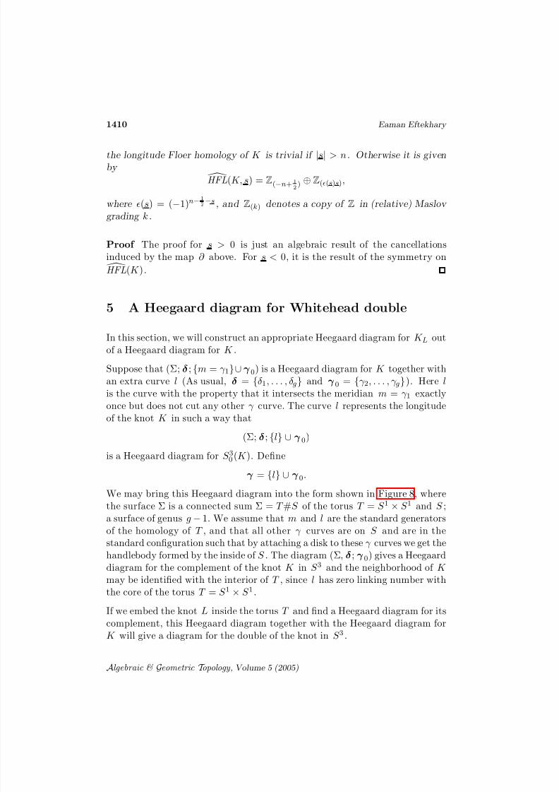
We may bring this Heegaard diagram into the form shown in Figure 8, wherethe surface Σ is a connected sum Σ = T #S of the torus T = S 1 × S 1 and S ;a surface of genus g − 1. We assume that m and l are the standard generatorsof the homology of T , and that all other γ curves are on S and are in thestandard configuration such that by attaching a disk to these γ curves we get the

handlebody formed by the inside of S . The diagram (Σ, δ ; γ 0) gives a Heegaarddiagram for the complement of the knot K in S 3 and the neighborhood of K may be identified with the interior of T , since l has zero linking number withthe core of the torus T = S 1 × S 1 .

If we embed the knot L inside the torus T and find a Heegaard diagram for itscomplement, this Heegaard diagram together with the Heegaard diagram forK will give a diagram for the double of the knot in S 3 .





(a)

(b)

m

l

δ1

n

γ z

w

λ

α1

α2

α3α4

β 1 β 2

β 3β 4

Figure 8: (a) A Heegaard diagram associated with K . Here m denotes the meridian,and l is the longitude of the knot. The curve δ1 is the unique δ curve cutting m. (b)A Heegaard diagram for L in the solid torus. The thicker curves denote the α curves,and the thinner ones are β ’s. The curve n denotes the meridian of L .





More precisely, consider the Heegaard diagram shown in Figure 8 (b) for theunknot sitting inside the solid torus. Here the thick curves denote the α circles,while the thin ones are β ’s. There is an extra curve λ shown in the picture,which we save for the later purposes. There is a special α-curve denoted byγ in the figure, which represents the generator of the first homology groupH 1(D2 × S 1, Z) of the solid torus.

If we attach a disk to each α curve, except for γ , in this Heegaard diagramand a disk to each of the β circles other than the meridian n, we will get thecomplement of the knot L inside a solid torus S 1 × D2 .

Put this solid torus inside the torus T . Attach the surface of the solid torusand T by a one-handle connecting the intersection of γ 1 and l on T to theintersection of γ and λ on the Heegaard diagram for L.

The result of this operation may be regarded as a connected sum of the surfacesΣ and C . Here (Σ, δ , {m} ∪ γ 0) is the above Heegaard diagram for K , and C is the surface in the Heegaard diagram of L used above.

Denote by (n, β 1, . . . , β 4) the β curves on C and by (γ, α1, . . . , α4) the α curves,as is shown in Figure 8 (b).

In order to find a Heegaard diagram for the complement of the Whitehead

double in the sphere S

3

, we have to fill the space between the solid torus andthe torus T . Looking at T #C , there are two disks which sit in the empty spacebetween T and the solid torus. Namely, if we cut the union by a horizontalplane, the intersection will look like the left hand side of Figure 9. There is adisk bounded by the connected sum γ #l . This disk is dashed in Figure 9.

We may also cut the torus with a vertical plane. If the cut is made in a waythat it passes through m and λ, and cuts the handle connecting the solid torusand the torus T , then the cut will look like what is shown on the right handside of Figure 9. Again, there is a disk which is dashed in the picture, with aboundary which is the connected sum λ#m = λ#γ 1 .

The result of this operation is a Heegaard diagram for the Whitehead doubleof K :

(Σ#C ; {n, β 1, . . . , β 4} ∪ δ ; {α1, . . . , α4} ∪ {λ#m, γ #l} ∪ γ 0; z, w),

where z and w are two base points which are put on the two sides of thecurve n on C . We will use this Heegaard diagram to relate the Ozsv ath-SzaboFloer homology of the Whitehead double of K to the longitude Floer homologydiscussed in the earlier sections.





m

m

l

l

α

λγ

γ

cut along the planepassing though l, α cut along the curve m

Figure 9: If we cut the torus T by a horizontal plane, the intersection will be as shownon the left side. There is a disk which is dashed in this picture with boundary γ #l . If the cut is vertical and on the connecting handle, the picture is as shown on the right.Again, there is a disk with boundary λ#m

.

6 Whitehead double; homology computation

In order to obtain the Ozsvath-Szabo Floer homology groups we should firstform the chain complex by identifying the relevant generators of this Heegaarddiagram.

There are two types of generators for this Heegaard diagram:

(1) The Kauffman states which are in correspondence with a pair of generatorsof the form {x, y}, where x is a generator of

(C ; γ, α1, . . . , α4; n, β 1, . . . , β 4),

and y is a generator of (Σ, δ ; {m} ∪ γ 0). We call these generators meridian

Kauffman states.

(2) The Kauffman states which are associated with a pair of generators of theform {x, y}, where x is a generator of

(C ; λ, α1, . . . , α4; n, β 1, . . . , β 4),





and y is a generator of (Σ, δ ; {l} ∪ γ 0). We call these generators the longitude

Kauffman states.

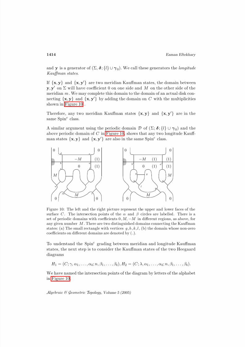
If {x, y} and {x, y′} are two meridian Kauffman states, the domain betweeny, y′ on Σ will have coefficient 0 on one side and M on the other side of themeridian m. We may complete this domain to the domain of an actual disk con-necting {x, y} and {x, y′} by adding the domain on C with the multiplicitiesshown in Figure 10 .

Therefore, any two meridian Kauffman states {x, y} and {x, y′} are in thesame Spinc class.

A similar argument using the periodic domain D of (Σ; δ ; {l} ∪ γ 0) and theabove periodic domain of C in Figure 10, shows that any two longitude Kauff-man states {x, y} and {x, y′} are also in the same Spinc class.

−M −M

M

M M

M

(1)

(1)

(1)

(1)(1)

(1)

0

00

00

0

00

00

ab

c

d e

f

gh

k

l

m

np

q

r

a′b′

Figure 10: The left and the right picture represent the upper and lower faces of thesurface C . The intersection points of the α and β circles are labelled. There is aset of periodic domains with coefficients 0, M, −M in different regions, as above, forany given number M . There are two distinguished domains connecting the Kauffmanstates: (a) The small rectangle with vertices g, h, k, l, (b) the domain whose non-zerocoefficients on different domains are denoted by (.).

To understand the Spinc grading between meridian and longitude Kauffmanstates, the next step is to consider the Kauffman states of the two Heegaarddiagrams

H 1 = (C ; γ, α1, . . . , α4; n, β 1, . . . , β 4), H 2 = (C ; λ, α1, . . . , α4; n, β 1, . . . , β 4).

We have named the intersection points of the diagram by letters of the alphabetin Figure 10.





The Kauffman states of H 1 will be the following list

x1 = {n,d,h,p,f },

x2 = {n,c,g,r,f },

x3 = {n,g,c,q,e}.

It is easy to see that x1 and x2 are in the same Spinc class and there is adisk between them, which is disjoint from the shaded area, where the handle isattached to the surface C . This disk supports a unique holomorphic represen-tative. The numbers in parenthesis denote the nonzero coefficients of the disk

between these two Kauffman states.The Kauffman state x3 is in a higher Spinc class. This means that s(x1) + 1 = s(x2) + 1 = s(x3).

The relative Maslov grading of any two Kauffman states (of the meridian orlongitude type) {x, y} and {x, y′} is the same as the relative Maslov index of the states y and y′ . So the contribution of all the Kauffman states of the form{x, y}, for a fixed x, is equal (up to a sign) to the Euler characteristic of HF (S 3)

or the Euler characteristic of HF (S 30(K )), depending on whether {x, y}’s aremeridian Kauffman states or longitude Kauffman states, respectively. Thisimplies that the total contribution of longitude Kauffman states to the Euler

characteristic in different Spinc

structures is zero. For each of xi we will geta contribution equal to ±1. The contribution from x1 is cancelled against thecontribution from x2 , so the only Spinc structure for which the contributionis nonzero, is s(x3). The conclusion is that s({x3, •}) = s(x3) = 0, since the

Euler characteristic of HFK (K L) gives the symmetrized Alexander polynomialof K L (which is trivial). Moreover, as a result of the previous discussion, wehave:

s({x, y}) = s(x), for all meridian Kauffman states {x, y}.

Here the right hand side is a Spinc class associated with the Heegaard diagramH 1 . So s(x1) + 1 = s(x2) + 1 = s(x3) = 0, and there is no meridian Kauffmanstate in the Spinc class s = 1.

Now we turn to the Kauffman states of H 2 . We will show that some of themnaturally cancel against each other. Then we will identify the remaining ones,and will compute the Spinc -grading of the corresponding longitude Kauffmanstates.

There is a small rectangle bounded by the intersection points h,g,l,k on thelower face of the surface. For any pair of Kauffman states for the Whitehead





double which are of the form {g,k, •} and {h,l, •}, the domain of the diskbetween these two states is this rectangle, which supports a unique holomorphicrepresentative. There are six of these pairs. We may cancel them againsteach other, in the expense that having two Kauffman states with a disk of thefollowing type connecting them, we will not be able to argue that there is noboundary map between the two Kauffman states. The disks considered aboveare the ones with negative coefficients in the rectangle. Since we will not facethis situation in what follows, we simply choose to cancel them against eachother. For a more careful explanation of this method we refer the reader toRasmussen’s paper [9].

Here is a list of the remaining Kauffman states:

z1 = {a,q,g,m,c},

z2 = {a′,q ,g ,m,c},

z3 = {b,h,m,p,f },

z4 = {b′,h,m,p,f }.

One may check by considering the domains that

s(z1) = s(z2) + 1 = s(z3) + 1 = s(z4) + 2. (8)

In order to see what the absolute grading of these states is, move δ1 ( the unique

δ curve that intersects m) by an isotopy to create a pair of intersection pointswith l . One of them has the property that together with the intersection of l and m and the intersection of m and δ1 , they form the vertices of a smalltriangle. Call this point x0 and let y0 be the intersection point of m and δ1 .If y = {y0, •} is a Kauffman state for (Σ; δ ; {m} ∪ γ 0), then {x0, •} will be aKauffman state for

(Σ; δ ; {l} ∪ γ 0).

There is a domain representing a disk with zero coefficients on z and w whichconnects the two Kauffman states z3 ∪ {y0, •} and x3 ∪ {x0, •}. So for anylongitude Kauffman state of the form zi ∪ {•} we may compute the Spinc

grading via the formula:

s(z1 ∪ {•}) − 1 = s(z2 ∪ {•}) = s(z3 ∪ {•}) = s(z4 ∪ {•}) + 1 = 0. (9)

So the only Kauffman states in the Spinc structure s = 1 that remain, are thoseof the form z1 ∪ y , where y is some Kauffman state on the Heegaard diagramH 2 (which is a potential Heegaard diagram for the longitude Floer homology).

Suppose that z1 ∪ y and z1 ∪ y′ are two Kauffman states in our Heegaarddiagram. Since the states do not differ on C , the only possibility for a domain





between the two states is that the coefficients in all of the regions on C arezero except for the regions where a coefficient equal to ±M is assigned asin Figure 10. In any such domain, there are regions with both M and −M as coefficients. Furthermore, these domains do not use the small rectangleconsidered before. So the only case where there is potentially a boundary mapfrom z1 ∪ y to z1 ∪ y′ is when we have M = 0.

In this case the four regions around the connecting handle will get coefficientsequal to zero. This means that the disk is completely supported on Σ. Fur-thermore if we put two marked points z′ and w′ on the two sides of l at the

intersection of l with β 1 , the above discussion shows that the domains of thedisks between these points will have zero coefficients in the regions associatedwith z′ and w′ .

So, the disks that contribute to the boundary operator are in 1-1 correspondencewith the disks between y and y′ in the hat theory assigned to the Heegaarddiagram

(Σ, δ ; {l} ∪ γ 0; z′, w′).

The above discussion shows that the generators and all the boundary maps inthe Ozsvath-Szabo Floer homology of K L in Spinc structure s = 1 are exactlythe same as those appearing in

CFL(K ) = i∈Z+ 1

2

CFL(K, i).

The Spinc grading of CFL(K ), and that of the homology groups HFL(K ) areforgotten when we compute the Ozsvath-Szabo Floer homology of the White-head double, and the isomorphism is an isomorphism of groups (relatively)graded by the Maslov index.

We have proved the following theorem:

Theorem 6.1 Let K L denote the Whitehead double of a knot K in S 3 . The Ozsvath-Szabo Floer homology groups HFK (K L, ±1) are isomorphic to the

group HFL(K ) = i∈Z+ 1

2 HFL(K, i) as (relatively) Z-graded abelian groups

with the (relative) grading on both sides coming from the Maslov grading.

As a corollary of this theorem and the results of the previous section we have:

Corollary 6.2 Let K = T (2, 2n + 1) denote the (2, 2n + 1) torus knot and letK L be the Whitehead double of K . Then the Ozsvath-Szabo Floer homology





groups HFK (K L, +1) in different (relative) Maslov gradings are described as follows:

µ : n n − 2 . . . −n + 2 −n + 1 HFK : Z ⊕ Z Z ⊕ Z . . . Z ⊕ Z

2ni=1 Z

Remark 6.3 The longitude Floer homology may be defined for a knot ina three-manifold Y , and as such, it enjoys very nice surgery formulas. Wepostpone a discussion of these subjects to a future paper.

References

[1] G Burde, H Zieschang, Knots, de Gruyter Studies in Mathematics 5, Walterde Gruyter & Co. Berlin (2003) MR1959408

[2] P Ozsvath, Z Szabo, Holomorphic disks and knot invariants, to appear inAdvances in Math, arXiv:math.GT/0209056

[3] P Ozsvath, Z Szabo, Heegaard Floer homology and alternating knots,Geom. Topol. 7 (2003) 225–254 MR1988285

[4] P Ozsvath, Z Szabo, Holomorphic disks and topological invariants for closed

three-manifolds, to appear in Annals of Math. arXiv:math.SG/0101206

[5] P Ozsvath, Z Szabo, Holomorphic disks and three-manifold invariants: prop-

erties and applications, to appear in Annals of Math. arXiv:math.SG/0105202[6] P Ozsvath, Z Szabo, Heegaard Floer homologies and contact structures,

arXiv:math.SG/0210127

[7] P Ozsvath, Z Szabo, Knot Floer homology and the four-ball genus,Geom. Topol. 7 (2003) 615–639 MR2026543

[8] P Ozsvath, Z Szabo, Holomorphic disks and genus bounds,Geom. Topol. 8 (2004) 311–334 MR2023281

[9] J A Rasmussen, Floer homology of surgeries on two-bridge knots,Algebr. Geom. Topol. 2 (2002) 757–789 MR1928176

[10] textbfJ A Rasmussen, Floer homology and knot complements, PhD thesis, Har-vard Univ. arXiv:math.GT/0306378

[11] L Rudolph, The slice genus and the Thurston-Bennequin invariant of a knot ,Proc. Amer. Math. Soc. 125 (1997) 3049–3050 MR1443854

Mathematics Department, Harvard University 1 Oxford Street, Cambridge, MA 02138, USA

Email: [email protected]

Received: 15 July 2004

http://www.ams.org/mathscinet-getitem?mr=1959408

http://arxiv.org/abs/math.GT/0209056

http://www.maths.warwick.ac.uk/gt/GTVol7/paper6.abs.html


http://arxiv.org/abs/math.SG/0101206







http://www.maths.warwick.ac.uk/agt/AGTVol2/agt-2-32.abs.html




mailto:[email protected]

mailto:[email protected]




http://www.maths.warwick.ac.uk/agt/AGTVol2/agt-2-32.abs.html












eaman eftekhary- longitude floer homology and the whitehead double

Documents